Embed Size (px)
Citation preview

ME338A - Final project - Paper review - due in class Thu, March 11, 2010, 11am
Constitutive modelling of passive myocardiumA structurally-based framework for material characterization
Gerhard A. Holzapfel & Ray W. OgdenPhilosophical Transactions of the Royal Society A 2009,367:3445-3475.
This final project will demonstrate that during the past 10 weeks, you have learned toread state of the art continuum mechanics literature. Gerhard Holzapfel and Ray Ogden,two leading scientists in continuum biomechanics, have recently published a manuscriptthat introduces a new continuum mechanics model for passive cardiac muscle tissue.
1 Read the publication and try to understand what it is all about. You do not neces-sarily need to understand all the equations. You can briefly glance over section 6, itis not relevant for this final project.
2 Summarize the manuscript in less than 200 words.
3 Ogden & Holzapfel use a slightly different notation than we have used in class, i.e.,they do not use dots to indicate scalar products. Rewrite equations (3.1) to (3.14) inour tensor notation, i.e., use the dot for scalar products when appropriate.
4 Rewrite equations (3.1) to (3.14) in index notation. For each equation, state in brack-ets whether it is a scalar, vectorial, or second order tensorial equation.
5 In section 4, Ogden & Holzapfel review existing constitutive models for passivecardiac tissue. They discuss three transversely isotropic models (4.1), (4.2), and (4.3)and three orthotropic models (4.5), (4.7), and (4.8). Summarize these six models in atable. For each model, list the first author, the year it was published, the invariantsit is based on, and the parameters that are needed.
6 Figure 4 illustrates the deformation state of simple shear. Calculate the Green La-grange strain tensor E = 1
2 [ F t · F − I ] from the deformation gradient given in (5.9)and sketch the deformed configuration in the f s-plane.
7 Equation (5.38) is the key equation of the paper. It introduces the free energy func-tion for myocardial tissue. Describe its three terms and explain the required materialparameters.
8 Most soft biological tissues are incompressible and anisotropic. How are incom-pressibility and anisotropy handled in this constitutive formulation?
9 Review the publication with the help of the attached spreadsheet. Use commonsense to answer the questions you cannot answer based on your current continuummechanics knowledge. There are no wrong answers, and we will not take off pointsas long as you can justify your opinion.
1

ME338A Continuum Mechanics Review Form
InstructionsPlease rate this manuscript on a scale of 1-5, with 1 indicating greatest degree or best,and 5 indicating least degree or poor. You must also provide comments to the authors inprose. It is not acceptable to merely fill out numbers, and return the review.
Manuscript title
Authors
Summary (required brief summary of the context)
Presentation ( best ) 1 2 3 4 5 (poor)is clearly written � � � � �title is appropriate � � � � �abstract is appropriate � � � � �figures and tables are adequate � � � � �problem statement is clear � � � � �provides appropriate detail � � � � �describes limitations � � � � �references are adequate � � � � �
Comments (required in addition to the number ratings above)
Significance ( best ) 1 2 3 4 5 (poor)represents important advance � � � � �addresses importand and realistic problem � � � � �is likely to scale up to realistic problems � � � � �provides new evidence for existing technique � � � � �
1

ME338A Continuum Mechanics Review Form
Comments (required in addition to the number ratings above)
Originality ( best ) 1 2 3 4 5 (poor)novel approach or combination of approaches � � � � �has not been published before � � � � �points out differences from related research � � � � �reformulates a problem in an important way � � � � �
Comments (required in addition to the number ratings above)
Technical content ( best ) 1 2 3 4 5 (poor)evaluates effectiveness of techniques � � � � �is supported with sound arguments � � � � �is supported with theoretical analysis � � � � �is supported with experimental results � � � � �is technically sound � � � � �
Additional comments to the autors
Overall recommendation � accept � marginal � reject
Your confidence in recommendation � strong � medium � weak
Confidential commments to the editor
Confidential reviewer name
2
doi: 10.1098/rsta.2009.0091, 3445-3475367 2009 Phil. Trans. R. Soc. A
Gerhard A. Holzapfel and Ray W. Ogden characterizationstructurally based framework for material Constitutive modelling of passive myocardium: a
Referencesl.html#ref-list-1http://rsta.royalsocietypublishing.org/content/367/1902/3445.ful
This article cites 35 articles, 10 of which can be accessed free
Rapid response1902/3445http://rsta.royalsocietypublishing.org/letters/submit/roypta;367/
Respond to this article
Subject collections
(118 articles)biomedical engineering � collectionsArticles on similar topics can be found in the following
Email alerting service herein the box at the top right-hand corner of the article or click Receive free email alerts when new articles cite this article - sign up
http://rsta.royalsocietypublishing.org/subscriptions go to: Phil. Trans. R. Soc. ATo subscribe to
This journal is © 2009 The Royal Society
on February 17, 2010rsta.royalsocietypublishing.orgDownloaded from
Phil. Trans. R. Soc. A (2009) 367, 3445–3475doi:10.1098/rsta.2009.0091
Constitutive modelling of passive myocardium:a structurally based framework for material
characterizationBY GERHARD A. HOLZAPFEL1,2,* AND RAY W. OGDEN3
1Department of Solid Mechanics, School of Engineering Sciences, RoyalInstitute of Technology (KTH ), Osquars Backe 1, 100 44 Stockholm, Sweden
2Institute of Biomechanics, Center of Biomedical Engineering, Graz Universityof Technology, Kronesgasse 5-I, 8010 Graz, Austria
3Department of Mathematics, University of Glasgow, University Gardens,Glasgow G12 8QW, UK
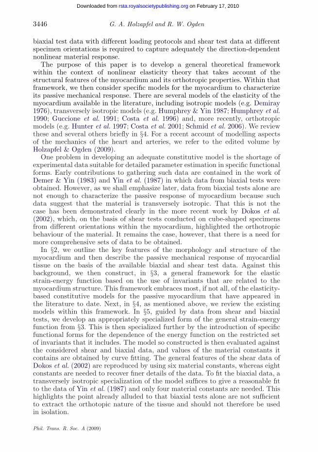
In this paper, we first of all review the morphology and structure of the myocardiumand discuss the main features of the mechanical response of passive myocardium tissue,which is an orthotropic material. Locally within the architecture of the myocardiumthree mutually orthogonal directions can be identified, forming planes with distinctmaterial responses. We treat the left ventricular myocardium as a non-homogeneous,thick-walled, nonlinearly elastic and incompressible material and develop a generaltheoretical framework based on invariants associated with the three directions. Withinthis framework we review existing constitutive models and then develop a structurallybased model that accounts for the muscle fibre direction and the myocyte sheet structure.The model is applied to simple shear and biaxial deformations and a specific form fittedto the existing (and somewhat limited) experimental data, emphasizing the orthotropyand the limitations of biaxial tests. The need for additional data is highlighted. A briefdiscussion of issues of convexity of the model and related matters concludes the paper.
Keywords: myocardium; constitutive modelling; orthotropy; muscle fibres;myocyte sheet structure
1. Introduction
Of central importance for the better understanding of the fundamentalmechanisms underlying ventricular mechanics are: (i) realistic descriptions ofthe three-dimensional geometry and structure of the myocardium, (ii) continuumbalance laws and boundary conditions and, most importantly, (iii) constitutiveequations that characterize the material properties of the myocardium, includingtheir spatial and temporal variations, together with statistical parameterestimation and optimization, and validation. To characterize the materialproperties, it is essential to have available comprehensive force–deformation datafrom a range of different deformation modes. In particular, a combination of*Author for correspondence ([email protected]).
One contribution of 12 to a Theme Issue ‘Mechanics in biology: cells and tissues’.
This journal is © 2009 The Royal Society3445
on February 17, 2010rsta.royalsocietypublishing.orgDownloaded from
3446 G. A. Holzapfel and R. W. Ogden
biaxial test data with different loading protocols and shear test data at differentspecimen orientations is required to capture adequately the direction-dependentnonlinear material response.
The purpose of this paper is to develop a general theoretical frameworkwithin the context of nonlinear elasticity theory that takes account of thestructural features of the myocardium and its orthotropic properties. Within thatframework, we then consider specific models for the myocardium to characterizeits passive mechanical response. There are several models of the elasticity of themyocardium available in the literature, including isotropic models (e.g. Demiray1976), transversely isotropic models (e.g. Humphrey & Yin 1987; Humphrey et al.1990; Guccione et al. 1991; Costa et al. 1996) and, more recently, orthotropicmodels (e.g. Hunter et al. 1997; Costa et al. 2001; Schmid et al. 2006). We reviewthese and several others briefly in §4. For a recent account of modelling aspectsof the mechanics of the heart and arteries, we refer to the edited volume byHolzapfel & Ogden (2009).
One problem in developing an adequate constitutive model is the shortage ofexperimental data suitable for detailed parameter estimation in specific functionalforms. Early contributions to gathering such data are contained in the work ofDemer & Yin (1983) and Yin et al. (1987) in which data from biaxial tests wereobtained. However, as we shall emphasize later, data from biaxial tests alone arenot enough to characterize the passive response of myocardium because suchdata suggest that the material is transversely isotropic. That this is not thecase has been demonstrated clearly in the more recent work by Dokos et al.(2002), which, on the basis of shear tests conducted on cube-shaped specimensfrom different orientations within the myocardium, highlighted the orthotropicbehaviour of the material. It remains the case, however, that there is a need formore comprehensive sets of data to be obtained.
In §2, we outline the key features of the morphology and structure of themyocardium and then describe the passive mechanical response of myocardialtissue on the basis of the available biaxial and shear test data. Against thisbackground, we then construct, in §3, a general framework for the elasticstrain-energy function based on the use of invariants that are related to themyocardium structure. This framework embraces most, if not all, of the elasticity-based constitutive models for the passive myocardium that have appeared inthe literature to date. Next, in §4, as mentioned above, we review the existingmodels within this framework. In §5, guided by data from shear and biaxialtests, we develop an appropriately specialized form of the general strain-energyfunction from §3. This is then specialized further by the introduction of specificfunctional forms for the dependence of the energy function on the restricted setof invariants that it includes. The model so constructed is then evaluated againstthe considered shear and biaxial data, and values of the material constants itcontains are obtained by curve fitting. The general features of the shear data ofDokos et al. (2002) are reproduced by using six material constants, whereas eightconstants are needed to recover finer details of the data. To fit the biaxial data, atransversely isotropic specialization of the model suffices to give a reasonable fitto the data of Yin et al. (1987) and only four material constants are needed. Thishighlights the point already alluded to that biaxial tests alone are not sufficientto extract the orthotopic nature of the tissue and should not therefore be usedin isolation.
Phil. Trans. R. Soc. A (2009)
on February 17, 2010rsta.royalsocietypublishing.orgDownloaded from

Modelling of passive myocardium 3447
In §6, we examine the form of strain-energy function constructed withreference to inequalities that ensure ‘physically reasonable response’, includingthe monotonicity of the stress deformation behaviour in uniaxial tests and notionsof convexity and strong ellipticity in three dimensions. These all require, inparticular, that the material constants included in various terms contributingto the strain energy are positive, which is consistent with the values obtained infitting the data. Finally, §7 is devoted to a concluding discussion.
2. Morphology, structure and typical mechanical behaviourof the passive myocardium
(a) Morphology and structure
The human heart consists of four chambers, namely the right and left atria, whichreceive blood from the body, and the left and right ventricles, which pump bloodaround the body. For a detailed description of the individual functionalities ofthese four chambers, see Katz (1977). There is still an ongoing debate concerningthe structure of the heart (Gilbert et al. 2007), and, in particular, the anisotropiccardiac microstructure. One approach describes the heart as a single musclecoiled in a helical pattern, whereas the other approach considers the heart tobe a continuum composed of laminar sheets, an approach we are adopting in thepresent work.
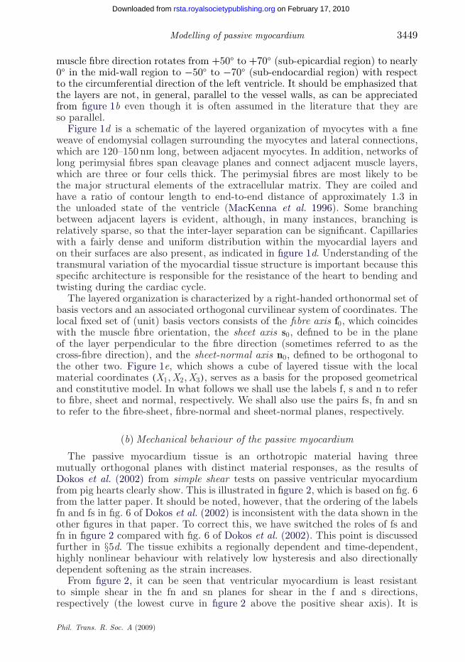
The left ventricle has the largest volume of the four chambers and serves theparticular purpose of distributing blood with a higher pressure than the rightventricle. As a consequence of the need to support higher pressure, the wallthickness of the left ventricle is larger than that of the right ventricle. The wallthickness and curvature of the left ventricle vary spatially; it is thickest at the baseand at the equator, and thinnest at its apex. The wall thickness and curvaturealso vary temporally through the cardiac cycle. The left ventricular wall may beregarded as a continuum of myocardial fibres, with a smooth transmural variationof the fibre orientations. It is modelled reasonably well as a thick-walled ellipsoidof revolution that is truncated at the base, as depicted in figure 1a.
The heart wall consists of three distinct layers: an inner layer (theendocardium), a middle layer (the myocardium) and an outer layer (theepicardium). The endocardium lines the inside of the four chambers and it isa serous membrane, with approximate thickness 100 μm, consisting mainly ofepimysial collagen, elastin and a layer of endothelial cells, the latter serving asan interfacial layer between the wall and the blood. The protective epicardiumis also a membrane with thickness of the order of 100 μm and consists largely ofepimysial collagen and some elastin.
In this paper, we focus our attention on the myocardium of the left ventricle.The ventricular myocardium is the functional tissue of the heart wall witha complex structure that is well represented in the quantitative studies ofLeGrice et al. (1995, 1997), Young et al. (1998) and Sands et al. (2005). Theleft ventricular wall is a composite of layers (or sheets) of parallel myocytes,which are the predominant fibre types, occupying about 70 per cent of thevolume. The remaining 30 per cent consists of various interstitial components(Frank & Langer 1974), whereas only 2–5 per cent of the interstitial volume isoccupied by collagen arranged in a spatial network that forms lateral connections
Phil. Trans. R. Soc. A (2009)
on February 17, 2010rsta.royalsocietypublishing.orgDownloaded from

3448 G. A. Holzapfel and R. W. Ogden
90%
apex
(b) block taken from theequatorial site
epicardium
endocardium
left ventricle
base
equator
70%
50%
30%
10%
(e)
(d )
(c)
(a)
n0
n0
f0
s0f0
s0
sheet axis
fibre axis
sheet-normalaxis
mean fibreorientation
epicardium
Figure 1. Schematic diagram of: (a) the left ventricle and a cutout from the equator; (b) thestructure through the thickness from the epicardium to the endocardium; (c) five longitudinal–circumferential sections at regular intervals from 10 to 90 per cent of the wall thickness from theepicardium showing the transmural variation of layer orientation; (d) the layered organizationof myocytes and the collagen fibres between the sheets referred to a right-handed orthonormalcoordinate system with fibre axis f0, sheet axis s0 and sheet-normal axis n0; and (e) a cube oflayered tissue with local material coordinates (X1, X2, X3) serving as the basis for the geometricaland constitutive model.
between adjacent muscle fibres, with attachments near the z-line of the sarcomere.Figure 1b illustrates the change of the three-dimensional layered organization ofmyocytes through the wall thickness from the epicardium to the endocardium. Inaddition, figure 1c displays views of five longitudinal–circumferential sections atregular intervals through the left ventricular wall (at 10–90% of the wall thicknessfrom the epicardium). The sections are parallel to the epicardial surface and aredisplayed separately in figure 1c. As can be seen, the muscle fibre orientationschange with position through the wall; in the equatorial region, the predominant
Phil. Trans. R. Soc. A (2009)
on February 17, 2010rsta.royalsocietypublishing.orgDownloaded from
Modelling of passive myocardium 3449
muscle fibre direction rotates from +50◦ to +70◦ (sub-epicardial region) to nearly0◦ in the mid-wall region to −50◦ to −70◦ (sub-endocardial region) with respectto the circumferential direction of the left ventricle. It should be emphasized thatthe layers are not, in general, parallel to the vessel walls, as can be appreciatedfrom figure 1b even though it is often assumed in the literature that they areso parallel.
Figure 1d is a schematic of the layered organization of myocytes with a fineweave of endomysial collagen surrounding the myocytes and lateral connections,which are 120–150 nm long, between adjacent myocytes. In addition, networks oflong perimysial fibres span cleavage planes and connect adjacent muscle layers,which are three or four cells thick. The perimysial fibres are most likely to bethe major structural elements of the extracellular matrix. They are coiled andhave a ratio of contour length to end-to-end distance of approximately 1.3 inthe unloaded state of the ventricle (MacKenna et al. 1996). Some branchingbetween adjacent layers is evident, although, in many instances, branching isrelatively sparse, so that the inter-layer separation can be significant. Capillarieswith a fairly dense and uniform distribution within the myocardial layers andon their surfaces are also present, as indicated in figure 1d. Understanding of thetransmural variation of the myocardial tissue structure is important because thisspecific architecture is responsible for the resistance of the heart to bending andtwisting during the cardiac cycle.
The layered organization is characterized by a right-handed orthonormal set ofbasis vectors and an associated orthogonal curvilinear system of coordinates. Thelocal fixed set of (unit) basis vectors consists of the fibre axis f0, which coincideswith the muscle fibre orientation, the sheet axis s0, defined to be in the planeof the layer perpendicular to the fibre direction (sometimes referred to as thecross-fibre direction), and the sheet-normal axis n0, defined to be orthogonal tothe other two. Figure 1e, which shows a cube of layered tissue with the localmaterial coordinates (X1, X2, X3), serves as a basis for the proposed geometricaland constitutive model. In what follows we shall use the labels f, s and n to referto fibre, sheet and normal, respectively. We shall also use the pairs fs, fn and snto refer to the fibre-sheet, fibre-normal and sheet-normal planes, respectively.
(b) Mechanical behaviour of the passive myocardium
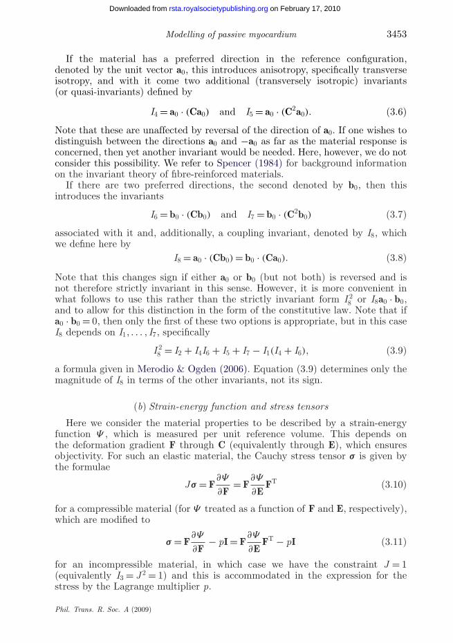
The passive myocardium tissue is an orthotropic material having threemutually orthogonal planes with distinct material responses, as the results ofDokos et al. (2002) from simple shear tests on passive ventricular myocardiumfrom pig hearts clearly show. This is illustrated in figure 2, which is based on fig. 6from the latter paper. It should be noted, however, that the ordering of the labelsfn and fs in fig. 6 of Dokos et al. (2002) is inconsistent with the data shown in theother figures in that paper. To correct this, we have switched the roles of fs andfn in figure 2 compared with fig. 6 of Dokos et al. (2002). This point is discussedfurther in §5d. The tissue exhibits a regionally dependent and time-dependent,highly nonlinear behaviour with relatively low hysteresis and also directionallydependent softening as the strain increases.
From figure 2, it can be seen that ventricular myocardium is least resistantto simple shear in the fn and sn planes for shear in the f and s directions,respectively (the lowest curve in figure 2 above the positive shear axis). It is
Phil. Trans. R. Soc. A (2009)
on February 17, 2010rsta.royalsocietypublishing.orgDownloaded from

3450 G. A. Holzapfel and R. W. Ogden
–0.5
0.3 0.50.1amount of shear
shea
r st
ress
(kP
a)
(nf ), (ns)(sn)
(sf )
(fn)
(fs)
–0.1–0.3 0
6
–6
12
–12
18
–18
Figure 2. Shear stress versus amount of shear for simple shear tests on a cube of a typical myocardialspecimen in the fs, fn and sn planes, where the (ij) shear refers to shear in the j direction in the ijplane, where i �= j ∈ {f, s, n}. Note that the (ij) shear entails stretching of material line elements thatare initially in the i direction. The data show clearly the distinct responses for the three planes andhence the orthotropy of the material. In addition, it illustrates the highly nonlinear response andthe viscoelastic effect evidenced by the relatively small hysteresis between loading and unloading.For the planes containing the f direction, the shear responses (fs) and (fn) in the s and n directionsare different; for the planes containing the s direction, the responses (sf) and (sn) in the f andn directions are also different; the shear responses (nf) and (ns) in the planes containing the ndirection are the same for the considered specimen. Adapted from Dokos et al. (2002).
most resistant to shear deformations that produce extension of the myocyte (f)axis in the fs and fn planes (the upper two curves for positive shear). Note,however, that for the planes containing the fibre direction, the shear responses(fs) and (fn) in the sheet and normal directions are different. Similarly, for theplanes containing the sheet direction, the responses (sf) and (sn) in the fibreand normal directions are different. On the other hand, the shear responsesin the planes containing the normal direction are the same for the consideredspecimen.
The passive biaxial mechanical properties of non-contracting myocardium aredescribed by Demer & Yin (1983), Yin et al. (1987), Smaill & Hunter (1991) andNovak et al. (1994), for example. To illustrate the results, we show in figure 3representative stress–strain data that we extracted from fig. 4 in Yin et al.(1987). For three different loading protocols for biaxial loading in the fs plane ofa canine left ventricle myocardium, figure 3a shows the second Piola–Kirchhoffstress Sff in the fibre direction as a function of the Green–Lagrange strain Effin the same direction, whereas figure 3b shows the corresponding plots for thesheet direction (Sss against Ess). The three sets of data in figure 3a,b correspondto constant strain ratios Eff/Ess. Just as for the shear response, the biaxial dataindicate high nonlinearity and anisotropy. Data for unloading were not given inYin et al. (1987).
Phil. Trans. R. Soc. A (2009)
on February 17, 2010rsta.royalsocietypublishing.orgDownloaded from

Modelling of passive myocardium 3451
0
2
4
6
8
10
12
14
16
18(a) (b)
S ff (
kPa)
0
2
4
6
8
10
12
0.05 0.10 0.15 0.20Ess
0.05 0.10 0.15 0.20Eff
S ss (
kPa)
Figure 3. Representative stress–strain data for three different loading protocols for biaxial loadingin the fs plane of canine left ventricle myocardium: (a) stress Sff against strain Eff in the fibredirection; (b) stress Sss against strain Ess in the sheet (cross-fibre) direction. Note that Eij andSij are the components of the Green–Lagrange strain tensor and the second Piola–Kirchhoff stresstensor, respectively. The three sets of data correspond to constant strain ratios Eff/Ess equal to2.05 (triangles), 1.02 (squares) and 0.48 (circles). The data are extracted from the two upper plotsin fig. 4 of Yin et al. (1987).
As with many other soft biological tissues, the myocardium can be regardedas an incompressible material. This has been established in experiments byVossoughi et al. (1980), who subjected tissue specimens to various levels ofhydrostatic stress. They recorded the associated volumetric strains and concludedthat the myocardial tissue is essentially incompressible.
According to experimental data obtained from equatorial slices of the leftventricular wall of potassium-arrested rat hearts, it is clear that the unloadedmyocardium is residually stressed (Omens & Fung 1990) and, in particular,that there is compressive circumferential residual stress in the endocardium ofthe left ventricle and tensile circumferential residual stress in the epicardium;see also Costa et al. (1997), who suggested that the residual stress in the leftventricle is associated with pre-stretching in the plane of the myocardial sheets.According to Costa et al. (1997), there is relatively little residual stress alongthe muscle fibre direction in the mid-wall and there are also residual stressesnormal to the fibre direction; the perimysial fibre network may be a primaryresidual stress-bearing structure in passive myocardium. Residual stresses arethought to arise during growth and remodelling (e.g. Rodriguez et al. 1994;Rachev 1997). Residual stresses have an important influence on the stress patternin the typical physiological state. For example, incorporation of a residual stressdistribution may reduce tensile endocardial stress concentrations predicted by
Phil. Trans. R. Soc. A (2009)
on February 17, 2010rsta.royalsocietypublishing.orgDownloaded from

3452 G. A. Holzapfel and R. W. Ogden
ventricular wall models (Guccione et al. 1991). The importance of residualstresses has also been recognized in arterial wall mechanics (e.g. Holzapfel et al.2000; Holzapfel & Ogden 2003). However, three-dimensional residual stressesare very difficult to quantify and hence their modelling must be treated withcaution.
Although the myocardium tissue appears to be viscoelastic, this aspect of itsbehaviour is not important from the point of view of mechanical modelling on thetime scale of the cardiac cycle, which is short compared with the relaxation timeof the viscoelastic response. Indeed, modelling of the viscoelasticity has receivedlittle attention in the literature, not least because there are very few data availableon the viscoelastic properties of the tissue. An exception to this is the model ofHuyghe et al. (1991). Here, we treat the tissue behaviour as elastic, with thecharacteristic features shown in figures 2 and 3.
It is therefore important to model the passive response of the left ventricularmyocardium as a non-homogeneous, thick-walled, incompressible, orthotropicnonlinearly elastic material, and this is the approach we adopt in the presentpaper. Although residual stresses are also important for the stress analysis ofthe composite myocardium, it is first necessary to develop a constitutive modelthat takes full account of the basic structure of the material with respect to astress-free reference configuration. Thus, we do not include residual stresses inthe constitutive model developed here, as was the case for the arterial modelconstructed in Holzapfel et al. (2000).
3. Essential elements of continuum mechanics
(a) Kinematical quantities and invariants
The basic deformation variable for the description of the local kinematics is thedeformation gradient F, and we use the standard notation and convention
J = det F > 0. (3.1)
For an incompressible material, we have the constraint
J = det F ≡ 1. (3.2)
Associated with F are the right and left Cauchy–Green tensors, defined by
C = FTF and B = FFT, (3.3)
respectively. Also important for what follows is the Green–Lagrange (or Green)strain tensor, defined by
E = 12(C − I), (3.4)
where I is the identity tensor. The principal invariants of C (and also of B) aredefined by
I1 = tr C, I2 = 12 [I 2
1 − tr (C2)] and I3 = det C, (3.5)
with I3 = J 2 = 1 for an incompressible material. These are isotropic invariants.For more details of the relevant material from continuum mechanics, we refer toHolzapfel (2000) and Ogden (1997).
Phil. Trans. R. Soc. A (2009)
on February 17, 2010rsta.royalsocietypublishing.orgDownloaded from
Modelling of passive myocardium 3453
If the material has a preferred direction in the reference configuration,denoted by the unit vector a0, this introduces anisotropy, specifically transverseisotropy, and with it come two additional (transversely isotropic) invariants(or quasi-invariants) defined by
I4 = a0 · (Ca0) and I5 = a0 · (C2a0). (3.6)
Note that these are unaffected by reversal of the direction of a0. If one wishes todistinguish between the directions a0 and −a0 as far as the material response isconcerned, then yet another invariant would be needed. Here, however, we do notconsider this possibility. We refer to Spencer (1984) for background informationon the invariant theory of fibre-reinforced materials.
If there are two preferred directions, the second denoted by b0, then thisintroduces the invariants
I6 = b0 · (Cb0) and I7 = b0 · (C2b0) (3.7)
associated with it and, additionally, a coupling invariant, denoted by I8, whichwe define here by
I8 = a0 · (Cb0) = b0 · (Ca0). (3.8)
Note that this changes sign if either a0 or b0 (but not both) is reversed and isnot therefore strictly invariant in this sense. However, it is more convenient inwhat follows to use this rather than the strictly invariant form I 2
8 or I8a0 · b0,and to allow for this distinction in the form of the constitutive law. Note that ifa0 · b0 = 0, then only the first of these two options is appropriate, but in this caseI8 depends on I1, . . . , I7, specifically
I 28 = I2 + I4I6 + I5 + I7 − I1(I4 + I6), (3.9)
a formula given in Merodio & Ogden (2006). Equation (3.9) determines only themagnitude of I8 in terms of the other invariants, not its sign.
(b) Strain-energy function and stress tensors
Here we consider the material properties to be described by a strain-energyfunction Ψ , which is measured per unit reference volume. This depends onthe deformation gradient F through C (equivalently through E), which ensuresobjectivity. For such an elastic material, the Cauchy stress tensor σ is given bythe formulae
Jσ = F∂Ψ
∂F= F
∂Ψ
∂EFT (3.10)
for a compressible material (for Ψ treated as a function of F and E, respectively),which are modified to
σ = F∂Ψ
∂F− pI = F
∂Ψ
∂EFT − pI (3.11)
for an incompressible material, in which case we have the constraint J = 1(equivalently I3 = J 2 = 1) and this is accommodated in the expression for thestress by the Lagrange multiplier p.
Phil. Trans. R. Soc. A (2009)
on February 17, 2010rsta.royalsocietypublishing.orgDownloaded from

3454 G. A. Holzapfel and R. W. Ogden
For an elastic material possessing a strain-energy function Ψ that depends ona list of invariants, say I1, I2, . . . , IN for some N , equations (3.10) and (3.11) maybe expanded in the forms
Jσ = FN∑
i=1
ψi∂Ii
∂Fand σ = F
N∑i=1,i �=3
ψi∂Ii
∂F− pI, (3.12)
respectively, where we have introduced the notation
ψi = ∂Ψ
∂Ii, i = 1, 2, . . . , N , (3.13)
with i = 3 omitted from the summation for the incompressible material andI3 omitted from the list of invariants in Ψ in this case. Note that ∂Ii/∂F =(∂Ii/∂E)FT in terms of the Green–Lagrange strain tensor. Note that the secondPiola–Kirchhoff stress tensor S, whose components were referred to in connectionwith figure 3, is given in terms of the Cauchy stress tensor via the simpleformula S = JF−1σF−T, using equation (3.10) for a compressible material andusing equation (3.11) for an incompressible material with J = 1. Explicitly, withE as the independent variable, we have simply
S = ∂Ψ
∂Eand S = ∂Ψ
∂E− p(I + 2E)−1 (3.14)
for compressible and incompressible materials, respectively.
4. Review of existing constitutive models
For references to early work concerned with constitutive modelling of themyocardium, we refer to papers by Yin (1981) and Humphrey & Yin (1987).Several of the earlier models were based on linear isotropic elasticity, which isentirely inappropriate in view of the discussion in §2b. Equally, the early nonlinearmodels do not capture all the features alluded to. This is the case for certaininvariant-based models, including the isotropic exponential form based on theinvariant I2 (Demiray 1976).
(a) Transversely isotropic models
A number of transversely isotropic models have been proposed. These includethe model of Humphrey & Yin (1987), which is the sum of two exponentials, onein I1 and one in I4, specifically
Ψ = c{exp[b(I1 − 3)] − 1} + A{exp[a(√
I4 − 1)2] − 1}, (4.1)
and contains four material parameters c, b, A and a. This was the firstanisotropic invariant-based model that took account of the fibre structure.Another transversely isotropic model, also based on the invariants I1 and I4,was constructed by Humphrey et al. (1990). This has the form
Ψ = c1(√
I4 − 1)2 + c2(√
I4 − 1)3 + c3(I1 − 3) + c4(I1 − 3)(√
I4 − 1) + c5(I1 − 3)2
(4.2)
Phil. Trans. R. Soc. A (2009)
on February 17, 2010rsta.royalsocietypublishing.orgDownloaded from

Modelling of passive myocardium 3455
and involves five material constants c1, c2, . . . , c5, values of which were obtainedby Novak et al. (1994) from biaxial test data from the middle portion of theinter-ventricular septum and the inner, middle and outer layers of the lateralpassive canine left ventricle wall. As discussed in §2, it only subsequentlybecame clear that the myocardium is not a transversely isotropic material (e.g.LeGrice et al. 1995).
The models referred to above are based on the assumption of incompressibility,but the shortcoming referred to above also applies to the compressible,transversely isotropic model due to Kerckhoffs et al. (2003), which has the form
Ψ = a0[exp(a1I 21 + a2I2) − 1] + a3[exp(a4E2
ff) − 1] + a5(I3 − 1)2, (4.3)
and contains six material parameters a0, a1, . . . , a5, where I1 and I2 are theprincipal invariants of E and Eff is the Green–Lagrange strain in the fibredirection. The invariants I1 and I2 are related to the principal invariants I1 andI2 of C defined in equation (3.5) by
I1 = 12(I1 − 3) and I2 = 1
4(I2 − 2I1 + 3). (4.4)
The first term in equation (4.3) represents the isotropic component relatedto tissue shape change, the second term relates to the extra stiffness of thematerial in the myofibre direction and finally the third term is related to volumechanges.
Other transversely isotropic models, based on the use of the components ofthe Green–Lagrange strain tensor, were developed by Guccione et al. (1991) andCosta et al. (1996), but again do not reflect the morphology discussed above.They are both special cases of the orthotropic model of Costa et al. (2001) to bediscussed below.
Some other models are structurally based. These include the model of Horowitzet al. (1988), which has the merit of being micro-mechanically motivated andinherently considers possible changes in the waviness of the fibres induced bythe tissue strain. On the other hand, because of the integrations involved in theconstitutive model, it is not well suited for numerical implementation. It is alsoeffectively transversely isotropic.
The paper by Huyghe et al. (1991) contains one of the few models thatcharacterize the passive viscoelastic response of the myocardium. It regards thematerial as sponge-like and treats it as a biphasic (fluid–solid) model based onthe quasi-linear viscoelastic constitutive model due to Fung (1993, §7.6) and, toour knowledge, is the only biphasic model of the myocardium documented in theliterature. The model has been implemented within a finite element frameworkand applied to the left ventricle of a canine diastolic heart in Huyghe et al.(1992). Of interest here is the solid elastic phase, which is a transversely isotropicmodel involving seven material parameters. However, the authors refer to it asorthotropic. That it is transversely isotropic can be seen from eq. (B 8) in appendixB of Huyghe et al. (1992) by noting that their strain-energy function is invariantunder interchange of the indices 1 and 2, and hence with respect to rotationsabout the 3 direction.
Phil. Trans. R. Soc. A (2009)
on February 17, 2010rsta.royalsocietypublishing.orgDownloaded from
3456 G. A. Holzapfel and R. W. Ogden
(b) Orthotropic models
Several orthotropic models have been proposed in the literature. Some of theseare inappropriate for modelling myocardial tissue, including the Langevin eight-chain based model of Bischoff et al. (2002), which, as pointed out by Schmid et al.(2008), does not reflect the morphology of the myocardium.
In the remainder of this section, we describe briefly three orthotropic modelsthat have similar features in that they are partly structurally based, relatingto the fibre, sheet and normal directions, and partly phenomenological. This is aprelude to the development, in §5, of a general orthotropic invariant-based model,which includes these three models as special cases.
Note that, in the models listed in §4b(i)–(iii) below, the authors have used thenotation Eij with i, j ∈ {f, s, n}, and, in particular, although Eij = Eji , they haveexpressed the off-diagonal terms in the form (Eij + Eji)/2, where i �= j . Here, forcompactness, we simply express this as Eij in each case.
(i) Strain-energy function proposed by Costa et al. (2001)
The Fung-type exponential strain-energy function due to Costa et al. (2001) isgiven by
Ψ = 12a(exp Q − 1), (4.5)
whereQ = bffE2
ff + bssE2ss + bnnE2
nn + 2bfsE2fs + 2bfnE2
fn + 2bsnE2sn, (4.6)
which has seven material parameters, a and bij , where i, j ∈ {f, s, n}.Interpretations were given for the parameters, but specific values were notprovided. As already mentioned, transversely isotropic specializations of thismodel (with five material parameters) were used in earlier papers by Guccioneet al. (1991) and Costa et al. (1996).
(ii) Fung-type model proposed by Schmid et al. (2006)
Another Fung-type model consisting of separate exponential terms for eachcomponent Eij was introduced by Schmid et al. (2006) to decouple the effects ofthe material parameters in the single-exponential model (4.5) and (4.6). With 12material parameters, it is given by
Ψ = 12aff [exp(bffE2
ff) − 1] + 12afn[exp(bfnE2
fn) − 1] + 12afs[exp(bfsE2
fs) − 1]+ 1
2ann[exp(bnnE2nn) − 1] + 1
2ans[exp(bnsE2ns) − 1] + 1
2ass[exp(bssE2ss) − 1].
(4.7)
We mention in passing another model with 12 parameters, which also usesthe components Eij , where i, j ∈ {f, s, n}. This is the tangent model introduced inSchmid et al. (2006); see also Schmid et al. (2008). We do not consider this modelhere.
(iii) Pole-zero model proposed by Hunter et al. (1997)
Motivated by the (equi-)biaxial tension tests of Smaill & Hunter (1991), Hunteret al. (1997) proposed the so-called pole-zero strain-energy function, which hasthe form
Phil. Trans. R. Soc. A (2009)
on February 17, 2010rsta.royalsocietypublishing.orgDownloaded from

Modelling of passive myocardium 3457
Ψ = kffE2ff
|aff − |Eff ||bff+ kfnE2
fn
|afn − |Efn||bfn+ knnE2
nn
|ann − |Enn||bnn
+ kfsE2fs
|afs − |Efs||bfs+ kssE2
ss
|ass − |Ess||bss+ knsE2
ns
|ans − |Ens||bns(4.8)
with 18 material parameters kij , aij and bij , where i, j ∈ {f, s, n}, and with differentcomponents Eij separated similarly to equation (4.7). As mentioned in Nash(1998), it was considered unlikely to be suitable for other modes of deformation.Note that several different forms of this model appear in various papers with orwithout appropriate modulus signs, and in some cases with bij set equal to 2 foreach i, j pair, as in Schmid et al. (2006, 2008).
The relative performance of the above orthotropic models in fitting data ofDokos et al. (2002) was evaluated in Schmid et al. (2008), and we discuss thisbriefly in §7.
5. A structurally based model for the passive myocardium
Bearing in mind the fibre, sheet (cross-fibre) and sheet-normal (normal) directionsspecified in figure 1e and the definition of the invariant I4 in the first part ofequation (3.6), we now consider the invariant I4 associated with each of thesedirections. We use the notation
I4 f = f0 · (Cf0), I4 s = s0 · (Cs0) and I4 n = n0 · (Cn0) (5.1)and note that ∑
i=f,s,n
I4 i = C : (f0 ⊗ f0 + s0 ⊗ s0 + n0 ⊗ n0) = C : I = I1. (5.2)
Thus, only three of the invariants I4 f , I4 s, I4 n and I1 are independent, and in thefunctional dependence of the strain energy we may omit one of these.
On the basis of the definition for the second part of equation (3.6), we may alsodefine invariants I5 f , I5 s and I5 n for each direction. We shall not need these here,but we note that they are related by I5 f + I5 s + I5 n = I 2
1 − 2I2. Additionally, thereare the coupling invariants associated with the pairs of directions. In accordancewith the definition (3.8), we may write
I8 fs = I8 sf = f0 · (Cs0), I8 fn = I8 nf = f0 · (Cn0) and I8 sn = I8 ns = s0 · (Cn0).(5.3)
In what follows, we shall make use of these. In fact, it is not difficult to show thatI5 f , I5 s and I5 n are expressible in terms of the other invariants via
I5 f = I 24 f + I 2
8 fs + I 28 fn, I5 s = I 2
4 s + I 28 fs + I 2
8 sn and I5 n = I 24 n + I 2
8 fn + I 28 sn
(5.4)and that
I4 fI4 sI4 n − I4 fI 28 sn − I4 sI 2
8 fn − I4 nI 28 fs + 2I8 fsI8 fnI8 sn = I3. (5.5)
Thus, if the material is compressible, there are seven independent invariants,whereas for an incompressible material there are only six. These numbers comparewith the eight (compressible) and seven (incompressible) for the case of a materialwith two non-orthogonal preferred directions. The orthogonality here reduces thenumber of invariants by one.
Phil. Trans. R. Soc. A (2009)
on February 17, 2010rsta.royalsocietypublishing.orgDownloaded from
3458 G. A. Holzapfel and R. W. Ogden
Note that, in terms of the components Eij , where i, j ∈ {f, s, n}, of the Green–Lagrange strain tensor used in several of the models discussed in §4, we have theconnections 2Eii = I4 i − 1, where i ∈ {f, s, n} (no summation over i), and 2Eij =I8 ij , where i �= j . Thus, the general framework herein embraces the orthotropicmodels discussed in §4 as special cases.
Before we consider the most general case, we note that, for a compressiblematerial that depends only on the invariants I1, I4 f , I4 s and I3, for example, thefirst formula in (3.12) yields
Jσ = 2ψ1B + 2ψ4 f f ⊗ f + 2ψ4 ss ⊗ s + 2I3ψ3I, (5.6)
where B = FFT, f = Ff0, s = Fs0 and ψ4 i = ∂Ψ/∂I4 i, where i = f, s. We shall also usethe notation n = Fn0. The counterpart of the formula (5.6) for an incompressiblematerial is
σ = 2ψ1B + 2ψ4 f f ⊗ f + 2ψ4 ss ⊗ s − pI. (5.7)
Note that here we have omitted the invariant I4 n rather than I1, I4 f or I4 s.There is a good physical reason for this choice, as we will explain in §6.
(a) Application to simple shear
Consider now simple shear in different planes and choose the axes so that thecomponent vectors are given by
[f0] = [1 0 0]T, [s0] = [0 1 0]T and [n0] = [0 0 1]T. (5.8)
We now consider simple shear separately in each of the three planes fs, sn andfn, and we identify the indices 1, 2 and 3 with f, s and n, respectively (figure 4).
(i) Shear in the fs plane
We begin with simple shear in the fs plane and consider separately shear inthe f0 and s0 directions. For shears in the f0 and s0 directions, the deformationgradients have components
[F] =[1 γ 00 1 00 0 1
]and [F] =
[1 0 0γ 1 00 0 1
], (5.9)
respectively. For the shear in the f0 direction, we obtain
[B] =⎡⎣1 + γ 2 γ 0
γ 1 00 0 1
⎤⎦ , f = f0, s = γ f0 + s0, n = n0, (5.10)
I4 s = 1 + γ 2, I4 f = I4 n = 1, the active shear stress is σ12 = 2γ (ψ1 + ψ4 s) andσ13 = σ23 = 0.
Phil. Trans. R. Soc. A (2009)
on February 17, 2010rsta.royalsocietypublishing.orgDownloaded from

Modelling of passive myocardium 3459
n0
f0
s0
f0
s0
f0
s0
(fs)(a) (c) (e)
(b) (d ) ( f )
n0 (sn) n0 (fn)
n0
f0
s0
f0
s0
f0
s0
(sf ) n0 (ns) n0 (nf )
Figure 4. Sketches of six possible modes of simple shear for myocardium defined with respect to thefibre axis f0, sheet axis s0 and sheet-normal axis n0: each mode is a plane strain deformation. Themodes are designated (ij), where i, j ∈ {f, s, n}, corresponding to shear in the ij plane with shear inthe j direction. Thus, the first letter in (ij) denotes the normal vector of the face that is shiftedby the simple shear, whereas the second denotes the direction in which that face is shifted. Themodes in which the fibres are stretched are (fn) and (fs).
For the shear in the s0 direction, we have
[B] =⎡⎣1 γ 0
γ 1 + γ 2 00 0 1
⎤⎦ , f = f0 + γ s0, s = s0, n = n0, (5.11)
I4 f = 1 + γ 2, I4 s = I4 n = 1, the active shear stress is σ12 = 2γ (ψ1 + ψ4 f) and againσ13 = σ23 = 0. Hence, the two shear responses in the fs plane are different. Notethat, for each of the above two cases, I8 fs = γ and I8 fn = I8 sn = 0.
(ii) Shear in the sn plane
Next, we consider simple shear in the sn plane, considering separately shearin the s0 and n0 directions. Shears in the s0 and n0 directions have deformationgradients with components
[F] =[1 0 00 1 γ0 0 1
]and [F] =
[1 0 00 1 00 γ 1
], (5.12)
Phil. Trans. R. Soc. A (2009)
on February 17, 2010rsta.royalsocietypublishing.orgDownloaded from

3460 G. A. Holzapfel and R. W. Ogden
respectively. For the shear in the s0 direction, we have
[B] =⎡⎣1 0 0
0 1 + γ 2 γ0 γ 1
⎤⎦ , f = f0, s = s0, n = n0 + γ s0, (5.13)
I4 n = 1 + γ 2, I4 f = I4 s = 1, the active shear stress is σ23 = 2γψ1 and σ12 = σ13 = 0.For the shear in the n0 direction, we obtain
[B] =⎡⎣1 0 0
0 1 γ
0 γ 1 + γ 2
⎤⎦ , f = f0, s = s0 + γn0, n = n0, (5.14)
I4 s = 1 + γ 2, I4 f = I4 n = 1, the active shear stress is σ23 = 2γ (ψ1 + ψ4 s) andσ12 = σ13 = 0. Hence, the two shear responses in the sn plane are different. Notethat, for each of the above two cases, I8 sn = γ and I8 fs = I8 fn = 0.
(iii) Shear in the fn plane
Finally, we have simple shear in the fn plane. For shears in the f0 and n0directions, the deformation gradients are
[F] =[1 0 γ0 1 00 0 1
]and [F] =
[1 0 00 1 0γ 0 1
], (5.15)
respectively. For the shear in the f0 direction, we have
[B] =⎡⎣1 + γ 2 0 γ
0 1 0γ 0 1
⎤⎦ , f = f0, s = s0, n = n0 + γ f0, (5.16)
I4 n = 1 + γ 2, I4 f = I4 s = 1, the active shear stress is σ13 = 2γψ1 and σ12 = σ23 = 0.For the shear in the n0 direction, we have
[B] =⎡⎣1 0 γ
0 1 0γ 0 1 + γ 2
⎤⎦ , f = f0 + γn0, s = s0, n = n0, (5.17)
I4 f = 1 + γ 2, I4 s = I4 n = 1, the active shear stress is σ13 = 2γ (ψ1 + ψ4 f) and σ12 =σ23 = 0. Hence, the two shear responses in the fn plane are different. Note that,for each of the above two cases, I8 fn = γ and I8 fs = I8 sn = 0.
Clearly, the (nf) and (ns) shear responses are the same, where we now recallthat we use the notation (ij) to specify that the shear is in the j direction in theij plane, with i, j ∈ {f, s, n}. In these two cases, there is stretching along the n0direction, but not along the f0 or s0 directions. The (sn) and (sf) shear responsesare also the same, with no stretching along the f0 or n0 direction and, finally, theresponses are also the same in the fs and fn planes, with stretching along thefibre direction f0 in these cases. It should also be emphasized that, in the above,the order of the indices i and j in (ij) (when referring to shear or response) isimportant, but without parentheses, in ij , the order is not relevant (when referringto plane).
Phil. Trans. R. Soc. A (2009)
on February 17, 2010rsta.royalsocietypublishing.orgDownloaded from

Modelling of passive myocardium 3461
The data of Dokos et al. (2002) indicate that the shear response is stiffestwhen the fibre direction is extended, least stiff when the normal direction isextended and has intermediate stiffness when the sheet direction is extended.This is reflected by the above formulae for the shear stresses if ψ4 f > ψ4 s > 0.However, the data also show that there are differences between the (fs) and (fn)and between the (sf) and (sn) responses, which are not captured by the abovemodel; the data also show that the (nf) and (ns) responses are indistinguishable.A possible way to refine the model in order to reflect these differences is to includein the strain-energy function one or more of the coupling invariants defined inequation (5.3). Bearing in mind that the most general strain-energy functiondepends only on seven invariants for a compressible material, we may select, forexample, I1, I2, I3, I4 f , I4 s, I8 fs and I8 fn, in which case the Cauchy stress (5.6) isgiven by
Jσ = 2ψ1B + 2ψ2(I1B − B2) + 2I3ψ3I + 2ψ4 f f ⊗ f + 2ψ4 ss ⊗ s+ ψ8 fs(f ⊗ s + s ⊗ f ) + ψ8 fn(f ⊗ n + n ⊗ f ). (5.18)
We emphasize that the invariants I8 fs and I8 fn appearing in equation (5.18), andalso I8 sn, depend on the sense of f0, s0 and n0, i.e. they change sign if the senseof one of the vectors is reversed. However, Ψ should be independent of this senseand this is accommodated by an appropriate functional dependence. For example,if we write Ψ (. . . , I 2
8 fs, . . .) = Ψ (. . . , I8 fs, . . .), then ψ8 fs = 2∂Ψ /∂(I 28 fs)I8 fs and for
shear in the fs plane we have I8 fs = f · s = γ for either direction of shear, and thisvanishes in the reference configuration, as does ψ8 fs provided Ψ is well behavedas a function of I 2
8 fs (which we assume to be the case). Similarly, I8 fn = f · n = γfor shear in the fn plane and I8 sn = s · n = γ for shear in the sn plane.
In view of the above, in the reference configuration, equation (5.18) reduces to
2(ψ1 + 2ψ2 + ψ3)I + 2ψ4 f f0 ⊗ f0 + 2ψ4 ss0 ⊗ s0 = 0, (5.19)
assuming the reference configuration is stress-free, and this can hold only if
ψ1 + 2ψ2 + ψ3 = 0, ψ4 f = 0 and ψ4 s = 0. (5.20)
Thus, these conditions must be satisfied along with
ψ8 fs = ψ8 fn = 0 (5.21)
in the reference configuration.For an incompressible material, equation (5.18) is replaced by
σ = 2ψ1B + 2ψ2(I1B − B2) − pI + 2ψ4 f f ⊗ f + 2ψ4 ss ⊗ s+ ψ8 fs(f ⊗ s + s ⊗ f) + ψ8 fn(f ⊗ n + n ⊗ f) (5.22)
and only the six invariants I1, I2, I4 f , I4 s, I8 fs and I8 fn remain. In this case, theconditions that must be satisfied in the reference configuration are as above exceptfor the first equation in (5.20), which is replaced by 2ψ1 + 4ψ2 − p0 = 0, where p0is the value of p in the reference configuration.
Phil. Trans. R. Soc. A (2009)
on February 17, 2010rsta.royalsocietypublishing.orgDownloaded from

3462 G. A. Holzapfel and R. W. Ogden
For simple shear in the fs plane, the term in ψ8 fs contributes ψ8 fs to σ12 forshear in either the f0 or s0 direction, but does not contribute if the shear is ineither the fn or sn plane. Similarly, the term in ψ8 fn contributes ψ8 fn to σ13 forshear in either the f0 or n0 direction in the fn plane. Also, as noted above, becausethe dependence of Ψ is on the square of each of these invariants, each of thesetwo terms involves a factor of γ .
In summary, the equations for shear stress versus amount of shear for the sixsimple shears enumerated in §5a(i)–(iii) are given by
(fs): σfs = 2(ψ1 + ψ2 + ψ4 f)γ + ψ8 fs, (5.23)
(fn): σfn = 2(ψ1 + ψ2 + ψ4 f)γ + ψ8 fn, (5.24)
(sf): σfs = 2(ψ1 + ψ2 + ψ4 s)γ + ψ8 fs, (5.25)
(sn): σsn = 2(ψ1 + ψ2 + ψ4 s)γ , (5.26)
(nf): σfn = 2(ψ1 + ψ2)γ + ψ8 fn (5.27)
and (ns): σsn = 2(ψ1 + ψ2)γ . (5.28)
It is worth remarking here that, as simple shear is a plane strain deformation,the invariants I1 and I2 are identical and the effects of ψ1 and ψ2 cannot bedistinguished.
(b) Application to biaxial deformation
Several experiments have been conducted using biaxial tests on thin sheetsof tissue taken from planes parallel to the endocardium. Such specimens arepurportedly from within a sheet containing the fibre axis and the in-sheet axis.These are referred to as the fibre and cross-fibre directions. Note, however, that,according to the structure discussed in §2, such specimens are, in general, unlikelyto contain a specific myocyte sheet, so care must be exercised in interpreting suchbiaxial data.
Consider the pure homogeneous deformation defined by
x1 = λfX1, x2 = λsX2 and x3 = λnX3, (5.29)
where λf , λs and λn are the principal stretches, identified with the fibre, sheet andnormal directions, respectively. They satisfy the incompressibility condition
λfλsλn = 1. (5.30)
When the deformation (5.29) is applied to a thin sheet of tissue parallel toa sheet with no lateral stress, there is no shear strain and hence I8 ij = 0, wherei �= j ∈ {f, s, n}, and ψ8 ij = 0 correspondingly. Equation (5.22) then has only threecomponents, namely
σff = 2ψ1λ2f + 2ψ2(λ
2s + λ2
n)λ2f + 2ψ4 fλ
2f − p, (5.31)
σss = 2ψ1λ2s + 2ψ2(λ
2n + λ2
f )λ2s + 2ψ4 sλ
2s − p (5.32)
and 0 = 2ψ1λ2n + 2ψ2(λ
2f + λ2
s )λ2n − p. (5.33)
Phil. Trans. R. Soc. A (2009)
on February 17, 2010rsta.royalsocietypublishing.orgDownloaded from
Modelling of passive myocardium 3463
Elimination of p by means of equation (5.33) allows equations (5.31) and (5.32)to be expressed as
σff = 2ψ1(λ2f − λ2
n) + 2ψ2λ2s (λ
2f − λ2
n) + 2ψ4 fλ2f (5.34)
and σss = 2ψ1(λ2s − λ2
n) + 2ψ2λ2f (λ
2s − λ2
n) + 2ψ4 sλ2s . (5.35)
If we omit the dependence on the invariant I2, then the last two equationssimplify to
σff = 2ψ1(λ2f − λ2
n) + 2ψ4 fλ2f (5.36)
and σss = 2ψ1(λ2s − λ2
n) + 2ψ4 sλ2s . (5.37)
(c) A specific model
To decide which of the invariants to include in a particular model, wenow examine interpretations of the invariants. First, we include an isotropicterm based on the invariant I1 because this can be regarded as associatedwith the underlying non-collagenous and non-muscular matrix (which includesfluids). This could be modelled as a neo-Hookean material, as in the caseof arteries (Holzapfel et al. 2000), or as an exponential (Demiray 1972),for example.
A schematic of the embedded collagen–muscle fibre structure is shown infigure 5 for the unloaded configuration and, separately, for configurations subjectto tension and compression in the direction of the muscle fibre (cardiac myocyte).The collagen fibres illustrated in figure 5 are thought to represent both theendomysial and the perimysial collagen fibres, as briefly described in §2a.Figure 5b, in particular, shows the configuration in which the tensile loadingis in the muscle fibre direction. The muscle fibres are extended and the inter-fibre distances are decreased, while the collagenous network offers little resistancelaterally but does contribute to the exponentially increasing stress in the musclefibre direction. For tensile loading lateral to the muscle fibres, there is alsoexponential stress stiffening, which can be thought of as being generated byrecruitment of the collagen network. Figure 5c depicts the tendency of the musclefibres to buckle under compressive load in the muscle fibre direction and stretchedcollagen cross-fibres, i.e. the lateral inter-fibre connections as well as the wovenperimysial network are stretched. It is suggested that the lateral stretching of thecollagen fibres contributes to the observed, relatively high compressive stiffnessof the myocardium.
To reflect the stiffening behaviour in the muscle fibre direction, as shown byexperimental tests (e.g. figures 2 and 3), it is appropriate to use an exponentialfunction of I4 f . Similarly, for the sheet direction, transverse to the muscle fibres;in this direction, the stiffening is in part associated with the collagen fibresconnecting the muscle fibres, as discussed above. For this direction, we usean exponential function of the invariant I4 s. Clearly, these terms contributesignificantly to the stored energy when the associated directions are under tension.However, when they are under compression, their contribution is minimal becausethe fibres do not support compression. For this reason, we include these terms in
Phil. Trans. R. Soc. A (2009)
on February 17, 2010rsta.royalsocietypublishing.orgDownloaded from

3464 G. A. Holzapfel and R. W. Ogden
collagen fibre
muscle fibre
unloaded(a)
matrix
tension(b)
compression(c)
Figure 5. Schematic of the arrangement of muscle and collagen fibres and the surrounding matrix:(a) unloaded structure; (b) structure under tensile load in the muscle fibre direction, showingdecreased inter-fibre separation so that the collagen network bears load primarily in the musclefibre direction; (c) structure under compressive load in the muscle fibre direction, showing themuscle fibres buckled and lateral extension of the collagen network.
the energy function only if I4 f > 1 or I4 s > 1, as appropriate. As I4 n depends on I1,I4 f and I4 s, we do not include it separately and therefore tensile and compressivebehaviour in the normal direction is accommodated by the term in I1. These threeinvariants are sufficient to model the tension/compression behaviour, and thereis no need to include I2. Indeed, they are also sufficient to characterize the basicfeatures of the shear test results of Dokos et al. (2002), which we will demonstratein the following section.
As far as the more detailed shear behaviour is concerned (figure 2), it isnecessary to make use of one or more of the invariants I8 ij . In view of theexponential trends shown in figure 2, particularly for the curves (fs) and (fn), wechoose to use an exponential function also for this part of the characterization.In particular, as the (nf) and (ns) curves are not distinguished (figure 2), it turnsout that we need to consider only the invariant I8 fs associated with stretching ofthe fibres, and not I8 fn or I8 sn. The above considerations lead us to propose theenergy function given by
Ψ = a2b
exp[b(I1 − 3)] +∑i=f,s
ai
2bi
{exp[bi(I4 i − 1)2] − 1
} + afs
2bfs
[exp(bfsI 2
8 fs) − 1],
(5.38)
Phil. Trans. R. Soc. A (2009)
on February 17, 2010rsta.royalsocietypublishing.orgDownloaded from

Modelling of passive myocardium 3465
0
2
4
6
8
10
12
14
16
0.1 0.2 0.3amount of shear
0.4
(nf ), (ns)
(sn)
(sf )
(fn)
(fs)
0.5 0.6
shea
r st
ress
(kP
a)
Figure 6. Fit of the model (5.39) with the final term omitted (full curves) to the experimental data(circles) for the loading curves from figure 2: (nf)–(ns) and mean of the loading curves for (fs) and(fn) and for (sf) and (sn). The material parameters used are given in table 1.
where a, b, af , as, bf , bs, afs and bfs are eight positive material constants,the a parameters having dimension of stress, whereas the b parameters aredimensionless. This consists of the isotropic term in I1, the transversely isotropicterms in I4 f and I4 s and the orthotropic term in I8 fs. Note that, if we do notdistinguish between the (fs) and (fn) and between the (sf) and (sn) responses,then only six constants are needed.
From equation (5.22), this yields the Cauchy stress
σ = a exp[b(I1 − 3)]B − pI + 2af(I4 f − 1) exp[bf(I4 f − 1)2]f ⊗ f
+ 2as(I4 s − 1) exp[bs(I4 s − 1)2]s ⊗ s + afsI8 fs exp(bfsI 28 fs)(f ⊗ s + s ⊗ f ).
(5.39)
In the following section, we apply this specific strain-energy function to bothbiaxial and shear test data and discuss the results in detail.
(d) Fit of the Yin et al. (1987) and Dokos et al. (2002) data
In this section, we show the efficacy of the proposed model for fitting data onthe myocardium. First, we use the simplified model based on the three invariantsI1, I4 f and I4 s for which the Cauchy stress is given by equation (5.39) with the finalterm omitted. The resulting fit with the mean of the loading curves for positive(fs) and (fn) and for positive (sf) and (sn) shears, as well as the common curvefor positive (nf) and (ns) shears, extracted from figure 2, is shown in figure 6.
Phil. Trans. R. Soc. A (2009)
on February 17, 2010rsta.royalsocietypublishing.orgDownloaded from
3466 G. A. Holzapfel and R. W. Ogden
00
2
4
6
8
10
12
14
16
0.1 0.2 0.3amount of shear
0.4 0.5 0.6
shea
r st
ress
(kP
a)
(nf ), (ns)
(sn)
(sf )
(fn)
(fs)
Figure 7. Fit of the model (5.39) (full curves) to the experimental data (circles) for the loadingcurves from figure 2 with separate (fs), (fn), (sf), (sn) and (nf)–(ns) not distinguished. The materialparameters used are given in table 1.
Clearly, this simple model reflects the general characteristics of the distinct shearsin the different directions, which exemplify the orthotropy. It is also worth notingthat, if the isotropic term is replaced by the neo-Hookean term μ(I1 − 3)/2, thefit is still relatively good, although the shear stress versus amount of shear is thenlinear for the (nf)–(ns) plot. We do not show this plot. The data shown in figure2 indicate that the response for negative shears is very similar to that for positiveshear (with reversed sign of the amount of shear and shear stress). Fitting thenegative shear data along with those for positive shear would have a minor effecton the values of the fitting parameters.
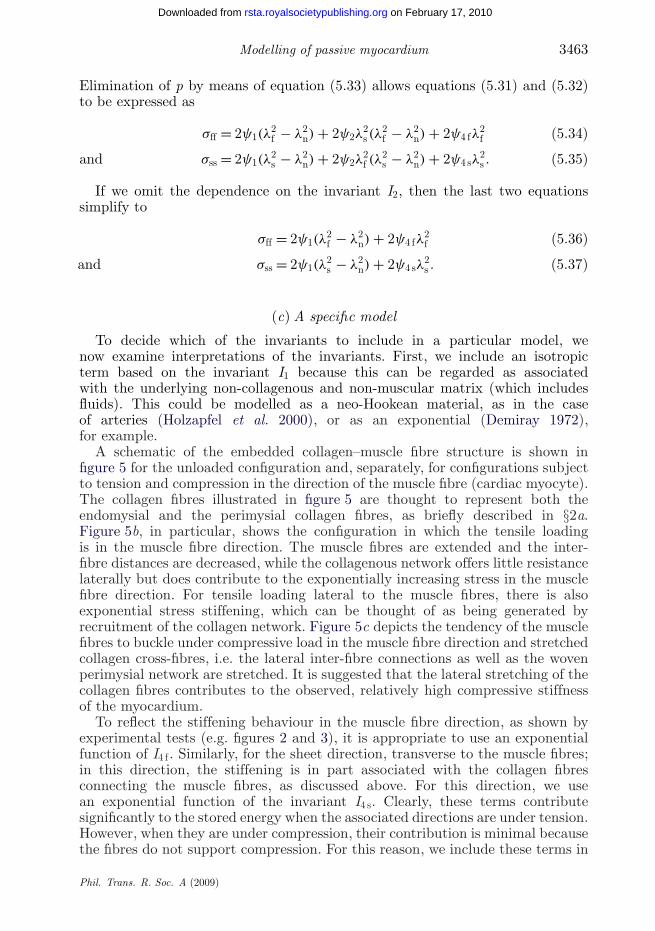
Second, with this as a starting point, we now refine the fitting by including thefinal term in equation (5.39), which allows the (fs) and (fn) and the (sf) and (sn)plots to be separated according to figure 2. The resulting fit is shown in figure 7and indicates very good agreement between the model and the experimental data.As mentioned in §2b, we have reversed the labels fn and fs compared with thosein Dokos et al. (2002). This is because all the other curves in the latter papershow that the (fs) shear response is stiffer than that for (fn). This indeed makessense because the stiffnesses in the f, s and n directions are, as noted previously,ordered according to f > s > n. Thus, the (fs) shear response is expected to bestiffer than the (fn) response. Equally, the (sf) response is stiffer than the (sn)response. It is also suggested that the (nf) response should be stiffer than the(ns) response, although there is no clear distinction seen in figure 2. Other datashown in Dokos et al. (2002) do indeed show a small separation in the sense justindicated. The values of the material parameters for the fits shown in figures 6and 7 are summarized in table 1.
Phil. Trans. R. Soc. A (2009)
on February 17, 2010rsta.royalsocietypublishing.orgDownloaded from

Modelling of passive myocardium 3467
0
2
4
6
8
10
12
14
16
18(a) (b)S ff
(kP
a)
0
2
4
6
8
10
12
0.05 0.10 0.15 0.20Ess
0.05 0.10 0.15 0.20Eff
S ss (
kPa)
Figure 8. Fit of the model (5.39) to the experimental data of figure 3 (extracted from Yin et al.1987) for three different loading protocols for biaxial loading in the fs plane: (a) stress Sff againststrain Eff in the fibre direction; (b) stress Sss against strain Ess in the sheet (cross-fibre) direction.The three sets of experimental data correspond to constant strain ratios Eff/Ess equal to 2.05(triangles), 1.02 (squares) and 0.48 (circles), whereas the full curves represent the fitted model.The biaxial data can be captured by a transversely isotropic model, and hence only four materialconstants are required to fit the data. The material parameters used are given in table 1.
Table 1. Material parameters a, b, af , bf , as, bs, afs and bfs for the energy function (5.38) used tofit the simple shear data for myocardium (Dokos et al. 2002) in figures 6 and 7 and the biaxialtension data (Yin et al. 1987) in figure 8.
a af as afsexperimental data (kPa) b (kPa) bf (kPa) bs (kPa) bfs
shear, figure 6 0.057 8.094 21.503 15.819 6.841 6.959 — —shear, figure 7 0.059 8.023 18.472 16.026 2.481 11.120 0.216 11.436biaxial, figure 8 2.280 9.726 1.685 15.779 — — — —
Next, we use the model (5.39), specialized for the biaxial mode of deformationaccording to equations (5.36) and (5.37), to fit the experimental data obtainedfrom Yin et al. (1987) and shown in figure 8. The associated material parametersare summarized in the last row of table 1.
We are using here the biaxial data of Yin et al. (1987) for illustrationpurposes because, to our knowledge, they are the only true biaxial, as distinctfrom equibiaxial, data available. However, these data have limitations and, inparticular, it should be noted that they do not provide information in thelow-strain region (between 0 and 0.05). This highlights the need for more complete
Phil. Trans. R. Soc. A (2009)
on February 17, 2010rsta.royalsocietypublishing.orgDownloaded from

3468 G. A. Holzapfel and R. W. Ogden
biaxial data. The fit presented in figure 8 is therefore rather crude but canbe improved if required by changing the isotropic term, i.e. the I1 function,and/or by including an activation threshold to accommodate the ‘toe’ region.Whether or not this is done, it is important to recognize that the biaxial data ofYin et al. (1987) can be captured by a transversely isotropic specialization of themodel. For the model used here, as can be seen from table 1, only four materialconstants (with as = 0) are required. Hence, the biaxial data alone appear tosuggest that the material is transversely isotropic. As this conflicts sharply withthe shear data, care must be taken in drawing conclusions from biaxial dataalone. Additional experimental tests are required. For a fuller discussion of thetheory underpinning planar biaxial tests for anisotropic nonlinearly elastic solids,we refer to Holzapfel & Ogden (in press).
6. Convexity and related issues
Holzapfel et al. (2000) discussed the important issue of convexity of thestrain-energy function and its role in ensuring material stability and physicallymeaningful and unambiguous mechanical behaviour. It is also important forfurnishing desirable mathematical features of the governing equations that have,in particular, implications for numerical computation; see also Ogden (2003,2009) and Holzapfel et al. (2004) for further discussion of convexity and relatedinequalities. For the discussion here, the form of the strain-energy function(5.38) has particular advantages because it is the sum of separate functionsof different invariants, with no cross-terms between the invariants involved.This enables the convexity status of each term to be assessed separately. Weshall, therefore, consider in succession the three functions F (I1), G(I4 f) andH(I8 fs) as representatives and examine their convexity as a function of the rightCauchy–Green tensor C.
(a) The function F (I1)
First we note that
∂F (I1)
∂C= F ′(I1)I and
∂2F (I1)
∂C ∂C= F ′′(I1)I ⊗ I. (6.1)
Local convexity of F (I1) as a function of C requires that
∂2F (I1)
∂C ∂C[A, A] ≡ F ′′(I1)(tr A)2 ≥ 0 (6.2)
for all second-order tensors A, from which we deduce that F ′′(I1) ≥ 0. Note thatstrict convexity is not possible because A can be chosen so that tr A = 0. For theexponential function considered in equation (5.38), i.e.
F (I1) = a2b
{exp[b(I1 − 3)] − 1}, (6.3)
this yields ab ≥ 0. For a non-trivial function, however, we must have ab > 0. Itis also easy to see that, for the stress response (in simple tension, for example)to be exponentially increasing in the corresponding stretch, we must have b > 0.Thus, we have a > 0 and b > 0.
Phil. Trans. R. Soc. A (2009)
on February 17, 2010rsta.royalsocietypublishing.orgDownloaded from

Modelling of passive myocardium 3469
(b) The function G(I4 f)
For G(I4 f), it follows from the definition of I4 f in equation (5.1) that
∂G∂C
= G′(I4 f)f0 ⊗ f0 and∂2G
∂C ∂C= G′′(I4 f)f0 ⊗ f0 ⊗ f0 ⊗ f0. (6.4)
Local convexity of G(I4 f) requires that
∂2G∂C∂C
[A, A] ≡ G′′(I4 f) [(Af0) · f0]2 ≥ 0 (6.5)
for all second-order tensors A. It follows that G is convex in C provided G′′(I4 f) ≥ 0.For the exponential form
G(I4 f) = af
2bf{exp[bf(I4 f − 1)2] − 1}, (6.6)
we obtain
G′(I4 f) = af(I4 f − 1) exp[bf(I4 f − 1)2] (6.7)
and G′′(I4 f) = af exp[bf(I4 f − 1)2]{1 + 2bf(I4 f − 1)2}. (6.8)
For extension in the fibre direction, we have I4 f > 1, and from equation (6.7)we deduce that for the material response associated with this term to stiffen inthe fibre direction we must have af > 0 and bf > 0. Moreover, these inequalitiesimply that G′′(I4 f) > 0 and hence G is a convex function (both in tension and incompression). It can be shown similarly that the separable Fung-type model (4.7)is convex if the material constants it contains are positive.
As the pole-zero model (4.8) is separable it can be treated on the same basis.For example, if we consider just the first term in equation (4.8), we may write
G(I4 f) = kffE2ff
|aff − |Eff | |bff, (6.9)
where I4 f = 1 + 2Eff and, with kff > 0, aff > 0 and bff > 0, it is straightforward toshow that this is convex for all Eff if 0 < bff ≤ 1 or bff ≥ 2. However, it is convexfor all Eff such that |Eff | < aff (which is a necessary restriction) irrespective of thevalue of bff > 0.
Although the calculations are somewhat different (because the contributionsof the different components Eij are not separable), it is also easily shown thatthe Costa model (4.5) and (4.6) and similar Fung-type models are convex if thecoefficients bij are positive. By contrast, some models are not, in general, convex,as is the case with model (4.2) because of the influence of the term cubic in√
I4 − 1 and the coupled term in I1 and I4.
Phil. Trans. R. Soc. A (2009)
on February 17, 2010rsta.royalsocietypublishing.orgDownloaded from
3470 G. A. Holzapfel and R. W. Ogden
(c) The function H(I8 fs)
Similar results hold for H(I8 fs). Using the first term in definition (5.3), wecalculate
∂H∂C
= 12H′(I8 fs)(f0 ⊗ s0 + s0 ⊗ f0) (6.10)
and∂2H
∂C ∂C= 1
4G′′(I8 fs)(f0 ⊗ s0 + s0 ⊗ f0) ⊗ (f0 ⊗ s0 + s0 ⊗ f0). (6.11)
For an arbitrary second-order tensor A, we have
∂2H∂C ∂C
[A, A] ≡ H′′(I8 fs)[(Af0) · s0]2 (6.12)
and for convexity this must be non-negative for all A. Thus, H is convex in Cprovided H′′(I8 fs) ≥ 0.
For the exponential form
H(I8 fs) = afs
2bfs[exp(bfsI 2
8 fs) − 1], (6.13)
we obtain
H′′(I8 fs) = afs exp[bfs(I8 fs − 1)2](1 + 2bfsI 28 fs), (6.14)
so convexity is guaranteed if afs > 0 and bfs > 0.In the above discussion based separately on the invariants I1, I4 f and I8 fs, we
have examined only the convexity of individual terms that contribute (additively)to the strain-energy function. If each such term is convex, then the overall strain-energy function is convex. Note, however, that it is not necessary that each suchcontribution be convex provided any non-convex contribution is counterbalancedby the convexity of the other terms. The analysis of convexity is relativelystraightforward for a compressible material, but for an incompressible materialmore care is needed because then not all components of E are independent. Fordiscussion of different aspects of convexity, see Holzapfel et al. (2000) and Ogden(2003, 2009).
(d) Strong ellipticity and other inequalities
The notion of convexity is different from, but closely related to, aspects ofmaterial stability, for discussions of which in the context of the mechanics ofsoft biological tissues we refer to Holzapfel et al. (2004) and Ogden (2003,2009), for example, and references therein. Whether or not the strong ellipticitycondition holds is one issue that arises in consideration of material stability. Ifit holds, then the emergence of certain types of non-smooth deformations, forexample, is precluded. For three-dimensional deformations, analysis of the strongellipticity condition is difficult, especially for anisotropic materials such as thoseconsidered here. Necessary and sufficient conditions for strong ellipticity to holdfor isotropic materials are available for three dimensions but are very complicated;in two dimensions, they are much more transparent, but their counterparts,even for transversely isotropic materials, are not available. For plane straindeformations, the strong ellipticity condition has been analysed in some detail
Phil. Trans. R. Soc. A (2009)
on February 17, 2010rsta.royalsocietypublishing.orgDownloaded from
Modelling of passive myocardium 3471
by Merodio & Ogden (2002, 2003) for incompressible and compressible fibre-reinforced elastic materials. Here we focus our brief discussion on the anisotropiccontributions to the strain-energy function.
If we consider the term G(I4 f), for example, on its own, then (Merodio & Ogden2002) strong ellipticity requires that the inequalities
G′(I4 f) + 2I4 fG′′(I4 f) > 0 and G′(I4 f) > 0 (6.15)
hold. From equation (5.22) and the formula f · f = I4 f , which comes from the firstequation in (5.1), it can be seen that the component of Cauchy stress in thefibre direction is given by 2I4 fG′(I4 f). For this to be positive (negative) whenI4 f > 1 (< 1), we require G′(I4 f) > 0 (< 0), which means that strong ellipticity doesnot hold under fibre compression (this is the case for the exponential model; seeequation (6.7)). In the context of arterial wall mechanics (Holzapfel et al. 2000),this problem is circumvented by recognizing that the fibres tend to buckle incompression and do not support compression to a significant degree, so that theterm G(I4 f) can be considered to be inactive when I4 f < 1. Even if this termis not dropped for compression in the fibre direction, its tendency to lead toloss of ellipticity is moderated to some extent by the other terms in the strain-energy function. Turning now to the first inequality in (6.15), we note that this isequivalent to requiring that the nominal stress component in the fibre direction bea monotonic function of the stretch
√I4 f in that direction, as shown by Merodio &
Ogden (2002), which is consistent with the typical stiffening of the stress responseof the fibres.
The situation with regard to H(I8 fs) is more delicate because, on its own,it can violate strong ellipticity in either tension or compression and generallyhas a destabilizing influence (Merodio & Ogden 2006). Here we examine itsbehaviour for simple shear. With reference to equation (5.22), we note that H(I8 fs)contributes the term H′(I8 fs)(f ⊗ s + s ⊗ f ) to the Cauchy stress σ. For the simpleshear (sf) in the fs plane, we have f = f0 and s = γ f0 + s0, where I8 fs = γ is theamount of shear (see §5a(i)). The component of the shear stress on the planenormal to the initial direction s0 is then simply σ12 = H′(I8 fs) and we require
H′(γ ) � 0 as γ � 0 (6.16)
for the shear stress and strain to be in the same direction. Furthermore, ifwe require σ12 to be a monotonic increasing function of γ , then we must haveH′′(I8 fs) ≥ 0, which is consistent with the requirement of convexity in §6c.
7. Discussion
To understand the highly nonlinear mechanics of the complex structure ofthe passive myocardium under different loading regimes, a rationally basedcontinuum model is essential. In the literature to date, models of the myocardiumhave been mainly of polynomial and/or exponential form, an important exceptionbeing the pole-zero model (4.8). Many of the models, including recently publishedones, have been based on the assumption of transverse isotropy and are nottherefore able to capture the orthotropic response illustrated in the shear data ofDokos et al. (2002) on the myocardium. Moreover, not all of these are consistentwith convexity requirements noted in §6; an example of such is equation (4.2), as
Phil. Trans. R. Soc. A (2009)
on February 17, 2010rsta.royalsocietypublishing.orgDownloaded from

3472 G. A. Holzapfel and R. W. Ogden
mentioned in §6. As for the orthotropic models presented in §4b, we have alreadynoted the common feature that they are expressed in terms of the componentsof the Green–Lagrange strain tensor and that these particular components arealso expressible in terms of the invariants. Thus, they all fit within the generalframework we have outlined in §5. Note, however, that none of them has anexplicit isotropic contribution.
Although the Costa et al. (2001) model (4.5) and (4.6) has seven materialparameters, the model (4.7) has 12 and the pole-zero model in its most generalform (4.8) has 18. However, the first of these three models has the disadvantagethat the parameters are highly coupled and hence difficult to interpret in terms ofthe myocardium structure. As pointed out by Schmid et al. (2008), the parameterestimation process for the strain-energy function of Costa et al. (2001) wasreliable, whereas for equation (4.7) and the special case of equation (4.8) with 12parameters the process was unstable and required more sophisticated strategies,as outlined in their paper. It should be pointed out that, in general, least-squaresoptimization procedures with large numbers of parameters can lead to non-uniqueness of parameter sets because of sensitivity to small changes in the data(e.g. Fung 1993, §8.6.1). Another common feature is that the orthotropic modelsreviewed here are somewhat ad hoc in nature and were constructed without thebenefit of the general underlying theory such as that described in §5. Nevertheless,in spite of some shortcomings, including lack of convexity in some cases, thesemodels have certainly been helpful in establishing some understanding of thebiomechanics of the myocardium.
The specific constitutive model proposed in equation (5.38) has been shown todescribe the general characteristics of the available biaxial data relatively well andto fit the available shear data very well. This is a model with only four invariantsthat is included within the general framework based on six independent invariantsfor an incompressible orthotropic material, which the myocardium is considered tobe. A particular merit of the invariant theory is that it is geometry independentand requires knowledge only of the local preferred directions in the material.Moreover, it is relatively easy to implement within a finite element environment,as is the case with the invariant-based models for arteries (e.g. Holzapfel 2000).The three-dimensional orthotropic model is based on a structural approach inthat it takes account of the morphological structure through the muscle fibredirection, the myocyte sheet orientation and the sheet normal direction andconsiders the resulting macroscopic nature of the myocardium. In this sense,it is not considered to be a micro-mechanically based model. The particularform of the model adopted here uses a set of eight material parameters whoseinterpretations can be based partly on the underlying histology. This number canbe reduced to five if the neo-Hookean model is used as the isotropic term forfitting the biaxial data or for illustrating basic features of the different simpleshear modes. Construction of the model has been greatly facilitated by the clearstructure of the stress–deformation equations that follow from the general form(5.22) and its specializations such as equations (5.23)–(5.28). Furthermore, themodel introduced here is consistent with standard inequalities required fromconsiderations of convexity, strong ellipticity and material stability.
Although some aspects of the passive mechanical response of the myocardiumseem to be well known, a careful literature survey shows that there are insufficientexperimental data available, and there is therefore a pressing need for more
Phil. Trans. R. Soc. A (2009)
on February 17, 2010rsta.royalsocietypublishing.orgDownloaded from
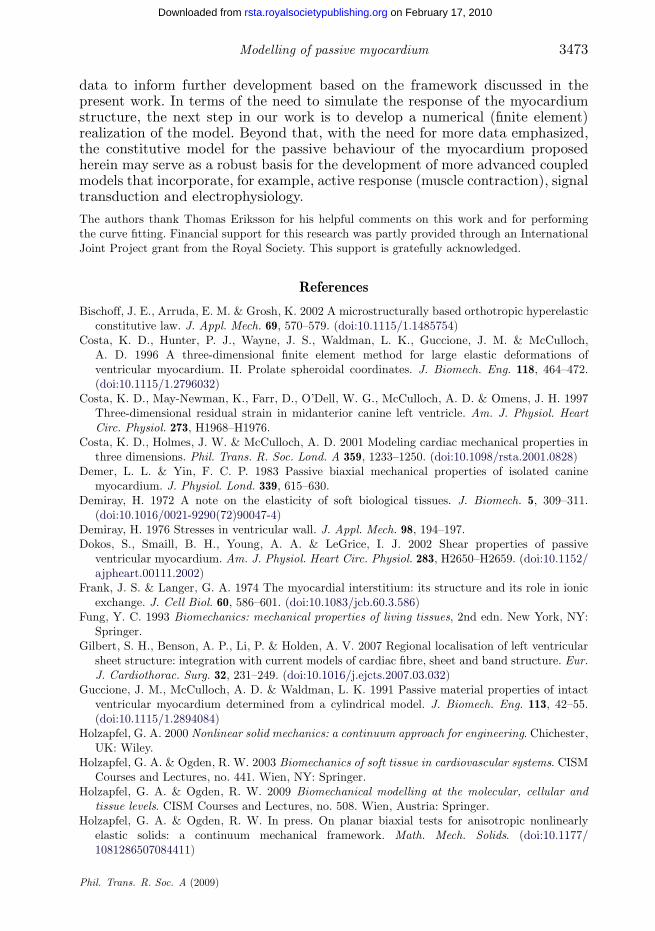
Modelling of passive myocardium 3473
data to inform further development based on the framework discussed in thepresent work. In terms of the need to simulate the response of the myocardiumstructure, the next step in our work is to develop a numerical (finite element)realization of the model. Beyond that, with the need for more data emphasized,the constitutive model for the passive behaviour of the myocardium proposedherein may serve as a robust basis for the development of more advanced coupledmodels that incorporate, for example, active response (muscle contraction), signaltransduction and electrophysiology.
The authors thank Thomas Eriksson for his helpful comments on this work and for performingthe curve fitting. Financial support for this research was partly provided through an InternationalJoint Project grant from the Royal Society. This support is gratefully acknowledged.
References
Bischoff, J. E., Arruda, E. M. & Grosh, K. 2002 A microstructurally based orthotropic hyperelasticconstitutive law. J. Appl. Mech. 69, 570–579. (doi:10.1115/1.1485754)
Costa, K. D., Hunter, P. J., Wayne, J. S., Waldman, L. K., Guccione, J. M. & McCulloch,A. D. 1996 A three-dimensional finite element method for large elastic deformations ofventricular myocardium. II. Prolate spheroidal coordinates. J. Biomech. Eng. 118, 464–472.(doi:10.1115/1.2796032)
Costa, K. D., May-Newman, K., Farr, D., O’Dell, W. G., McCulloch, A. D. & Omens, J. H. 1997Three-dimensional residual strain in midanterior canine left ventricle. Am. J. Physiol. HeartCirc. Physiol. 273, H1968–H1976.
Costa, K. D., Holmes, J. W. & McCulloch, A. D. 2001 Modeling cardiac mechanical properties inthree dimensions. Phil. Trans. R. Soc. Lond. A 359, 1233–1250. (doi:10.1098/rsta.2001.0828)
Demer, L. L. & Yin, F. C. P. 1983 Passive biaxial mechanical properties of isolated caninemyocardium. J. Physiol. Lond. 339, 615–630.
Demiray, H. 1972 A note on the elasticity of soft biological tissues. J. Biomech. 5, 309–311.(doi:10.1016/0021-9290(72)90047-4)
Demiray, H. 1976 Stresses in ventricular wall. J. Appl. Mech. 98, 194–197.Dokos, S., Smaill, B. H., Young, A. A. & LeGrice, I. J. 2002 Shear properties of passive
ventricular myocardium. Am. J. Physiol. Heart Circ. Physiol. 283, H2650–H2659. (doi:10.1152/ajpheart.00111.2002)
Frank, J. S. & Langer, G. A. 1974 The myocardial interstitium: its structure and its role in ionicexchange. J. Cell Biol. 60, 586–601. (doi:10.1083/jcb.60.3.586)
Fung, Y. C. 1993 Biomechanics: mechanical properties of living tissues, 2nd edn. New York, NY:Springer.
Gilbert, S. H., Benson, A. P., Li, P. & Holden, A. V. 2007 Regional localisation of left ventricularsheet structure: integration with current models of cardiac fibre, sheet and band structure. Eur.J. Cardiothorac. Surg. 32, 231–249. (doi:10.1016/j.ejcts.2007.03.032)
Guccione, J. M., McCulloch, A. D. & Waldman, L. K. 1991 Passive material properties of intactventricular myocardium determined from a cylindrical model. J. Biomech. Eng. 113, 42–55.(doi:10.1115/1.2894084)
Holzapfel, G. A. 2000 Nonlinear solid mechanics: a continuum approach for engineering. Chichester,UK: Wiley.
Holzapfel, G. A. & Ogden, R. W. 2003 Biomechanics of soft tissue in cardiovascular systems. CISMCourses and Lectures, no. 441. Wien, NY: Springer.
Holzapfel, G. A. & Ogden, R. W. 2009 Biomechanical modelling at the molecular, cellular andtissue levels. CISM Courses and Lectures, no. 508. Wien, Austria: Springer.
Holzapfel, G. A. & Ogden, R. W. In press. On planar biaxial tests for anisotropic nonlinearlyelastic solids: a continuum mechanical framework. Math. Mech. Solids. (doi:10.1177/1081286507084411)
Phil. Trans. R. Soc. A (2009)
on February 17, 2010rsta.royalsocietypublishing.orgDownloaded from

3474 G. A. Holzapfel and R. W. Ogden
Holzapfel, G. A., Gasser, T. C. & Ogden, R. W. 2000 A new constitutive framework forarterial wall mechanics and a comparative study of material models. J. Elasticity 61, 1–48.(doi:10.1023/A:1010835316564)
Holzapfel, G. A., Gasser, T. C. & Ogden, R. W. 2004 Comparison of a multi-layer structural modelfor arterial walls with a Fung-type model, and issues of material stability. J. Biomech. Eng. 126,264–275. (doi:10.1115/1.1695572)
Horowitz, A., Lanir, Y., Yin, F. C. P., Perl, M., Sheinman, I. & Strumpf, R. K. 1988 Structuralthree-dimensional constitutive law for the passive myocardium. J. Biomech. Eng. 110, 200–207.
Humphrey, J. D. & Yin, F. C. P. 1987 On constitutive relations and finite deformations of passivecardiac tissue. Part I. A pseudo-strain energy function. J. Biomech. Eng. 109, 298–304.
Humphrey, J. D., Strumpf, R. K. & Yin, F. C. P. 1990 Determination of constitutiverelation for passive myocardium. I. A new functional form. J. Biomech. Eng. 112, 333–339.(doi:10.1115/1.2891193)
Hunter, P. J., Nash, M. P. & Sands, G. B. 1997 Computational electromechanics of the heart. InComputational biology of the heart (eds A. V. Panfilov & A. V. Holden), pp. 345–407. Chichester,UK: Wiley.
Huyghe, J. M., van Campen, D. H., Arts, T. & Heethaar, R. M. 1991 The constitutive behaviourof passive heart muscle tissue. A quasi-linear viscoelastic formulation. J. Biomech. 24, 841–849.(doi:10.1016/0021-9290(91)90309-B)
Huyghe, J. M., Arts, T., van Campen, D. H. & Reneman, R. S. 1992 Porous medium finite elementmodel of the beating left ventricle. Am. J. Physiol. Heart Circ. Physiol. 262, H1256–H1267.
Katz, L. N. 1977 Physiology of the heart. New York, NY: Raven Press.Kerckhoffs, R. C. P., Bovendeerd, P. H. M., Kotte, J. C. S., Prinzen, F. W., Smits, K. & Arts, T.
2003 Homogeneity of cardiac contraction despite physiological asynchrony of depolarization: amodel study. Ann. Biomed. Eng. 31, 536–547. (doi:10.1114/1.566447)
LeGrice, I. J., Smaill, B. H., Chai, L. Z., Edgar, S. G., Gavin, J. B. & Hunter, P. J. 1995 Laminarstructure of the heart: ventricular myocyte arrangement and connective tissue architecture inthe dog. Am. J. Physiol. Heart Circ. Physiol. 269, H571–H582.
LeGrice, I. J., Hunter, P. J. & Smaill, B. H. 1997 Laminar structure of the heart: a mathematicalmodel. Am. J. Physiol. Heart Circ. Physiol. 272, H2466–H2476.
MacKenna, D. A., Omens, J. H. & Covell, J. W. 1996 Left ventricular perimysial collagenfibers uncoil rather than stretch during diastolic filling. Basic Res. Cardiol. 91, 111–122.(doi:10.1007/BF00799683)
Merodio, J. & Ogden, R. W. 2002 Material instabilities in fiber-reinforced nonlinearly elastic solidsunder plane deformation. Arch. Mech. 54, 525–552.
Merodio, J. & Ogden, R. W. 2003 Instabilities and loss of ellipticity in fiber-reinforced compressiblenonlinearly elastic solids under plane deformation. Int. J. Solids Structures 40, 4707–4727.(doi:10.1016/S0020-7683(03)00309-3)
Merodio, J. & Ogden, R. W. 2006 The influence of the invariant I8 on the stress–deformation andellipticity characteristics of doubly fiber-reinforced non-linearly elastic solids. Int. J. Non-LinearMech. 41, 556–563. (doi:10.1016/j.ijnonlinmec.2006.02.001)
Nash, M. P. 1998 Mechanics and material properties of the heart using an anatomically accuratemathematical model. PhD thesis, University of Auckland, Auckland, New Zealand.
Novak, V. P., Yin, F. C. P. & Humphrey, J. D. 1994 Regional mechanical properties of passivemyocardium. J. Biomech. Eng. 27, 403–412. (doi:10.1016/0021-9290(94)90016-7)
Ogden, R. W. 1997 Non-linear elastic deformations. New York, NY: Dover Publications.Ogden, R. W. 2003 Nonlinear elasticity, anisotropy and residual stresses in soft tissue. In
Biomechanics of soft tissue in cardiovascular systems (eds G. A. Holzapfel & R. W. Ogden).CISM Courses and Lectures, no. 441, pp. 65–108. Wien, Austria: Springer.
Ogden, R. W. 2009 Anisotropy and nonlinear elasticity in arterial wall mechanics. In Biomechanicalmodelling at the molecular, cellular and tissue levels (eds G. A. Holzapfel & R. W. Ogden). CISMCourses and Lectures, no. 508, pp. 179–258. Wien, Austria: Springer.
Omens, J. H. & Fung, Y. C. 1990 Residual strain in rat left ventricle. Circ. Res. 66, 37–45.Rachev, A. 1997 Theoretical study of the effect of stress-dependent remodeling on arterial geometry
under hypertensive conditions. J. Biomech. 30, 819–827. (doi:10.1016/S0021-9290(97)00032-8)
Phil. Trans. R. Soc. A (2009)
on February 17, 2010rsta.royalsocietypublishing.orgDownloaded from
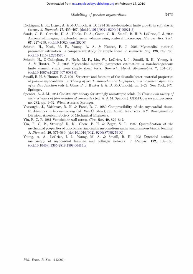
Modelling of passive myocardium 3475
Rodriguez, E. K., Hoger, A. & McCulloch, A. D. 1994 Stress-dependent finite growth in soft elastictissues. J. Biomech. 27, 455–467. (doi:10.1016/0021-9290(94)90021-3)
Sands, G. B., Gerneke, D. A., Hooks, D. A., Green, C. R., Smaill, B. H. & LeGrice, I. J. 2005Automated imaging of extended tissue volumes using confocal microscopy. Microsc. Res. Tech.67, 227–239. (doi:10.1002/jemt.20200)
Schmid, H., Nash, M. P., Young, A. A. & Hunter, P. J. 2006 Myocardial materialparameter estimation—a comparative study for simple shear. J. Biomech. Eng. 128, 742–750.(doi:10.1115/1.2244576)
Schmid, H., O’Callaghan, P., Nash, M. P., Lin, W., LeGrice, I. J., Smaill, B. H., Young, A.A. & Hunter, P. J. 2008 Myocardial material parameter estimation: a non-homogeneousfinite element study from simple shear tests. Biomech. Model. Mechanobiol. 7, 161–173.(doi:10.1007/s10237-007-0083-0)
Smaill, B. H. & Hunter, P. J. 1991 Structure and function of the diastolic heart: material propertiesof passive myocardium. In Theory of heart: biomechanics, biophysics, and nonlinear dynamicsof cardiac function (eds L. Glass, P. J. Hunter & A. D. McCulloch), pp. 1–29. New York, NY:Springer.
Spencer, A. J. M. 1984 Constitutive theory for strongly anisotropic solids. In Continuum theory ofthe mechanics of fibre-reinforced composites (ed. A. J. M. Spencer). CISM Courses and Lectures,no. 282, pp. 1–32. Wien, Austria: Springer.
Vossoughi, J., Vaishnav, R. N. & Patel, D. J. 1980 Compressibility of the myocardial tissue.In Advances in bioengineering (ed. Van C. Mow), pp. 45–48. New York, NY: BioengineeringDivision, American Society of Mechanical Engineers.
Yin, F. C. P. 1981 Ventricular wall stress. Circ. Res. 49, 829–842.Yin, F. C. P., Strumpf, R. K., Chew, P. H. & Zeger, S. L. 1987 Quantification of the
mechanical properties of noncontracting canine myocardium under simultaneous biaxial loading.J. Biomech. 20, 577–589. (doi:10.1016/0021-9290(87)90279-X)
Young, A. A., LeGrice, I. J., Young, M. A. & Smaill, B. H. 1998 Extended confocalmicroscopy of myocardial laminae and collagen network. J Microsc. 192, 139–150.(doi:10.1046/j.1365-2818.1998.00414.x)
Phil. Trans. R. Soc. A (2009)
on February 17, 2010rsta.royalsocietypublishing.orgDownloaded from