Embed Size (px)
Citation preview

Constant Market Shares Analysis:
Uses, Limitations and Prospects
Fredoun Ahmadi-Esfahani
and
Glenn Michael Anderson
Department of Agricultural Economics
The University of Sydney
New South Wales 2006
Australia
Contributed paper presented at the 43rd Annual Conference of the Australian
Agricultural and Resource Economics Society. Held at the Christchurch
Convention Centre and Town Hall (20-22 January 1999). This paper stems from a
project supported by the Rural Industries Research and Development Corporation.

1
Constant Market Shares Analysis:
Uses, Limitations and Prospects
Fredoun Ahmadi-Esfahani and Glenn Michael Anderson
Abstract: Constant market shares (CMS) analysis compares the actual export growth
performance of a country with the performance that would have been achieved if the country had
maintained its exports relative to some standard. The approach was first applied to international
trade in the 1950s and has generally been used to analyse trading patterns and, in particular, the
extent to which poor export performance can be attributed to a loss of ‘competitiveness’. However,
the approach has been open to objections as a tool of description and diagnosis. Recent revisions
appear to meet objections concerning its role as a descriptive tool. However, CMS analysis remains
open to objections as a diagnostic tool owing to the strict theoretical conditions required to yield an
unambiguous interpretation.
In this paper we generalise the constant market share framework based on recent revisions by
Jepma (1986). Alternative models are derived and interpreted with particular attention to the
underlying theoretical conditions required for diagnostic interpretation. We conclude that the
prospects for CMS analysis as a diagnostic tool depend upon further research into its theoretical
foundations, the extent to which the implicit aggregation assumptions can be tested and, of
immediate concern, development of a computer program.
Keywords: CMS analysis, trade, aggregation, Armington model.
Constant market shares analysis (CMS) is a method intended to shed light on the
reasons underlying a country’s comparative export performance. The method requires
a standard for comparison which, depending on the purposes of the analysis, may be
“the world” or a set of similar or closely competitive countries. Further, total exports
are generally disaggregated into categories defined in terms of product-type and
country of destination. The method has generally been used to at least provide an
indication of whether a country’s comparative export performance reflects changing
market shares or global trends in demand. The more ambitious would want the
method to indicate the factors underlying these shifts such as relative prices and
income.
The questions the method is intended to answer include whether a country’s
exports have grown in line with its main competitors (that is, a scale effect) and
whether a country’s comparative performance reflects a strong presence in high-
growth regions or products (product and regional effects, respectively) or competitive
gains in individual markets.
2
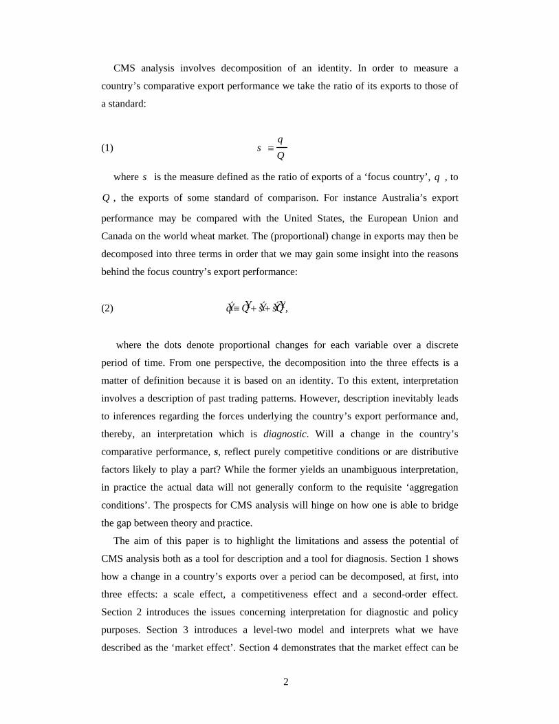
CMS analysis involves decomposition of an identity. In order to measure a
country’s comparative export performance we take the ratio of its exports to those of
a standard:
(1) s q
Q
where s is the measure defined as the ratio of exports of a ‘focus country’, q , to
Q , the exports of some standard of comparison. For instance Australia’s export
performance may be compared with the United States, the European Union and
Canada on the world wheat market. The (proportional) change in exports may then be
decomposed into three terms in order that we may gain some insight into the reasons
behind the focus country’s export performance:
(2) Ý q Ý Q Ý s Ý s ÝQ ,
where the dots denote proportional changes for each variable over a discrete
period of time. From one perspective, the decomposition into the three effects is a
matter of definition because it is based on an identity. To this extent, interpretation
involves a description of past trading patterns. However, description inevitably leads
to inferences regarding the forces underlying the country’s export performance and,
thereby, an interpretation which is diagnostic. Will a change in the country’s
comparative performance, s, reflect purely competitive conditions or are distributive
factors likely to play a part? While the former yields an unambiguous interpretation,
in practice the actual data will not generally conform to the requisite ‘aggregation
conditions’. The prospects for CMS analysis will hinge on how one is able to bridge
the gap between theory and practice.
The aim of this paper is to highlight the limitations and assess the potential of
CMS analysis both as a tool for description and a tool for diagnosis. Section 1 shows
how a change in a country’s exports over a period can be decomposed, at first, into
three effects: a scale effect, a competitiveness effect and a second-order effect.
Section 2 introduces the issues concerning interpretation for diagnostic and policy
purposes. Section 3 introduces a level-two model and interprets what we have
described as the ‘market effect’. Section 4 demonstrates that the market effect can be

3
further decomposed into product and regional effects as well as an interaction effect.
Based on Jepma (1986), the model is a revision the traditional model and overcomes a
major hurdle for descriptive analysis: the order-problem. Section 5 assesses the extent
to which CMS analysis is a viable method for exploratory analysis and how it can be
used to complement other methods such as regression analysis. Appendix A outlines
the theoretical model used in this paper for diagnostic purposes, while Appendix B
describes an alternative procedure for avoiding the order-problem. We conclude that
to fulfil its original promise as a diagnostic tool, CMS analysis requires efficient
empirical tests for consistent aggregation, further research into the theoretical
foundations and, of immediate concern, its own computer package to reduce
computation costs.
1 Basic Model
CMS analysis is a technique for describing trading patterns and trends for the
purpose of policy formulation1. The traditional model was first applied to the study of
international trade by Tyszynski (1951) but has been subject to a number of criticisms
regarding its use as a descriptive tool (Richardson 1971a,b). Jepma (1986) developed
a revised approach which overcomes the most serious of these problems: the ‘order
problem’ (see Section 4.1). Applications of Jepma’s revised model include Jepma
(1986, 1988) and Hoen and Wagener (1989). Ahmadi-Esfahani (1993, 1995) and
Ahmadi-Esfahani and Jensen (1994) use Jepma’s model to analyse Australian wheat
exports to Egypt, Japan and China, respectively. Drysdale and Lu (1996) use the
traditional model to assess Australia’s overall export performance over the decade to
1994. Brownie and Dalziel use the traditional model to analyse New Zealand’s export
performance over the period 1970 to 1984. A comprehensive list of previous
applications and appraisals can be found in Merkies and van der Meer (1988).
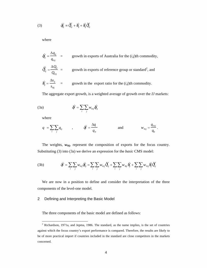
The model presented above, (2), can be thought of as the aggregate version of (3)
below. That is, when exports are differentiated in terms of product type (i=1,…J) and
regional destination (j = 1,…J), the export growth for the focus country in market ij
can be written as follows:
1 For an introduction to the traditional model see Richardson 1971b or Leamer and Stern chapter 7.
4
(3) Ý q ij Ý Q ij Ý s ij Ý s ijÝ Q ij
where
Ý q ij qij
q0ij
= growth in exports of Australia for the (i,j)th commodity,
Ý Q ij Qij
Q0ij
= growth in exports of reference group or standard2, and
Ý s ij sij
s0ij
= growth in the export ratio for the (i,j)th commodity.
The aggregate export growth, is a weighted average of growth over the IJ markets:
(3a) Ý q w0ijÝ q ij
j
i
where
q qijj
i , Ý q
q
q0
and w0ij q0ij
q0
.
The weights, w0ij, represent the composition of exports for the focus country.
Substituting (3) into (3a) we derive an expression for the basic CMS model:
(3b) Ý q w0ijÝ q ij
j
i w0ij
Ý Q ijj
i w0ij
Ý s ijj
i w0ij
Ý s ijÝ Q ij
j
i
We are now in a position to define and consider the interpretation of the three
components of the level-one model.
2 Defining and Interpreting the Basic Model
The three components of the basic model are defined as follows:
2 Richardson, 1971a, and Jepma, 1986. The standard, as the name implies, is the set of countries
against which the focus country’s export performance is compared. Therefore, the results are likely to
be of more practical import if countries included in the standard are close competitors in the markets
concerned.

5
Scale effect: SE w0ijÝ Q ij
j
i . The growth in exports that would have taken place
if individual market shares had remained unchanged.
Competitive effect: CE w0ijÝ s ij
j
i The change in exports if only individual
market shares had changed.
Second-order effect: SOE w0ijÝ s ij
Ý Q ijj
i . A term which captures the effect of
changes in both level of standard exports and market share during the period.
The issue of interpretation has always been at the centre of dispute concerning the
usefulness of CMS analysis. As with any statistical tool interpretation depends on
theory and CMS is no exception. Perhaps the reason for CMS attracting greater
attention over the question of interpretation than other methods (such as regression
analysis) is that it is based on an identity and not derived from an explicit theory.
CMS analysis involves a decomposition of terms of an identity and, as a result, the
empirical results can be consistent with any number of underlying theories.
What has been defined as the ‘market-shares norm’ (Junz and Rhomberg, 1965)
allows us to ‘identify’ the underlying class of theoretical models provided certain
assumptions are met. The norm asserts that a country’s export performance, vis-à-vis
some standard, will depend solely on its competitiveness. Following Leamer and
Stern, 1970, the comparative performance of the focus country will depend solely on
relative prices,
(4a) xij
Xij
fpij
Pij
,
where xij
Xij
, is the ratio of exports of focus country to those of the standard and
pij
Pij
the relative price between the two suppliers. Very few attempts have been made to
address the issue of the type of theoretical model entailed by the market shares norm.
Ooms, 1967, demonstrates the consequences of not assuming constant costs with the
implication that the chosen period ought not be too short (Jepma, 1986). Jepma

6
(1986), as well as revising the CMS framework, defines four models under
progressively less restrictive assumptions starting with constant income, constant
relative prices, uniform income elasticities and constant costs. Merkies and van der
Meer (1988) explicitly model the underlying process in terms of a two-stage budget
procedure, along the same lines as Armington (1969). We shall use their model as the
basis of our own interpretation (see below and Appendix A).
In the Armington two-stage procedure, a given amount of import expenditure is
allocated across goods and then across the suppliers of these goods. The expenditure
to be allocated in the second stage is determined at the first stage. Assuming, in
addition, uniform income elasticities of goods within a group, prices of goods outside
the group will only have an effect through an income effect which changes the total,
but not the composition, of a good consumed. In order to demonstrate the potential of
CMS as a diagnostic tool we assume these conditions can be met. Following Merkies
and van der Meer (1988), the scale and competitive effects can be expressed as
follows:
(4b) Scale Effect in market ij:.
SEij Ý Q ij Ý Q j (1 j )(Ý P ij Ý P j )
(4c) Competitive Effect in market ij:
CEij Ý s ij (1 ij )( Ý p ij Ý P ij )
The scale effect in market ij will be a function of the growth in total expenditure,
Qj , and the change in the price of the product i, Pij , relative to all other products of
region j, Pj (a general price index). The parameter, j is the constant elasticity of
substitution of a CES model. Notice that he competitive effect in market ij is a
function of relative prices alone.
While (4) yields an unambiguous interpretation, the stringency of the conditions
means the interpretation will not generally be valid. Three features of (5) will have a
bearing on the interpretation and viability of CMS as a diagnostic tool. Firstly, the
model assumes that demand for exports of the focus country depends on real
7
expenditure of the standard and the price ratio between the competing suppliers. This
implies that consumers utility-maximising procedure can be represented by a two-
stage process and the choice of standard will have an important bearing on whether
the Armington conditions can be met. Further, each product type is an aggregate over
a number of products and each region represents a large number of consumers.
Uniformity of income elasticities and elasticities of substitution (between suppliers of
the same commodity) within regions and product groups is required if the
relationships postulated by Armington at the micro-level are to be translated into the
same relationships between linear aggregates. These issues need to be borne in mind
when interpreting the CMS model for diagnostic purposes.
The question which most concerns the analyst is in which markets are scale and
competitive effects the greatest and whether they are being targeted by the country’s
exporters. In the following sections we show how the framework may be refined
further to provide a more detailed picture for analysis and policy.
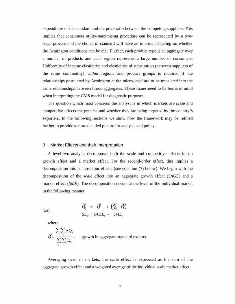
3 Market Effects and their Interpretation
A level-two analysis decomposes both the scale and competitive effects into a
growth effect and a market effect. For the second-order effect, this implies a
decomposition into at most four effects (see equation (7) below). We begin with the
decomposition of the scale effect into an aggregate growth effect (SAGE) and a
market effect (SME). The decomposition occurs at the level of the individual market
in the following manner:
(5a) Ý Q ij Ý Q Ý Q ij Ý Q SEij SAGEij SMEij
where
Ý Q Qij
j
i
Q0ijj
i
, growth in aggregate standard exports.
Averaging over all markets, the scale effect is expressed as the sum of the
aggregate growth effect and a weighted average of the individual scale market effect:

8
(5b) w0ij
Ý Q ijj
j Ý Q wij
Ý Q ij Ý Q j
i
SE SAGE SME
As an aid to interpretation, the scale market effect can be expressed in the
following form:
(5c) SMEkl Ý Q kl Ý Q W0ijÝ Q kl Ý Q ij
j
i k=1,…I.; l= 1,…,J.
where
W0ij Q0ij
Q0ijj
i
.
Equation (5c) is a weighted average of growth differentials between the (k,l)th
market and all markets. A positive scale market effect in the (k,l)th market would
indicate that, on average, growth in this market exceeds growth in other markets. The
market effect would improve the performance of the focus country if its exports are
favourably weighted in this market. Such a weighting would imply a positive market
effect for the focus country.
A market effect for the competitive effect may be defined in a similar fashion.
Firstly, the growth in the export ratio can be expressed as the sum of the growth for
the aggregate (competitive aggregate growth effect, CAGE) and a competitive market
effect (CME):
(6a) Ý s ij Ý s Ý s ij Ý s CEij CAG CMEij
where
s qij
j
i
Qijj
i
export ratio for the aggregate model (2), above.
Averaging over all markets, the competitive effect is expressed as the sum of the
aggregate growth effect and a weighted average of the individual competitive market
effects:

9
(6b) w0ij
Ý s ijj
j Ý s wij
Ý s ij Ý s j
i
CE CAGE CME
Once again, where a market effect does exist, its significance for the focus country
will depend on the weighting the market receives in the country’s total exports. The
competitive market effect therefore indicates the significance of individual
competitive market effects for the focus country’s overall export performance.
Further, as an aid to interpretation, the competitive market effect for the (k,l)th market
can be expressed in the following form:
(6c) CMEkl Ý s kl Ý s w0ijÝ s kl Ý s ij
j
i k=1,…I.; l= 1,…,J.
where (as in (4a), above)
w0ij q0ij
q0ijj
i
.
The competitive market effect in the (k,l)th market is a weighted average of
differentials between the growth in market share in this market and growth in market
share in all other markets.
Finally, the decomposition for the second-order effect is derived by taking the
weighted average of individual effects derived from the product of equations (5a) and
(6a):
(7)
SOE Ý s Ý Q Ý Q wijÝ s ij Ý s
j
i Ý s wij
Ý Q ij Ý Q j
i
wijÝ s ij Ý s Ý Q ij Ý Q
j
i
Interpretation, for descriptive purposes, of the components of the second-order
effect draws upon interpretation of the components of the scale and competitive
effects. For instance, the first component on the right hand side of (7) is the second-
order effect for the aggregate model ((2), above). The second term, considers the
impact of aggregation bias over standard exports (assuming bias is absent from the
export ratios). The third effect indicates the effect of aggregation bias in the export
ratio assuming growth in standard exports are uniform across markets. Finally, the
10
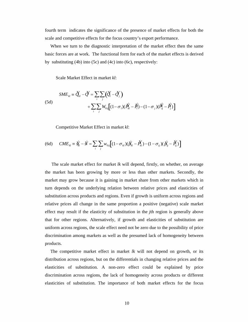
fourth term indicates the significance of the presence of market effects for both the
scale and competitive effects for the focus country’s export performance.
When we turn to the diagnostic interpretation of the market effect then the same
basic forces are at work. The functional form for each of the market effects is derived
by substituting (4b) into (5c) and (4c) into (6c), respectively:
Scale Market Effect in market kl:
(5d)
SMEkl Ý Q kl Ý Q Ý Q l Ý Q j j
i
W0ij (1 l)( Ý P kl Ý P l ) (1 j )( Ý P ij Ý P j ) j
i
Competitive Market Effect in market kl:
(6d) CMEkl Ý s kl Ý s w0ij (1 kl )( Ý p kl Ý P kl ) (1 ij )( Ý p ij Ý P ij ) j
i
The scale market effect for market lk will depend, firstly, on whether, on average
the market has been growing by more or less than other markets. Secondly, the
market may grow because it is gaining in market share from other markets which in
turn depends on the underlying relation between relative prices and elasticities of
substitution across products and regions. Even if growth is uniform across regions and
relative prices all change in the same proportion a positive (negative) scale market
effect may result if the elasticity of substitution in the jth region is generally above
that for other regions. Alternatively, if growth and elasticities of substitution are
uniform across regions, the scale effect need not be zero due to the possibility of price
discrimination among markets as well as the presumed lack of homogeneity between
products.
The competitive market effect in market lk will not depend on growth, or its
distribution across regions, but on the differentials in changing relative prices and the
elasticities of substitution. A non-zero effect could be explained by price
discrimination across regions, the lack of homogeneity across products or different
elasticities of substitution. The importance of both market effects for the focus

11
country will of course depend on the relative importance of each market in the
country’s total exports (through (5b) and (6b)).
In the next section we show that a third level of decomposition is possible. Each
market effect can be decomposed into a regional effect, a product effect and a further
interaction effect. The result is a fully generalised framework for CMS analysis.
4 Two Methods for a Consistent Decomposition of the Markets Effects
A level-three decomposition of the market effect follows on from Jepma’s(1986)
resolution of a problem for descriptive analysis. Following on from a discussion of
the ‘order-problem’, we demonstrate that there are two ways for avoiding the
problem or, in other words, for consistent decomposition of the market effect. The
first approach is based on Jepma’s (1986) work and is referred to as the unconditional
effects model. A second approach also provides a consistent decomposition of the
market effects and is referred to as the conditional effects model (see Appendix B).
Since an interpretation of both models under the market-shares norm would be
repetitive and would not enhance our understanding of the main issues, only the
unconditional effects model is interpreted.
4.1 The ‘order problem’
The order-problem derives its name from the manner in which the scale market
effect is decomposed. Traditionally, in order to be able to discern the extent to which
the market effect could be attributed to a lack of uniformity in growth over products
or regions, the market effect was further decomposed into a regional effect and a
product effect. However, the order in which the decomposition proceeded would
generally lead to different measures for the same (regional or product) effect.
Therefore, CMS analysis was open to the criticism that, even for descriptive purposes,
it was seriously flawed (Richardson 1971a).
The order-problem is illustrated below. The decomposition of the (i,j)th market
effect may take two forms. In the first equation the regional effect, SRE jC , is said to
be decomposed before the product effect, SPEij :
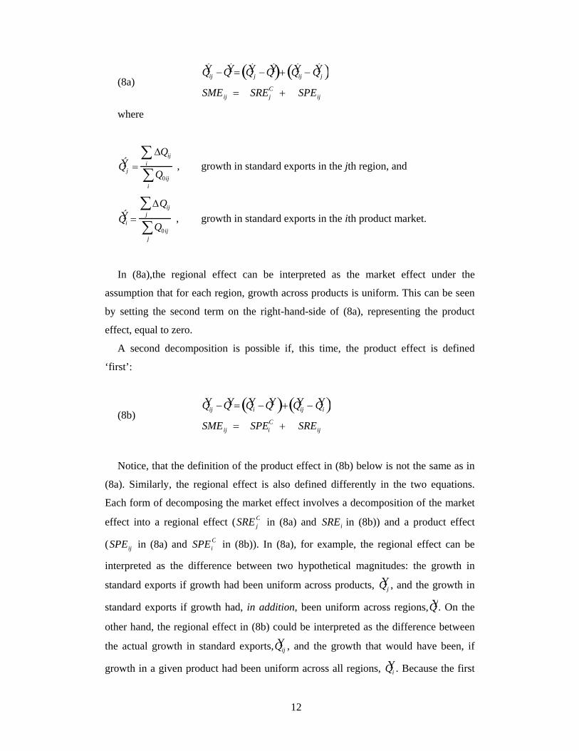
12
(8a) Ý Q ij Ý Q Ý Q j Ý Q Ý Q ij Ý Q j SMEij SREj
C SPEij
where
Ý Q j Qij
i
Q0iji
, growth in standard exports in the jth region, and
Ý Q i Qij
j
Q0ijj
, growth in standard exports in the ith product market.
In (8a),the regional effect can be interpreted as the market effect under the
assumption that for each region, growth across products is uniform. This can be seen
by setting the second term on the right-hand-side of (8a), representing the product
effect, equal to zero.
A second decomposition is possible if, this time, the product effect is defined
‘first’:
(8b) Ý Q ij Ý Q Ý Q i Ý Q Ý Q ij Ý Q i SMEij SPEi
C SREij
Notice, that the definition of the product effect in (8b) below is not the same as in
(8a). Similarly, the regional effect is also defined differently in the two equations.
Each form of decomposing the market effect involves a decomposition of the market
effect into a regional effect (SRE jC in (8a) and SREi in (8b)) and a product effect
(SPEij in (8a) and SPEiC in (8b)). In (8a), for example, the regional effect can be
interpreted as the difference between two hypothetical magnitudes: the growth in
standard exports if growth had been uniform across products, Ý Q j , and the growth in
standard exports if growth had, in addition, been uniform across regions, ÝQ . On the
other hand, the regional effect in (8b) could be interpreted as the difference between
the actual growth in standard exports, Ý Q ij , and the growth that would have been, if
growth in a given product had been uniform across all regions, Ý Q i . Because the first

13
regional effect, SRE jC , of (8a) is defined on the condition that growth is uniform
across products we shall refer to it as the conditional regional effect. The regional
effect of (8b), SPEiC , will be referred to as the unconditional regional effect.
Similarly, the product effect of equation (8b), SPEiC ,will be referred to as the
conditional product effect and the product effect of equation (8a), SPEij , will be
referred to as the unconditional product effect. Appendix B illustrates the relation
between both types of effects in terms of a Venn diagram.
Generally, conditional and unconditional effects will not be the same. For the
traditional model, this has meant that the order in which the market effect was
decomposed could effect the conclusions derived from a CMS model (see
Richardson, 1971b). In the next section we show how Jepma (1986) has resolved the
order-problem and we provide a generalisation of his approach. The model based on
Jepmas’ decomposition is described as an unconditional effects model to distinguish it
from an alternative means for consistently decomposing the market effects (see
Appendix B)3.
4.2 Jepma’s Decomposition and the Unconditional Effects Model
What will be referred to as the unconditional effects model is based on a
decomposition of the market effect suggested by Jepma (1986). Jepma suggested
decomposing the scale market effect into three terms intended to capture the impact of
disparities in growth across regions and products as well as a third term referred to as
the scale interaction effect.
4.2.1 Decomposition of the Scale Market Effect
Based on Jepma (1986), the scale market effect in the (i,j)th market is decomposed
in the following fashion:
3 For a detailed discussion of the order problem and other issues, as well as an extensive
bibliography, see Jepma 1986.

14
(9) Ý Q ij Ý Q Ý Q ij Ý Q i Ý Q ij Ý Q j Ý Q ij Ý Q j Ý Q i Ý Q SMEij SREij + SPEij SIEij
where
SREij = scale regional effect for the (i,j)th market,
SPEij = scale product effect for the (i,j)th market, and
SIEij = scale interaction effect for the (i,j)th market.
A scale regional effect is defined for each product and is the difference between
the actual growth in standard exports and the growth that would have taken place if
product i’s growth had been uniform across regions. An alternative expression
indicates the precise interpretation (for descriptive analysis):
(9a) Ý Q il Ý Q i W0 ji Ý Q il Ý Q ij
j l=1,…J.
where
W0 ji
Q0ij
Q0ijj
.
Equation (9a) is the weighted average of growth differentials between region l and
all regions in terms of product type i. Therefore, a positive (negative) scale regional
effect, Ý Q ij ÝQ i , would indicate that the growth differential between region l and each
of the other regions is, on average, positive (negative) for the ith product market. For
example, if the growth in standard exports of wheat to Japan exceeded those of its
neighbours then this would lead to a positive scale regional effect for wheat in Japan.
The impact on the focus country will depend on the relative weighting of wheat to
Japan in its exports. The scale regional effect for the jth region therefore indicates the
weighted average of the scale regional effects for the focus country:
(9a.1) SRE j w0ijÝ Q ij Ý Q i
i
The total regional effect is the summation of the effect for each region:
15
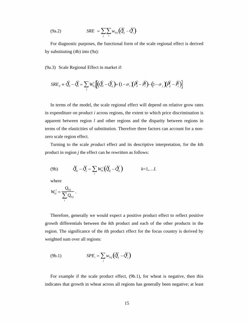
(9a.2) SRE w0iji Ý Q ij Ý Q i
j
For diagnostic purposes, the functional form of the scale regional effect is derived
by substituting (4b) into (9a):
(9a.3) Scale Regional Effect in market il:
SREil Ý Q il Ý Q i W0 ji Ý Q il Ý Q ij 1 l Ý P il Ý P l 1 j Ý P ij Ý P j
j
In terms of the model, the scale regional effect will depend on relative grow rates
in expenditure on product i across regions, the extent to which price discrimination is
apparent between region l and other regions and the disparity between regions in
terms of the elasticities of substitution. Therefore three factors can account for a non-
zero scale region effect.
Turning to the scale product effect and its descriptive interpretation, for the kth
product in region j the effect can be rewritten as follows:
(9b) Ý Q kj Ý Q j W0ij Ý Q kj Ý Q ij
i k=1,…I.
where
W0ij
Q0ij
Q0iji
.
Therefore, generally we would expect a positive product effect to reflect positive
growth differentials between the kth product and each of the other products in the
region. The significance of the ith product effect for the focus country is derived by
weighted sum over all regions:
(9b.1) SPEi w0ijj Ý Q ij Ý Q j
For example if the scale product effect, (9b.1), for wheat is negative, then this
indicates that growth in wheat across all regions has generally been negative; at least

16
in those markets regions which are of importance to wheat exporters of the focus
country. Aggregating over the scale product effects, we derived the total scale
product effect:
(9b.2) SPE w0ijj Ý Q ij Ý Q j
i
For example, if the total scale product effect is positive, despite a negative effect
for wheat, then this indicates a weighting in favour other products, such as beef, with
positive scale product effects.
Interpretation of the scale product effect for diagnostic purposes is straight-forward
under the assumed model. From (4b), we derive the following:
(9b.3) Scale Product Effect in market kj:
SPEkj Ý Q kj Ý Q j (1 j )(Pkj Ý P j )
Under the model, the scale product effect for each product in region l reflects
changes in the relative price of the product. Unless the product is highly
differentiated, a fall in relative prices will yield a positive scale product effect.
Finally, the scale interaction effect is interpreted as the combined effect of non-
uniformity of growth across regions and product types. To interpret the scale
interaction effect for descriptive purposes, it is best rewritten as follows:
(9c.1) SIEij SMEij Ý Q j Ý Q Ý Q i Ý Q
The last two terms were defined in the previous section as the conditional regional
effect, SRE jC , and conditional product effect,SPEi
C (see Section 4.1, above, or
Appendix B). Whereas the unconditional scale regional effect, SREij , makes no
assumption regarding the uniformity, or otherwise, of growth across products, the
corresponding conditional effect, SRE jC , assumes that growth for regions in aggregate
is an unbiased measure of growth for each region. In other words if growth across
products were assumed uniform, then the market effect in the (i,j)th market would be
17
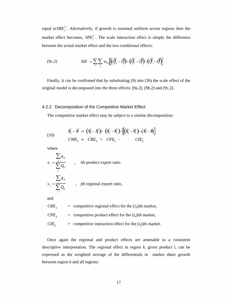
equal toSRE jC . Alternatively, if growth is assumed uniform across regions then the
market effect becomes, SPEiC . The scale interaction effect is simply the difference
between the actual market effect and the two conditional effects:
(9c.2) SIE w0ijÝ Q ij Ý Q Ý Q j Ý Q Ý Q i Ý Q
j
i
Finally, it can be confirmed that by substituting (9) into (3b) the scale effect of the
original model is decomposed into the three effects: (9a.2), (9b.2) and (9c.2).
4.2.2 Decomposition of the Competitive Market Effect
The competitive market effect may be subject to a similar decomposition:
(10) Ý s ij Ý s Ý s ij Ý s i Ý s ij Ý s j Ý s ij Ý s j Ý s i Ý s CMEij CREij + CPEij CIEij
where
si qij
j
Qijj
, ith product export ratio.
s j qij
i
Qiji
, jth regional export ratio,
and
CREij = competitive regional effect for the (i,j)th market,
CPEij = competitive product effect for the (i,j)th market,
CIEij = competitive interaction effect for the (i,j)th market.
Once again the regional and product effects are amenable to a consistent
descriptive interpretation. The regional effect in region k, given product i, can be
expressed as the weighted average of the differentials in market share growth
between region k and all regions:
18
(10a) Ý s ik Ý s i w0 ji Ý s ik Ý s ij
j
where
w0 ji
q0ij
q0ijj
4.
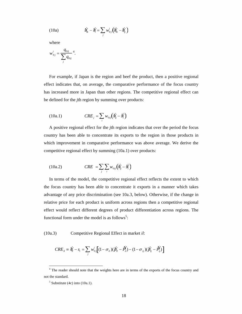
For example, if Japan is the region and beef the product, then a positive regional
effect indicates that, on average, the comparative performance of the focus country
has increased more in Japan than other regions. The competitive regional effect can
be defined for the jth region by summing over products:
(10a.1) CRE j w0ijÝ s ij Ý s i
i
A positive regional effect for the jth region indicates that over the period the focus
country has been able to concentrate its exports to the region in those products in
which improvement in comparative performance was above average. We derive the
competitive regional effect by summing (10a.1) over products:
(10a.2) CRE w0iji Ý s ij Ý s i
j
In terms of the model, the competitive regional effect reflects the extent to which
the focus country has been able to concentrate it exports in a manner which takes
advantage of any price discrimination (see 10a.3, below). Otherwise, if the change in
relative price for each product is uniform across regions then a competitive regional
effect would reflect different degrees of product differentiation across regions. The
functional form under the model is as follows5:
(10a.3) Competitive Regional Effect in market il:
CREil Ý s il si w0 ji (1 il )( Ý p il Ý P il) (1 ij )( Ý p ij Ý P ij)
j
4 The reader should note that the weights here are in terms of the exports of the focus country and
not the standard. 5 Substitute (4c) into (10a.1).
19
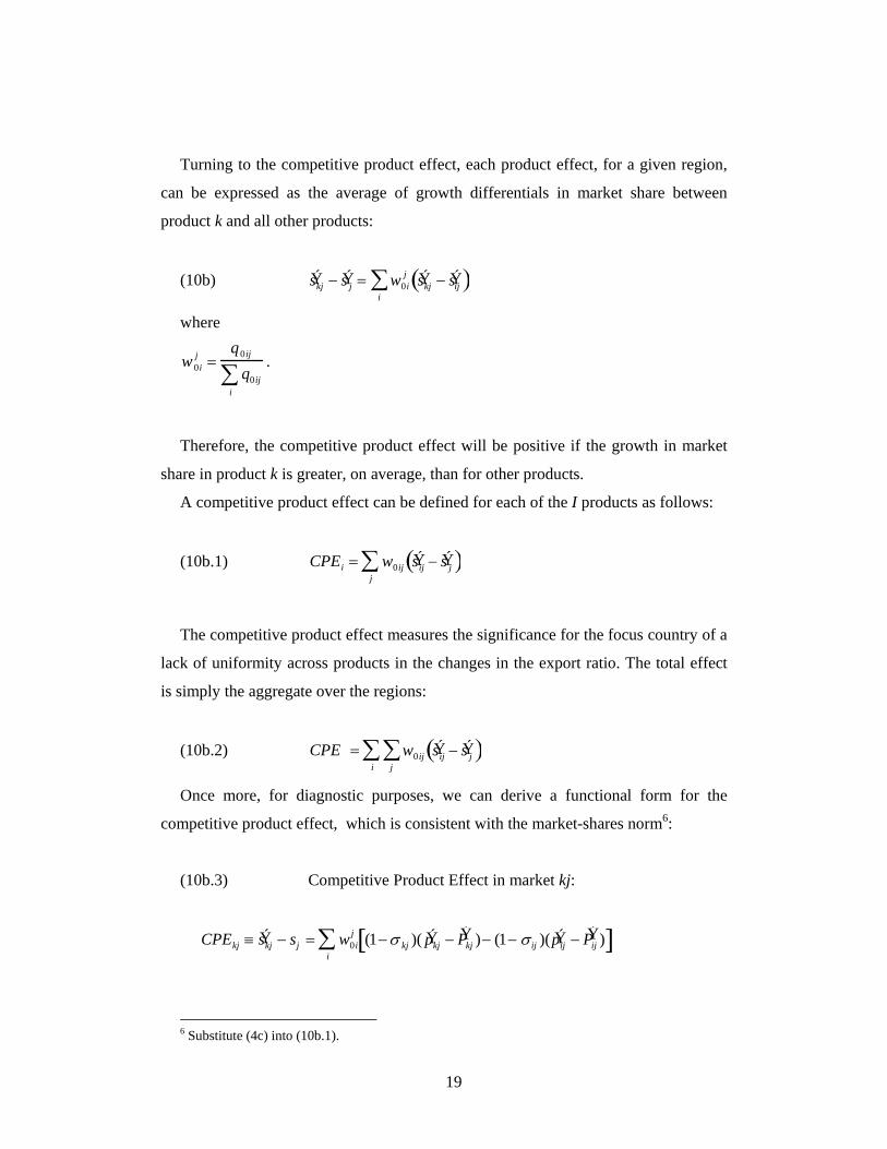
Turning to the competitive product effect, each product effect, for a given region,
can be expressed as the average of growth differentials in market share between
product k and all other products:
(10b) Ý s kj Ý s j w0ij Ý s kj Ý s ij
i
where
w0ij
q0ij
q0iji
.
Therefore, the competitive product effect will be positive if the growth in market
share in product k is greater, on average, than for other products.
A competitive product effect can be defined for each of the I products as follows:
(10b.1) CPEi w0ijj Ý s ij Ý s j
The competitive product effect measures the significance for the focus country of a
lack of uniformity across products in the changes in the export ratio. The total effect
is simply the aggregate over the regions:
(10b.2) CPE w0ijj Ý s ij Ý s j
i
Once more, for diagnostic purposes, we can derive a functional form for the
competitive product effect, which is consistent with the market-shares norm6:
(10b.3) Competitive Product Effect in market kj:
CPEkj Ý s kj sj w0ij (1 kj )( Ý p kj Ý P kj ) (1 ij )( Ý p ij Ý P ij )
i
6 Substitute (4c) into (10b.1).
20
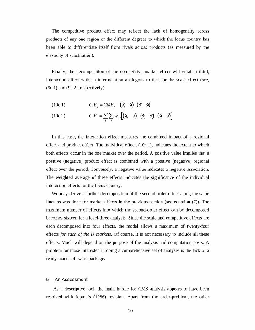
The competitive product effect may reflect the lack of homogeneity across
products of any one region or the different degrees to which the focus country has
been able to differentiate itself from rivals across products (as measured by the
elasticity of substitution).
Finally, the decomposition of the competitive market effect will entail a third,
interaction effect with an interpretation analogous to that for the scale effect (see,
(9c.1) and (9c.2), respectively):
(10c.1) CIEij CMEij Ý s j Ý s Ý s i Ý s
(10c.2) CIE w0ijÝ s ij Ý s Ý s j Ý s Ý s i Ý s
j
i
In this case, the interaction effect measures the combined impact of a regional
effect and product effect The individual effect, (10c.1), indicates the extent to which
both effects occur in the one market over the period. A positive value implies that a
positive (negative) product effect is combined with a positive (negative) regional
effect over the period. Conversely, a negative value indicates a negative association.
The weighted average of these effects indicates the significance of the individual
interaction effects for the focus country.
We may derive a further decomposition of the second-order effect along the same
lines as was done for market effects in the previous section (see equation (7)). The
maximum number of effects into which the second-order effect can be decomposed
becomes sixteen for a level-three analysis. Since the scale and competitive effects are
each decomposed into four effects, the model allows a maximum of twenty-four
effects for each of the IJ markets. Of course, it is not necessary to include all these
effects. Much will depend on the purpose of the analysis and computation costs. A
problem for those interested in doing a comprehensive set of analyses is the lack of a
ready-made soft-ware package.
5 An Assessment
As a descriptive tool, the main hurdle for CMS analysis appears to have been
resolved with Jepma’s (1986) revision. Apart from the order-problem, the other

21
problem cited in the literature has been what Richardson (1971a,b) has called the
index-problem: the choice of an appropriate base year. Jepma (1986) has suggested a
method of shifting weights (that is, the w’s) to allow for changes in export
composition over time. In our own empirical analysis, we have calculated the CMS
model on an annual basis and taken the average over a period or four or five years,
with due account for any outlying years.
On the other hand, the issue of diagnostic interpretation remains open with few
attempts to explore the theoretical foundations of the CMS model. We saw that an
unambiguous interpretation requires the market-shares norm, which assumes that
market shares depend only on the prices of competing suppliers within a market. The
market-shares norm places CMS analysis squarely within the same class as the
Armington models and shares in its flaws as well as its benefits.
The benefits include the relative simplicity of diagnostic interpretation. However,
as we have seen, further analysis would be required to determine, for instance,
whether competitive effects were due to price or non-price factors. The advantage of
CMS analysis is that it is able to yield quite precise hypotheses and thereby indicate
the direction for further research using other quantitative, as well as qualitative,
methods. The potential drawback is the inapplicability of the strong separability
assumptions required by the model (for a critical study, see Alston, Carter and Pick
1990). In fact, the issue is really one of being able to measure any bias that the model
may render to the ‘true’ interpretation. An explicit model, such as the one used in this
paper, at least yields a set of refutable maintained hypotheses, such as the presumed
two-stage budgeting process.
Another set of issues revolve around the applicability of the three aggregation
conditions: the definition of regions, products and the standard. Is it appropriate, for
example, to treat East Asia, or even Japan, as one region, or should they be
disaggregated? The answer will depend on the similarity of consumers within regions
and the absence of distribution effects. For instance, we need to be sure the manner in
which growth is distributed across consumers within any one region will not affect
market shares. Further, the relative prices of goods within a product category would
need to be reasonably fixed to assure the analyst that distributional factors did not
influence product shares. The choice of standard may also be classed as an
aggregation problem. To what extent will the choice of countries to be included or

22
excluded from the standard affect the results? Much work needs to be done to clarify
the issues underlying the diagnostic interpretation of the CMS model.
Through-out the analysis, we have assumed quantities to be demand-determined.
Assuming constant costs allows us to take relative prices as determined by the cost-
conditions in the supplying region in which case a change in relative prices can be
unambiguously associated with differential wage, productivity or technological
growth. The supply conditions, at least, limits analysis to changes over the medium to
long run, while demand conditions may place an upper limit on the length of the
period (due to changing tastes).
Concerning the prospects for further research, given the stringent conditions
underlying the market-shares norm, it is not surprising that the CMS framework has
come under attack for lacking an unambiguous interpretation (Houston, 1967; Ooms,
1967). The most important issue appears to be selecting an appropriate level of
disaggregation by region and product type. One the other hand, the CMS model may
itself yield such criteria.(Leamer and Stern, 1971). For instance, a reasonably straight-
forward algorithm for choosing the level of disaggregation may be as follows: select
the level of disaggregation for which marginal increase in the product (regional)
effect from disaggregation of products (regions) was zero. Unfortunately, there may
be no reason to expect such a relationship even if the data were available. Houston
(1968), for example, found that there was no monotonic relation between the level of
disaggregation and the structural effects to be found in his data.
Clustering methods may be another way of tackling the problem of aggregating
over products and consumers. Pudney (1981) applies cluster analysis to the task of
grouping goods according to their estimated elasticities of substitution. The work of
Alston, Carter, Green and Pick (1990) points the way to apparently more generalised
investigation of the structure of consumer preferences. The tests involve non-
parametric analysis of consumption patterns to determine whether they are consistent
with the axioms of revealed preference and, in particular, the implications of
homothetic preferences. Further, testing for cointegration among prices to ascertain
whether any two products can be grouped promises to provide a more reliable and
efficient method for dealing with the problem of product aggregation.
Although we have only touched on what appear to be the main outstanding issues,
it is apparent that there is much scope for further theoretical and applied research.
However, there remains a practical hurdle. The analyst needs to be able to enter a

23
large amount of data and produce a number of models differing in terms of the level
of disaggregation and decomposition. In order to pay due attention to the issues raised
above, and combine CMS analysis with other statical tools such as regression
analysis, CMS analysis requires its own software package. Otherwise the prospect for
CMS analysis is severely limited.
6 Conclusions
In this paper we have shown that the CMS model, based on Jepma’s revised
framework, can be generalised and extended to exploit to the full its descriptive and
diagnostic potential. An important contribution of this paper has been to provide a
general framework for descriptive analysis. Further, we have highlighted the potential
role for CMS in suggesting hypotheses and complementing other methods of
quantitative analysis.
For descriptive analysis, the CMS framework enables a progressively more
detailed examination of trading patterns. Starting with a level-one analysis, the analyst
can gain an idea of the relative importance of scale, competitive and second-order
effect for the country’s export performance. A level-two analysis indicates the relative
importance of growth or market effects. Further, if a market effect appears significant,
it can be decomposed into regional and product effects as part of a level-three
analysis.
While Jepma’s revised framework places descriptive analysis on surer
foundations, diagnosis and policy analysis will remain open to dispute. We have
demonstrated how the various scale and competitive effects may be interpreted under
the market-shares norm using Armington’s suggestion for modelling products
differentiated by country of origin. The interpretation of CMS in terms of the market-
shares norm generates a set of well-defined hypotheses given the assumptions
underlying the market-shares norm. For instance, CMS may tell us that there has been
a significant competitive effect over a period, but it will not indicate the extent to
which price or non-price competition is responsible. Therefore, there is scope for
further applied work in testing the hypotheses generated through CMS analysis, as
well as testing the extent to which the market-shares norm is applicable to the data on
hand.
CMS analysis will generate hypotheses which are refutable, if the model used for
diagnostic interpretation is explicitly specified. In this way, the maintained

24
hypotheses of the market-shares norm, as well as those suggested by CMS analysis,
can be tested. However, without a standard computer package, the costs of CMS will
limit applied research and, as a likely consequence, also limit research into its
theoretical foundations. For these reasons the potential for CMS analysis, particularly
as a tool for diagnosis, has yet to be fully explored and exploited.
References:
Ahmadi-Esfahani F.Z. 1993, ‘An analysis of Egyptian wheat exports: a constant
market shares approach’, Oxford Agrarian Studies, Vol. 21, pp31-39.
Ahmadi-Esfahani F.Z. and Jenson, P.H. 1994, ‘Impact of the US-EC price war on
major wheat exporters’ shares of the Chinese market’ Agricultural Economics,
Vol. 10, pp61-70.
Ahmadi-Esfahani F.Z. 1995, ‘Wheat market shares in the presence of Japanese import
quotas’ Journal of Policy Modeling, Vol. 17, pp315-23.
Alston, J.M., Carter, C.A, Green, R. and Pick, D. 1990, ‘Whither Armington trade
models’, American Journal of Agricultural Economics, pp455-467.
Armington, 1969, ‘A theory of demand for products distinguished by place and
production’, IMF Staff Papers, 16, pp159-76.
Brownie, S. Dalziel, P. 1993, ‘Shift-Share Analyses of New Zealand Exports, 1970-
1984’ New Zealand Economic Papers, Vol. 27, pp233-49.
Drysdale, P. and Lu, W. 1996, Australia’s Export Performance in East Asia, Pacific
Economic Paper, No. 259, Australia-Japanese Research Centre.
Green, H.A.J. 1964, Aggregation in Economic Analysis, Princeton, N.J: Princeton
University Press.
Hoen, H.W. and Wagener, H.-J. 1989, ‘Hungary’s exports to the OECD: A CMS
analysis’ Acta Oeconomica, Vol. 40, pp65-77.
Houston, D.B. 1967, ‘The shift and share analysis of regional growth: a critique’
Southern Economic Journal, Vol. 33, pp577-81.
Jepma, C.J. 1986, Extensions and Application Possibilities of the Constant-Market-
Shares Analysis, Rijkusuniversiteit, Groningen.
Jepma, C.J. 1988 ‘Extensions of the Constant-Market-Shares analysis with an
application to long-term export data of developing countries’, in J.G.
Williamson and V.R. Panchamukhi 1988-89, The Balance between Industry
and Agriculture in Economic development, Vol. 2: Sector Porportions:
25
proceedings of the Eighth World Congress of the International Economic
Association, Delhi, India. New York : St. Martin's Press.
Junz, H.B. and Rhomberg, R.R. 1965, ‘Prices and Export Performance of Industrial
Countries, 1953-63’, IMF Staff Papers, pp224-269.
Leamer, E.E. and Stern, R.M. 1970, Quantitative International Economics, Boston:
Allen & Bacon.
Merkies, A.H.Q.M. and van der Meer, T. 1988, ‘A theoretical foundation for CMS
analysis’ Empirical Economics, Vol. 13, pp65-80.
Ooms, V.D. 1967, ‘Models of comparative export performance’ Yale Economic
essays,7, pp103-41.Pudney, S.E. 1981, ‘An empirical method of
approximating the separable structure of consumer preferences’ Review of
Economic Studies, pp561-577.
Richardson, J.D. 1971a, ‘Constant-market-shares analysis of export growth’ Journal
of International Economics, Vol. 1. pp227-39.
Richardson, J.D. 1971b, ‘Some sensitivity tests for a “constant-market-shares”
analysis of export growth’ Review of Economics and Statistics, LIII, pp300-4.
Tyszynski, H. 1951, ‘World Trade in manufactured commodities, 1899-1950’ The
Manchester School of Economic and Social Studies Vol. 19, pp272-304.

26
Appendix A
Interpretation of Unconditional Model under the CES Armington
Model
(Based on a model derived in Merkies and van der Meer,1988)
Interpretation of Level One Model
Scale Effect in market ij:
SEij Ý Q ij Ý Q j (1 j )(Ý P ij Ý P j )
Competitive Effect in market ij:
CEij Ý s ij (1 ij )( Ý p ij Ý P ij )
Interpretation of Level Two Model
Scale Market Effect in market kl:
SMEkl Ý Q kl Ý Q W0ijÝ Q l Ý Q j (1 l)(
Ý P kl Ý P l ) (1 j )(Ý P ij Ý P j )
j
i
Competitive Market Effect in market kl:
CMEkl Ý s kl Ý s w0ij (1 kl )( Ý p kl Ý P kl ) (1 ij )( Ý p ij Ý P ij ) j
i
Interpretation of Level Three Model
Scale Regional Effect in market il:
SREil Ý Q il Ý Q i W0 ji Ý Q il Ý Q ij
j W0 j
i Ý Q il Ý Q ij 1 l Ý P il Ý P l 1 j Ý P ij Ý P j j
Scale Product Effect in market kj:
SPEkj Ý Q kj Ý Q j (1 j )(Pkj Ý P j )

27
Competitive Regional Effect in market ik:
CREil Ý s il Ý s i w0 ji (1 il )( Ý p il Ý P il) (1 ij )( Ý p ij Ý P ij)
j
Competitive Product Effect in market kj:
CPEkj Ý s kj Ý s j w0ij (1 kj )( Ý p kj Ý P kj ) (1 ij )( Ý p ij Ý P ij )
i
Appendix B
The Conditional Effects Model
The decomposition suggested by Jepma (1986) was based on the unconditional
regional and product effects. An alternative model, which also decomposes the market
effect consistently, will be introduced in this appendix. In the conditional effect
model, the market effects are decomposed into conditional product and regional
effects as well as an interaction term. However, the interaction effects defined in the
previous section are common for both models.
The scale and competitive effects for each market are defined in (B.1) and (B.2)
below. Since the complete model is derived in the same manner as for the
unconditional effects we will not repeat the steps here.
Decomposition of the scale market effect:
(B.1) Ý Q ij Ý Q Ý Q j Ý Q Ý Q i Ý Q Ý Q ij Ý Q Ý Q j Ý Q Ý Q i Ý Q MEij SRE j
C SPEiC SIEij
Decomposition of the competitive market effect:
(B.2) Ý s ij Ý s Ý s ij Ý s i Ý s ij Ý s j Ý s i Ý s Ý s ij Ý s j CME CRE j
C CPEiC CIE
where

28
CRE jC = conditional competitive regional effect for the (i,j)th market,
CPEiC = conditional competitive product effect for the (i,j)th market, and
CIEij = competitive interaction effect for the (i,j)th market.
Unlike its counterpart in the unconditional effects model, the conditional regional
effect for the scale (competitive) effect assumes standard exports (export ratios) grow
uniformly across products and measures the extent of aggregation bias across regions.
Similarly the conditional product effect for the scale (competitive) effect assumes that
standard exports (export ratios) grow uniformly across regions and measures the
extent of aggregation bias across products.
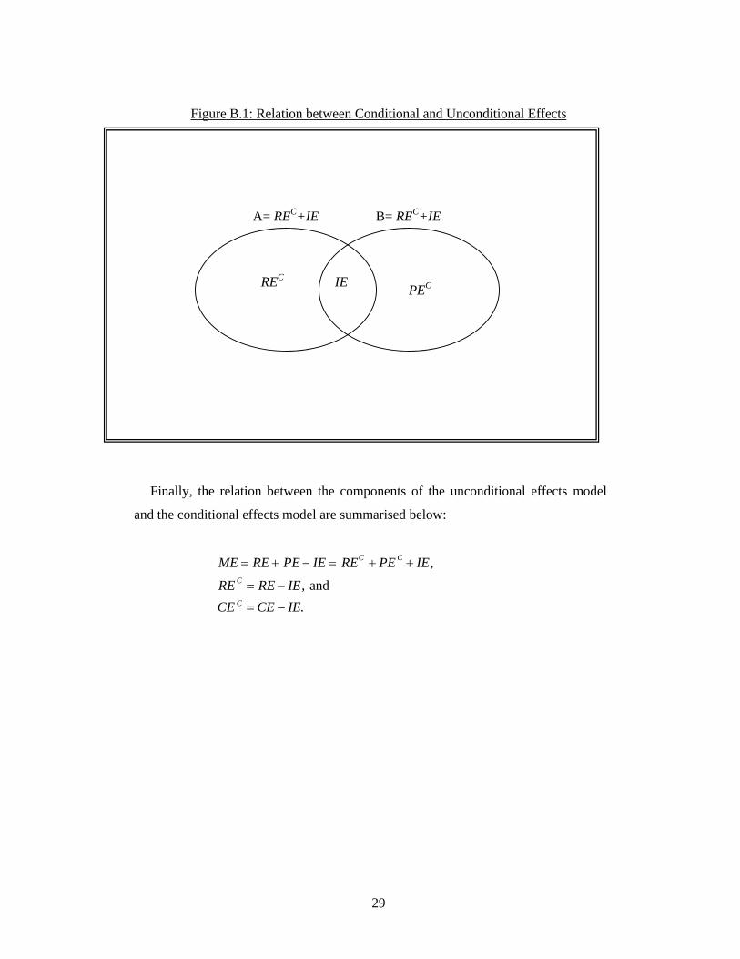
It is beyond the scope of this paper to attempt any clear judgement as to which of
the two models one ought to choose. The relation between the conditional and
unconditional effects may be represented through a Venn diagram (Fig. B.1). In the
Venn diagram below, the area of each circle, A and B, respectively represents the
regional and product effects. Their union represents the market effect and the
intersection of the two circles represents the interaction effect.
The conditional regional effect is derived under the assumption that, for each
region, growth is uniform across products. This is equivalent to assuming that the
(unconditional) product effect is zero which excludes the whole area B. The
remainder of the area (A+B complement B), represents the conditional regional effect.
In addition, the diagram demonstrates that it is possible for the interaction effect to
be zero while the regional and product effects are non-zero. This would be the case if
some markets experienced one effect or the other, but not both. In this case, the
conditional and unconditional effect would be the same.
29
Figure B.1: Relation between Conditional and Unconditional Effects
Finally, the relation between the components of the unconditional effects model
and the conditional effects model are summarised below:
ME RE PE IE REC PE C IE,
RE C RE IE, and
CE C CE IE.
A= REC+IE
PECREC IE
B= REC+IE