Consistent and complete data and “expert” mining in medicine

Boris Kovalerchuk1, Evgenii Vityaev2. James F. Ruiz3 1Department of Computer Science, Central Washington University, Ellensburg, WA, 98926-7520, USA, borisk@tahoma.cwu.edu 2Institute of Mathematics, Russian Academy of Sciences, Novosibirsk 630090, Russia vityaev@math.nsc.ru 3Department of Radiology, Woman’s Hospital, Baton Rouge, LA 70895-9009, USA, MDJR@womans.com

The ultimate purpose of many medical data mining systems is to create formalized knowledge for a computer-aided diagnostic system, which can in turn, provide a second diagnostic opinion. Such systems should be consistent and complete as much as possible. The system is consistent if it is free of contradictions (between rules in a computer-aided diagnostic system, rules used by an experienced medical expert and a database of pathologically confirmed cases). The system is complete if it is able to cover (classify) all (or largest possible number of) combinations of the used attributes. A method for discovering a consistent and complete set of diagnostic rules is presented in this chapter. Advantages of the method are shown for development of a breast cancer computer-aided diagnostic system

1 Introduction

Stages. Knowledge discovery is a complex multistage process. These stages include initial understanding the problem domain, understanding and preparation of data. Data mining, evaluation, and use of discovered knowledge follow the first three stages. In this chapter, knowledge discovery stages for two methods (BEM and MMDR)are presented. These methods belong to the promising class of complete and consistent data mining methods. Such methods produce consistent knowledge, i.e., knowledge free of contradictions (between rules in a computer-aided diagnostic system, rules used by an experienced medical expert and a database of pathologically confirmed cases). Similarly complete methods

produce complete knowledge systems (models), i.e., models which classify all (or largest possible number of) combinations of the used attributes.

Data mining paradigms. Several modern approaches for knowledge discovery are known in the medical field. Neural networks, nearest neighbor methods, discriminant analysis, cluster analysis, linear programming, and genetic algorithms are among the most common knowledge discovery tools used in medicine.

These approaches are associated with different learning paradigms, which involve four major components:

− Representation of background and associated knowledge,

− Learning mechanism,

− Representation of learned knowledge, and

− Forecast performer.

Representation of background and associated knowledge sets a framework for representing prior knowledge. A learning mechanism produces new (learned) knowledge and identifies parameters for the forecast performer using prior knowledge. Representation of learned knowledge sets a framework for use of this knowledge including forecast and diagnosis. A forecast performer serves as a final product, generating a forecast from learned knowledge.

Figure 1 shows the interaction of these components of a learning paradigm. The training data and other available knowledge are embedded into some form of knowledge representation. The learning mechanism (method/algorithm) uses available information to produce a forecast performer and possibly a separate entity, learned knowledge, which can be communicated to medical experts.

The most controversial problem is the relation between a forecast performer and learned knowledge. The learned knowledge can exist in different forms. The widely accepted position is that the learning mechanism of a data mining system produces knowledge only if that knowledge can be put in a human-understandable form (Fu, 1999).

Some DM paradigms (such as neural networks) do not generate learned knowledge as a separate human-understandable entity. A forecast performer (trained neural network) contains this knowledge implicitly, but cryptically, coded as a large number of weights.

This knowledge should be decoded and communicated into the terms of the problem to be solved. Fu (1999) noted “Lack of comprehension causes concern about the credibility of the result when neural networks are applied to risky domains, such as patient care”. As noted in many recent

publications, obtaining comprehensible learned knowledge is one of the important and promising directions in data mining (e.g. (Muggleton, 1999; Graven and Shavlik, 1997)).

Learning mechanism

Prior knowledge representation

Learned knowledge

Forecastperformer

Resulting blockLearning block

Training data

Figure 1. Learning paradigm

This consideration shows the importance of knowledge representation to obtain decodable understandable knowledge and a understandable forecast performer. Five major forms of knowledge representation are listed below (Langley and Simon, 1995):

1. A multilayer network of units (neural network paradigm).

2. Specific cases applied to new situations by matching with new cases (instance-based learning paradigm).

3. Binary features used as the conditions and actions of rules (genetic algorithms paradigm).

4. Decision trees and propositional If-Then rules (rule induction paradigm).

5. Rules in first-order logic form (Horn clauses as in the Prolog language) (analytic learning paradigm).

6. A mixture of the previous representations (hybrid paradigm).

As it was already discussed, neural network learning identifies the forecast performer, but does not produce knowledge in a form understandable by humans.. The rule induction and analytical learning paradigms produce

learned knowledge in the form of understandable if-then rules and the forecast performer is a derivative of these forms of knowledge. Therefore, this chapter concentrates on rule induction and analytical learning paradigms.

The next important component of each of leaning paradigms is a learning mechanism. These mechanisms include specific and general formal and informal steps. These steps are challenging for many reasons. Currently, the least formalized steps are reformulating the actual problem as a learning problem and identifying an effective knowledge representation.

It has become increasingly evident that effective knowledge representation is an important problem for the success of data mining. Close inspection of successful projects suggests that much of the power comes not from the specific induction method, but from proper formulation of the problems and from crafting the representation to make learning tractable (Langley and Simon, 1995). Thus, the conceptual challenges in data mining are:

− proper formulation of the problems and

− crafting the knowledge representation to make learning meaningful and tractable.

Munakata (1999) and Mitchell (1999) point out several especially promising and challenging tasks in current data mining:

1.enhancement of background and associated knowledge using

- incorporation of more comprehensible, non-oversimplified, real-world types of data,

- human-computer interaction for extracting background knowledge,

2. enhancement of learning mechanism using

-interactive human guided data mining and

-optimization of decisions, rather than prediction.

3. hybrid systems for taking advantage of different methods of data mining.

4. Learning from multiple databases and Web based systems.

Traditionally, the knowledge representation process in medical diagnosis includes two major steps:

extracting about a dozen diagnostic features from data or images and

representing a few hundred data units using the extracted features.

Data mining in fields outside of medicine tend to use larger databases and discover larger sets of rules using these techniques. However, mammography archives at hospitals around the world contain millions of mammograms and biopsy results. Currently, the American College of Radiology (ACR) supports the National Mammography Database (NMD) Project (http://www.eskimo.com/~briteoo/nmd) with a unified set of features (BI-RADS, 1998).

Several universities and hospitals have developed mammography image bases that are available on the Internet. Such efforts provide the opportunity for large-scale data mining and knowledge discovery in medicine. Data mining experience in business applications have shown that a large database can be a source of useful rules, but the useful rules may be accompanied by a larger set of irrelevant or incorrect rules. A great deal of time may be required for experts to select only non-trivial rules. This chapter addresses the problem by offering a method of rule extraction consistent with expert judgement using approaches listed above (1.2) interactive extracting background knowledge and (2.1) human guided data mining. These two new approaches in data mining recall well-known problems of more traditional expert systems (Giarratano and Riley, 1994).

“Expert mining” paradigm: data mining versus “expert mining”. Traditional medical expert systems rely on knowledge extracted in the form of If-Then diagnostic rules extracted from medical experts. Systems based on Machine Learning technique rely on an available database for discovering diagnostic rules. These two sets of rules may contradict each other. A medical expert may not trust rules, as they may contradict his/her existing rules and experience.

Also, a medical expert may have questionable or incorrect rules while the data/image base may have questionable or incorrect records. Moreover, data mining discovery may not necessarily take the form of If-Then rules and these rules may need to be decoded before they are compared to expert rules. This makes the design of computer-aided diagnostic system extremely complex and raises two additional complex tasks:

(1) Identify contradictions between expert diagnostic rules and knowledge discovered by data mining mechanisms and

(2) eliminate contradictions between expert rules and machine discovered rules.

If the first task is solved, the second task can be approached by cleaning the records in the database, adding more features, using more sophisticated rule extraction methods and testing the competence of a medical expert.

This chapter concentrates on the extraction of rules from an expert (“expert mining”) and from a collection of data (data mining). Subsequently, an attempt must be made to identify contradictions. If rule extraction is performed without this purpose in mind, it is difficult to recognize a contradiction.

In addition, rules generated by an expert and data-driven rules maybe incomplete as they may cover only a small fraction of possible feature combinations. This may make it impossible to confirm that rules are consistent with an available database. Additional new cases or features can make the contradiction apparent. Therefore, the major problem here is discovering sufficient, complete, and comparable sets of expert rules and data-driven rules. Such completeness is critical for comparison. For example, suppose that expert and data-driven rules cover only 3% of possible feature combinations (cases). If it is found that there are no contradictions between these rules, there is still plenty of room for contradiction in the remaining 97% of the cases.

Discovering complete set of regularities. If data mining method X discovers an incomplete set of rules, R(X), then rules R(X) do not produce an output (forecast) for some inputs. If two data mining methods, X and Y, produce incomplete sets of rules R(X) and R(Y) then it would be difficult to compare them if their domains overlap in only a small percentage of their rules.

Similarly, an expert mining method, E, can produce a set of rules R(E) with very few overlapping rules from R(X) and R(Y). Again, this creates a problem in comparing the performances of R(X) and R(Y) with R(E). Therefore, completeness is a very valuable property of any data mining method. The Boolean Expert Mining method (BEM) described below is complete. If an expert has a judgement about a particular type of patient symptom or symptom complex then appropriate rules can be extracted by BEM.

The problem is to find a method, W, such that R(W)=R(X)UR(Y) for any X and Y, i.e., this method, W, will be the most general for a given data set. The MMDR is a complete method for relational data in this sense. Below we present more formally what it means for W to be the most general method available. Often, data are limited such that a complete set of rules can not be extracted.

Similarly, if an expert does not know answers to enough questions, rules can not be extracted from him. Assume that data are complete enough. How can it be guaranteed that a complete set of rules will be extracted by some method? If data are not sufficient, then MMDR utilizes the available data and attempts to keep statistical significance within an appropriate

range. The MMDR will deliver a forecast for a maximum number of cases. Therefore, this method attempts to maximize the domain of the rules.

In other words, the “expert mining” method called BEM (Boolean Expert Mining) extracts a complete set of rules from and expert and the data mining method called MMDR (Machine Method for Discovering Regularities) extracts a complete set of rules from data. For MMDR and BEM, this has been proved in (Vityaev, 1992; Kovalerchuk et al. 1996).

Thus, the first goal of this chapter is to present methods for discovering complete sets of expert rules and data-driven rules. This objective presents us with an exponential, non-tractable problem of extracting diagnostic rules.

A brute-force method may require asking the expert thousands of questions. This is a well-known problem for expert system development (Kovalerchuk, Vityaev, 1999). For example, for 11 binary diagnostic features of clustered calcifications found in mammograms, there are (211=2,048) feature combinations, each representing a unique case. A brute-force method would require questioning a radiologist on each of these 2,048 combinations.

A related problem is that experts may find it difficult or impossible to articulate confidently the large number of interactions between features.

Dhar amd Stein (1997) pointer out that If a problem is "decomposable" ( the interactions among variables are limited) and experts can articulate their decision process, a rule-based approach may scale well. An effective mechanism for decomposition based monotonicity is presented below.

Creating a consistent rule base includes the following steps:

1. Finding data-driven rules not discovered by asking an expert.

2. Analysis of these new rules by an expert using available proven cases. A list of these cases from the database can be presented to an expert. The expert can check:

2.1 Is a new rule discovered because of misleading cases? The rule may be rejected and training data can be extended.

2.2. Does the rule confirm existing expert knowledge? Perhaps the rule is not sufficiently transparent for the expert. The expert may find that the rule is consistent with his/her previous experience, but he/she would like more evidence. The rule can increase the confidence of his/her practice.

2.3. Does the rule identify new relationships, which were not previously known to the expert? The expert can find that the rule is promising.

3. Finding rules which are contradictory to the experts knowledge or understanding. There are two possibilities:

3.1. The rule was discovered using misleading cases. The rule must be rejected and training data must be extended.

3.2. The expert can admit that his/her ideas have no real ground. The system improves expert experience.

2 Understanding the data

2.1 Collection of initial data: monotone Boolean function approach

Data mining has a serious drawback. If data are scarce then data mining methods cannot produce useful regularities (models). An expert is a valuable source of “artificial data” and regularities for situations where an explicit set of data either does not exist or is insufficient.

For instance, an expert can say that the case with attributes <2,3,1,6,0,0> belongs to the class of benign cases. This “artificial case” can be added to training data. An efficient mechanism for constructing “artificial data” is one of the major goals of this chapter. The actual training data, “artificial data” and known regularities constitute background knowledge.

The idea of the approach under consideration is to develop: 1. the procedure of questioning (interviewing) an expert to obtain

known regularities and additional “artificial data”, and 2. the procedure of extracting new knowledge from “artificial data”,

known regularities and actual training data. The idea of extracting knowledge by interviewing an expert is originated in traditional medical expert systems. The serious drawback of traditional knowledge-based (expert) systems is the slowness of the interviewing process for changing circumstances. This includes the extraction of artificial data, regularities, models, diagnostic rules and dynamic correction of them.

Next, an expert can learn from artificial data, already trained “artificial experts” and human experts. This learning is called “expert mining,” an umbrella term for extracting data and knowledge from “experts”. An example of expert mining is extracting understandable rules from a learned neural network which serves as an artificial expert (Shavlik, 1994).

This chapter presents a method to “mine” data and regularities from an expert and significantly speed up this process. The method is based on the mathematical tools of monotone Boolean functions (MBF) (Kovalerchuk et al. 1996).

The essence of the property of monotonicity for this application is that:

If an expert believes that property T is true for example x and attributes of example y are stronger than attributes of x, then property T is also true for example y.

Here the phrase attributes are stronger refers to the property that values of each attributes of x are larger than the corresponding values of y. Informally, larger is interpreted as “better” or “stronger.” Sometimes to be consistent with this idea, the coding of attributes should be changed.

The slowness of learning associated with traditional expert systems, means that experts would be asked more questions than is practical when extracting rules and “artificial data”. Thus, traditional experts take too much time for real systems with a large number of attributes. The new efficient approach is to represent the questioning procedure (interviewing) as a restoration of a monotone Boolean function interactively with an “oracle” (expert).

In the experiment below, the number actual questions needed for complete search was decreased to 60% of the total number of possible questions. This was accomplished for a small number of attributes (five attributes), using the method based on monotone Boolean functions.

The difference becomes increasingly significant as the number of attributes increases. Thus, full restoration of either one of the two functions f1 and f2 (considered below) with 11 arguments without any optimization of the interview process would have required up to 211 or 2048 calls (membership inquiries) to an expert. However, an optimal dialogue (i.e. a minimal number of questions) for restoring each of these functions would require at most 924 questions:

,924 = 462 x 2 = 611

+ 511

This follows from the Hansel lemma (equation (1) below) (Hansel, 1963, Kovalerchuk at al. 1996), under the assumption of monotonicity of these functions. (To the best of our knowledge, Hansel’s original paper has not been translated into English. There are numerous references to it in the non-English literature. See equation (1) below).

This new value, 924 questions, is 2.36 times smaller than the previous upper limit of 2048 calls. However, this upper limit of 924 questions can be reduced even further by using monotonicity and the hierarchy imbedded within the structured sequence of questions and answers. In one of the tasks, the maximum number of questions needed to restore the monotone Boolean function was reduced first to 72 questions and further reduced to 46 questions.

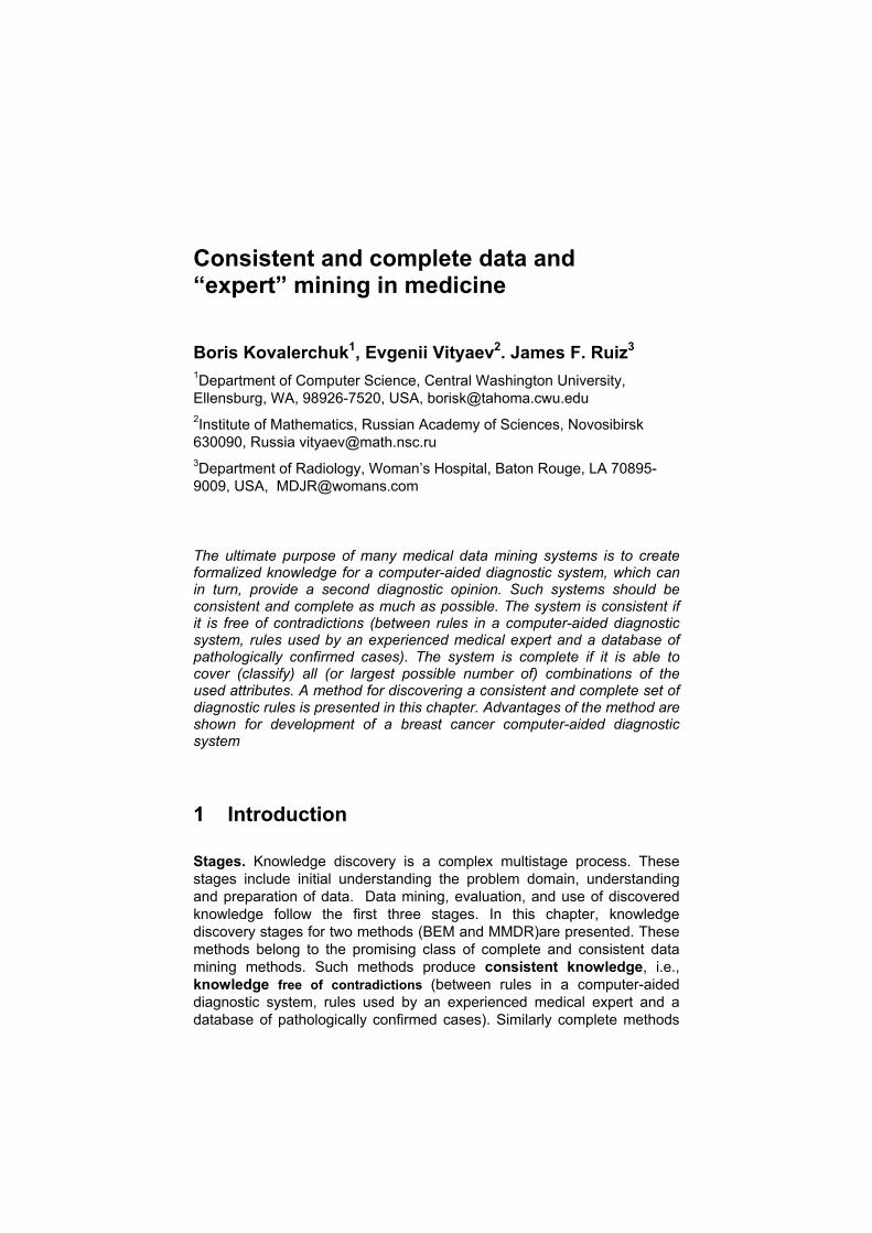
In fact, subsequently only about 40 questions were required for the two nested functions, i.e., about 20 questions per function. This number should be compared with the full search requiring 211 or 2048 questions. Therefore, this procedure allowed us to ask about 100 times fewer questions without relaxing the requirement of complete restoration of the functions.

The formal definitions of concepts from the theory of monotone Boolean functions used to obtain these results are presented in section 2.2.1.

Develop a hierarchy of Monotone Boolean functions

Present the complete function as a set of simple diagnostic rules:If A and B and C…and F Then Z

Combine functions into a complete diagnostic function

Interactively restore each function in the hierarchy

1

4

3

2

Figure 2. Major steps for extraction of expert diagnostic rules.

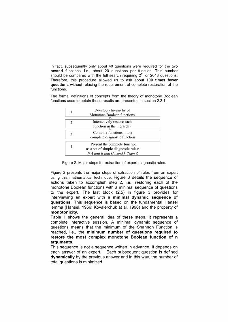
Figure 2 presents the major steps of extraction of rules from an expert using this mathematical technique. Figure 3 details the sequence of actions taken to accomplish step 2, i.e., restoring each of the monotone Boolean functions with a minimal sequence of questions to the expert. The last block (2.5) in figure 3 provides for interviewing an expert with a minimal dynamic sequence of questions. This sequence is based on the fundamental Hansel lemma (Hansel, 1966; Kovalerchuk at al. 1996) and the property of monotonicity. Table 1 shows the general idea of these steps. It represents a complete interactive session. A minimal dynamic sequence of questions means that the minimum of the Shannon Function is reached, i.e., the minimum number of questions required to restore the most complex monotone Boolean function of n arguments. This sequence is not a sequence written in advance. It depends on each answer of an expert. Each subsequent question is defined dynamically by the previous answer and in this way, the number of total questions is minimized.

.

Expert confirms monotonicity and “nesting” properties or redefine features to confirm these properties

Test expert opinion about monotonicity and “nesting” properties against cases from database

Analyze database cases that violate monotonicity and “nesting”, reject inappropriate cases

Infer function values for derivable cases without asking an expert, but using database of cases,

monotonicity and nesting properties

Interview an expert using minimal sequence of questions to completely infer a diagnostic function

using monotonicity and nesting properties

2.1

2.5

2.4

2.3

2.2

Figure 3. Iteratively restoring functions in hierarchy

Columns 2, 3 and 4 in table 1 present values of the three functions f1, f2 and ψ of five arguments chosen for this example. These functions represent regularities that should be discovered by interviewing an expert. Column 5 & 6 indicate the chain/case # for those cases that are derived as extensions of the primary vector in column 1.

These extensions are based on the property of monotonicity and so no questions are posed to the expert. Column 5 is for extending values of functions from 1 to 1 and column 6 is for extending them from 0 to 0. In other words, if f(x)=1 then column 5 helps to find y such that f(y)=1.

Similarly, column 6 works for f(x)=0 by helping to find y such that f(y)=0. Assume that each of these functions has it’s own target variable. Thus, the first question to the expert in column 2 is: “Does the sequence (01100) represent a case with the target attribute equal to 1 for f1?”

Columns 3 and 4 represent expert’s answers for functions f2 and ψ. Here (01100)=(x1, x2, x3, x4, x5). If the answer is “yes” (1), then the next question will be about the target value for the case (01010). If the answer is “No” (0), then the next question will be about the target value for (11100).

This sequence of questions is not accidental. As mentioned above, it is inferred from the Hansel lemma. An asterisk is used to indicate that the result was obtained directly from the expert.

Table 1. Dynamic sequence used to interview an expert. 1 2 3 4 5 6 7 8

Vector F1 f2 ψ Monotone extension case # Chain # Case # 1 → 1 0 → 0 (01100) 1* 1* 1* 1.2;6.3;7.3 7.1;8.1 Chain 1 1.1 (11100) 1 1 1 6.4;7.4 5.1;3.1 1.2 (01010) 1* 0* 1* 2.2;6.3;8.3 6.1;8.1 Chain 2 2.1 (11010) 1 1* 1 6.4;8.4 3.1;6.1 2.2 (11000) 1* 1* 1* 3.2 8.1;9.1 Chain 3 3.1 (11001) 1 1 1 7.4;8.4 8.2;9.2 3.2 (10010) 1* 0* 1* 4.2;9.3 6.1;9.1 Chain 4 4.1 (10110) 1 1* 1 6.4;9.4 6.2;5.1 4.2 (10100) 1* 1* 1* 5.2 7.1;9.1 Chain 5 5.1 (10101) 1 1 1 7.4;9.4 7.2;9.2 5.2 (00010) 0* 0 0* 6.2;10.3 10.1 Chain 6 6.1 (00110) 1* 1* 0* 6.3;10.4 7.1 6.2 (01110) 1 1 1 6.4;10.5 6.3 (11110) 1 1 1 10.6 6.4 (00100) 1* 1* 0* 7.2;10.4 10.1 Chain 7 7.1 (00101) 1 1 0* 7.3;10.4 10.2 7.2 (01101) 1 1 1* 7.4;10.5 8.2;10.2 7.3 (11101) 1 1 1 5.6 7.4

(01000) 0* 0 1* 8.2 10.1 Chain 8 8.1 (01001) 1* 1* 1 8.3 10.2 8.2 (01011) 1 1 1 8.4 10.3 8.3 (11011) 1 1 1 10.6 9.3 8.4 (10000) 0* 0 1* 9.2 10.1 Chain 9 9.1 (10001) 1* 1* 1 9.3 10.2 9.2 (10011) 1 1 1 9.4 10.3 9.3 (10111) 1 1 1 10.6 10.4 9.4 (00000) 0 0 0 10.2 Chain 10 10.1 (00001) 1* 0* 0 10.3 10.2 (00011) 1 1* 0 10.4 10.3 (00111) 1 1 1 10.5 10.4 (01111) 1 1 1 10.6 10.5 (11111) 1 1 1 10.6 Total Calls

13 13 12

For instance, the binary vector ((01100) could represent five binary attributes, such as positive for the disease (1) and negative for the disease

(0) for the last five-year observations of a patient. These attributes could also be months, weeks, minutes, or any other time interval.

Suppose for case #1.1 an expert gave the answer f1(01100)=0. This 0 value could be extended in column 2 for case #7.1 (00100) and case #8.1 (01000) as there is more evidence in support of f1=0. These cases are listed in column 6 in the row for case #1.1. There is no need to ask an expert about cases #7.1 and #8.1. Monotonicity is working for them.

On the other hand, the negative answer f1(01100)=0 can not be extended for f1(11100) as there is more evidence in support of f1=1. An expert should be asked about f1(11100) value.

If the answer is negative, i.e., f1(11100)=0, then this value can be extended for cases #5.1 and # 3.1. Similar to case #1.1 these cases are listed in column 6 for case #1.2.

Because of monotonicity, the value of f1 for cases #5.1 and #3.1 will also be 0. In other words, the values in column 2 for f1 are derived by up-down sliding in table 1 according to the following five steps:

Step 1.

Action: Begin with the first case #1.1, (01100). Ask the expert about the value of f1(01100).

Result: Here the expert reported that f1(01100)=1.

Step 2.

Action: Write the value for case #1.1 under column 2.

Here a "1*" is recorded next to vector (01100). Recall that an asterisk denotes an answer directly provided by the expert. The case of having the true value corresponds to column 5. (If the reply was false (0), then "0*" is written in column 2. The case of having a false value corresponds to column 6.)

Step 3. Action: Based on the response of true by the expert in step 1, check column 5 or 6 respectively to extend the given value. Here column 5 is checked as the response given for case #1.1 is true.

Result: Extend the response to the cases listed. Here cases #1.2, #6.3, and #7.3 are defined as 1. Therefore, in column 2 for cases #1.2, #6.3,

and #7.3 the values of the function f1 must be (1). Note that no asterisk is used because these are extended values.

Step 4. (Iterate until finished).

Action: Go to the next vector (called sliding down), here case #1.2. Check whether the value of f1 has already been derived. If the value of f1 is not fixed (i.e., it is empty), repeat steps 1-3, above for this new vector. If f1 is not empty (i.e., it has been already derived), then apply step 3 and slide down to the next vector. Here cases #6.4 and #7.4 are extended and then one moves to case #2.1. Note, that if the value has not yet been fixed, then it will be denoted by f1(x)=e (e for empty).

Result: Values of the function are extended. Here since for case #1.2 f1(11100) )≠e, the values of the function for the cases #6.4 and #7.4 are extended without asking an expert.

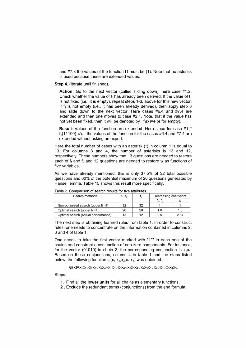
Here the total number of cases with an asterisk (*) in column 1 is equal to 13. For columns 3 and 4, the number of asterisks is 13 and 12, respectively. These numbers show that 13 questions are needed to restore each of f1 and f2 and 12 questions are needed to restore ψ as functions of five variables.

As we have already mentioned, this is only 37.5% of 32 total possible questions and 60% of the potential maximum of 20 questions generated by Hansel lemma. Table 15 shows this result more specifically.

Table 2. Comparison of search results for five attributes. Decreasing coefficient Search methods f1, f2 f2

f1, f2 ψ Non-optimized search (upper limit) 32 32 1 1 Optimal search (upper limit) 20 20 1.6 1.6 Optimal search (actual performance) 13 12 2.5 2.67

The next step is obtaining learned rules from table 1. In order to construct rules, one needs to concentrate on the information contained in columns 2, 3 and 4 of table 1.

One needs to take the first vector marked with "1*" in each one of the chains and construct a conjunction of non-zero components. For instance, for the vector (01010) in chain 2, the corresponding conjunction is x2x4. Based on these conjunctions, column 4 in table 1 and the steps listed below, the following function ψ(x1,x2,x3,x4,x5) was obtained:

ψ(x)=x1x2∨x2x3∨x2x4∨x1x3∨x1x4∨x2x3x4∨x2x3x5∨x2∨x1∨x3x4x5.

Steps:

1. Find all the lower units for all chains as elementary functions. 2 . Exclude the redundant terms (conjunctions) from the end formula.

Let us explain the concept of lower unit with an example. In chain 6 of table 1 the case #6.2 is a maximal lower unit, because f1 for this case is equal to 1 and the prior case, #6.1, has an f1 value equal to 0. Similarly, the case #6.1 will be referred to as an upper zero.

The Boolean function ψ(x) can be simplified to ψ(x)=x2∨x1∨x3x4x5.

Similarly, the target functions f1(x) and f2(x) can be obtained from columns (2 and 3) in table 1 as follows:

f1(x)= x2x3∨x2x4∨x1x2∨x1x4∨x1x3∨x3x4∨x3∨x2x5∨x1x5∨x5,

f2(x)= x2x3∨x1x2x4∨x1x2∨x1x3x4∨x1x3∨x3x4∨x3∨x2x5∨x1x5∨x4x5.

Hansel chains. This sequence of questions is not accidental. As mentioned above, it is inferred from the Hansel lemma to get a minimal number of questions in the process of restoring a complete rule. Here by complete rule we mean restoring a function for all possible inputs.

Below the general steps of the algorithm for chain construction are considered. All 32 possible cases with five binary attributes (x1, x2, x3, x4, x5) are presented in column 1 in table 1. They have been grouped according to the Hansel lemma.

These groups are called Hansel chains. The sequence of chains begins from the shortest length chain #1 -- (01100) and (11100). This chain consists only of two ordered cases (vectors), (01100) < (11100) for five binary attributes. Then largest chain #10 consists of 6 ordered cases:

(00000) < (00001) <(00011) < (00111) < (01111) < (11111).

To construct chains presented in table 1 (with five dimensions like x1, x2, x3, x4, x5) a sequential process is used, which starts with a single attribute and builds to all five attributes. A standard mathematical notation is used. For example, we will consider all five-dimensional vectors as points in 5-dimensional binary “cube”,

E5 ={0,1}x{0,1}x{0,1}x{0,1}x{0,1}.

First, all 1-dimensional chains (in E1={0,1}) are generated. Each step of chain generation consists of using current i–dimensional chains to generate (i+1) dimensional chains. Generating of chains for the next dimension (i+1) is four–step “clone-grow-cut-add” process. An i-dimensional chain is “cloned” by adding zero to all vectors in the chain. For example, the 1-dimensional chain:

(0) < (1)

clones to its two-dimensional copy:

(00) < (01).

Next we grow additional chains by changing the cloned zero to 1.

For example cloned chain 1 from above grows to chain 2:

Chain 1: (00) < (01)

Chain 2: (10) < (11).

Next we cut the head case, the largest vector (11), from chain 2 and add it as the head of chain 1 producing two Hansel 2-dimencional chains:

New chain 1: (00) < (01) <(11) and

New chain 2: (10).

This process continues through the fifth dimension for <x1, x2, x3, x4, x5>. Table 1 presents result of this process. The chains are numbered from 1 to 10 in column 7 and each case number corresponds to its chain number, e.g., #1.2 means the second case in the first chain. Asterisks in columns 2, 3 and 4 mark answers obtained from an expert.

The remaining answers for the same chain in column 2 are automatically obtained using monotonicity. The value f1(01100)=1 for case #1.1 is extended for cases #1.2, #6.3 and #7.3 in this way. Hansel chains are derived independently of the particular applied problem, they depend only on the number of attributes (five in this case).

2.2 Preparation and construction of the data and rules using MBF

2.2.1 Basic definitions and results

In this section, the formal definitions of concepts from theory of monotone Boolean functions (MBF) are presented. These concepts are used for construction of an optimal algorithm of interviewing an expert. An optimal interviewing process contains the smallest number of questions asked to obtain “artificial cases” sufficient to restore the diagnostic rules. Let En be the set of all binary vectors of length n. Let x and y be two such vectors.

Then, the vector x = (x1,x2,x3,...,xn) precedes the vector (y1,y2,y3,...,yn) (denoted as: x ≥ y) if and only if the following is true for all i=1,…,n:

xi ≥ yi

A Boolean function f(x) is monotone if for any vectors x, y ∈ En, the relation f(x) ≥ f(y) follows from the fact that x ≥ y. Let Mn be the set of all monotone Boolean functions defined on n variables.

A binary vector x of length n is said to be an upper zero of a function f(x)∈Mn, if f(x) = 0 and, for any vector y such that y ≥ x, we have f(y)=1.

Also, the term level represents the number of units (i.e., the number of the "1" elements) in the vector x and is denoted by U(x).

An upper zero x of a function f is said to be the maximal upper zero if

U(x) ≥ U(y)

for any upper zero y of the function f (Kovalerchuk and Lavkov, 1984). We define the concepts of lower unit and minimal lower unit similarly. A binary vector x of length n is said to be a lower unit of a function f(x)∈Mn, if f(x) = 1 and, for any vector y from En such that y ≥ x, we obtain f(y) = 0. A lower unit x of a function f is said to be the minimal lower unit if

U(y) ≥U(x)

for any lower unit y of the function f. The number of monotone Boolean functions of n variables, ψ(n), is given by:

))(1(

2/2)( n

nn

n εψ +

=

where

0 < ε(n) < c(logn)/n

and c is a constant (see (Alekseev, 1988; Kleitman, 1969)). Thus, the number of monotone Boolean functions grows exponentially with n.

Let a monotone Boolean function f be defined by using a certain operator Af (also called an oracle) which takes a vector x = (x1,x2,x3,...,xn) and returns the value of f(x). Let F = {F} be the set of all algorithms which can solve the above problem and let φ(F, f) be the number of accesses to the operator Af required to generate f(x) and completely restore a monotone function f∈Mn.

The Shannon function ϕ(n) (Korobkov, 1965) is defined as:

),(maxmin)( fFnnMfFϕϕ

∈∈=

F

Next consider the problem of finding all the maximal upper zeros (lower units) of an arbitrary function f∈Mn by accessing the operator Af. This set of Boolean vectors identifies a monotone Boolean function completely f.

It is shown in (Hansel, 1966) that for this problem the following relation is true (known as Hansel's lemma):

+

+

=

12/2/)(

nn

nn

nϕ (1)

Here n/2 is the closest integer number to n/2, which is no greater than n/2 (floor function).

In terms of machine learning, the set of all maximal upper zeros represents the border elements of the negative patterns. In an analogous manner, set of all minimal lower units to represent the border of positive patterns. In this way, a monotone Boolean functionrepresents two compact patterns.

Restoration algorithms for monotone Boolean functions, which use Hansel's lemma are optimal in terms of the Shannon function. That is, they minimize the maximum time requirements of any possible restoration algorithm. This lemma is one of the final results of the long-term efforts in monotone Boolean functions started by Dedekind (1897).

2.2.2 Algorithm for restoring a monotone Boolean function

Next the algorithm RESTORE is presented, for the interactive restoration of a monotone Boolean function, and two procedures GENERATE and EXPAND, for manipulation of chains.

ALGORITHM "RESTORE" f(x1,x2,...,xn)

Input: Dimension n of the binary space and access to an oracle Af . Output: A monotone Boolean function restored after a minimal number (according to formula (1)) of calls to the oracle Af.

Method: 1. Construction of Hansel chains (see section 2.2.3 below). 2. Restoration of a monotone Boolean function starting from chains of

minimal length and finishing with chains of maximal length.

This ensures that the number of calls to the oracle Af is no more than the limit presented in formula (1).

Table 2. Procedure RESTORE

Set i=1; {initialization} DO WHILE (function f(x) is not entirely restored) Step 1: Use procedure GENERATE to generate element ai; which is a binary vector. Step 2: Call oracle Af to retrieve the value of f(aI);

Step 3: Use procedure EXPAND to deduce the values of other elements in Hansel chains (i.e., sequences of examples in En) by using the value of f(ai ), the structure of element ai and the monotonicity property of monotonicity. Step 4: Set i → i+1; RETURN

PROCEDURE "GENERATE": Generate i-th element ai to be classified by the oracle Af.

Input: The dimension n of the binary space. Output: The next element to send for classification by the oracle Af. Method: Begin with the minimal Hansel chain and proceed to maximal Hansel chains.

Table 3. Procedure GENERATE IF i=1 THEN {where i is the index of the current element} Step 1.1: Retrieve all Hansel chains of minimal length; Step 1.2: Randomly choose the first chain C1 among the chains retrieved in step 1.1; Step 1.3: Set the first element a1 as the minimal element of chain C1; ELSE Set k=1 {where k is the index number of a Hansel chain}; DO WHILE (NOT all Hansel chains are tested) Step 2.1: Find the largest element ai of chain Ck, which still has no f(ai) value; Step 2.2: If step 2.1 did not return an element ai then randomly select the next Hansel Chain Ck+1 of the same length l as the one of the current chain Ck; Step 2.3: Find the least element ai from chain Ck+1, which still has no f(ai) value; Step 2.4: If Step 2.3 did not return an element ai, then randomly choose chain Ck+1 of the next available length (l+1); Step 2.5: Set k ← k+1;

PROCEDURE "EXPAND": Assign values of f(x) for x ≤ ai or x ≥ ai in chains of the given length l and in chains of the next length l+2. According to the Hansel lemma if for n the first chain has an even length then all other chains for this n will be even. A similar result holds for odd lengths.

Input. The f(ai) value. Output. n extended set of elements with known f(x) values. Method: The method is based on monotone properties:

if x ≥ ai and f(ai)=1, then f(x)=1; and

if ai ≥ x and f(ai)=0, then f(x)=0.

Table.4. Procedure EXPAND

Step 1. Obtain x such that x ≥ai or x ≥ai and x is in a chain of the lengths l or l+2. Step 2. If f(aI)=1, then for all x such that x ≥aI set f(x)=1; If f(aI)=0, then for all x such that aI ≥x set f(x)=0; Step 3: Store the f(x) values which were obtained in step 2;

2.2.3 Construction of Hansel Chains

Several steps in the previous algorithms deal with Hansel chains. Next we describe how to construct all Hansel chains for a given space En of dimension n. First, we give a formal definition of a general chain. A chain is a sequence of binary vectors a1, a2 ,...ai, ai+1,..., a,i such that ai+1 is obtained from ai by changing a "0" element to a "1". That is, there is an index k such that ai,k = 0, ai+1,k = 1 and for any t≠k, the following is true ai,t=ai+1,t. For instance, the following list of three vectors is a chain <01000, 01100, 01110>. To construct all Hansel chains, we will use an iterative procedure as follows. Let En ={0,1}n be the n-dimensional binary cube. All chains for En are constructed from chains for En-1. Therefore, we begin the construction for En by starting with E1 and iteratively proceeding to En.

Chains for E1.

For E1 there is only a single (trivial) chain and it is <(0), (1)>.

Chains for E2.

First we consider E1 and add at the beginning of each one of its chains the element (0). Thus, we obtain the set {00, 01}. This set is called E2

min. In addition, by changing the first "0" to “1” in E2

min, we construct the set E2max

= {10, 11}. To simplify notation, we will usually omit "( )" for vectors as (10) and (11). Both E2

min and E2max are isomorphic to E1, clearly,

E2 = E2min ∪ E2

max.

However, they are not Hansel chains. To obtain Hansel chains we need to modify them as follows: Adjust the chain <00, 01> by adding the maximum element (11) from the chain <10, 11>. That is, obtain a new chain <00, 01, 11>. Then we need to remove element (11) from the chain <10, 11>. Thus, we obtain the two new chains: <00, 01, 11> and <10>. These chains are the Hansel chains for E2. That is E2 = {<00, 01, 11>, <10>}.

Chains for E3.

The Hansel chains for E3 are constructed in a manner similar to the chains for E2. First, we double (clone) and adjust (grow) the Hansel chains of E2 to obtain E3

min and E3max. The following relation is also true:

E3 = E3min ∪ E3

max,

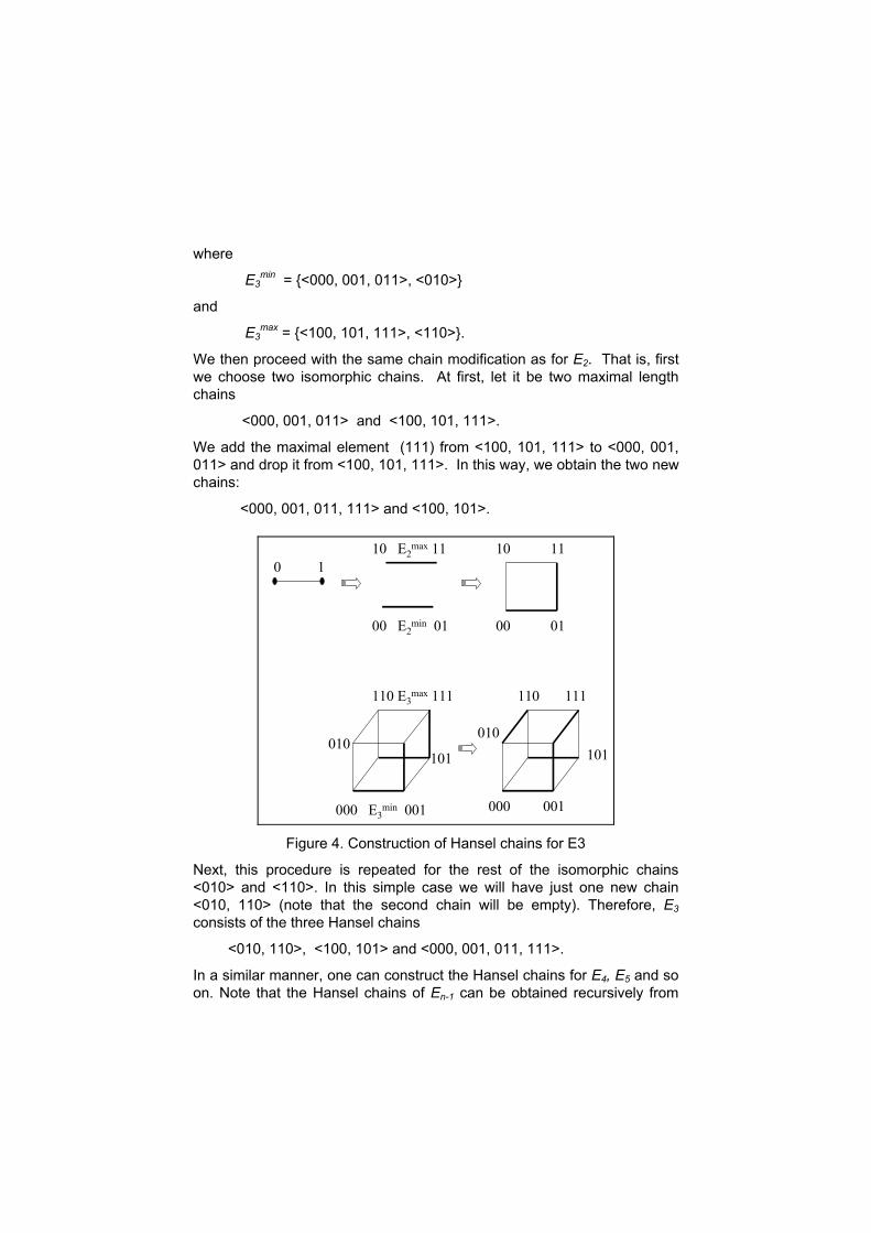
where

E3min = {<000, 001, 011>, <010>}

and

E3max = {<100, 101, 111>, <110>}.

We then proceed with the same chain modification as for E2. That is, first we choose two isomorphic chains. At first, let it be two maximal length chains

<000, 001, 011> and <100, 101, 111>.

We add the maximal element (111) from <100, 101, 111> to <000, 001, 011> and drop it from <100, 101, 111>. In this way, we obtain the two new chains:

<000, 001, 011, 111> and <100, 101>.

10 E2max 11

00 E2min 01 00 01

10 110 1

000 E3min 001

110 E3max 111

101010

000 001

110 111

101010

Figure 4. Construction of Hansel chains for E3

Next, this procedure is repeated for the rest of the isomorphic chains <010> and <110>. In this simple case we will have just one new chain <010, 110> (note that the second chain will be empty). Therefore, E3 consists of the three Hansel chains

<010, 110>, <100, 101> and <000, 001, 011, 111>.

In a similar manner, one can construct the Hansel chains for E4, E5 and so on. Note that the Hansel chains of En-1 can be obtained recursively from

the Hansel chains of E1, E2,...,En-2. Figure 4 depicts the above issues for the E1, E2 and E3 spaces.

3 Preparation of data

3.1 Problem outline

Below we discuss the application of above described methods for medical diagnosis using features extracted from mammograms. In the U.S., breast cancer is the most common female cancer (Wingo et a1. 1995). The most effective tool in the battle against breast cancer is screening mammography. However, it has been found that intra- and inter-observer variability in mammographic interpretation is significant (up to 25%) (Elmore et al. 1994). Additionally, several retrospective analyses have found error rates ranging from 20% to 43%. These data clearly demonstrate the need to improve the reliability of mammographic interpretation.

The problem of identifying cases suspicious for breast cancer using mammographic information about clustered calcifications is considered. Examples of mammographic images with clustered calcifications are shown in figures 6-8. Calcifications are seen in most mammograms and commonly indicate the presence of benign fibrocystic change. However, certain features can indicate the presence of malignancy. Figures 5-7 illustrate the broad spectrum of appearances that might be present within a mammogram. Figure 5 shows calcifications that are irregular in size and shape. These are biopsy proven malignant type calcifications.

Figure 5. Clustered calcifications produced by breast cancer. Calcifications display irregular contours and vary in size and shape.

Figure 6 presents a cluster of calcifications within a low-density ill-defined mass. Again, these calcifications vary in size, shape and density suggesting that a cancer has produced them. Finally, Figure 7 is an example of a carcinoma, which has produced a high-density nodule with irregular spiculated margins. While there are calcifications in the area of this cancer, the calcifications are all nearly spherical in shape and quite in uniform in their density. This high degree of regularity suggests a benign origin. At biopsy, the nodule proved to be a cancer while the calcifications were associated with a benign fibrocystic change. There is promising Computer-Aided diagnostic research aimed to improve the situation (Shetrn, 1996; SCAR, 1998; TIWDM, 1996, 1998; CAR, 1996).

Figure 6. Low density, ill defined mass and associated calcifications.

Figure 7. Carcinoma producing mass with spiculated margins and associated benign calcifications.

3.2 Hierarchical Approach

The interview of a radiologist to extract (“mine”) breast cancer diagnostic rules is managed using an original method described in the previous

section. One can ask a radiologist to evaluate a particular case when a number of features take on a set of specific values. A typical query will have the following format:

"If feature 1 has value V1, feature 2 has value V2,..., feature n has value Vn, then should biopsy be recommended or not?

Or, does the above setting of values correspond to a case suspicious of cancer or not?"

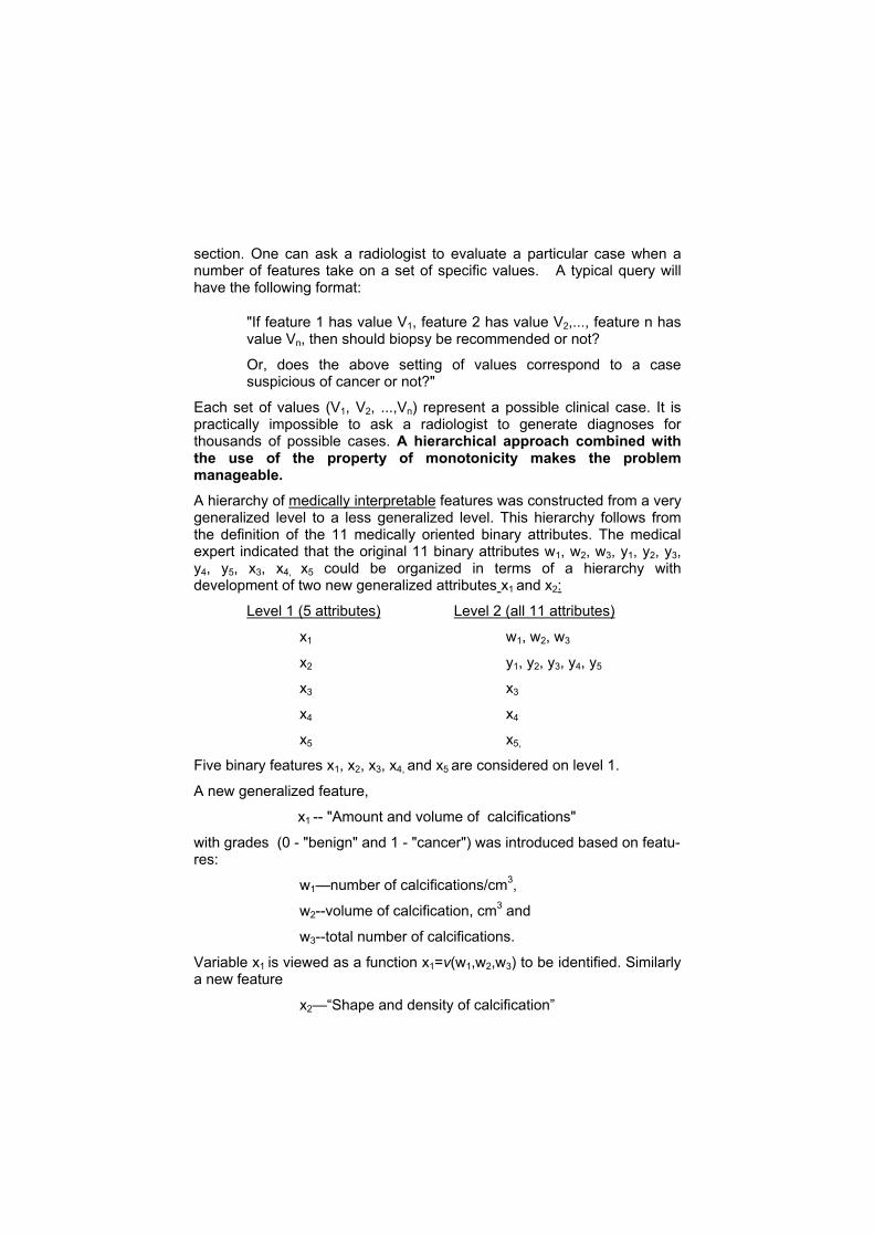
Each set of values (V1, V2, ...,Vn) represent a possible clinical case. It is practically impossible to ask a radiologist to generate diagnoses for thousands of possible cases. A hierarchical approach combined with the use of the property of monotonicity makes the problem manageable. A hierarchy of medically interpretable features was constructed from a very generalized level to a less generalized level. This hierarchy follows from the definition of the 11 medically oriented binary attributes. The medical expert indicated that the original 11 binary attributes w1, w2, w3, y1, y2, y3, y4, y5, x3, x4, x5 could be organized in terms of a hierarchy with development of two new generalized attributes x1 and x2:

Level 1 (5 attributes) Level 2 (all 11 attributes)

x1 w1, w2, w3

x2 y1, y2, y3, y4, y5

x3 x3

x4 x4

x5 x5,

Five binary features x1, x2, x3, x4, and x5 are considered on level 1.

A new generalized feature,

x1 -- "Amount and volume of calcifications"

with grades (0 - "benign" and 1 - "cancer") was introduced based on featu-res:

w1—number of calcifications/cm3,

w2--volume of calcification, cm3 and

w3--total number of calcifications.

Variable x1 is viewed as a function x1=v(w1,w2,w3) to be identified. Similarly a new feature

x2—“Shape and density of calcification”

with grades: (1) for "marked" and (0) for "minimal" or, equivalently (1)-"cancer" and (0)-"benign" generalizes features:

y1 -- "Irregularity in shape of individual calcifications"

y2 -- "Variation in shape of calcifications"

y3 -- "Variation in size of calcifications"

y4 -- "Variation in density of calcifications"

y5 -- "Density of calcifications".

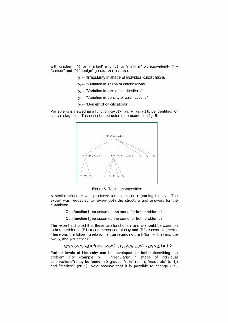
Variable x2 is viewed as a function x2=ψ(y1, y2, y3, y4, y5) to be identified for cancer diagnosis. The described structure is presented in fig. 9.

x1= ν(w1, w2, w3) x2=ψ(y1, y2, y3, y4, y5) x3 x4 x5

fi(x1,x2,x3,x4,x5)

w1 w2 w3 y1 y2 y3 y4 y5

Figure 8. Task decomposition

A similar structure was produced for a decision regarding biopsy. The expert was requested to review both the structure and answers for the questions:

“Can function f1 be assumed the same for both problems?

“Can function f2 be assumed the same for both problems?

The expert indicated that these two functions v and ψ should be common to both problems: (P1) recommendation biopsy and (P2) cancer diagnosis. Therefore, the following relation is true regarding the fi (for i = 1, 2) and the two ϕ, and ψ functions:

fi(x1,x2,x3,x4,x5) = fi(v(w1,w2,w3), ψ(y1,y2,y3,y4,y5), x3,x4,x5), i = 1,2.

Further levels of hierarchy can be developed for better describing the problem. For example, y1 ("irregularity in shape of individual calcifications") may be found in 3 grades: "mild" (or t1), "moderate" (or t2) and "marked" (or t3). Next observe that it is possible to change (i.e.,

generalize) the operations used in the function ψ(y1,y2,..,y5). For instance, we may have mentioned function ψ as follows: ψ(y1,y2,..,y5) = y1 & y2 ∨ y3 & y4 & y5, where & and ∨ are the binary, logical operations for "AND" and "OR", respectively. Then, & and ∨ can be substituted for one of their multivalued logic analogs, for example, x & y = min(x,y) and x ∨ y = max(x,y) as in fuzzy logic (see, for example in (Kovalerchuk and Talianski, 1992) ). This decomposition is presented in fig. 4.

Assume that x1 is the number and the volume occupied by calcifications, in a binary setting, as follows: (0-"against cancer", 1-"for cancer"). Similarly, let:

x2--{shape and density of calcifications}, with values: 0-"benign", 1-"cancer"

x3--{ductal orientation}, with values: 0-"benign", 1-"cancer"

x4--{comparison with previous examination}, with values: 0-"benign",1-"cancer"

x5--{associated findings}, with values: 0-"benign",1-"cancer".

3.3 Monotonicity

To understand how monotonicity is applied in the breast cancer problem, consider the evaluation of calcifications in a mammogram. Given the above definitions we can represent clinical cases in terms of binary vectors with five generalized features as: (x1,x2,x3,x4,x5). Next consider the two clinical cases that are represented by the two binary sequences: (10110) and (10100). If one is given that a radiologist correctly diagnosed (10100) as a malignancy, then, by utilizing the property of monotonicity, we can also conclude that the clinical case (10110) should also be a malignancy.

This conclusion is based on the systematic coding of all features “suggestive for cancer” as 1. Observe that (10100) has two indications for cancer:

x3=1 (ductal orientation having value of 1; suggesting cancer) and

x1=1 (amount and volume of calcifications with value 1 indicating cancer).

In the second clinical case we have these two observations for cancer and also x4=1 (a comparison with previous examinations suggesting cancer). In the same manner if (01010) is not considered suspicious for cancer, then the case (00000) should also not be considered suspicious. This is true because in the second case we have less evidence indicating the presence of cancer. The above considerations are the essence of how our algorithms function. They can combine logical analysis of data with

monotonicity and generalize accordingly. In this way, the weaknesses of the brute-force methods can be avoided.

It is assumed that if the radiologist believes that the case is malignant, then he/she will recommend a biopsy. More formally, these two sub-problems are defined as follows:

The Clinical Management Sub-Problem (P1): One and only one of the following two disjoint outcomes is possible:

1) "Biopsy is necessary", or:

2) "Biopsy is not necessary".

The Diagnosis Sub-Problem (P2): Similarly as above, one and only one of two following disjoint outcomes is possible. That is, a given case is:

1) "Suspicious for malignancy", or:

2) "Not suspicious for malignancy".

The goal here is to extract the way the system operates in the form of two discriminant Boolean functions f2 and f1:

1. Function f1 returns true (1) value if the decision is "biopsy is necessary", false (0) otherwise.

2. Function f2 returns true (1) value if the decision is "suspicious for malignancy", false (0) otherwise.

The first function is related to the first sub-problem, while the second function is related to the second sub-problem. There is an important relation between these two sub-problems P1 and P2 and functions f1(α), f2(α). The problems are nested, i.e., if the case is suggestive of cancer (f2(α)=1) then biopsy should be recommended (f1(α)=1) for this case, therefore, f2(α)=1 ⇒ f1(α)=1. Also if biopsy is not recommended (f1(α)=0) then the case is not suggestive of cancer (f2(α)=0), therefore f1(α)=0 ⇒ f2(α)=0. The last two statements are equivalent to f2(α) ≥ f1(α) and f1(α) ≤ f2(α), respectively for case α. Let E+

n,1, is a set of α sequences from En, such that f1(α)=1 (biopsy positive cases). Similarly, E+

n,2 is a set of α sequences from En, such that f2(α)=1 (cancer positive cases). Observe, that the nested property formally means that E+

n2 ⊆ E+n1 (for all cases

suggestive of cancer, biopsy should be recommended) and f2(α) ≥ f1(α) for all ∈En.

The previous two interrelated sub-problems P1 and P2 can be formulated as a restoration problem of two nested monotone Boolean functions f1 and f2. A medical expert was presented with the ideas of monotonicity and nested functions as above and he felt comfortable with the idea of using nested monotone Boolean functions. Moreover, dialogue that followed confirmed the validity of this assumption. Similarly, the function

x2=ψ(y1, y2, y3, y4, y5) for x2 (“Shape and density of calcification”) was confirmed to be a monotone Boolean function.

A Boolean function is a compact presentation of a set of diagnostic rules. A Boolean discriminant function can be presented in the form of a set of logical “IF-THEN” rules, but it is not necessary that these rules stand for a single tree as in the decision tree method. A Boolean function can produce a diagnostic discriminant function, which cannot be produced by the decision tree method. For example, the Biopsy Sub-Problem is stated:

f1(x)=x2x4∨x1x2∨x1x4∨x3∨x5 (2)

This formula is read as follows

IF (x2 AND x4) OR (x1 AND x2) OR (x1 AND x4) OR (x3) OR (x5)

THEN Biopsy is recommended

In medical terms this translates as:

IF (shape and density of calcifications suggests cancer AND comparison with previous examination suggests cancer) OR (the number and the volume occupied by calcifications suggests cancer AND shape and density of calcifications suggests cancer) OR (the number and the volume occupied by calcifications suggests cancer AND comparison with previous examination suggests cancer) OR (ductal orientation suggests cancer) OR (associated findings suggests cancer)

THEN Biopsy is recommended.

As was already mentioned in section 2, full restoration of either one of the functions f1 and f2 with 11 arguments without any optimization of the interview process would have required up to 2048 calls to the medical expert. Note that practically all studies in breast cancer computer-aided diagnostic systems derive diagnostic rules using significantly less than 1,000 cases (Gurney, 1994). Using the Hansel lemma restoring a monotone Boolean would require at most 924 calls to a medical expert. However, this upper limit of 924 calls can be reduced further. The hierarchy presented in fig. 9 reduces the maximum number of questions needed to restore Monotone Boolean functions of 11 binary variables to 72 questions (non-deterministic questioning) and to 46 using Hansel lemma. The actual number of questions asked was about 40, including both nested functions (cancer and biopsy) (i.e., about 20 questions per function).

3.4 Rules “mined” from expert

Examples of Extracted Diagnostic Rules. Below examples of rules discovered using technique described in previous sections are presented. EXPERT RULE (ER1):

IF NUMBER of calcifications per cm2 (w1) is large

AND TOTAL number of calcifications (w3) is large

AND irregularity in SHAPE of individual calcifications is marked THEN suspicious for malignancy EXPERT RULE 2 (ER2):

IF NUMBER of calcifications per cm2 (w1) large

AND TOTAL number of calcifications is large (w3)

AND variation in SIZE of calcifications (y3) is marked

AND VARIATION in Density of calcifications (y4) is marked

AND DENSITY of calcification (y5) is marked

THEN suspicious for malignancy.

EXPERT RULE 3 (ER3):

IF (SHAPE and density of calcifications are positive for cancer

AND Comparison with previous examination is positive for cancer)

OR (the number and the VOLUME occupied by calcifications are

positive for cancer

AND SHAPE and density of calcifications are positive for cancer)

OR (the number and the VOLUME occupied by calcifications are positive for cancer AND comparison with previous examination is positive for cancer)

OR (DUCTAL orientation is positive for cancer OR associated

FINDINGS are positive for cancer)

THEN Biopsy is recommended. In addition, some other rules were extracted. Below these rules are presented briefly in formal notation. MAL stands for suspicious for malignancy.

IF w2&y1 THEN MAL IF w2&y2 THEN MAL IF w2&y&3&y4&y5 THEN MAL IF w1&w3&y2 THEN MAL

IF w1&w3&x5 THEN MAL

3.5 Rule extraction through monotone Boolean functions

Boolean expressions were obtained for shape and density of calcification (see figure 8 for data structure) from the information depicted in table 1 (columns 1 and 4) with the following steps:

(i) Find all the maximal lower units for all chains as elementary conjunctions;

(ii) Exclude the redundant terms (conjunctions) from the end formula. See expression (3) below. Thus, from table 1 (columns 1 and 4) the following formula was obtained

x2=ψ(y1, y2, y3, y4, y5) =y1y2y2y3∨y2y4∨y1y3∨y1y4∨y2y3y4∨y2y3y5∨y2∨y1∨y3y4y5

and then we simplified it to y2∨y1∨y3y4y5. As above, from columns 2 and 3 in table 1 we obtained the initial components of the target functions of x1, x2, x3, x4, x5 for the biopsy sub-problem as follows:

f1(x) = x2x3∨ x2x4∨x1x2∨x1x4∨x1x3∨x3x4∨x3∨x2x5∨x1x5∨x5,

and for the cancer sub-problem to be defined as:

f2(x) = x2x3∨x1x2x4∨x1x2∨x1x3x4∨x1x3∨x3x4∨x3∨x2x5∨x1x5∨x4x5.

The simplification of these disjunctive normal form (DNF) expressions allowed us to exclude redundant conjunctions and produce DNFs. For instance, in x2 the term y1y4 is not necessary, because y1 covers it.

Using this technique we extracted 16 rules for the diagnostic class "suspicious for malignancy" and 13 rules for the class "biopsy” (see formulas (6) and (7) for mathematical representation).

All of these rules are obtained from formula (6) presented below. Similarly, for the second sub-problem (highly suspicious for cancer) the function that we found was:

f2(x) = x1x2∨x3∨ (x2∨x1∨x4)x5 (3)

Regarding the second level of the hierarchy (which recall has 11 binary features) we interactively constructed the following functions (interpretation of the features is presented below):

x1=v(w1,w2,w3)=w2∨w1w3 (4)

and

x2=ψ(y1,y2,y3,y4,y5)=y1∨y2∨y3y4y5 (5)

By combining the functions in (2)-(5) the formulas of all 11 features for biopsy are obtained:

f1(x)=(y2∨y1∨y3y4y5)x4∨(w2∨w1w3)(y2∨y1∨y3y4y5) ∨ (w2∨w1w3)x4∨x3∨x5 (6)

and for suspicious for cancer:

f2(x)=x1x2∨x3∨(x2∨x1∨x4)x5=(w2∨w1w3)(y1∨y2∨y3y4y5)∨x3∨(y1∨y2∨y3y4y5)

∨(w2∨w1w3∨x4) (7)

4 Data mining

4.1 Relational data mining method

A machine learning method called Machine Methods for Discovering Regularities (MMDR) (Vityaev et al. 1992;1993; 1998; Kovalerchuk and Vityaev, 1998; 1999; 2000) can be applied for the discovery of diagnostic rules for breast cancer diagnosis. The method expresses patterns as relations in first order logic and assigns probabilities to rules generated by composing patterns.

Learning systems based on first-order representations have been successfully applied to many problems in chemistry, physics, medicine, finance and other fields (Kovalerchuk et al, 1984; 1992; 1997; 1998; Kovalerchuk, Ruiz and Vityaev, 1997;1998;1999; Vityaev et al. 1992; 1993; 1998). As any technique based on logic rules, this technique allows one to obtain human-readable forecasting rules that are (Mitchell, 1997) interpretable in medical language and it provides a presumptive diagnosis. A medical specialist can evaluate the correctness of the presumptive diagnosis as well as a diagnostic rule.

The critical issue in applying data-driven forecasting systems is generalization. MMDR and related “Discovery” software systems (Vityaev et al, 1992;1993;1998) generalize data through “law-like” logical probabilistic rules. Conceptually, law-like rules came from the philosophy of science. These rules attempt to mathematically capture the essential features of scientific laws: (1) high level of generalization; (2) simplicity (Occam’s razor); and, (3) refutability. The first feature -- generalization -- means that any other regularity covering the same events would be less general, i.e., applicable only to a subset of events covered by the law-like

regularity. The second feature – simplicity--reflects the fact that a law-like rule is shorter than other rules. The law-like rule (R1) is more refutable than another rule (R2) if there are more testing examples which refute (R1) than (R2), but the examples fail to refute (R1).

Formally, an IF-THEN rule C is presented as

A1& …&Ak ⇒ A0,

where the IF-part, A1&...&Ak, consists of true/false logical statements A1,…,Ak, and the THEN-part consists of a single logical statement A0. Statements Ai are some given refutable statements or their negations, which are also refutable. Rule C allows one to generate sub-rules with a truncated IF-part, e.g. A1&A2 ⇒ A0 , A1&A2&A3 ⇒ A0 and so on. It is known that a sub-rule is logically stronger than the rule used to construct the sub-rule. Thus, if some rule and its sub-rule C’ classify correctly the same set of examples, then the sub-rule is preferred. In general, there are three reasons to prefer the sub-rule: 1. The sub-rule is more general (logically stronger and describes the

same set of events). 2. The sub-rule is simpler then the rule, because it consists of fewer

statements in the IF-part. 3. Sub-rule is better testable (more refutable) then the rule, because the

larger set of possible examples may falsify it (the IF-part of the sub-rule is less restrictive).

Thus, if a rule covers the set of examples then one can test that no one of its sub-rules also covers the same set of examples. Otherwise, this sub-rule or maybe some of its sub-rules will be preferred, because this sub-rule is simpler, more general and more refutable. In deterministic case, a “law-like” rule can be defined (for some set of examples) as a rule without sub-rules covering this set of examples. In other words, “law-like” rule is the rule, which is true for some set of examples, but no one of its sub-rule is true for this data.

If examples contain noise, which is typical in medical field, the probabilistic characteristics of the expressions are used instead of crisp (true/false) values. The conditional probability of the rule is used in the MMDR method as this charateristic. For rule C, its conditional probability Prob(C) = Prob(A0/A1&...&Ak) is defined, assuming that Prob(A1&...&Ak) > 0. Similarly conditional probabilities Prob(A0/ Ai1&...&Aih) are defined for sub-rules Ci, such as Ai1& …&Aih ⇒ A0., assuming that Prob(Ai1&...&Aih) > 0.

Conditional probability, Prob(C) = Prob(A0/A1&...&Ak), is used for estimating forecasting power of the rule to predict A0. In addition, the conditional probability is a major tool for defining non-deterministic (probabilistic) law-like rules (regularities) (Vityaev E et al. 1998;1992).

The rule is a probabilistic “law-like” rule iff all of its sub-rules have a statistically significant lower conditional probability than the rule. Another definition of “law-like” rules can be given in terms of generalization. The rule is “law-like” iff it can not be generalized without producing a statistically significant reduction in its conditional probability. “Law-like” rules defined in this way hold all three listed above properties (properties of scientific laws), i.e., these rules are (1) general from a logical perspective, (2) simple, and (3) refutable. Section 5 presents some breast cancer diagnostic rules extracted using this approach.

The “Discovery” software searches all chains C1 , C2 , …, Cm-1, Cm of nested “law-like” subrules, where C1 is a subrule of rule C2 , C1 = sub(C2), C2 is a subrule of rule C3, C2 = sub(C3) and finally Cm-1 is a subrule of rule Cm, Cm-1 = sub(Cm). Also

Prob(C1) < Prob(C2), … , Prob(Cm-1) < Prob(Cm).

There is a theorem (completeness theorem, Vityaev, 1992) that all rules, which have a maximum value of conditional probability, can be found at the end of such chains. The algorithm stops generating new rules when they become too complex (i.e., statistically insignificant for the data) even if the rules are highly accurate on training data. The Fisher statistical criterion is used in this algorithm for testing statistical significance. The obvious other stop criterion is time limitation.

Theoretical advantages of MMDR generalization are presented in (Vityaev et al. 1992;1993;1998, Kovalerchuk and Vityaev, 2000). This approach has some similarity with the hint approach (Abu-Mostafa, 1990). We use mathematical formalisms of first-order logic rules described in (Russel and Norvig, 1995; Halpern, 1990; Krantz et al. 1971; 1989; 1990). Note that a class of general propositional and first-order logic rules, covered by MMDR is wider than a class of decision trees (Mitchell, 1997).

Figure 9 describes the steps of MMDR. In the first step we select and/or generate a class of logical rules suitable for a particular task. The next step is learning the particular first-order logic rules using available training data. Then we test first-order logic rules on training data using Fisher statistical criterion.

After that statistically significant rules are selected and Occam’s razor principle is applied: the simplest hypothesis (rule) that fits the data is preferred (Mitchell, 1997). The last step is creating interval and threshold forecasts using selected logical rules: IF A(x,y,…,z) THEN B(x,y,…,z).

MMDR models (selecting/generating logical rules

with variables x,y,..,z:IF A(x,y,…,z)THEN B(x,y,…,z)

Learning logical rules on training data using conditional

probabilities of inference P(B(x,y,…,z)/A(x,y,…z))

Creating interval and threshold forecasts using rules

IF A(x,y,…,z) THEN B(x,y,…,z) and p-quintiles

Testing and selecting logical rules (Occam’s razor, Fisher criterion)

Figure 9. Flow diagram for MMDR: steps and technique applied

4.2 Mining diagnostic rules from breast cancer data

The next task is the discovery of rules from data. This study was accomplished using an extended set of features. A set of features listed in section 3.2 was extended with two features:

- Le Gal type and

- Density of parenchyma

with three diagnostic classes:

1. "malignant"

2. "high risk of malignancy" and

3. "benign".

Several dozen diagnostic rules were extractred with statistical significant on the 0.01, 0.05 and 0.1 levels (F-criterion).

These rules are based on 156 cases (73 malignant, 77 benign, 2 highly suspicious and 4 with mixed diagnosis). In the Round-Robin test the rules diagnosed 134 cases and refused to diagnose 22 cases.

The total accuracy of diagnosis is 86%. Incorrect diagnoses were obtained in 19 cases (14% of diagnosed cases). The false-negative rate was 5.2% (7 malignant cases were diagnosed as benign) and the false-positive rate was 8.9% (12 benign cases were diagnosed as malignant). Some of the

rules are shown in table 5. This table resents examples of discovered rules with their statistical significance.

Table 5. Examples of extracted diagnostic rules Diagnostic rule

F-criterion for features

Total significance of F-criterion

Accuracy of diagno-sis for test cases (%)

0.01 0.05 0.1

IF NUMber of calcifications per cm2 is between 10 and 20 AND VOLume > 5 cm3 THEN Malignant

NUM VOL

0.003 0.004

+ +

+ +

+ +

93.3

IF TOTal number of calcifications >30 AND VOLume > 5 cm3 AND DENsity of calcifications is moderate THEN Malignant

TOT VOL DEN

0.023 0.012 0.033

- - -

+ + +

+ + +

100.0

IF VARiation in shape of calcifications is marked AND NUMber of calcifications is between 10 and 20 AND IRRegularity in shape of calcifications is moderate THEN Malignant

VAR NUM IRR

0.004 0.004 0.025

+ + -

+ + +

+ + +

100.0

IF variation in SIZE of calcifications is moderate AND Variation in SHAPE of calcifications is mild AND IRRegularity in shape of calcifications is mild THEN Benign

SIZE SHAPE IRR

0.015 0.011 0.088

- - -

+ + -

+ + +

92.86

Figure 10 presents results for another selection criterion: level of conditional probability of rules. Three groups of rules marked MMDR1, MMDR2 and MMDR3 with levels 0.7, 0.85 and 0.95 are used in this figure. A higher level of conditional probability decreases the number of rules and diagnosed patients, but increases accuracy of diagnosis.

Group MMDR1 contains extracted 44 statistically significant rules for 0.05 level of F –criterion with a conditional probability no less than 0.70. Group MMDR2 consists of 30 rules with a conditional probability no less than 0.85 and 18 rules with a conditional probability no less than 0.95 form MMDR3. The total accuracy of diagnosis is 82%. The false negative rate is 6.5% (9 malignant cases were diagnosed as benign) and the false positive rate was 11.9% (16 benign cases were diagnosed as malignant).

The most reliable 30 rules delivered a total accuracy of 90%, and the 18 most reliable rules performed with 96.6% accuracy with only 3 false positive cases (3.4%).

Neural Network (“Brainmaker”, California Scientific Software) software had given 100% accuracy on training data, but for the Round-Robin test, the total accuracy fell to 66%.

The main reason for this low accuracy is that Neural Networks (NN) do not evaluate the statistical significance of the perfect performance (100%) on training data. Poor results (76% on training data test) were also obtained with Linear Discriminant Analysis (“SIGAMD” software, StatDialogue software, Moscow).

0.5

0.6

0.7

0.8

0.9

1

MMDR3 MMDR2 MMDR1 Neural Network

% true cancer

% true benign

% classified

total accuracywithout refused

Figure 11. Performance of methods (Round-Robin test)

Figure 10. Performance of methods (Round-Robin test)

The Decision Tree approach (“SIPINA” software, Université Lumière, Lyon, France) performed with accuracy of 76%-82% on training data. This is worse than what we obtained for the MMDR method with the much more difficult Round-Robin test (fig. 10). The very important false-negative rate was 3-8 cases (MMDR), 8-9 cases (Decision Tree), 19 cases (Linear Discriminant Analysis) and 26 cases (NN).

In these experiments, rule-based methods (MMDR and decision trees) outperformed other methods. Note also that only MMDR and decision trees produce diagnostic rules. These rules make a computer-aided diagnostic decision process visible, transparent to radiologists. With these methods radiologists can control and evaluate the decision making process.

Linear discriminant analysis gives an equation, which separates benign and malignant classes. For example,

0.0670x1-0.9653x2+…

represents a case. How would one interpret a weighted number of calcifications/cm2 (0.0670x1) plus a weighted volume (cm3), i.e., 0.9653x2 ? There is no direct medical sense in this arithmetic.

5 Evaluation of discovered knowledge

Below we compare some rules extracted from 156 cases using data mining algorithms and by interviewing the radiologist.

From the database the rule DBR1 was extracted:

IF NUMber of calcifications per cm2 (w1) is between 10 and 20

AND VOLume (w2)>5 cm3

THEN Malignant

The closest expert rule is ER1:

IF NUMber of calcifications per cm2 (w1) large

AND TOTal number of calcifications (w3) is large AND

irregularity in SHAPE of individual calcifications (y1) is marked

THEN Malignant

There is no rule DBR1 among the expert rules, but this rule is statistically significant (0.01, F-criterion). Rule DBR1 should be tested by the radiologist and included in diagnostic knowledge base after his verification. The same verification procedure should be done for ER1.

This rule should be analyzed against database of real cases. The analysis may lead to conclusion that the database is not sufficient and rule DB1 should be extracted from the extended database. Also, the radiologist can conclude that the feature set is not sufficient to incorporate rule DBR1 in to his knowledge base. This kind of analysis is not possible for Linear Discriminant analysis or Neural Networks. We also use fuzzy logic to clarify the meaning of such concepts as "Total number of calcifications (w3) is large". The reliability of the expert radiologist against 30 actual cases was tested. The radiologist classified these cases into three categories:

1. "High probability of Cancer, Biopsy is necessary" (or CB).

2. "Low probability of cancer, probably Benign but Biopsy/short term follow-up is necessary" (or BB).

3. "Benign, biopsy is not necessary" (or BO).

These cases were selected from screening cases recalled for magnification views of calcifications. For the CB and BB cases, pathology reports of biopsies confirmed the diagnosis while a two-year follow-up had been used to confirm the benign status of BO.

The expert's diagnosis was in full agreement with his extracted diagnostic rules for 18 cases and for 12 cases he asked for more information than that given in the extracted rule. When he was interviewed he answered that he had cases with the same combination of 11 features but with different diagnosis. This suggests that we need to extend the feature set and the rule set to adequately cover complicated cases. Restoration of Monotone Boolean functions allowed us to identify this need. This is one of the useful outputs from these functions.

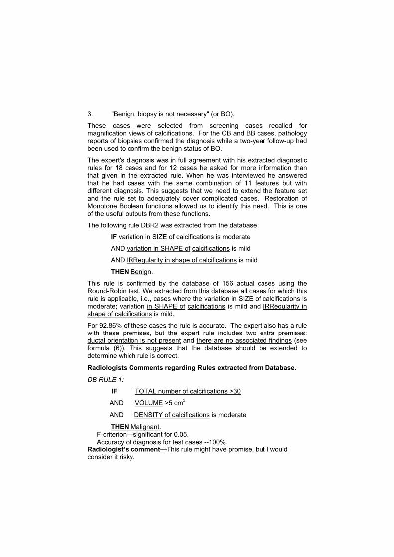
The following rule DBR2 was extracted from the database

IF variation in SIZE of calcifications is moderate

AND variation in SHAPE of calcifications is mild

AND IRRegularity in shape of calcifications is mild

THEN Benign.

This rule is confirmed by the database of 156 actual cases using the Round-Robin test. We extracted from this database all cases for which this rule is applicable, i.e., cases where the variation in SIZE of calcifications is moderate; variation in SHAPE of calcifications is mild and IRRegularity in shape of calcifications is mild.

For 92.86% of these cases the rule is accurate. The expert also has a rule with these premises, but the expert rule includes two extra premises: ductal orientation is not present and there are no associated findings (see formula (6)). This suggests that the database should be extended to determine which rule is correct.

Radiologists Comments regarding Rules extracted from Database.

DB RULE 1:

IF TOTAL number of calcifications >30

AND VOLUME >5 cm3

AND DENSITY of calcifications is moderate

THEN Malignant. F-criterion—significant for 0.05. Accuracy of diagnosis for test cases --100%.

Radiologist’s comment—This rule might have promise, but I would consider it risky.

DB RULE 2:

IF VARIATION in shape of calcifications is marked

AND NUMBER of calcifications is between 10 and 20

AND IRREGULARITY in shape of calcifications is moderate

THEN Malignant. F-criterion—significant for 0.05. Accuracy of diagnosis for test cases -- 100%.

Radiologist’s comment—I would trust this rule.

DB RULE 3:

IF variation in SIZE of calcifications is moderate

AND variation in SHAPE of calcifications is mild

AND IRREGULARITY in shape of calcifications is mild THEN Benign.

F-criterion—significant for 0.05. Accuracy of diagnosis for test cases -- 92.86%.

Radiologist’s comment—I would trust this rule.

6 Discussion The study has demonstrated how consistent and complete data mining in medical diagnosis can acquire a set of logical diagnostic rules for computer-aided diagnostic systems. Consistency avoids contradiction between rules generated using data mining software, rules used by an experienced radiologist, and a database of pathologically confirmed cases.

Two major problems are identified: (1) to find contradiction between diagnostic rules and (2) to eliminate contradiction. Two complimentary intelligent techniques were applied for extraction of rules and recognition of their contradiction.

The first technique is based on discovering statistically significant logical diagnostic rules. The second technique is based on the restoration of a monotone Boolean function to generate a minimal dynamic sequence of questions to a medical expert.

The results of this mutual verification of expert and data-driven rules demonstrate feasibility of the approach for designing consistent breast cancer computer-aided diagnostic systems.

References Abu-Mostafa, Y. 1990. Learning from hints in neural networks. Journal of complexity, 6:192-

198

Alekseev, V. 1988. Monotone Boolean functions. In: Encyclopedia of Mathematics, Vol. 6. Kluwer Academic Publishers, 306-307

[BI-RADS], 1998. Breast Imaging Reporting and Data System. American College of Radiology, Reston, VA

Dedekind, 1897. Rueber Zerlegungen von Zahlen durch ihre grossten gemeinsamen Teiler, Festschrift Hoch. Braunschweig (in German), u.ges. Werke, 103-148

Dhar, V. and Stein, R. 1997. Intelligent Decision Support Methods. Prentice Hall, NJ

CAR’96, 1996. Computer Assisted Radiology. In: Proceedings of the International Symposium on Computer and Communication Systems for Image Guided Diagnosis and Therapy, Eds. Lemke HU, Vannier MW, Inamura K, Farman AG. Paris, France, June 26-29. Elsevier Science, 1996

Craven, M. and Shavlik, J. 1997. Understanding Time-Series Networks: A Case Study in Rule extraction. International Journal of Neural Systems (special issue on Noisy Time Series), 8 (4):374-384

Elmore, J., Wells, M., Carol, M., Lee, H., Howard, D. and Feinstein, A. 1994. Variability in radiologists' interpretation of mammograms. New England Journal of Medicine 331(22): 1493-1449

Fu, Li Min, 1999. Knowledge Discovery Based on Neural Networks. Communications of ACM 42 (11):47-50

Halpern, J.Y. 1990. An analysis of first-order logic of probability. Artificial Intelligence 46: 311-350

Hansel, G. 1966. Sur le nombre des fonctions Boolenes monotones den variables. C.R. Acad. Sci. Paris, 262(20):1088-1090 (in French)

Giarratano, J. and Riley, G. 1994. Expert systems: principles and programming. RWS, Boston

Gurney, J. 1994. Neural Networks at the crossroads: caution ahead. Radiology 193(1): 27-28.

Kleitman, D. 1969. On Dedekind's problem: The number of monotone Boolean functions. In: 5-th Proceedings of the American Mathematics Society 21:677-682

Korobkov, V. 1965. On monotone Boolean functions of algebraic logic. Problemy Cybernetiki 13:5-28. Nauka, Moscow (in Russian)

Kovalerchuk, B. and Lavkov, V. 1984. Retrieval of the maximum upper zero for minimizing the number of attributes in regression analysis. USSR Computational Mathematics and Mathematical Physics 24(4):170-175

Kovalerchuk, B. and Talianski, V. 1992. Comparison of empirical and computed fuzzy values of conjunction. Fuzzy Sets and Systems, 46: 49-53

Kovalerchuk, B., Triantaphyllou, E. and Vityaev, E. 1995. Monotone Boolean functions learning techniques integrated with user interaction. In: Proceedings of the Workshop "Learning from examples vs. programming by demonstration", 12-th International Conference on Machine Learning, Tahoe City. CA, 41-48

Kovalerchuk, B., Triantaphyllou, E., Despande, A. and Vityaev, E. 1996. Interactive Learning of Monotone Boolean Function. Information Sciences, 94 (1-4):87-118

Kovalerchuk, B., Triantaphyllou, E. and Ruiz, J. 1996. Monotonicity and logical analysis of data: a mechanism for evaluation of mammographic and clinical data. In: Kilcoyne RF, Lear JL, Rowberg AH Eds. Computer applications to assist radiology. Carlsbad, CA, Symposia Foundation, 191-196

Kovalerchuk, B., Triantaphyllou, E., Ruiz, J. and Clayton, J. 1997. Fuzzy Logic in Computer-Aided Breast Cancer Diagnosis. Analysis of Lobulation. Artificial Intelligence in Medicine 11:75-85

Kovalerchuk, B., Vityaev, E. and Ruiz, J.F. 1997. Design of consistent system for radiologists to support breast cancer diagnosis. In: Joint Conf. of Information Sciences (Duke University, NC, USA) 2: 118-121

Kovalerchuk, B., Conner, N., Ruiz, J. and Clayton, J. 1998. Fuzzy logic for formalization of breast imaging lexicon and feature extraction. In: 4th Intern. Workshop on Digital Mammography, June 7-10, 1998, University of Nijmegen, Netherlands, http://www.azn.nl/rrng/xray/digmam/iwdm98/Abstracts/node51.html

Kovalerchuk, B. and Vityaev, E. 1998. Discovering Lawlike Regularities in Financial Time Series. Journal of Computational Intelligence in Finance, 6 (3):12-26.

Kovalerchuk B., Vityaev, E. 2000. Data Mining in Finance, Kluwer (in print)

Kovalerchuk, B., Ruiz, J., Vityaev, E. and Fisher, S. 1998. Prototype Internet consultation system for radiologists. Journal of Digital Imaging, 11(3): 22-26, Suppl

Kovalerchuk, B., Vityaev, E. and Ruiz, J. 1999. Consistent knowledge discovery in medical diagnosis. Special issue of the journal: IEEE Engineering in Medicine and Biology Magazine: “Medical Data Mining”.

Krantz, D.H., Luce, R.D., Suppes, P. and Tversky, A. 1971; 1989; 1990; Foundations of Measurement V.1-3. Acad. Press, NY, London

Mitchell, T. 1997. Machine Learning. NY, McCraw Hill

Muggleton, S. 1999. Scientific Knowledge Discovery Using Inductive Logic Programming. Communications of ACM, 42 (11):43-46

Munakata, T. 1999. Knowledge Discovery. Communications of ACM, 42 (11):27-29

Russel, S., Norvig, P. 1995. Artificial Intelligence. A Modern Approach, Prentice Hall

SCAR’96. 1996. Proceedings of the Symposium for Computer Applications in Radiology. Eds. Kilcoyne RF, Lear JL, Rowberg AH Computer applications to assist radiology. Carlsbad, CA, Symposia Foundation

SCAR’98. 1998. Proceedings of the Symposium for Computer Applications in Radiology. Journal of Digital Imaging 11(3), Suppl

Shavlik, J.W. 1994. Combining symbolic and neural learning. Machine Learning, 14:321-331

Shtern, F. 1996. Novel digital technologies for improved control of breast cancer. In: CAR’96, Computer Assisted Radiology, Proceedings of the International Symposium on Computer and Communication Systems for Image Guided Diagnosis and Therapy, Lemke, H.U., Vannier, M.W., Elsevier, pp.357-361

TIWDM. 1996. Third International Workshop on Digital Mammography. University of Chicago, Chicago, IL, Abstracts, June 9-12, 1996

TIWDM. 1998. 4th Intern. Workshop on Digital Mammography, June 7-10, 1998. University of Nijmegen, Netherlands, 1998, http://www.azn.nl/rrng/xray/digmam/iwdm98/Abstracts/node51.html

Vityaev, E.E. 1992. Semantic approach to knowledge base development. Semantic probabilistic inference. Computational Systems, 146: 19-49, Novosibirsk (in Russian)

Vityaev, E.E. and Moskvitin, A.A. 1993. Introduction to discovery theory: Discovery software system. Computational Systems, 148: 117-163, Novosibirsk (in Russian)

Vityaev, E.E. and Logvinenko, A.D. 1998. Laws discovery on empirical systems. Axiom systems of measurement theory testing. Sociology: methodology, methods, mathematical models (Scientific journal of Russian Academy of Science) 10:97-121 (in Russian)

Wingo, P.A., Tong, T. and Bolden, S. 1995. Cancer statistics. Ca-A Cancer Journal for Clinicians, 45(1): 8-30.