Considerations and Techniques for Analyzing Domains of Complex

1

Paper 449-2013

Considerations and Techniques for Analyzing Domains of

Complex Survey Data

Taylor Lewis1, U.S. Office of Personnel Management, Washington, DC, USA

ABSTRACT

Despite sounding like a straightforward task, making inferences on a domain, or subset, of a complex survey data set is something that is often done incorrectly. After briefly discussing the features constituting “complex” survey data, this paper explains the risks behind simply filtering the full data set for cases in the domain of interest prior to running a SAS/STAT® SURVEY procedure such as PROC SURVEYMEANS or PROC SURVEYREG. Instead, it will be shown how one should use the DOMAIN statement or create a domain-specific analysis weight. Also discussed in detail are considerations and approaches to the very common objective of testing whether the difference between two domain means is statistically significant.

BACKGROUND ON FEATURES OF COMPLEX SURVEY DATA

This paper begins with a discussion of what constitutes “complex” survey data. Specifically, there are four distinct features that can arise:

Finite population corrections

Clustering

Stratification

Unequal weights

In general, if the data emanate from a sample design that introduced one or more of these features, you should employ a SAS/STAT analysis procedure prefixed by SURVEY. There are currently five such procedures:

PROC SURVEYMEANS

PROC SURVEYFREQ

PROC SURVEYREG

PROC SURVEYLOGISTIC

PROC SURVEYPHREG

All five share a common syntax structure to inform SAS® of these features in the input data set.

In many introductory statistics courses, the implied data collection mechanism is simple random sampling with replacement, possibly from an infinite or hypothetical population. Under that paradigm, data are assumed independently and identically distributed, or i.i.d. for short. In contrast, survey researchers often select samples without replacement from finite, or enumerable, populations, and simple random sampling is the exception rather than the rule. Alternative sample designs can yield efficiencies in many circumstances, but they are most often pursued out of necessity or to save on data collection costs.

For sake of an example, assume a state board of education is interested in measuring the mathematical aptitude of N = 1,000 students at a particular high school by way of a standardized test. That is, the finite population of interest is the student body of the given school. Instead of administering the test to all students, suppose a sample of n = 200 students is selected randomly and that an aptitude yi is measured for each. We know from standard statistical theory

that the sample mean is n

y

y

n

i

i 1ˆ an unbiased estimate of y , the true population mean, or the average test score

for all students in the high school. If the sample were selected with replacement, meaning each student in the population could be sampled (and measured via the test) more than once, the estimated variance of the sample

1 The opinions, findings, and conclusions expressed in this article are those of the authors and do not necessarily

reflect those of the U.S. Office of Personnel Management.

Statistics and Data AnalysisSAS Global Forum 2013

Considerations and Techniques for Analyzing Domains of Complex Survey Data, continued

2

mean would be calculated as

)(

ˆ

)ˆv ar(1

1 1

2

n

yy

ny

n

i

i

. If the sample were selected without replacement, however,

the variance formula would be modified to

N

n

n

yy

ny

n

i

i

11

1 1

2

)(

ˆ

)ˆv ar( . In other words, sampling without

replacement reduces the variance in proportion to the sampling rate—in this case, 20%.

The term (1 – n/N) is called the finite population correction, or FPC, and enters other estimators’ variance formulas, not strictly that of the sample mean. Notice that as the sampling fraction approaches 1, the variance tends to 0, which is an intuitive result. Another way of conceptualizing this is that, as the portion of the population sampled increases, uncertainty in a sample-based estimate decreases. In the most extreme case of a census (when n = N), the FPC is 0 and there is no variance. The sample-based estimate defaults to the given population quantity.

One straightforward way to incorporate the FPC is to use the TOTAL= option in the PROC statement. SAS determines the sample size, n, from the input data set, but relies on the user to specify the population size, N. Alternatively, you can specify the sampling rate, n/N, using the RATE= option. If neither the TOTAL= or RATE= options is present, the SURVEY procedure assumes sampling was conducted with replacement and ignores the FPC.

The second feature is clustering, which occurs when the unit sampled is actually a cluster of population units.

Returning to our hypothetical example, suppose that each student in the high school starts his or her school day in a homeroom where attendance is taken and other administrative matters handled. For numeric concreteness, assume there are 40 homerooms, each comprised of 25 students. From the standpoint of data collection logistics, it would be much easier to sample homerooms and administer the test therein as opposed to tracking down each sampled student independently. One could still achieve a sample size of 200 by sampling 8 of the 40 homerooms. This is a legitimate sample design, but the clustering should be accounted in the analysis stage by specifying a homeroom identifier variable in the CLUSTER statement of the respective SURVEY procedure.

There is no mandate to sample all units within a cluster. For instance, we could have achieved the same sample size by initially selecting 20 homerooms, then selecting 10 students from each at random. This is an example of a multi-stage sampling design in which the primary sampling units (PSUs) are homerooms and the secondary sampling units (SSUs) are students. It is worth emphasizing, however, that only the PSU identifier should be specified in the CLUSTER statement. When SAS sees two variables in the CLUSTER statement, it assumes the combination of the two defines a PSU, which can result in an unduly low variance estimate. Specifying only the PSU implicitly invokes the ultimate cluster assumption (p. 67 of Heeringa et al., 2010) that is frequently used to simplify variance calculations. A common concern voiced by practitioners is that this does not account for all stages of sampling and, thus, may underestimate variability. More commonly, however, the result is a slight overestimation of variability

2.

The third feature of complex survey data is stratification, which arises when PSUs are allocated into one of a mutually exclusive and exhaustive set of groups, or strata (singular: stratum) and an independent sample is selected within each. Whereas clustering typically decreases precision, in all but a few rare circumstances, stratification increases precision. The reason is that the overall variance consists of stratum-specific variance estimates summed over all strata. When strata are constructed homogeneously with respect to the principle outcome variable(s), there can be considerable precision gains relative to simple random sampling.

Returning to our hypothetical example, a prudent stratification variable might be grade level. Suppose the 40 homerooms could be grouped into 4 sets of 10, one for each grade level—ninth through twelfth. Figure 1 illustrates how this might look if 2 homerooms were sampled within each grade. Rows correspond to strata, columns to clusters, and a filled-in cell denotes being selected into the sample. If this particular sample design was employed, however, we would need to inform SAS of the grade level identifier by placing it in the STRATA statement of the given SURVEY procedure.

2 For a few empirical discussions drawn from surveys using multi-stage sampling approaches, see

http://www.isr.umich.edu/src/smp/asda/first_stage_ve_new.pdf or

http://www.cdc.gov/nchs/data/ahcd/ultimatecluster.pdf.


http://www.isr.umich.edu/src/smp/asda/first_stage_ve_new.pdf

http://www.cdc.gov/nchs/data/ahcd/ultimatecluster.pdf


3

Homeroom

1 2 3 4 5 6 7 8 9 10

Grade

9

10

11

12

Figure 1. Visual Representation of a Stratified, Cluster Sample for the Hypothetical Mathematics Aptitude Survey

Parenthetically alluded to above was how sampling rates of clusters may vary across strata. In general, when sampling rates vary amongst the ultimately sampled units, one should account for this by assigning a unit-level weight equaling the inverse of that unit’s selection probability. Weights are the fourth feature of complex survey data and can be interpreted as the number of population units a sample unit represents. For instance, if a sample unit’s selection probability was one-fourth, that unit would be assigned a weight of 4. The unit’s survey responses represent itself and three other comparable units in the population. Where applicable, these weights should be stored as a numeric weight variable and specified in the WEIGHT statement of the SURVEY procedure. In the absence of a WEIGHT statement, units are implicitly assigned a weight of 1.

DEFINITION OF DOMAIN ESTIMATION

Domain estimation is the term referring to an analysis focused on only a portion of the target population. Continuing with our hypothetical mathematics aptitude survey, computing the mean test score using the entire data set is tantamount to making inferences on the entire high school. Certainly this is an objective of the survey campaign, but we might also like to make comparisons such as ninth grade versus tenth grade, males versus females, etc. It is tempting to simply filter out from the data set units residing in the domain of interest (e.g., females) or put the domain identifier in a BY statement, then proceed with a SURVEY procedure to obtain the desired domain-specific statistics and measures of variability. This is risky, however, as it can lead one to make erroneous inferences depending on the nature of the domain.

Generally speaking, the only harmless occasion to subset the data set is when the domain of interest is a proper subset, meaning it is comprised of all units in one or more strata. In terms of our hypothetical survey, this means we

are free to subset the data set for cases in a particular grade or combinations of grade. Figure 2 depicts two proper subset examples, an analysis restricted to tenth grade students and an analysis restricted to upperclassmen.

Homeroom

1 2 3 4 5 6 7 8 9 10

Grade

9

10

11

12

Homeroom

1 2 3 4 5 6 7 8 9 10

Grade

9

10

11

12

Figure 2. Two Examples of Proper Subsets in the Hypothetical Mathematics Aptitude Survey: Tenth Grade Students (above) and Upperclassmen (below)

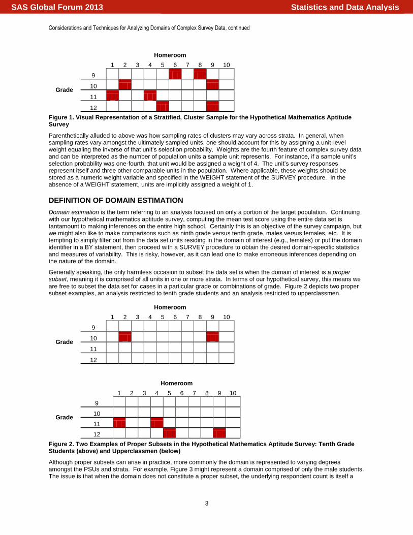
Although proper subsets can arise in practice, more commonly the domain is represented to varying degrees amongst the PSUs and strata. For example, Figure 3 might represent a domain comprised of only the male students. The issue is that when the domain does not constitute a proper subset, the underlying respondent count is itself a



4

random variable and this additional uncertainty should be reflected. One built-in method is to specify the domain identifier variable(s) in the DOMAIN statement, available in every SURVEY procedure. As we will see, point estimates from output generated from the DOMAIN statement match point estimates generated from subsetting, but measures of variability and degrees of freedom are not necessarily equivalent.

Homeroom

1 2 3 4 5 6 7 8 9 10

Grade

9

10

11

12

Figure 3. Visual Representation of a General Domain Analysis (e.g., Gender) in the Hypothetical Mathematics Aptitude Survey

A REAL-WORLD COMPLEX SURVEY: THE NATIONAL AMBULATORY MEDICAL CARE SURVEY (NAMCS)

The fictitious mathematics aptitude survey was introduced to facilitate exposition of the particular complex survey features data analysts may encounter and the concept of domain estimation. We now shift attention to a real-world complex survey, the National Ambulatory Medical Care Survey (NAMCS). Sponsored by the National Center for Health Statistics (NCHS), a Federal Statistical Agency within the Centers for Disease Control and Prevention (CDC), NAMCS collects data on outpatient visits to non-emergency physician’s offices. That is, the ultimate sample unit is a physician visit. Examples of variables measured by the survey include diagnoses made, chronic illnesses of the patient, time spent with the physician, and medications prescribed or renewed. NCHS administers NAMCS on a yearly basis, and in addition to various tabulations and publications, NCHS releases data via a public-use microdata file. Instructions on how to download the data can be found on their website: http://www.cdc.gov/nchs/ahcd.htm. In this paper, we will highlight analyses using the 2009 NAMCS public-use data set.

A wise first step to understand the design elements and complex features of a survey is to consult any user documentation available. According to the documentation (available on-line at: ftp://ftp.cdc.gov/pub/Health_Statistics/NCHS/Dataset_Documentation/NAMCS/doc09.pdf), NAMCS has three of the features discussed in the previous section:

1. Stratification – strata are identified by distinct codes of the CSTRATM variable.

2. Clustering – each PSU is identified (within a stratum) by distinct codes of CPSUM.

3. Unequal Weighting – weights can be specified by the PATWT variable.

The NAMCS public-use file contains hundreds of variables. Aside from the key design variables noted above, Table 1 summarizes the manageable subset of these variables that will be used in this paper.

Table 1. Summary of NAMCS 2009 Public-Use Data Set Variables Used in this Paper

Variable Name Description Coding Structure

SEX Patient Gender 1 = Female 2 = Male

AGE Patient Age in Years Continuous

SOLO Indicator of Solo Physician Practice 1 = Yes 2 = No

MED Indicator of Medication Prescribed 0 = No 1 = Yes

TIMEMD Time Spent with Physician in Minutes Continuous, ranging from 0 to 240

MAJOR Primary Reason for Visit 1 = New problem (<3 mos. onset) 2 = Chronic problem, routine 3 = Chronic problem, flare up 4 = Pre-/Post-surgery 5 = Preventive care (e.g. routine prenatal, well-baby, screening, insurance, general exams)



5

MRI Indicator of whether an MRI was Ordered 1 = Yes 0 = No

WHY SUBSETTING IS RISKY

To illustrate the risk behind subsetting the full survey data set, suppose one was interested in estimating the mean time spent with the physician (TIMEMD) for visits during which an MRI was ordered. In the example syntax below, two methods are used. The first subsets the full data set for cases of interest (those where MRI=1), while in the second the MRI variable is specified in the DOMAIN statement. The output generated by these two PROC SURVEYMEANS runs immediately follows. Note that when a DOMAIN statement is used the SURVEY procedure conducts an overall analysis followed by a series of domain-specific analyses based on every unique, non-missing value of the variable(s) identified. (Domains can also be defined based on the combination of two or more variables’ values—syntax follows that used in the TABLE statement of PROC FREQ.)

*** demonstrating two methods of domain analysis for mean time spent with physician

when an MRI was ordered;

* 1) subsetting;

proc surveymeans data=NAMCS_2009 nobs mean stderr;

where MRI=1;

stratum CSTRATM;

cluster CPSUM;

var TIMEMD;

weight PATWT;

run;

* 2) using the DOMAIN statement;


stratum CSTRATM;

cluster CPSUM;

var TIMEMD;

weight PATWT;

domain MRI;

run;

The SURVEYMEANS Procedure

Data Summary

Number of Strata 48

Number of Clusters 166

Number of Observations 658

Sum of Weights 16841215

Statistics

Std Error

Variable N Mean of Mean

ƒƒƒƒƒƒƒƒƒƒƒƒƒƒƒƒƒƒƒƒƒƒƒƒƒƒƒƒƒƒƒƒƒƒƒƒƒƒƒƒƒƒƒƒƒƒƒƒƒƒƒƒƒƒƒƒ

TIMEMD 658 23.415071 1.633407




6


Data Summary

Number of Strata 70

Number of Clusters 617

Number of Observations 32281

Sum of Weights 1037796486

Statistics

Std Error



TIMEMD 32281 19.586527 0.271539


Domain Analysis: MRI

Std Error

MRI Variable N Mean of Mean

ƒƒƒƒƒƒƒƒƒƒƒƒƒƒƒƒƒƒƒƒƒƒƒƒƒƒƒƒƒƒƒƒƒƒƒƒƒƒƒƒƒƒƒƒƒƒƒƒƒƒƒƒƒƒƒƒƒƒƒƒƒƒƒƒ

0 TIMEMD 31623 19.523373 0.267039

1 TIMEMD 658 23.415071 1.684196

ƒƒƒƒƒƒƒƒƒƒƒƒƒƒƒƒƒƒƒƒƒƒƒƒƒƒƒƒƒƒƒƒƒƒƒƒƒƒƒƒƒƒƒƒƒƒƒƒƒƒƒƒƒƒƒƒƒƒƒƒƒƒƒƒ

From the output above, we observe the point estimates are equivalent (23.415) for either method, but the standard error is larger when the DOMAIN statement is used—1.684 versus 1.633. The discrepancy is caused by the fact that the MRI=1 condition does not occur in all PSUs. This can be gathered by comparing the two Data Summary components of the output. SAS is only aware of the distinct stratum and PSU codes for cases that meet the WHERE statement condition, and the problem is that there are certain strata in which all such cases come from a single PSU. By default, there must be at least two PSUs in a given stratum for variance calculation purposes. When only one is detected, the procedure still runs, but the following message is output to the log:

NOTE: Only one cluster in a stratum for variable(s) TIMEMD. The estimate of variance for TIMEMD

will omit this stratum.

SAS is alerting you that the overall variance estimate is ignoring one or more strata. Since the overall variance estimate is the summation of stratum-specific variances, all of which are greater than or equal to zero, this necessarily leads to a variance underestimation. For these reasons, it is advised never to subset the data prior to invoking a SURVEY procedure.

TESTING WHETHER DOMAIN MEAN DIFFERENCES ARE SIGNIFICANT

After estimating the domain means and their measures of variability properly, a natural next step is testing whether the observed difference between two domain means is statistically significant. Continuing with the NAMCS example, we might be interested in assessing whether having an MRI ordered during the physician visit is associated with more time spent with the physician than not having one ordered. In terms of formal statistical hypotheses, this is like

testing H0: 01 MRIMRI yy versus H1: 01 MRIMRI yy .

Analysts often proceed with this kind of test implicitly assuming the two estimates are independent. That is, they compute a t-statistic such as

)ˆv ar()ˆv ar(

ˆˆ

01

01

MRIMRI

MRIMRI

yy

yyt



7

where )ˆv ar( 1MRIy is the squared standard error (i.e., variance) for the sample mean of the MRI cases and

)ˆv ar( 0MRIy is the like for non-MRI cases. In actuality, the independence assumption only applies when the two

domains constitute non-overlapping proper subsets. On the other hand, when the two domain estimates are drawn from a shared set of PSUs, there is generally a non-zero covariance between the two sample mean estimates. If so, the variance of the difference—what appears in the denominator of the t-test above—is no longer simply the sum of

the two underlying variances, but rather )ˆ,ˆcov ()ˆvar()ˆvar( 0101 2 MRIMRIMRIMRI yyyy .

There is currently no way to conduct t-tests on domain mean differences within PROC SURVEYMEANS itself. If the two domains happen to be disjoint proper subsets, you could use ODS statements to store the Domain Analysis portion of the output in a separate data set that can be further manipulated. Another option with the same net effect would be to utilize the CONTRAST= parameter in the %SMSUB macro

3 (requires SAS/IML). Neither of these options

can account for a non-zero covariance between two domain means, however.

An alternative method for conducting domain mean significance tests is to use PROC SURVEYREG. The general method is as follows. First, create a 0/1 indicator variable in the raw data to distinguish the two domains. Next, fit a simple linear regression model on the outcome variable of interest with this indicator variable serving as the lone predictor. It can be shown that the t-statistic generated from the null hypothesis that the slope coefficient in this simple model is zero is algebraically equivalent to the (two-tailed) two-sample t-test statistic shown above. The

technique works for either proper subsets or domains drawn from a shared set of PSUs.

The syntax below demonstrates this approach by testing whether the mean time spent with the physician is significantly longer when an MRI is ordered. The MRI variable from the example above conveniently conforms to the 0/1 pattern, so no additional recoding is necessary. The only other option deserving mention is VADJUST=NONE appearing after the slash in the MODEL statement. This overrides a default variance-covariance matrix adjustment factor PROC SURVEYREG uses based on the small sample bias noted by Hidiroglou et al. (1980). The factor is (n – 1)/(n – p), where n is the number of observations in the data set and p is the number of model parameters including the intercept. So when n >> p, the adjustment factor converges to 1. Overriding the default ensures conclusions from the slope coefficient test in PROC SURVEYREG mirror precisely conclusions from a two-sample t-test performed independently.

* demonstrating how to use PROC SURVEYREG to test whether two domain means are

significantly different from one another;

proc surveyreg data=NAMCS_2009;

stratum CSTRATM;

cluster CPSUM;

model TIMEMD = MRI / vadjust=none;

weight PATWT;

run;

Estimated Regression Coefficients

Standard

Parameter Estimate Error t Value Pr > |t|

Intercept 19.5233733 0.26703936 73.11 <.0001

MRI 3.8916974 1.62666409 2.39 0.0171

Comparing the output here with the PROC SURVEYMEANS output presented earlier—where MRI appeared in the DOMAIN statement—one can verify that the parameter estimate (i.e., slope coefficient) for the MRI variable is simply the difference in domain means (3.8917 = 23.4151 – 19.5234). We can reason the covariance must be accounted for in the standard error, because the independence assumption would have led to a value of

7052.12670.06842.1 22 . We can further reason the covariance must have been positive, since the reported

standard error is slightly smaller at 1.6267. Hence, abandoning the independence assumption is beneficial in this case as it fosters more statistical power, or increases the likelihood of concluding a statistically significant difference. Indeed, examining what is reported in the “t Value” column and its corresponding p-value, we might conclude the observed difference is significant, at least at the α=.05 level.

3 http://support.sas.com/kb/25/033.html


http://support.sas.com/kb/25/033.html


8

While the technique is straightforward, it would be tedious to conduct on multiple domain mean differences. Suppose a particular domain-defining variable is comprised of D unique levels. To calculate all distinct D(D – 1)/2 mean significance tests, we would need to code in as many 0/1 indicator variables and as many MODEL statements. A feature new to PROC SURVEYREG as of Version 9.22 greatly reduces the amount of syntax required.

Staying with NAMCS, suppose that instead of a simple dichotomous indicator of whether an MRI was ordered, we were interested in contrasting mean time spent with the physician based on the primary reason for the visit (MAJOR). Table 1 lists five possible categorizations for this variable:

1. New problem (<3 mos. onset)

2. Chronic problem, routine

3. Chronic problem, flare up

4. Pre-/Post-surgery

5. Preventive care (e.g. routine prenatal, well-baby, screening, insurance, general exams)

This can be accomplished by putting MAJOR, the domain identifier variable, in the CLASS statement as well as the sole predictor variable to the right of the equals sign in the MODEL statement, and also specifying this variable in the LSMEANS statement with the DIFF option provided after the slash. Only the two pertinent components of the output generated are shown here. The first is a summarization of the marginal means and standard errors, with default tests of significance assessing whether each is significantly different from zero. The second is a list of all 5(5 – 1)/2 = 10 unique mean differences that can be formed using the 5 categorizations of MAJOR.

* illustrating the new LSMEANS statement in PROC SURVEYREG;


stratum CSTRATM;

cluster CPSUM;

class MAJOR;

model TIMEMD = MAJOR / vadjust=none;

weight PATWT;

lsmeans MAJOR / diff;

run;

MAJOR Least Squares Means

Standard

MAJOR Estimate Error DF t Value Pr > |t|

1 18.8177 0.3405 546 55.27 <.0001

2 19.8661 0.3951 546 50.28 <.0001

3 22.0707 0.6069 546 36.37 <.0001

4 18.2587 0.5111 546 35.72 <.0001

5 20.0038 0.5180 546 38.62 <.0001

Differences of MAJOR Least Squares Means

Standard

MAJOR _MAJOR Estimate Error DF t Value Pr > |t|

1 2 -1.0484 0.4488 546 -2.34 0.0199

1 3 -3.2530 0.6306 546 -5.16 <.0001

1 4 0.5590 0.5503 546 1.02 0.3102

1 5 -1.1861 0.5121 546 -2.32 0.0209

2 3 -2.2046 0.6821 546 -3.23 0.0013

2 4 1.6074 0.6401 546 2.51 0.0123

2 5 -0.1378 0.5765 546 -0.24 0.8112

3 4 3.8120 0.8353 546 4.56 <.0001

3 5 2.0669 0.7832 546 2.64 0.0086

4 5 -1.7451 0.5838 546 -2.99 0.0029



9

A few additional options available after the slash in the LSMEANS statement deserve brief mention:

The significance level for the pairwise tests can be modified using the ALPHA= option.

Related to the point above, there are a variety of p-value adjustment techniques available within the ADJUST= option. These are aimed at controlling the overall Type I error rate, many of which also appear in PROC MULTTEST—for more background on these procedures, see the documentation.

The PLOTS= option offers a suite of pre-configured ODS Graphics-based visualizations that could prove useful for deciphering underlying patterns.

Another point worth emphasizing before moving on to the next topic is that the PROC SURVEYREG approaches demonstrated in this section translate to dichotomous outcome variables so long as the two categories are coded one unit apart (e.g., a 0/1 indicator variable). For example, we might be interested in contrasting the probability a medication is prescribed during the visit among the various primary reasons for the visit—the variable MED is a numeric 0/1 indicator of this event occurring. To conduct this analysis, we could simply swap MED for TIMEMD in the code above. This is not an endorsement for the application of linear regression on a dichotomous outcome variable—logistic regression would be the preferred approach, for reasons Hosmer and Lemeshow (2000) make poignantly clear in their opening chapter—but the algebraic equivalence relative to two-sample t-tests is maintained for proportions just as it is for means of continuous outcome variables.

DOMAIN ESTIMATION IN LINEAR MODELS

All of the same principles and problems outlined above apply to any of the SURVEY procedures that fit linear models. For example, suppose one was interested in modeling time spent with the physician as a function of the primary reason for the visit, while simultaneously accounting for effects of patient age (AGE) and gender (SEX). Moreover, suppose the goal was to evaluate these relationships only for visits to a physician who practice alone—defined by SOLO=1.

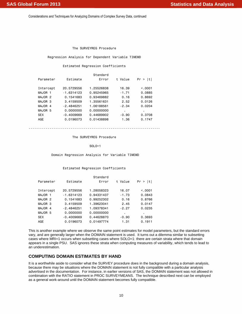
The syntax below performs this analysis by fleshing out some the PROC SURVEYREG syntax used in the previous section. In addition to MAJOR, AGE and SEX are added to the MODEL statement. Although SEX is a categorical variable, males and females are coded one unit apart, so it does not technically need to be placed in the CLASS statement. Since a CLASS statement is used for MAJOR, however, the option SOLUTION after the slash in the model statement is required to have the weighted least squares model parameter estimates output to this listing. The first SURVEYREG run subsets data for cases in the domain of interest, while the second run (properly) places the SOLO variable in the DOMAIN statement. For brevity, only select output from each SURVEYREG run is shown.

*** demonstrating a domain analysis for a linear regression model;

* 1) subsetting;


where SOLO=1;

stratum CSTRATM;

cluster CPSUM;

class MAJOR;

model TIMEMD = MAJOR SEX AGE / vadjust=none solution;

weight PATWT;

run;

* 2) using the DOMAIN statement;


stratum CSTRATM;

cluster CPSUM;

class MAJOR;

model TIMEMD = MAJOR SEX AGE / vadjust=none solution;

weight PATWT;

domain SOLO;

run;



10

The SURVEYREG Procedure

Regression Analysis for Dependent Variable TIMEMD


Standard


Intercept 20.5729556 1.25526838 16.39 <.0001

MAJOR 1 -1.6314123 0.95245965 -1.71 0.0885

MAJOR 2 0.1541683 0.93469882 0.16 0.8692

MAJOR 3 3.4159509 1.35561631 2.52 0.0126

MAJOR 4 -2.4846251 1.06188561 -2.34 0.0204

MAJOR 5 0.0000000 0.00000000 . .

SEX -0.4009669 0.44689902 -0.90 0.3708

AGE 0.0196073 0.01438898 1.36 0.1747

---------------------------------------------------------------------

The SURVEYREG Procedure

SOLO=1

Domain Regression Analysis for Variable TIMEMD


Standard


Intercept 20.5729556 1.28058323 16.07 <.0001

MAJOR 1 -1.6314123 0.94331437 -1.73 0.0843

MAJOR 2 0.1541683 0.99252302 0.16 0.8766

MAJOR 3 3.4159509 1.39623041 2.45 0.0147

MAJOR 4 -2.4846251 1.09378341 -2.27 0.0235

MAJOR 5 0.0000000 0.00000000 . .

SEX -0.4009669 0.44628870 -0.90 0.3693

AGE 0.0196073 0.01497774 1.31 0.1911

This is another example where we observe the same point estimates for model parameters, but the standard errors vary, and are generally larger when the DOMAIN statement is used. It turns out a dilemma similar to subsetting cases where MRI=1 occurs when subsetting cases where SOLO=1: there are certain strata where that domain appears in a single PSU. SAS ignores these strata when computing measures of variability, which tends to lead to an underestimation.

COMPUTING DOMAIN ESTIMATES BY HAND

It is a worthwhile aside to consider what the SURVEY procedure does in the background during a domain analysis, because there may be situations where the DOMAIN statement is not fully compatible with a particular analysis advertised in the documentation. For instance, in earlier versions of SAS, the DOMAIN statement was not allowed in combination with the RATIO statement in PROC SURVEYMEANS. The technique described next can be employed as a general work-around until the DOMAIN statement becomes fully compatible.



11

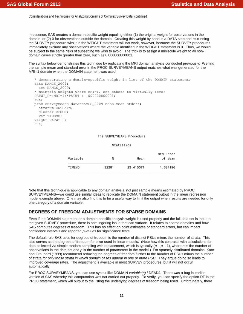
In essence, SAS creates a domain-specific weight equaling either (1) the original weight for observations in the domain, or (2) 0 for observations outside the domain. Creating this weight by hand in a DATA step and re-running the SURVEY procedure with it in the WEIGHT statement will not work, however, because the SURVEY procedures immediately exclude any observations where the variable identified in the WEIGHT statement is 0. Thus, we would be subject to the same risks of subsetting we wish to avoid. The trick is to assign a miniscule weight to all non-domain cases strictly greater than zero, such as 0.000000000001. The syntax below demonstrates this technique by replicating the MRI domain analysis conducted previously. We find the sample mean and standard error in the PROC SURVEYMEANS output matches what was generated for the MRI=1 domain when the DOMAIN statement was used.

* demonstrating a domain-specific weight in lieu of the DOMAIN statement;

data NAMCS_2009;

set NAMCS_2009;

* maintain weights where MRI=1, set others to virtually zero;

PATWT_D=(MRI=1)*PATWT + .000000000001;

run;


stratum CSTRATM;

cluster CPSUM;

var TIMEMD;

weight PATWT_D;

run;


Statistics

Std Error



TIMEMD 32281 23.415071 1.684196


Note that this technique is applicable to any domain analysis, not just sample means estimated by PROC SURVEYMEANS—we could use similar ideas to replicate the DOMAIN statement output in the linear regression model example above. One may also find this to be a useful way to limit the output when results are needed for only one category of a domain variable.

DEGREES OF FREEDOM ADJUSTMENTS FOR SPARSE DOMAINS

Even if the DOMAIN statement or a domain-specific analysis weight is used properly and the full data set is input to the given SURVEY procedure, there is one lingering issue that can surface. It relates to sparse domains and how SAS computes degrees of freedom. This has no effect on point estimates or standard errors, but can impact confidence intervals and reported p-values for significance tests.

The default rule SAS uses for degrees of freedom is the number of distinct PSUs minus the number of strata. This also serves as the degrees of freedom for error used in linear models. (Note how this contrasts with calculations for data collected via simple random sampling with replacement, which is typically (n – p – 1), where n is the number of observations in the data set and p is the number of parameters in the model.) For sparsely distributed domains, Korn and Graubard (1999) recommend reducing the degrees of freedom further to the number of PSUs minus the number of strata for only those strata in which domain cases appear in one or more PSU. They argue doing so leads to

improved coverage rates. The adjustment is available in most SURVEY procedures, but it will not occur automatically.

For PROC SURVEYMEANS, you can use syntax like DOMAIN variable(s) / DFADJ. There was a bug in earlier version of SAS whereby this computation was not carried out properly. To verify, you can specify the option DF in the PROC statement, which will output to the listing the underlying degrees of freedom being used. Unfortunately, there



12

is no way to hardwire the degrees of freedom employed by PROC SURVEYMEANS. In PROC SURVEYREG, however, you can simply specify DF=integer after the slash in the MODEL statement.

CONCLUSION

This paper began with a discussion of the four features that may appear in a complex survey data set: finite population corrections, clustering, stratification, and unequal weights. In general, when analyzing data of this sort, one should employ one of the five SAS/STAT procedures prefixed by SURVEY. Using examples drawn from the National Ambulatory Medical Care Survey, it has been emphasized that when one is interested in analyzing only a portion of the data to make inferences on a domain of the target population, one should utilize the DOMAIN statement—available in all SURVEY procedures—or create a domain-specific analysis weight. Despite an analyst’s instinct to simply subset the data set, there is a significant risk such an approach can lead to flawed measures of variability.

The paper also discussed in detail the common task of testing whether the difference between two domain sample means is significant. The new LSMEANS statement in PROC SURVEYREG offers a flexible way to conduct these tests, even if the variable is dichotomous or a non-zero covariance exists between the estimates. Readers were also alerted of the degrees of freedom reduction recommended by Korn and Graubard (1999) when the domain of interest does not appear in all strata.

In closing, it should be acknowledged that the hazards identified here are only applicable when one uses the default variance approximation technique, Taylor series linearization. An increasingly popular class of alternatives is replication variance approximation methods. These methods have been around for many years, and became available in SAS with the release of version 9.2. A good reference with more detail and syntax examples is Mukhopadhyay et al. (2008).

Replication approaches are typically operationalized by appending a set of replicate weights to the analysis file. The idea is to compute the given estimate using the full-sample weight and repeat using each of the replicate weights. The variability of the full-sample estimate is a function of the replicate weight estimates’ squared deviations about the full-sample estimate. An appeal of these approaches is that there is generally a single variance formula per method, regardless of the quantity. Since the replicate weights contain all the pertinent sample design information, however, subsetting is permitted for domain analyses. These methods also abide by different degrees of freedom rules, but they will not be discussed further in this paper.

REFERENCES

Heeringa, S., West, B., and Berglund, P. (2010). Applied Survey Data Analysis. Boca Raton, FL: Chapman & Hall.

Hidiroglou, M., Fuller, W., and Hickman, R.. (1980). SUPER CARP, Ames: Statistical Laboratory, Iowa State

University.

Hosmer, D., and Lemeshow, S. (2000). Applied Logistic Regression. Second Edition. New York, NY: Wiley.

Korn, E., and Graubard, B. (1999). Analysis of Health Surveys. New York, NY: Wiley.

Mukhopadhyay, P., An, A., Tobias, R., and Watts, D. (2008). “Try, Try Again: Replication-Based Variance Estimation Methods for Survey Data Analysis in SAS® 9.2,” Proceedings of the SAS Global Forum Conference. San Antonio, TX, March 16 – 19. Retrieved October 3, 2012 at: http://www2.sas.com/proceedings/forum2008/367-2008.pdf

CONTACT INFORMATION

Your comments and questions are valued and encouraged. Contact the author at:

Name: Taylor Lewis Enterprise: U.S. Office of Personnel Management Address: 1900 E St., NW City, State ZIP: Washington, DC 20415 E-mail: [email protected]

SAS and all other SAS Institute Inc. product or service names are registered trademarks or trademarks of SAS Institute Inc. in the USA and other countries. ® indicates USA registration.

Other brand and product names are trademarks of their respective companies.


http://www2.sas.com/proceedings/forum2008/367-2008.pdf

mailto:[email protected]

Documents

Considerations and Techniques for Analyzing Domains of Complex