Embed Size (px)
Citation preview
Conservation Reserve ProgramCP33 - Habitat Buffers for Upland Birds
2006 Annual Report
Bird Monitoring and Evaluation Plan
FWRC
Conservation Reserve ProgramBird Monitoring and Evaluation Plan
2006 Annual Report
Kristine O. EvansResearch Associate II
Department of Wildlife and Fisheries, Mississippi State University
Wes BurgerProfessor of Wildlife Ecology
Department of Wildlife and Fisheries, Mississippi State University
Mark D. SmithPostdoctoral Associate
Department of Wildlife and Fisheries, Mississippi State University
Sam RiffellAssistant Professor
Department of Wildlife and Fisheries, Mississippi State University

Executive SummaryIn 2005, the USDA-Farm Service Agency (FSA) implemented the Habitat Buffers for Upland Birds (CP33)
practice as part of the Continuous Conservation Reserve Program (CRP). The FSA allocated 250,000 CP33 acres
to 35 states to be actively managed over a period of 10 years and charged the Southeast Quail Study Group with
the development of a CP33 monitoring protocol with the goal of generating measures of population response for
northern bobwhite (Colinus virginianus) and other priority songbird species.
The FSA adopted the monitoring protocol developed by the SEQSG and encouraged states with CP33
allocation to participate in coordinated monitoring. The CP33 national monitoring protocol suggested monitoring
of the 20 states that encompass 95% of the allocated CP33 acreage over a 3 year period. State-level point-transect
monitoring began in the 2006 breeding season on at least 40 CP33 contract fields paired with similarly cropped
control fields in 11 states. Monitoring continued in the fall of 2006 with bobwhite covey call surveys in 14 states.
Comparative abundance of bobwhite and other priority species on CP33 and control fields were estimated for
the 2006 breeding season and fall using a 3-tiered approach (across bobwhite range (national), within each Bird
Conservation Region (BCR), and within each state).
There was a positive overall response by bobwhite and variable response by priority songbird species to
establishment of CP33 habitat buffers around cropped fields compared to control fields. The greatest magnitude
of effect of bobwhite to CP33 habitat buffers occurred in the Southeastern Coastal Plain (SCP) in the 2006
breeding season and in the SCP and Eastern Tallgrass Prairie (ETP) the following fall. Dickcissel (Spiza americana),
field sparrow (Spizella pusilla), vesper sparrow (Pooecetes gramineus), indigo bunting (Passerina cyanea) and
painted bunting (Passerina ciris) all showed strong positive response to CP33 with regional relative effect sizes
reaching up to a 162% increase in density relative to control fields. However, not all species benefited from CP33.
Eastern meadowlark (Sturnella magna) and grasshopper sparrow (Ammodramus savannarum) densities were
consistently greater in control rather than CP33 sites, most likely due to their affinity for larger patches and habitat
preferences for shorter cover.
If differences in local abundance of bobwhite and select grassland bird represent actual increases in
recruitment/population levels attributable to CP33, instead of merely redistribution of extant populations,
CP33 has achieved remarkable success in just its first 2 years of implementation. A population response of this
magnitude is substantive, given that at the field and farm scale CP33 typically represents only a 2 – 10% change in
land use.
Table of ContentsIntroduction ...................................................................................................................................................................................................1
Methods ..........................................................................................................................................................................................................2
Breeding Season Counts ...................................................................................................................................................................2
Fall Covey Counts .................................................................................................................................................................................3
Data Analysis ..........................................................................................................................................................................................3
Breeding Season-BCR-level ..............................................................................................................................................................4
Breeding Season-State-level ............................................................................................................................................................5
Fall Covey Counts-BCR-level ............................................................................................................................................................5
Fall Covey Counts-State-level ..........................................................................................................................................................4
Results ..............................................................................................................................................................................................................7
Breeding Season Counts ...................................................................................................................................................................7
Fall Covey Counts .............................................................................................................................................................................. 12
Interpretation ............................................................................................................................................................................................. 14
Acknowledgements ................................................................................................................................................................................. 18
References ................................................................................................................................................................................................... 18
List of Tables
Table 1. Species of interest selected for each Bird Conservation Region (BCR) for CP33 contract monitoring
in 2006 ........................................................................................................................................................................................................... 20
Table 2. Distribution of CP33 monitoring during 2006 and 2007 breeding season and fall covey counts ........... 20
List of Figures
Figure 1. National distribution of monitored CP33 contracts in 2006 ....................................................................................2
Figure 2. Geographic location of Bird Conservation Regions included in the 2006 breeding and fall CP33
monitoring program. BCR’s include Central Mixed Grass Prairie (19-CMP), Oaks and Prairies (21-OP). Eastern
Tallgrass Prairie (22-ETP), Prairie-Hardwood Transition (23-PHT), Central Hardwoods (24-CH), Western Gulf Coast
Plain (25-WGCP), Mississippi Alluvial Valley (26-MAV), Southeastern Coastal Plain (27-SCP), and
Piedmont (29-PIED) .....................................................................................................................................................................................3
Figure 3. Density estimates (# males/ha) of species of interest within all monitored CP33 fields and control
fields during the 2006 breeding season .............................................................................................................................................7
Figure 4. BCR-level density estimates (# males/ha) of northern bobwhite within monitored CP33 fields and
control fields during the 2006 breeding season ..............................................................................................................................8

Table of ContentsFigure 5. State-level density estimates (# males/ha) of northern bobwhite within monitored CP33 fields
and control fields during the 2006 breeding season .....................................................................................................................8
Figure 6. BCR-level density estimates (# males/ha) of dickcissels within monitored CP33 fields and control
fields during the 2006 breeding season .............................................................................................................................................9
Figure 7. State-level density estimates (# males/ha) of dickcissels within monitored CP33 fields and control
fields during the 2006 breeding season .............................................................................................................................................9
Figure 8. BCR-level density estimates (# males/ha) of eastern meadowlarks within monitored CP33 fields
and control fields during the 2006 breeding season .....................................................................................................................9
Figure 9. State-level density estimates (# males/ha) of eastern meadowlarks within monitored CP33 fields
and control fields during the 2006 breeding season .....................................................................................................................9
Figure 10. BCR-level density estimates (# males/ha) of indigo buntings within monitored CP33 fields and
control fields during the 2006 breeding season ........................................................................................................................... 10
Figure 11. State-level density estimates (# males/ha) of indigo buntings within monitored CP33 fields and
control fields during the 2006 breeding season ........................................................................................................................... 10
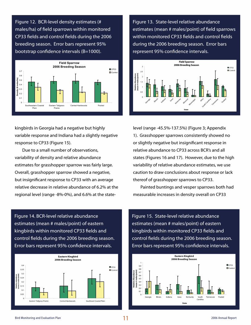
Figure 12. BCR-level density estimates (# males/ha) of field sparrows within monitored CP33 fields and
control fields during the 2006 breeding season ........................................................................................................................... 11
Figure 13. State-level relative abundance estimates (mean # males/point) of field sparrows within
monitored CP33 fields and control fields during the 2006 breeding season .................................................................... 11
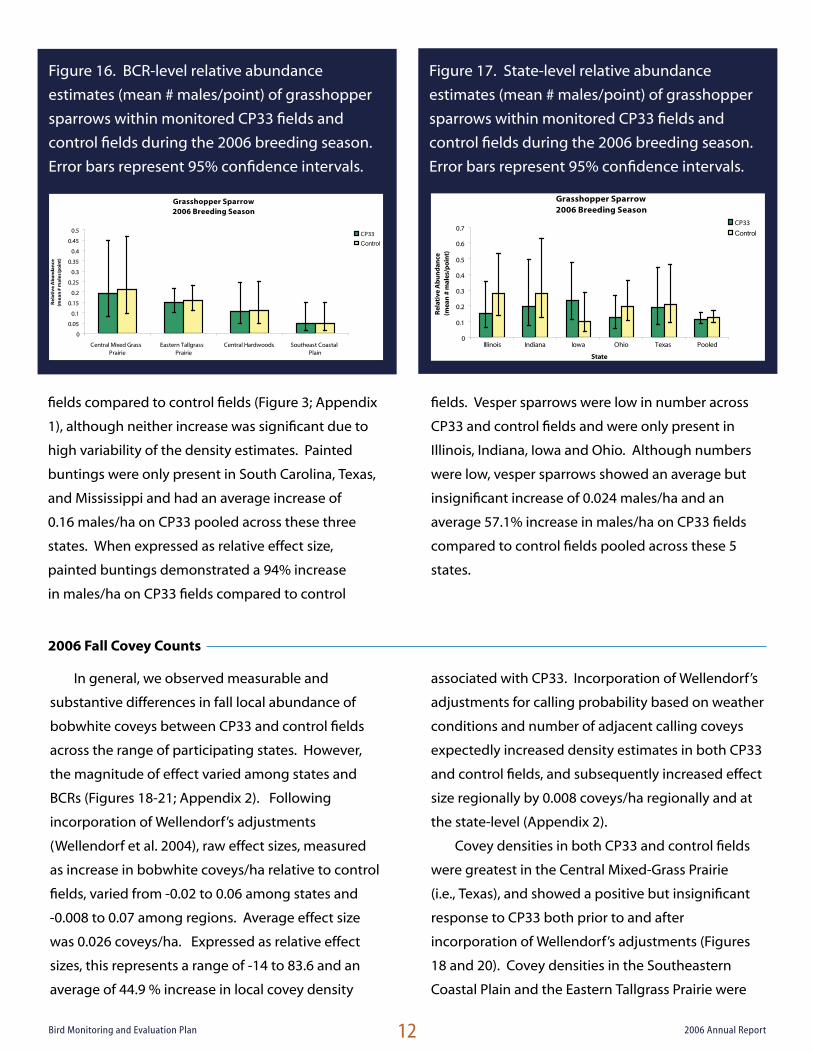
Figure 14. BCR-level relative abundance estimates (mean # males/point) of eastern kingbirds within
monitored CP33 fields and control fields during the 2006 breeding season .................................................................... 11
Figure 15. State-level relative abundance estimates (mean # males/point) of eastern kingbirds within
monitored CP33 fields and control fields during the 2006 breeding season .................................................................... 11
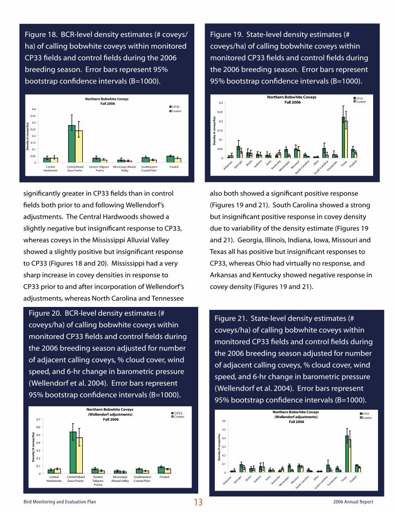
Figure 16. BCR-level relative abundance estimates (mean # males/point) of grasshopper sparrows within
monitored CP33 fields and control fields during the 2006 breeding season .................................................................... 12
Figure 17. State-level relative abundance estimates (mean # males/point) of grasshopper sparrows within
monitored CP33 fields and control fields during the 2006 breeding season .................................................................... 12
Table of ContentsFigure 18. BCR-level density estimates (# coveys/ha) of calling bobwhite coveys within monitored CP33
fields and control fields during the 2006 breeding season ...................................................................................................... 13
Figure 19. State-level density estimates (# coveys/ha) of calling bobwhite coveys within monitored CP33 fields and
control fields during the 2006 breeding season ........................................................................................................................... 13
Figure 20. BCR-level density estimates (# coveys/ha) of calling bobwhite coveys within monitored CP33 fields and
control fields during the 2006 breeding season adjusted for number of adjacent calling coveys, % cloud cover,
wind speed, and 6-hr change in barometric pressure (Wellendorf et al. 2004) ................................................................ 13
Figure 21. State-level density estimates (# coveys/ha) of calling bobwhite coveys within monitored CP33 fields
and control fields during the 2006 breeding season adjusted for number of adjacent calling coveys, % cloud cover,
wind speed, and 6-hr change in barometric pressure (Wellendorf et al. 2004) ................................................................ 13
List of Appendices
Appendix 1. BCR and state-level density (# males/ha) or relative abundance (mean # males/point) estimates,
standard error, raw effect size, 95% confidence intervals for effect size, and relative effect size for species of
interest within monitored CP33 fields and control fields during the 2006 breeding season...................................... 21
Appendix 2. BCR and state-level density estimates (# coveys/ha), 95% bootstrap confidence intervals
(B=1000), and raw and relative effect sizes for calling bobwhite coveys within monitored CP33 fields and
control fields during the 2006 fall of 2006 and BCR and state-level density estimates adjusted for number of
adjacent calling coveys, % cloud cover, wind speed, and 6-hr change in barometric pressure (Wellendorf et al.
2004). 95% confidence intervals on effect size were included for unadjusted density estimates ........................... 28

1Bird Monitoring and Evaluation Plan 2006 Annual Report
IntroductionThe North American Breeding Bird Survey
(BBS), currently the only large-scale and long-term
measurement tool used to estimate population
trends of bird species in North America, provided
the first indication that grassland obligate and
successional-shrub dependent species in the United
States were experiencing a severe decline. BBS
results suggest that 43% of grassland species and
34% of successional-scrub species have exhibited
significant population declines since 1980 (Sauer
et al. 2006). Among these, some of the most
severe annual declines are found in populations
of Henslow’s sparrow (Ammodramus henslowii)
(5.7%), northern bobwhite (3.8%), grasshopper
sparrow (3.4%), eastern meadowlark (3.1%), and
field sparrow (2.4%) (Sauer et al. 2006). Contributing
to the cause of these declines is no doubt the
historical conversion of many native grasslands to
agricultural production, which is exacerbated today
by factors such as clean-farming techniques that
reduce the amount of fallow area around field edges,
urbanization, reforestation, and fire-exclusion. The
inevitable habitat changes that coincide with these
factors have resulted in the dependence of many
early-successional species on suboptimal habitat for
various parts of their life cycle.
In response to population recovery goals set by
the Northern Bobwhite Conservation Initiative (NBCI;
Dimmick et al. 2002), the Southeast Quail Study
Group has emphasized the development of methods
to increase bobwhite populations in agricultural
landscapes. To realistically attain the population
recovery goals, it is essential that management
practices coexist with agricultural production, and
hence avoid requiring producers to remove whole
fields from crop production. The implementation
of subsidized mixed native warm-season grass, forb,
and legume buffers around cropped fields may be
one method to increase bobwhite and other early-
successional songbird habitats with minimal or
positive economic impact on landowners (Barbour
et al 2007). In 2004, following recommendation
by the SEQSG, the USDA-Farm Service Agency
(FSA) implemented the Habitat Buffers for Upland
Birds (CP33) practice as part of the Continuous
Conservation Reserve Program (CRP). The FSA
allocated 250,000 CP33 acres to 35 states to be
actively managed over a period of 10 years.
As the majority of CRP practices were initially
established to decrease soil erosion and increase
water quality, the FSA raised concern about the
paucity of information regarding effects of CRP
practices on wildlife populations. To address these
concerns, the FSA charged the SEQSG with the
development of a CP33 monitoring program to
estimate bobwhite and priority songbird population
response to implementation of CP33 at a state,
regional and national level over a 3 year sampling
period. Subsequently, the “CP33-Habitat
Buffers for Upland Birds Monitoring
Protocol” was created and the
monitoring program commenced
during the 2006 breeding
season (Burger et
al.2006).
2Bird Monitoring and Evaluation Plan 2006 Annual Report
Methods
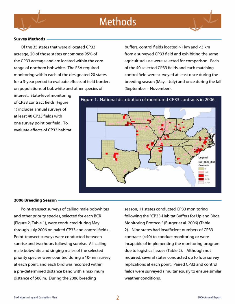
Of the 35 states that were allocated CP33
acreage, 20 of those states encompass 95% of
the CP33 acreage and are located within the core
range of northern bobwhite. The FSA required
monitoring within each of the designated 20 states
for a 3-year period to evaluate effects of field borders
on populations of bobwhite and other species of
interest. State-level monitoring
of CP33 contract fields (Figure
1) includes annual surveys of
at least 40 CP33 fields with
one survey point per field. To
evaluate effects of CP33 habitat
buffers, control fields located >1 km and <3 km
from a surveyed CP33 field and exhibiting the same
agricultural use were selected for comparison. Each
of the 40 selected CP33 fields and each matching
control field were surveyed at least once during the
breeding season (May – July) and once during the fall
(September – November).
Figure 1. National distribution of monitored CP33 contracts in 2006.
Point-transect surveys of calling male bobwhites
and other priority species, selected for each BCR
(Figure 2, Table 1), were conducted during May
through July 2006 on paired CP33 and control fields.
Point-transect surveys were conducted between
sunrise and two hours following sunrise. All calling
male bobwhite and singing males of the selected
priority species were counted during a 10-min survey
at each point, and each bird was recorded within
a pre-determined distance band with a maximum
distance of 500 m. During the 2006 breeding
season, 11 states conducted CP33 monitoring
following the “CP33-Habitat Buffers for Upland Birds
Monitoring Protocol” (Burger et al. 2006) (Table
2). Nine states had insufficient numbers of CP33
contracts (<40) to conduct monitoring or were
incapable of implementing the monitoring program
due to logistical issues (Table 2). Although not
required, several states conducted up to four survey
replications at each point. Paired CP33 and control
fields were surveyed simultaneously to ensure similar
weather conditions.
2006 Breeding Season
Survey Methods

3Bird Monitoring and Evaluation Plan 2006 Annual Report
Fall counts of calling bobwhite coveys were
conducted using point-transect sampling between
September and November 2006 (based on
geographic location) on paired CP33 and control
fields. Fourteen states conducted covey count
surveys during the fall of 2006, with 13 of those
states following the “CP33-Habitat Buffers for Upland
Birds Monitoring Protocol” (Burger et al. 2006).
Covey call surveys were conducted simultaneously
on paired CP33 and control fields from 45 min before
sunrise to 5 min before sunrise or until covey calls
had ceased. Covey locations and time of calling
were recorded on datasheets containing aerial
photos of the survey location. Distance was later
measured from georeferenced NAIP imagery in
ARCGIS to generate an exact radial distance from
the point to the estimated location of the calling
covey. In an effort to derive measures of density
that incorporated variable calling rates, number of
adjacent calling coveys and weather characteristics
(6-hr change in barometric pressure (1 am – 7 am; in/
Hg), percent cloud cover, and wind speed (km/hr))
were recorded during each survey (Wellendorf et al.
2004).
Figure 2. Geographic location of Bird Conservation Regions
included in the 2006 breeding and fall CP33 monitoring
program. BCR’s include Central Mixed Grass Prairie (19-CMP),
Oaks and Prairies (21-OP). Eastern Tallgrass Prairie (22-ETP),
Prairie-Hardwood Transition (23-PHT), Central Hardwoods
(24-CH), Western Gulf Coast Plain (25-WGCP), Mississippi
Alluvial Valley (26-MAV), Southeastern Coastal Plain (27-SCP),
and Piedmont (29-PIED).
Data Analysis
Analysis of 2006 breeding season
and fall covey count data was conducted
using a 3-tiered approach, with results
generated nationally (across bobwhite
range), regionally (within each BCR), and
within each state. Density estimates
were obtained for fall covey data, and
for species with adequate numbers
of detections in the breeding season
using program Distance 5.0 (Thomas
et al. 2006). Relative abundances were
estimated for species in the breeding
season with too few detections to
accurately estimate density.
2006 Fall Covey Counts
4Bird Monitoring and Evaluation Plan 2006 Annual Report
We used conventional distance sampling (CDS)
in program Distance 5.0 (Thomas et al. 2006) to
estimate a detection function for each species of
interest based on the probability of detecting a
singing male at a given radial distance (m) from
the survey point (Buckland et al. 2001). Species
of interest varied based on location (Table 1).
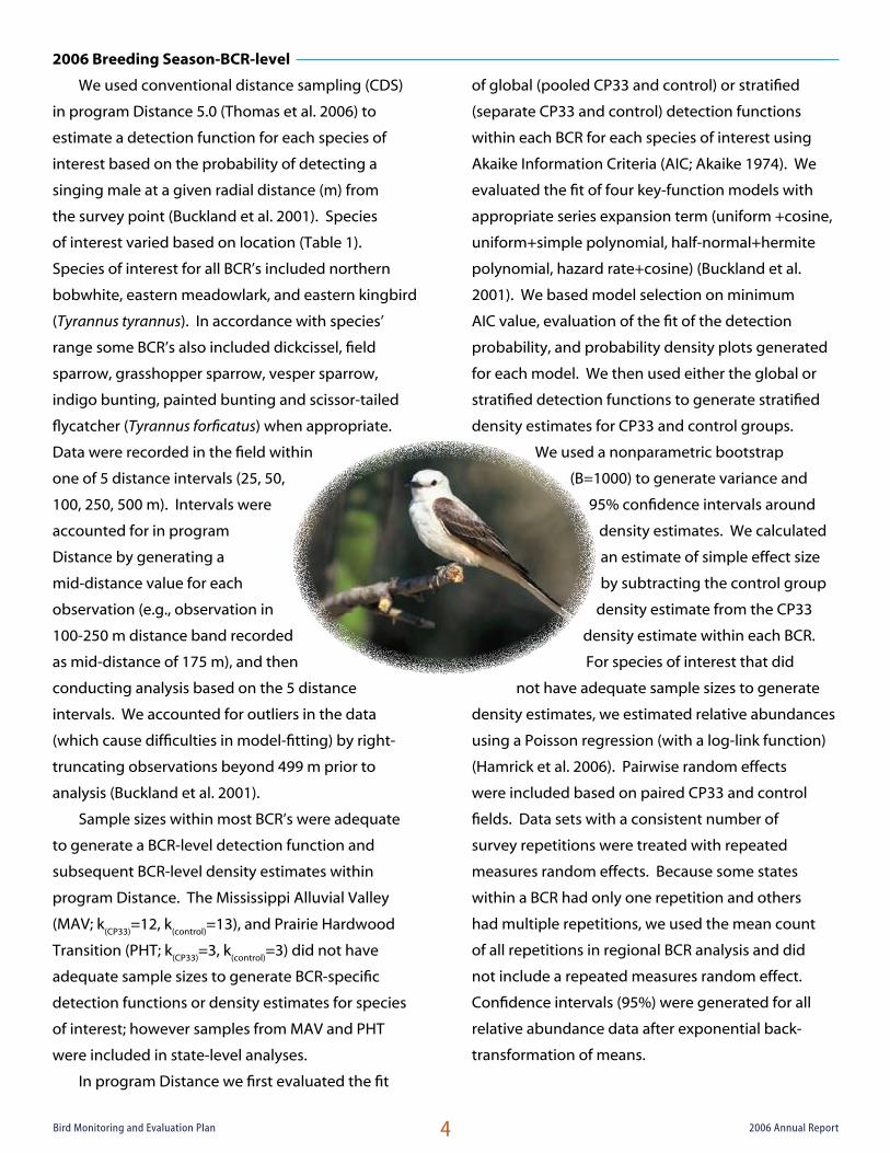
Species of interest for all BCR’s included northern
bobwhite, eastern meadowlark, and eastern kingbird
(Tyrannus tyrannus). In accordance with species’
range some BCR’s also included dickcissel, field
sparrow, grasshopper sparrow, vesper sparrow,
indigo bunting, painted bunting and scissor-tailed
flycatcher (Tyrannus forficatus) when appropriate.
Data were recorded in the field within
one of 5 distance intervals (25, 50,
100, 250, 500 m). Intervals were
accounted for in program
Distance by generating a
mid-distance value for each
observation (e.g., observation in
100-250 m distance band recorded
as mid-distance of 175 m), and then
conducting analysis based on the 5 distance
intervals. We accounted for outliers in the data
(which cause difficulties in model-fitting) by right-
truncating observations beyond 499 m prior to
analysis (Buckland et al. 2001).
Sample sizes within most BCR’s were adequate
to generate a BCR-level detection function and
subsequent BCR-level density estimates within
program Distance. The Mississippi Alluvial Valley
(MAV; k(CP33)
=12, k(control)
=13), and Prairie Hardwood
Transition (PHT; k(CP33)
=3, k(control)
=3) did not have
adequate sample sizes to generate BCR-specific
detection functions or density estimates for species
of interest; however samples from MAV and PHT
were included in state-level analyses.
In program Distance we first evaluated the fit
of global (pooled CP33 and control) or stratified
(separate CP33 and control) detection functions
within each BCR for each species of interest using
Akaike Information Criteria (AIC; Akaike 1974). We
evaluated the fit of four key-function models with
appropriate series expansion term (uniform +cosine,
uniform+simple polynomial, half-normal+hermite
polynomial, hazard rate+cosine) (Buckland et al.
2001). We based model selection on minimum
AIC value, evaluation of the fit of the detection
probability, and probability density plots generated
for each model. We then used either the global or
stratified detection functions to generate stratified
density estimates for CP33 and control groups.
We used a nonparametric bootstrap
(B=1000) to generate variance and
95% confidence intervals around
density estimates. We calculated
an estimate of simple effect size
by subtracting the control group
density estimate from the CP33
density estimate within each BCR.
For species of interest that did
not have adequate sample sizes to generate
density estimates, we estimated relative abundances
using a Poisson regression (with a log-link function)
(Hamrick et al. 2006). Pairwise random effects
were included based on paired CP33 and control
fields. Data sets with a consistent number of
survey repetitions were treated with repeated
measures random effects. Because some states
within a BCR had only one repetition and others
had multiple repetitions, we used the mean count
of all repetitions in regional BCR analysis and did
not include a repeated measures random effect.
Confidence intervals (95%) were generated for all
relative abundance data after exponential back-
transformation of means.
2006 Breeding Season-BCR-level
5Bird Monitoring and Evaluation Plan 2006 Annual Report
There were not adequate sample sizes to
generate state-specific detection functions for
each species of interest based solely on within-
state data. However, Multiple Covariate Distance
Sampling (MCDS) in program Distance allows for the
estimation of detection functions at multiple levels.
Using this approach, we were able to generate state-
level density estimates for bobwhite, indigo bunting,
dickcissel, and eastern meadowlark. We first
used AIC model selection procedures in standard
CDS analysis (uniform+cosine, uniform+simple
polynomial, half normal+hermite polynomial and
hazard rate+cosine key functions) and determined
if stratified (CP33 and control separately) or global
detection functions better fit the national data set
for each species. If the model selected a stratified
detection function, we subsequently ran separate
analyses on each of the CP33 and control national
data sets for the species. If the model selected a
global detection function, we used the entire data
set for the species. Within the stratified (CP33 and
control) or global national data sets we then used
MCDS analysis (half-normal+hermite polynomial,
hazard rate+cosine key functions) to fit a global
model for the detection function, and used this
fitted model to estimate separate average state-
level detection functions using states as factor-level
covariates. We used these averaged state-level
detection functions to generate within-state density
estimates for species of interest for CP33 and control
groups. We used nonparametric bootstrap (B=1000)
to generate variance and 95% confidence intervals
around density estimates. We calculated a raw
estimate of effect size by subtracting the control
group density estimate from the CP33 density
estimate within each state. For species of interest
that did not have adequate sample sizes to generate
state-level density estimates, we instead estimated
relative abundances using the Poisson regression
methods outlined above. State-level relative
abundance estimates and 95% confidence intervals
were generated for eastern kingbird, field sparrow,
and grasshopper sparrow in 2006.
For the 2006 fall covey BCR-level analysis, we
used CDS methods (outlined above) in program
Distance to estimate a detection function based
on the probability of detecting a covey at a given
radial distance (m) from the survey point (Buckland
et al. 2001). The Piedmont (PIED; k(CP33)
=7, k(control)
=7),
Western Gulf Coastal Plain (WGCP; k(CP33)
=5, k(control)
=4),
and Prairie Hardwood Transition (PHT; k(CP33)
=3,
k(control)
=3) BCR’s did not have adequate sample sizes
to generate BCR-specific detection functions or
density estimates within program Distance; however
samples from PIED,WGCP, and PHT were included
in state-level analysis. We accounted for outliers in
the data (which cause difficulties in model-fitting) by
right-truncating the 10% of observations with largest
detection distances prior to analysis (Buckland et al.
2001). Analysis was conducted on ungrouped data
(i.e., using exact distances) on all but one BCR. The
Central Mixed Grass Prairie (CMP; also Texas) data
exhibited a substantial amount of heaping, and was
therefore analyzed using 6 distance intervals with
truncation at 380 m.
Within each BCR, we used AIC to evaluate the fit
of four key-function models with series expansions
(uniform +cosine, uniform+simple polynomial, half-
normal+hermite polynomial, hazard rate+cosine)
to determine if global (pooled CP33 and control)
or stratified (separate CP33 and control) detection
functions best fit the data. Similar to the breeding
season analysis, we based model selection on both
2006 Breeding Season- State-level
2006 Fall Covey Counts – BCR-level
6Bird Monitoring and Evaluation Plan 2006 Annual Report
the minimum AIC value and on evaluation of the fit
of the detection probability and probability density
plots generated for each model. The stratified
detection function (separate detection functions
for CP33 and control fields) exhibited the best
model fit in all but two BCR’s (Central Hardwoods
and Central Mixed Grass Prairie exhibited global
detection functions). We then used either the global
or stratified detection functions to generate stratified
density estimates for CP33 and control groups.
We used a nonparametric bootstrap (B=1000) to
generate variance and 95% confidence intervals
around density estimates. We calculated an estimate
of simple effect size by subtracting the control group
density estimate from the CP33 density estimate
within each BCR.
Incorporating Wellendorf’s adjustments.- With
apriori knowledge that extraneous factors in the
environment will influence calling rate of bobwhite
coveys, we also incorporated the adjustments
suggested by Wellendorf et al. (2004). We used a
logistic regression equation that incorporates the
number of adjacent calling coveys, 6-hr change
in barometric pressure (1am-7am; in/Hg), % cloud
cover, and wind speed (km/hr) during each survey
to estimate a calling probability. We interpreted the
posterior probability from the logistic regression as
a point-specific calling probability. We then divided
the number of coveys detected at a point by the
point-specific calling probability to generate an
adjusted point-specific estimate of total coveys. We
then used the global or stratified BCR-level detection
functions and the distance-based density estimation
equation (Buckland et al. 2001), ran a nonparametric
bootstrap (B=1000) and generated an average
adjusted density estimate and 95% confidence
intervals based on the 1000 bootstrap repetitions.
Similar to the breeding season analysis, there
were not adequate sample sizes to generate state-
specific detection functions based solely on within-
state data. We used MCDS in program Distance
to estimate multiple level detection functions
to generate state-specific density estimates. We
first used AIC model selection procedures in CDS
(uniform+cosine, uniform+simple polynomial,
half normal+hermite polynomial and hazard
rate+cosine key functions) and determined that
stratified detection functions (CP33 and control
specific) better fit the national covey data set. We
subsequently ran separate analyses on each of
the CP33 and control national data sets. Within
each of the CP33 and control national data sets we
used MCDS to fit a global model for the detection
function, and used this fitted model to estimate
separate average state-level detection functions
using states as factor-level covariates. We used
these averaged state-level detection functions to
generate within-state density estimates for CP33 and
control groups. We used nonparametric bootstrap
(B=1000) to generate variance and 95% confidence
intervals around density estimates. We calculated a
raw estimate of effect size by subtracting the control
group density estimate from the CP33 density
estimate within each state.
Incorporating Wellendorf’s adjustments.-Finally,
we used the logistic regression equation of
Wellendorf et al. (2004) to incorporate the number
of adjacent calling coveys, 6-hr change in barometric
pressure (1am-7am; in/Hg), % cloud cover, and
wind speed (km/hr) during each survey to estimate
a calling probability. We interpreted the posterior
probability from the logistic regression as point-level
calling probability. We then divided the number of
coveys detected at a point by the point-level calling
2006 Fall Covey Counts – State-level
7Bird Monitoring and Evaluation Plan 2006 Annual Report
Results
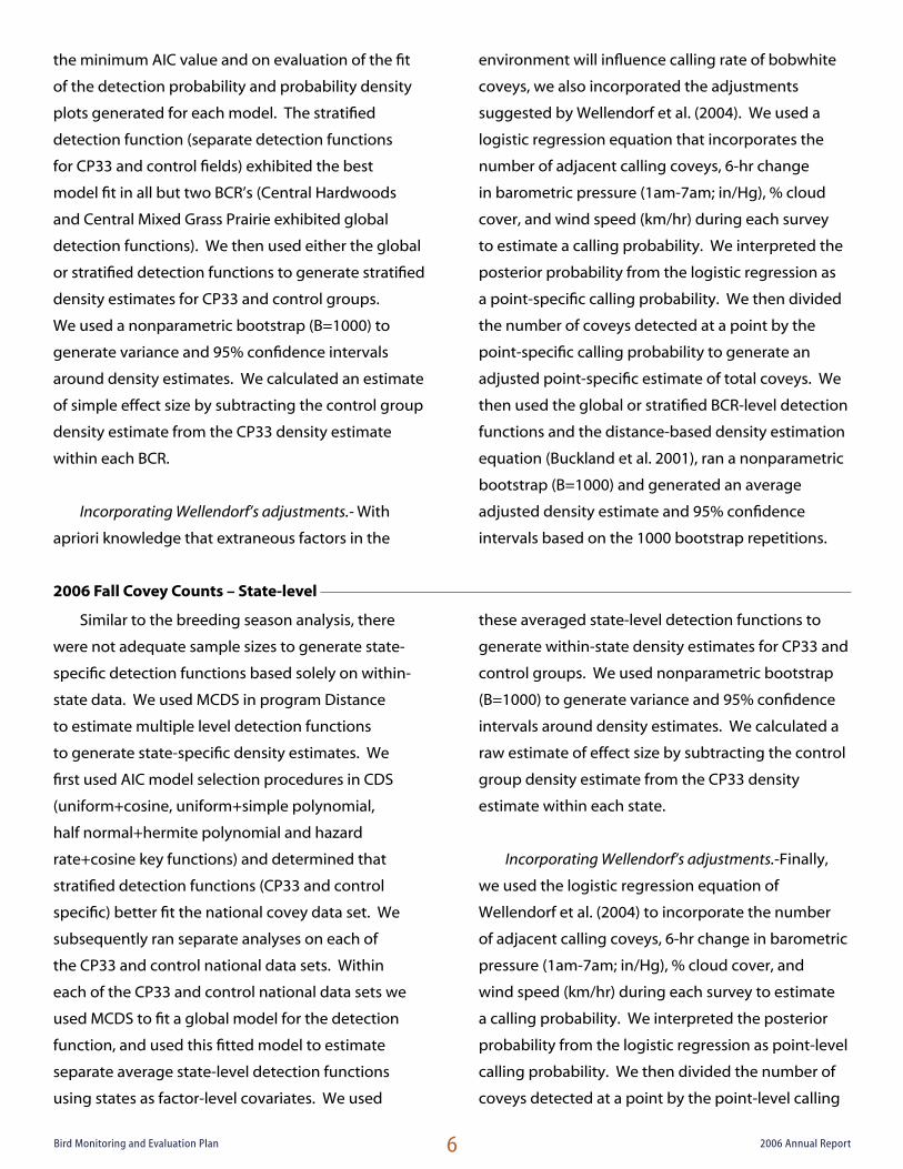
There were 98 total bird species detected in CP33
fields across all monitored states, 32 of which were
grassland obligate or early-successional specialist
species. There were 87 total species detected in
control fields, 26 of which were grassland obligates
or early-successional specialists. Response to CP33
varied among species and among BCR’s. Northern
bobwhite, indigo bunting, dickcissel, field sparrow,
painted bunting, and vesper sparrow had variable
positive responses to CP33, whereas eastern
kingbird, eastern meadowlark, and grasshopper
sparrow had relatively little or negative response
to CP33 (Figure 3). Significance of response was
determined by 95% confidence intervals on raw
effect sizes.
Northern bobwhite had a notable increase in
density with an average regional effect size of 0.05
males/ha (range -0.18-0.12) and an average state-
level effect size of 0.02 males/ha (range -0.13 – 0.07)
(Figure 3; Appendix 1). Regional relative effect size
was an average 36.7% increase in males/ha on CP33
(range -20.7%-171.6%), whereas state-level relative
effect size was an average 20.1% increase in males/
ha on CP33 (range -33.5% - 209.1%). An average
increase of 0.05 males/ha, converts to an average
increase of 1.2 male bobwhites per 10 acres on
CP33 fields compared to control fields. The Central
Mixed-Grass Prairie, which comprised Texas samples
only, had the greatest density of northern bobwhite,
but also showed negative response to CP33 in the
2006 breeding season (Figures 4 and 5). However,
low sample size in the CMP (<40 sample points per
treatment) resulted in a large degree of variation and
an effect size that did not differ from zero. Bobwhite
in the Southeastern Coastal Plain exhibited the
greatest positive response to CP33, whereas those
in the Central Hardwoods showed slightly positive
response, and in the Eastern Tallgrass Prairie had
little to no response (Figure 4). Bobwhite densities
were significantly greater on CP33 fields than control
in Georgia, Illinois, Kentucky, Mississippi and Missouri
(Figure 5). Point estimates of density were greater
but confidence intervals overlapped in Indiana, Iowa,
South Carolina, and Tennessee (Figure 5). In Ohio
Figure 3. Density estimates (# males/ha) of species
of interest within all monitored CP33 fields and
control fields during the 2006 breeding season.
Error bars represent 95% bootstrap confidence
intervals (B=1000).
Pooled2006 Breeding Season
0.00
0.50
1.00
1.50
2.00
2.50
DICK EAKI EAME FISP GRSP INBU NOBO PABU VESP
Species
Den
sity
(# m
ales
/ha)
CP33
Control
probability to generate an adjusted estimate of total coveys for each state. We then used the average state-level
detection functions generated by MCDS in program Distance and the distance-based density estimation equation
(Buckland et al. 2001) in a nonparametric bootstrap (B=1000) to generate average adjusted state-level density
estimates and 95% confidence intervals based on the 1000 bootstrap repetitions.
2006 Breeding Season

8Bird Monitoring and Evaluation Plan 2006 Annual Report
and Texas, point estimates of density were lower on
CP33 fields than control, but confidence intervals
overlapped (Figure 5). Note the difference in density
estimates for CMP (Figure 4) and Texas (Figure 5).
These densities are estimated from the same data
set (because CMP comprises only the Texas samples),
however, this is a good example of the difference
between estimating a detection function based
on the given data set alone (as in CMP; Figure 4),
compared to estimating the detection function in
MCDS as an averaged state-level detection function
based on a global detection function (as in TX; Figure
5). When sample size is adequate we recommend
estimating the detection function in CDS based off
the data set alone (as in CMP), and only using the
MCDS 2-level detection function method to estimate
densities for data-sets with sample sizes too low to
be estimated in CDS.
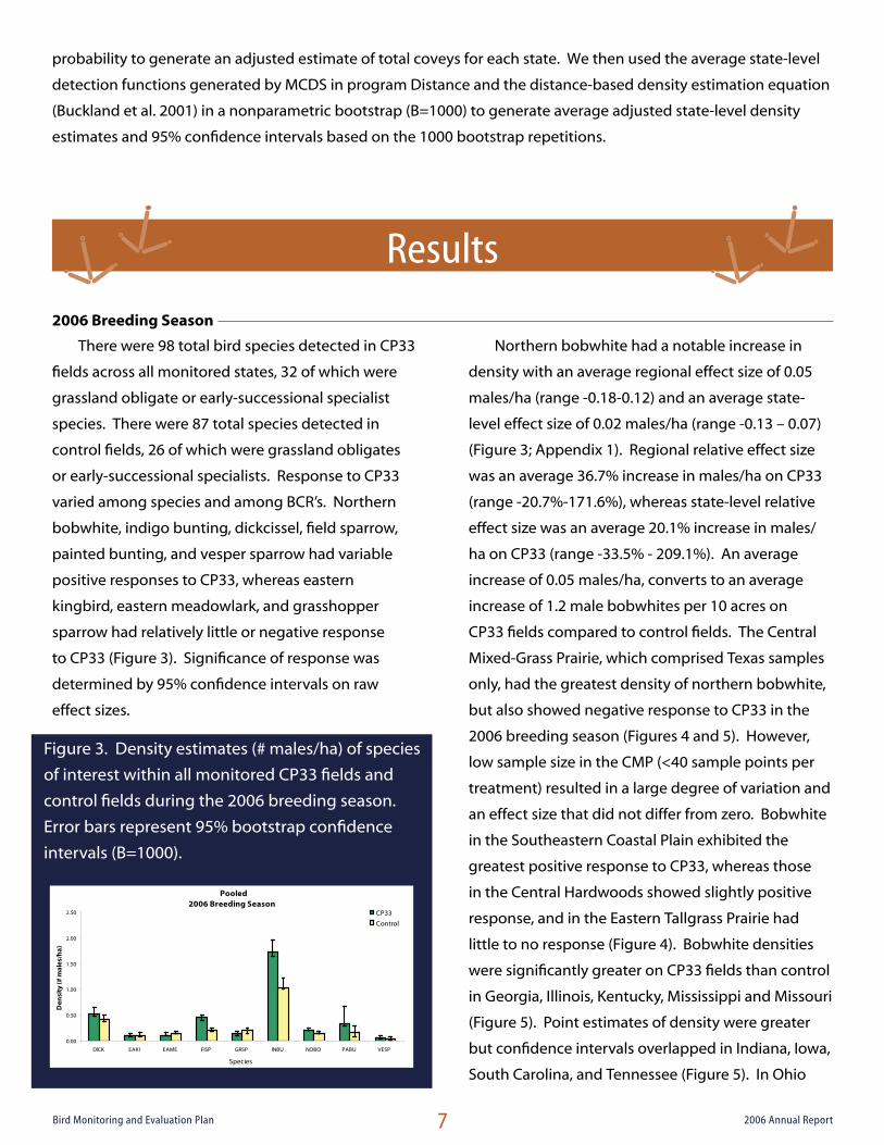
At both the regional level and state-level,
dickcissel exhibited an average relative effect size
of 28% on CP33, but confidence intervals included
zero (Figure 3; Appendix 1). Relative effect sizes
ranged from -20.7% to 171.6% at the regional level
and -33.5% to 209.1% at the state level. Average raw
effect size at the regional level was 0.12 males/ha
(range –0.04-0.35), and at the state level 0.06 males/
ha (-0.16-0.28) on CP33 fields when compared to
control fields. . Dickcissel displayed a substantive
positive response to CP33 in the Eastern Tallgrass
Prairie, and positive but not significant response
in the Southeastern Coastal Plain and Central
Hardwoods (Figure 6). Dickcissel showed a negative
response to CP33 in the Central Mixed-Grass Prairie
(Figure 6). Dickcissels in Illinois and Indiana exhibited
a strong positive response to CP33, whereas those
in Iowa, Kentucky, and Mississippi showed a positive
but insignificant response (Figure 7). Dickcissels in
Tennessee, Texas and Missouri had a negative but
insignificant response to CP33 (Figure 7).
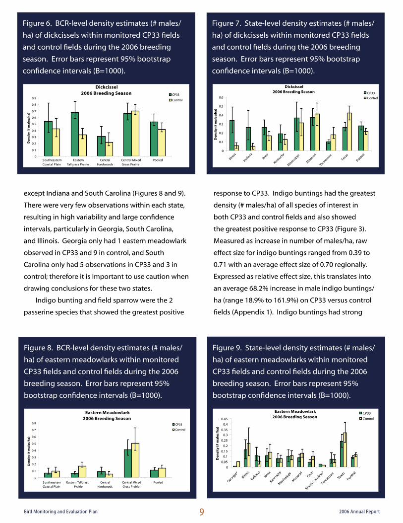
Eastern meadowlark exhibited a negative
response overall to CP33, with an average regional
decrease in density of 20.4% (range -63.7%-66%)
and an average state-level decrease in density of
19% (range -88.9%-88.3%) on CP33 fields when
compared to control fields (Figure 3; Appendix 1).
There was consistent lack of or negative response
of eastern meadowlark to CP33 across all BCR’s
except the Central Hardwoods, and across all states
Figure 4. BCR-level density estimates (# males/
ha) of northern bobwhite within monitored
CP33 fields and control fields during the 2006
breeding season. Error bars represent 95%
bootstrap confidence intervals (B=1000).
Northern Bobwhite 2006 Breeding Season
0
0.2
0.4
0.6
0.8
1
1.2
1.4
SoutheasternCoastal Plain
EasternTallgrass
Prairie
CentralHardwoods
Central MixedGrass Prairie
Pooled
Den
sity
(# m
ales
/ha)
CP33
Control
Figure 5. State-level density estimates (# males/
ha) of northern bobwhite within monitored
CP33 fields and control fields during the 2006
breeding season. Error bars represent 95%
bootstrap confidence intervals (B=1000).
Northern Bobwhite 2006 Breeding Season
0
0.1
0.2
0.3
0.4
0.5
0.6
0.7
Georgia
Illnois*
Indiana
Iowa
Kentucky
Miss
issip
pi
Miss
ouriOhio
South C
arolin
a
Tennessee
Texas
Pooled
Den
sity
(# m
ales
/ha)
CP33
Control
*The bootstrap confidence interval for Illinois control was not plausible; therefore the confidence interval presented for IL control was generated using program Distance.
9Bird Monitoring and Evaluation Plan 2006 Annual Report
except Indiana and South Carolina (Figures 8 and 9).
There were very few observations within each state,
resulting in high variability and large confidence
intervals, particularly in Georgia, South Carolina,
and Illinois. Georgia only had 1 eastern meadowlark
observed in CP33 and 9 in control, and South
Carolina only had 5 observations in CP33 and 3 in
control; therefore it is important to use caution when
drawing conclusions for these two states.
Indigo bunting and field sparrow were the 2
passerine species that showed the greatest positive
response to CP33. Indigo buntings had the greatest
density (# males/ha) of all species of interest in
both CP33 and control fields and also showed
the greatest positive response to CP33 (Figure 3).
Measured as increase in number of males/ha, raw
effect size for indigo buntings ranged from 0.39 to
0.71 with an average effect size of 0.70 regionally.
Expressed as relative effect size, this translates into
an average 68.2% increase in male indigo buntings/
ha (range 18.9% to 161.9%) on CP33 versus control
fields (Appendix 1). Indigo buntings had strong
Figure 8. BCR-level density estimates (# males/
ha) of eastern meadowlarks within monitored
CP33 fields and control fields during the 2006
breeding season. Error bars represent 95%
bootstrap confidence intervals (B=1000).
Eastern Meadowlark 2006 Breeding Season
0
0.1
0.2
0.3
0.4
0.5
0.6
0.7
0.8
SoutheasternCoastal Plain
Eastern TallgrassPrairie
CentralHardwoods
Central MixedGrass Prairie
Pooled
Den
sity
(# m
ales
/ha)
CP33
Control
Figure 9. State-level density estimates (# males/
ha) of eastern meadowlarks within monitored
CP33 fields and control fields during the 2006
breeding season. Error bars represent 95%
bootstrap confidence intervals (B=1000).
Eastern Meadowlark 2006 Breeding Season
0
0.05
0.1
0.15
0.2
0.25
0.3
0.35
0.4
0.45
Georgia*
Illnois
Indiana
Iowa
Kentucky
Miss
issip
pi
Miss
ouriOhio
South C
arolin
a*
Tennessee
Texas
Pooled
Den
sity
(# m
ales
/ha)
CP33
Control
Figure 6. BCR-level density estimates (# males/
ha) of dickcissels within monitored CP33 fields
and control fields during the 2006 breeding
season. Error bars represent 95% bootstrap
confidence intervals (B=1000).
Dickcissel 2006 Breeding Season
0
0.1
0.2
0.3
0.4
0.5
0.6
0.7
0.8
0.9
SoutheasternCoastal Plain
EasternTallgrass Prairie
CentralHardwoods
Central MixedGrass Prairie
Pooled
Den
sity
(# m
ales
/ha)
CP33
Control
Figure 7. State-level density estimates (# males/
ha) of dickcissels within monitored CP33 fields
and control fields during the 2006 breeding
season. Error bars represent 95% bootstrap
confidence intervals (B=1000).
Dickcissel 2006 Breeding Season
0
0.1
0.2
0.3
0.4
0.5
0.6
Illnois
Indiana
Iowa
Kentucky
Miss
issip
pi
Miss
ouri
Tennessee
Texas
Pooled
Den
sity
(# m
ales
/ha)
CP33
Control
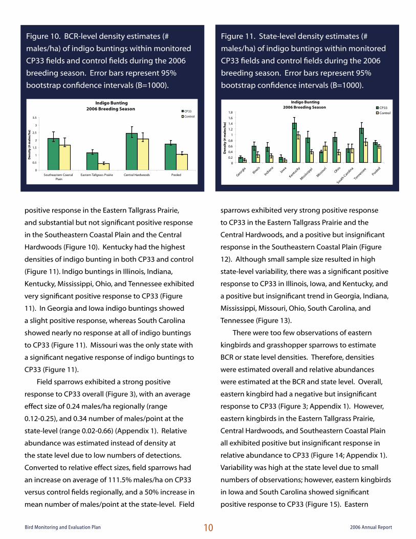
10Bird Monitoring and Evaluation Plan 2006 Annual Report
positive response in the Eastern Tallgrass Prairie,
and substantial but not significant positive response
in the Southeastern Coastal Plain and the Central
Hardwoods (Figure 10). Kentucky had the highest
densities of indigo bunting in both CP33 and control
(Figure 11). Indigo buntings in Illinois, Indiana,
Kentucky, Mississippi, Ohio, and Tennessee exhibited
very significant positive response to CP33 (Figure
11). In Georgia and Iowa indigo buntings showed
a slight positive response, whereas South Carolina
showed nearly no response at all of indigo buntings
to CP33 (Figure 11). Missouri was the only state with
a significant negative response of indigo buntings to
CP33 (Figure 11).
Field sparrows exhibited a strong positive
response to CP33 overall (Figure 3), with an average
effect size of 0.24 males/ha regionally (range
0.12-0.25), and 0.34 number of males/point at the
state-level (range 0.02-0.66) (Appendix 1). Relative
abundance was estimated instead of density at
the state level due to low numbers of detections.
Converted to relative effect sizes, field sparrows had
an increase on average of 111.5% males/ha on CP33
versus control fields regionally, and a 50% increase in
mean number of males/point at the state-level. Field
sparrows exhibited very strong positive response
to CP33 in the Eastern Tallgrass Prairie and the
Central Hardwoods, and a positive but insignificant
response in the Southeastern Coastal Plain (Figure
12). Although small sample size resulted in high
state-level variability, there was a significant positive
response to CP33 in Illinois, Iowa, and Kentucky, and
a positive but insignificant trend in Georgia, Indiana,
Mississippi, Missouri, Ohio, South Carolina, and
Tennessee (Figure 13).
There were too few observations of eastern
kingbirds and grasshopper sparrows to estimate
BCR or state level densities. Therefore, densities
were estimated overall and relative abundances
were estimated at the BCR and state level. Overall,
eastern kingbird had a negative but insignificant
response to CP33 (Figure 3; Appendix 1). However,
eastern kingbirds in the Eastern Tallgrass Prairie,
Central Hardwoods, and Southeastern Coastal Plain
all exhibited positive but insignificant response in
relative abundance to CP33 (Figure 14; Appendix 1).
Variability was high at the state level due to small
numbers of observations; however, eastern kingbirds
in Iowa and South Carolina showed significant
positive response to CP33 (Figure 15). Eastern
Figure 10. BCR-level density estimates (#
males/ha) of indigo buntings within monitored
CP33 fields and control fields during the 2006
breeding season. Error bars represent 95%
bootstrap confidence intervals (B=1000).
Indigo Bunting2006 Breeding Season
0
0.5
1
1.5
2
2.5
3
3.5
Southeastern CoastalPlain
Eastern Tallgrass Prairie Central Hardwoods Pooled
Den
sity
(# m
ales
/ha)
CP33
Control
Figure 11. State-level density estimates (#
males/ha) of indigo buntings within monitored
CP33 fields and control fields during the 2006
breeding season. Error bars represent 95%
bootstrap confidence intervals (B=1000).
Indigo Bunting 2006 Breeding Season
0
0.2
0.4
0.6
0.8
1
1.2
1.4
1.6
1.8
Georgia
Illnois
Indiana
Iowa
Kentucky
Miss
issip
pi
Miss
ouriOhio
South C
arolin
a
Tennessee
Pooled
Den
sity
(# m
ales
/ha)
CP33
Control
11Bird Monitoring and Evaluation Plan 2006 Annual Report
kingbirds in Georgia had a negative but highly
variable response and Indiana had a slightly negative
response to CP33 (Figure 15).
Due to a small number of observations,
variability of density and relative abundance
estimates for grasshopper sparrow was fairly large.
Overall, grasshopper sparrow showed a negative,
but insignificant response to CP33 with an average
relative decrease in relative abundance of 6.2% at the
regional level (range -8%-0%), and 6.6% at the state-
level (range -45.5%-137.5%) (Figure 3; Appendix
1). Grasshopper sparrows consistently showed no
or slightly negative but insignificant response in
relative abundance to CP33 across BCR’s and all
states (Figures 16 and 17). However, due to the high
variability of relative abundance estimates, we use
caution to draw conclusions about response or lack
thereof of grasshopper sparrows to CP33.
Painted buntings and vesper sparrows both had
measurable increases in density overall on CP33
Figure 14. BCR-level relative abundance
estimates (mean # males/point) of eastern
kingbirds within monitored CP33 fields and
control fields during the 2006 breeding season.
Error bars represent 95% confidence intervals.
Eastern Kingbird2006 Breeding Season
0
0.05
0.1
0.15
0.2
0.25
0.3
0.35
0.4
Eastern Tallgrass Prairie Central Hardwoods Southeast Coastal Plain
Re
lati
ve
ab
un
da
nce
(me
an
# m
ale
s/p
oin
t)
CP33
Control
Figure 15. State-level relative abundance
estimates (mean # males/point) of eastern
kingbirds within monitored CP33 fields and
control fields during the 2006 breeding season.
Error bars represent 95% confidence intervals.
Eastern Kingbird2006 Breeding Season
0
0.1
0.2
0.3
0.4
0.5
0.6
0.7
0.8
0.9
1
Georgia Illinois Indiana Iowa Kentucky SouthCarolina
Tennessee Pooled
State
Rel
ativ
e A
bu
nd
ance
(mea
n #
mal
es/p
oin
t)
CP33
Control
Figure 12. BCR-level density estimates (#
males/ha) of field sparrows within monitored
CP33 fields and control fields during the 2006
breeding season. Error bars represent 95%
bootstrap confidence intervals (B=1000).
Field Sparrow 2006 Breeding Season
0
0.1
0.2
0.3
0.4
0.5
0.6
0.7
Southeastern CoastalPlain
Eastern TallgrassPrairie
Central Hardwoods Pooled
Den
sity
(# m
ales
/ha)
CP33
Control
Figure 13. State-level relative abundance
estimates (mean # males/point) of field sparrows
within monitored CP33 fields and control fields
during the 2006 breeding season. Error bars
represent 95% confidence intervals.
Field Sparrow2006 Breeding Season
0
0.5
1
1.5
2
2.5
3
Georgia
Illinois
Indiana
Iowa
Kentucky
Miss
ouri
Miss
issip
piOhio
South C
arolin
a
Tennessee
Pooled
State
Rel
ativ
e A
bu
nd
ance
(m
ean
# m
ales
/po
int)
CP33
Control
12Bird Monitoring and Evaluation Plan 2006 Annual Report
fields compared to control fields (Figure 3; Appendix
1), although neither increase was significant due to
high variability of the density estimates. Painted
buntings were only present in South Carolina, Texas,
and Mississippi and had an average increase of
0.16 males/ha on CP33 pooled across these three
states. When expressed as relative effect size,
painted buntings demonstrated a 94% increase
in males/ha on CP33 fields compared to control
fields. Vesper sparrows were low in number across
CP33 and control fields and were only present in
Illinois, Indiana, Iowa and Ohio. Although numbers
were low, vesper sparrows showed an average but
insignificant increase of 0.024 males/ha and an
average 57.1% increase in males/ha on CP33 fields
compared to control fields pooled across these 5
states.
Figure 16. BCR-level relative abundance
estimates (mean # males/point) of grasshopper
sparrows within monitored CP33 fields and
control fields during the 2006 breeding season.
Error bars represent 95% confidence intervals.
Grasshopper Sparrow 2006 Breeding Season
0
0.05
0.1
0.15
0.2
0.25
0.3
0.35
0.4
0.45
0.5
Central Mixed GrassPrairie
Eastern TallgrassPrairie
Central Hardwoods Southeast CoastalPlain
Re
lati
ve
Ab
un
da
nce
(m
ea
n #
ma
les/
po
int)
CP33
Control
Figure 17. State-level relative abundance
estimates (mean # males/point) of grasshopper
sparrows within monitored CP33 fields and
control fields during the 2006 breeding season.
Error bars represent 95% confidence intervals.
Grasshopper Sparrow 2006 Breeding Season
0
0.1
0.2
0.3
0.4
0.5
0.6
0.7
Illinois Indiana Iowa Ohio Texas Pooled
State
Rel
ativ
e A
bu
nd
ance
(mea
n #
mal
es/p
oin
t)
CP33
Control
2006 Fall Covey Counts
In general, we observed measurable and
substantive differences in fall local abundance of
bobwhite coveys between CP33 and control fields
across the range of participating states. However,
the magnitude of effect varied among states and
BCRs (Figures 18-21; Appendix 2). Following
incorporation of Wellendorf’s adjustments
(Wellendorf et al. 2004), raw effect sizes, measured
as increase in bobwhite coveys/ha relative to control
fields, varied from -0.02 to 0.06 among states and
-0.008 to 0.07 among regions. Average effect size
was 0.026 coveys/ha. Expressed as relative effect
sizes, this represents a range of -14 to 83.6 and an
average of 44.9 % increase in local covey density
associated with CP33. Incorporation of Wellendorf’s
adjustments for calling probability based on weather
conditions and number of adjacent calling coveys
expectedly increased density estimates in both CP33
and control fields, and subsequently increased effect
size regionally by 0.008 coveys/ha regionally and at
the state-level (Appendix 2).
Covey densities in both CP33 and control fields
were greatest in the Central Mixed-Grass Prairie
(i.e., Texas), and showed a positive but insignificant
response to CP33 both prior to and after
incorporation of Wellendorf’s adjustments (Figures
18 and 20). Covey densities in the Southeastern
Coastal Plain and the Eastern Tallgrass Prairie were
13Bird Monitoring and Evaluation Plan 2006 Annual Report
significantly greater in CP33 fields than in control
fields both prior to and following Wellendorf’s
adjustments. The Central Hardwoods showed a
slightly negative but insignificant response to CP33,
whereas coveys in the Mississippi Alluvial Valley
showed a slightly positive but insignificant response
to CP33 (Figures 18 and 20). Mississippi had a very
sharp increase in covey densities in response to
CP33 prior to and after incorporation of Wellendorf’s
adjustments, whereas North Carolina and Tennessee
also both showed a significant positive response
(Figures 19 and 21). South Carolina showed a strong
but insignificant positive response in covey density
due to variability of the density estimate (Figures 19
and 21). Georgia, Illinois, Indiana, Iowa, Missouri and
Texas all has positive but insignificant responses to
CP33, whereas Ohio had virtually no response, and
Arkansas and Kentucky showed negative response in
covey density (Figures 19 and 21).
Figure 18. BCR-level density estimates (# coveys/
ha) of calling bobwhite coveys within monitored
CP33 fields and control fields during the 2006
breeding season. Error bars represent 95%
bootstrap confidence intervals (B=1000).
Northern Bobwhite CoveysFall 2006
0
0.05
0.1
0.15
0.2
0.25
0.3
0.35
0.4
CentralHardwoods
Central MixedGrass Prairie
Eastern TallgrassPrairie
Mississippi AlluvialValley
SoutheasternCoastal Plain
Pooled
Den
sity
(# c
ove
ys/h
a)
CP33Control
Figure 19. State-level density estimates (#
coveys/ha) of calling bobwhite coveys within
monitored CP33 fields and control fields during
the 2006 breeding season. Error bars represent
95% bootstrap confidence intervals (B=1000).
Northern Bobwhite CoveysFall 2006
0
0.05
0.1
0.15
0.2
0.25
0.3
Arkansa
s
Georgia
Illnois
Indiana
Iowa
Kentucky
Miss
issip
pi
Miss
ouri
North C
arolin
aOhio
South C
arolin
a
Tennessee
Texas
Pooled
Den
sity
(# c
ove
ys/h
a)
CP33Control
Figure 20. BCR-level density estimates (#
coveys/ha) of calling bobwhite coveys within
monitored CP33 fields and control fields during
the 2006 breeding season adjusted for number
of adjacent calling coveys, % cloud cover, wind
speed, and 6-hr change in barometric pressure
(Wellendorf et al. 2004). Error bars represent
95% bootstrap confidence intervals (B=1000).
Northern Bobwhite Coveys(Wellendorf adjustments)
Fall 2006
0
0.1
0.2
0.3
0.4
0.5
0.6
0.7
CentralHardwoods
Central MixedGrass Prairie
EasternTallgrass
Prairie
MississippiAlluvial Valley
SoutheasternCoastal Plain
Pooled
Den
sity
(# c
ove
ys/h
a)
CP33Control
Figure 21. State-level density estimates (#
coveys/ha) of calling bobwhite coveys within
monitored CP33 fields and control fields during
the 2006 breeding season adjusted for number
of adjacent calling coveys, % cloud cover, wind
speed, and 6-hr change in barometric pressure
(Wellendorf et al. 2004). Error bars represent
95% bootstrap confidence intervals (B=1000).Northern Bobwhite Coveys
(Wellendorf adjustments)Fall 2006
0
0.1
0.2
0.3
0.4
0.5
0.6
Arkansa
s
Georgia
Illnois
Indiana
Iowa
Kentucky
Miss
issip
pi
Miss
ouri
North C
arolin
aOhio
South C
arolin
a
Tennessee
Texas
Pooled
Den
sity
(# c
ove
ys/h
a)
CP33
Control
14Bird Monitoring and Evaluation Plan 2006 Annual Report
Upland habitat buffers are just one of many
available USDA conservation practices; however,
the CP33 practice is unique in that its central
focus is increasing abundance and diversity of
grassland avifauna in the agricultural landscape.
Prior to implementation of the CP33 monitoring
program, there had never been a large scale effort
to measure response of priority bird species’ to a
USDA conservation practice. Though they provided
important contributions to the understanding of
population response to agricultural conservation
practices, the majority of studies that examined
the effects of conservation buffers on wildlife
populations have been conducted at the farm or
local landscape scale, and have limited inferential
space (e.g., Marcus et al. 2000, Puckett et al. 2000,
Smith 2004, Conover 2005, Smith et al. 2005a,
2005b). Johnson and Igl (2001) used a regional
approach as they examined response of grassland
birds to the Conservation Reserve program, but
were still limited in that they only examined CRP
fields in 9 counties in eastern Montana, North and
South Dakota, and Western Minnesota. With the
implementation of CP33 Habitat Buffers for Upland
birds, and the CP33 monitoring program, we are
now able to contribute a large-scale multi-state
monitoring effort to the literature base.
We observed a positive overall response to
establishment of CP33 habitat buffers on northern
bobwhite populations, as well as populations
of several priority songbird species. Population
response varied, quite expectedly, by BCR and
state. This variation in response is likely due to a
multitude of factors, which include variation of the
establishment and growth of the buffers in their
first growing season due to weather conditions,
lack of dispersal to and colonization of buffers by
local avifauna, or differences in regional habitat
preferences by the bird community. There have
been several anecdotal accounts involving lack of
cover establishment or growth of buffers in the 2006
breeding season, often due to drought conditions.
Often the establishment of cover in the first year,
and on occasion in the second year, was critically
dependent on the amount of rainfall received in that
region.
The greatest densities of male bobwhite and
calling bobwhite coveys during 2006 on both
CP33 and control sites occurred in the CMP (i.e.,
Texas). However, the greatest significant positive
response to CP33 habitat buffers occurred in the
SCP in the 2006 breeding season and in the SCP
and ETP the following fall. It is important to note
that there was virtually no effect on density of
calling males in the ETP during the 2006 breeding
season, but there was a significant positive effect
on density of calling coveys during the following
fall. Additionally, although the response in both
Interpretation
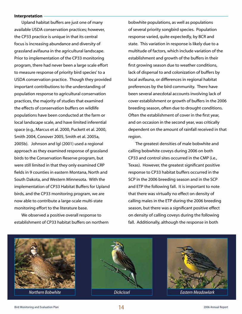
Northern Bobwhite Dickcissel Eastern Meadowlark

15Bird Monitoring and Evaluation Plan 2006 Annual Report
the breeding season and fall was variable, there
was a shift in the CMP from greater densities in
the control fields in the 2006 breeding season, to
greater densities in the CP33 fields the following
fall. This may support previous suggestions that
fall populations of bobwhite are more responsive
to field border practices than breeding populations
(Puckett et al. 2000, Smith 2004, Palmer et al. 2005).
If these differences in local abundance represent
actual increases in recruitment/population levels
attributable to CP33, instead of merely redistribution
of extant populations, CP33 has achieved remarkable
success in just its first 2 years of implementation.
A population response of this magnitude is
substantive, given that at the field and farm scale
CP33 typically represents only a 2 – 10% change in
land use.
Translating field-level effect sizes into
programmatic contributions to national bobwhite
populations is more problematic and requires some
assumptions regarding factors as yet unknown. The
following discussion is based on robust estimates of
field-level densities, but speculative with regard to
the total contribution of CP33 to national bobwhite
populations. As such, it should be taken as an
illustration of potential effect, not an estimate of
actual effect. Our estimates of effect size (0.026
coveys/ha) reflect differences in bobwhite covey
density at the spatial scale of the enrolled field.
Assuming an effective survey radius of 500 m or 78.5
ha (194 ac) this 0.026 coveys/ha difference translates
to an average 2.04 coveys more in the 194 ac region
surveyed around CP33 enrolled fields. Given a mean
October covey size of 12 birds, this would mean
24.48 more birds around CP33 fields than control
fields. The FSA national database report that as
of September 2007, 168,743 acres were enrolled
in CP33. However, although the total number of
contracts is known, the number of fields enrolled in
CP33 and the average number of buffer acres/field
is unknown. From our stratified sample of contracts
we will be able to use a cluster sampling approach
to estimate the total and mean number of fields/
contract and the mean acreage/buffered field. We
have not yet pursued that analysis. However, for
illustrative purposes, a hypothetical 40 ac square
field buffered with a 60’ buffer would have 6.9 acres
of buffer. The national enrollment of 168,743 acres
could accommodate 24,456 such hypothetical 40 ac
fields with 60’ buffers. Assuming 24.48 additional
birds in the fall population/CP33 field and no overlap
of 194 ac regions around CP33 fields (unrealistic
given aggregated distribution of CP33) this would
translate to 598,671 additional birds, or 3.5 birds/ac
CP33 enrolled.
It must be noted that ideally during the fall covey
surveys, coveys would be located and number of
individuals within each covey counted. However,
this is a very difficult and labor intensive task, and
also subjects the birds to unnecessary disturbance
and stress. Although counting the number of calling
coveys alone can provide useful estimates of covey
abundance, without flushing coveys it is impossible
to ascertain the number of individuals in a covey
Indigo Bunting Field Sparrow Eastern Kingbird Grasshopper Sparrow

16Bird Monitoring and Evaluation Plan 2006 Annual Report
(e.g., is it two coveys with 3 birds each or one covey
of 6 birds). This may limit our ability to extrapolate
information relative to population size.
Although bobwhite populations are
experiencing one of the most severe declines of all
grassland bird species, in reality it is an entire suite
of species that are dependent on grasslands or
early successional habitat for all or part of their life
cycle. Some early-successional species responded
dramatically to CP33, whereas others showed
virtually no or consistently negative response.
Dickcissel, field sparrow, indigo bunting and painted
bunting all showed positive response to CP33
with regional relative effect sizes reaching up to a
162% increase in density relative to control fields.
Additionally, although the number of vesper sparrow
detections was low across CP33 and control fields
in their range, they showed a significant and very
promising positive response to establishment of
CP33 buffers. Relative effect size for vesper sparrow
resulted in an average 51% increase in the number
of males/ha on CP33 in 2006. These five species,
which cover a range of habitat preferences from
grassland obligate to grass-shrub species, all exhibit
a distinct preference for crop fields bordered by CP33
compared to edge-to-edge cropping methods. This
positive response may be the result of increased and
variable nesting or foraging cover provided by, or the
changing insect community or seed base associated
with CP33 buffers.
Eastern meadowlark and grasshopper
sparrow were the only two species of interest
that consistently exhibited greater densities in
control rather than CP33 sites. These results are
discouraging in that both eastern meadowlark and
grasshopper sparrow populations are experiencing
sharp range-wide declines (3.1% and 3.4% annually
respectively; Sauer et al. 2006). However, this result
is not unexpected, because both species have a
tendency to be area-sensitive (Herkert 1994, Vickery
et al. 1994, Johnson and Igl 2001, Bakker et al.
2002), and thus show preferences for large tracts of
continuous grassland. However, there have also
been some instances where area sensitivity was not
an issue for these species, and densities were either
highly dependent on vegetation characteristics
(grasshopper sparrow) or did not depend on either
amount of area or vegetation characteristics (eastern
meadowlark) (Winter and Faaborg 1999). Herkert
(1994) estimated the area requirement for an
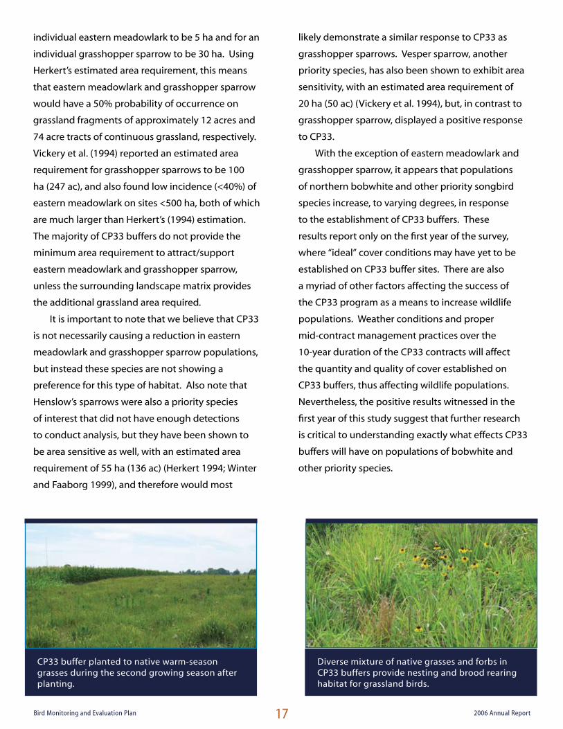
CP33 buffer planted to native warm-season grasses during the first growing season after planting.
17Bird Monitoring and Evaluation Plan 2006 Annual Report
individual eastern meadowlark to be 5 ha and for an
individual grasshopper sparrow to be 30 ha. Using
Herkert’s estimated area requirement, this means
that eastern meadowlark and grasshopper sparrow
would have a 50% probability of occurrence on
grassland fragments of approximately 12 acres and
74 acre tracts of continuous grassland, respectively.
Vickery et al. (1994) reported an estimated area
requirement for grasshopper sparrows to be 100
ha (247 ac), and also found low incidence (<40%) of
eastern meadowlark on sites <500 ha, both of which
are much larger than Herkert’s (1994) estimation.
The majority of CP33 buffers do not provide the
minimum area requirement to attract/support
eastern meadowlark and grasshopper sparrow,
unless the surrounding landscape matrix provides
the additional grassland area required.
It is important to note that we believe that CP33
is not necessarily causing a reduction in eastern
meadowlark and grasshopper sparrow populations,
but instead these species are not showing a
preference for this type of habitat. Also note that
Henslow’s sparrows were also a priority species
of interest that did not have enough detections
to conduct analysis, but they have been shown to
be area sensitive as well, with an estimated area
requirement of 55 ha (136 ac) (Herkert 1994; Winter
and Faaborg 1999), and therefore would most
likely demonstrate a similar response to CP33 as
grasshopper sparrows. Vesper sparrow, another
priority species, has also been shown to exhibit area
sensitivity, with an estimated area requirement of
20 ha (50 ac) (Vickery et al. 1994), but, in contrast to
grasshopper sparrow, displayed a positive response
to CP33.
With the exception of eastern meadowlark and
grasshopper sparrow, it appears that populations
of northern bobwhite and other priority songbird
species increase, to varying degrees, in response
to the establishment of CP33 buffers. These
results report only on the first year of the survey,
where “ideal” cover conditions may have yet to be
established on CP33 buffer sites. There are also
a myriad of other factors affecting the success of
the CP33 program as a means to increase wildlife
populations. Weather conditions and proper
mid-contract management practices over the
10-year duration of the CP33 contracts will affect
the quantity and quality of cover established on
CP33 buffers, thus affecting wildlife populations.
Nevertheless, the positive results witnessed in the
first year of this study suggest that further research
is critical to understanding exactly what effects CP33
buffers will have on populations of bobwhite and
other priority species.
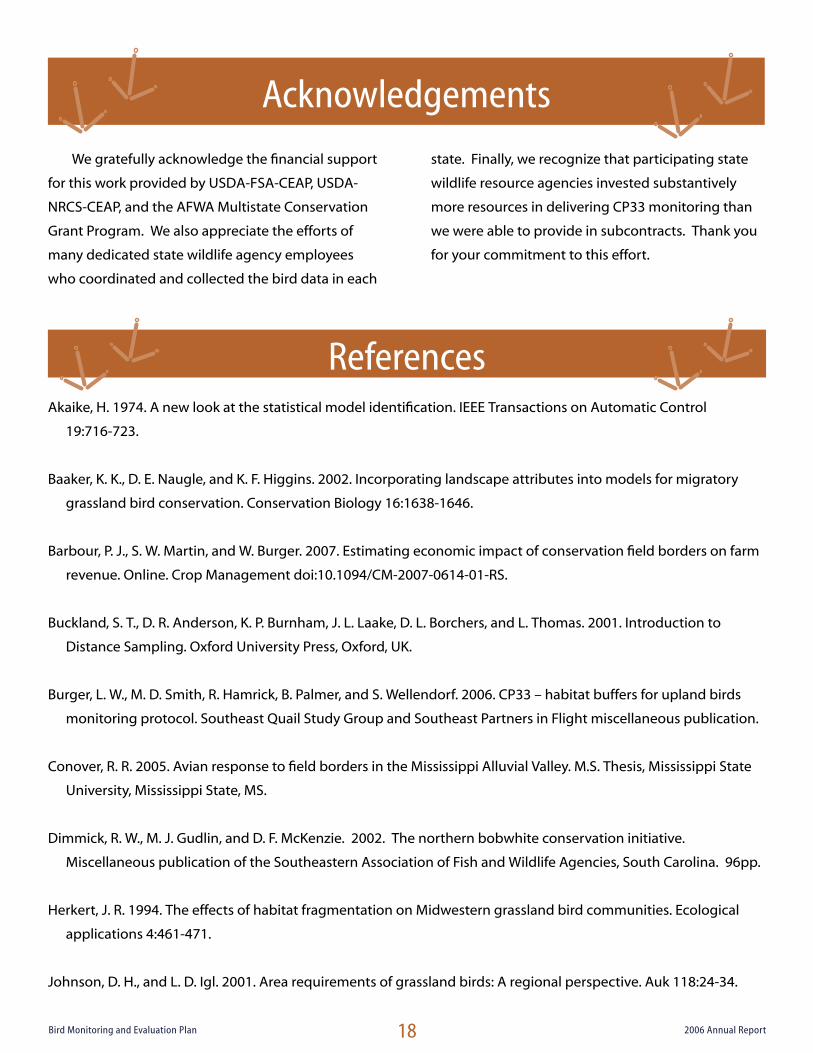
Diverse mixture of native grasses and forbs in CP33 buffers provide nesting and brood rearing habitat for grassland birds.
CP33 buffer planted to native warm-season grasses during the second growing season after planting.
18Bird Monitoring and Evaluation Plan 2006 Annual Report
Acknowledgements
We gratefully acknowledge the financial support
for this work provided by USDA-FSA-CEAP, USDA-
NRCS-CEAP, and the AFWA Multistate Conservation
Grant Program. We also appreciate the efforts of
many dedicated state wildlife agency employees
who coordinated and collected the bird data in each
state. Finally, we recognize that participating state
wildlife resource agencies invested substantively
more resources in delivering CP33 monitoring than
we were able to provide in subcontracts. Thank you
for your commitment to this effort.
ReferencesAkaike, H. 1974. A new look at the statistical model identification. IEEE Transactions on Automatic Control
19:716-723.
Baaker, K. K., D. E. Naugle, and K. F. Higgins. 2002. Incorporating landscape attributes into models for migratory
grassland bird conservation. Conservation Biology 16:1638-1646.
Barbour, P. J., S. W. Martin, and W. Burger. 2007. Estimating economic impact of conservation field borders on farm
revenue. Online. Crop Management doi:10.1094/CM-2007-0614-01-RS.
Buckland, S. T., D. R. Anderson, K. P. Burnham, J. L. Laake, D. L. Borchers, and L. Thomas. 2001. Introduction to
Distance Sampling. Oxford University Press, Oxford, UK.
Burger, L. W., M. D. Smith, R. Hamrick, B. Palmer, and S. Wellendorf. 2006. CP33 – habitat buffers for upland birds
monitoring protocol. Southeast Quail Study Group and Southeast Partners in Flight miscellaneous publication.
Conover, R. R. 2005. Avian response to field borders in the Mississippi Alluvial Valley. M.S. Thesis, Mississippi State
University, Mississippi State, MS.
Dimmick, R. W., M. J. Gudlin, and D. F. McKenzie. 2002. The northern bobwhite conservation initiative.
Miscellaneous publication of the Southeastern Association of Fish and Wildlife Agencies, South Carolina. 96pp.
Herkert, J. R. 1994. The effects of habitat fragmentation on Midwestern grassland bird communities. Ecological
applications 4:461-471.
Johnson, D. H., and L. D. Igl. 2001. Area requirements of grassland birds: A regional perspective. Auk 118:24-34.
19Bird Monitoring and Evaluation Plan 2006 Annual Report
Marcus, J. F., W. E. Palmer, and P. T. Bromley. 2000. The effects of farm field borders on overwintering sparrow
densities. Wilson Bulletin 112:517–523.
Palmer, W. E., S. D. Wellendorf, J. R. Gillis, and P. T. Bromley. 2005. Effect of field borders and nest predator reduction
on abundance of northern bobwhites. Wildlife Society Bulletin 33:1398-1405.
Puckett, K. M., W. E. Palmer, P. T. Bromley, J. R. Anderson, Jr., and T. L. Sharpe. 2000. Effect of filter strips on habitat
use and home range of northern bobwhites on Alligator National Wildlife Refuge. Proceedings of the National
Quail Symposium 4:26-31.
Sauer, J. R., J. E. Hines, and J. Fallon. 2006. The North American Breeding Bird Survey, Results and Analysis 1966 -
2006. Version 6.2.2006. USGS Patuxent Wildlife Research Center, Laurel, MD
Smith, M. D. 2004. Wildlife habitats benefits of field border management practices in Mississippi. Ph. D.
Dissertation, Mississippi State University, Mississippi State, MS.
Smith, M. D., P. J. Barbour, L. W. Burger, Jr., and S. J. Dinsmore. 2005a. Density and diversity of overwintering birs in managed
field borders in Mississippi. Wilson Bulletin 117:258-269.
Smith, M. D., P. J. Barbour, L. W. Burger, Jr., and S. J. Dinsmore. 2005b. Breeding bird abundance and diversity in agricultural
field borders in the black belt prairie of Mississippi. Proceeding of the Annual Conference of the Southeastern Association
of Fish and Wildlife Agencies 59:43-56.
Thomas, L., J. L. Laake, S. Strindberg, F. F. C. Marques, S. T. Buckand, D. L. Borchers, D. R. Anderson, K. P. Burnham, S. L. Hedley, J.
H. Pollard, J. R. B. Bishop, and T. A. Marques. 2006. Distance 5.0. Release 2. Research Unit for Wildlife Population Assessment,
University of St. Andrews, UK. http://www.ruwpa.st-and.ac.uk/distance/
Vickery, P. D., and M. L. Hunter, Jr. 1994. Effects of habitat area on the distribution of grassland birds in Maine. Conservation
Biology 8:1087-1097.
Wellendorf, S. D., W. E. Palmer, and P. T. Bromley. 2004. Estimating calling rates of northern bobwhite coveys and measuring
abundance. Journal of Wildlife Management 68:672-682.
Winter, M., and J. Faaborg. 1999. Patterns of area sensitivity in grassland-nesting birds. Conservation Biology 13:1424-1436.
During winter, native grasses in CP33 buffers provide roosting, foraging, and escape habitat for grassland birds.

20Bird Monitoring and Evaluation Plan 2006 Annual Report
Bird Conservation Region Species
19 - Central Mixed-grass Prairie
Bell’s Vireo, Dickcissel, Eastern Kingbird, Eastern Meadowlark, Field Sparrow, Grasshopper
Sparrow, Indigo Bunting, Northern Bobwhite, Painted Bunting, Scissor-tailed Flycatcher,
Upland Sandpiper
21 - Oaks and PrairiesBell’s Vireo, Dickcissel, Eastern Kingbird, Eastern Meadowlark, Field Sparrow, Indigo
Bunting, Northern Bobwhite, Painted Bunting, Scissor-tailed Flycatcher
22 - Eastern Tallgrass PrairieDickcissel, Eastern Kingbird, Eastern Meadowlark, Field Sparrow, Grasshopper Sparrow,
Indigo Bunting, Northern Bobwhite, Vesper Sparrow, Upland Sandpiper
23 - Prairie Hardwood TransitionDickcissel, Eastern Kingbird, Eastern Meadowlark, Field Sparrow, Indigo Bunting, Northern
Bobwhite, Vesper Sparrow
24 - Central HardwoodsDickcissel, Eastern Kingbird, Eastern Meadowlark, Field Sparrow, Indigo Bunting, Northern
Bobwhite
25 - Western Gulf Coast PlainDickcissel, Eastern Kingbird, Eastern Meadowlark, Indigo Bunting, Northern Bobwhite,
Painted Bunting
26 - Mississippi Alluvial ValleyDickcissel, Eastern Kingbird, Eastern Meadowlark, Field Sparrow, Grasshopper Sparrow,
Indigo Bunting, Northern Bobwhite, Painted Bunting
27 - Southeast Coastal PlainDickcissel, Eastern Kingbird, Eastern Meadowlark, Field Sparrow, Grasshopper Sparrow,
Indigo Bunting, Northern Bobwhite, Painted Bunting
29 - Piedmont Eastern Kingbird, Eastern Meadowlark, Field Sparrow, Indigo Bunting, Northern Bobwhite
Table 1. Species of interest selected for each Bird Conservation Region (BCR) for CP33 contract
monitoring in 2006.
Table 2. Distribution of CP33 monitoring during 2006 and 2007 breeding season and fall covey
counts.
Breeding Season and Fall
Covey Counts
CP33 monitoring (SEQSG
protocol)
CP33 monitoring
(other protocol)No CP33 monitoring
2006 Breeding SeasonGA, IA, IL, IN, KY, MO, MS,
OH, SC, TN, TX--
AL, AR, FL, KS, LA, NC, NE,
OK, VA
2006 Fall Covey CountsAR, GA, IA, IL, IN, KY, MO,
MS, NC, OH, SC, TN, TXKS AL, FL, LA, NE, OK, VA
2007 Breeding SeasonAR, GA, IA, IL, IN, KY MO,
MS, NC, OH, SC, TN, TX-- AL, FL, LA, OK, VA
2007 Fall Covey CountsAR, GA, IA, IL, IN, KY, MO,
MS, NC, NE, OH, SC, TN, TXKS AL, FL, LA, OK, VA
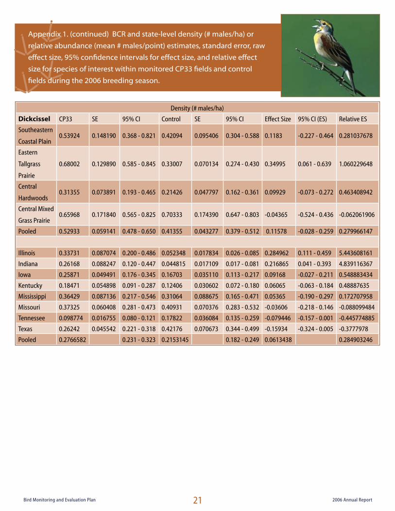
21Bird Monitoring and Evaluation Plan 2006 Annual Report
Density (# males/ha)
Dickcissel CP33 SE 95% CI Control SE 95% CI Effect Size 95% CI (ES) Relative ES
Southeastern
Coastal Plain0.53924 0.148190 0.368 - 0.821 0.42094 0.095406 0.304 - 0.588 0.1183 -0.227 - 0.464 0.281037678
Eastern
Tallgrass
Prairie
0.68002 0.129890 0.585 - 0.845 0.33007 0.070134 0.274 - 0.430 0.34995 0.061 - 0.639 1.060229648
Central
Hardwoods0.31355 0.073891 0.193 - 0.465 0.21426 0.047797 0.162 - 0.361 0.09929 -0.073 - 0.272 0.463408942
Central Mixed
Grass Prairie0.65968 0.171840 0.565 - 0.825 0.70333 0.174390 0.647 - 0.803 -0.04365 -0.524 - 0.436 -0.062061906
Pooled 0.52933 0.059141 0.478 - 0.650 0.41355 0.043277 0.379 - 0.512 0.11578 -0.028 - 0.259 0.279966147
Illinois 0.33731 0.087074 0.200 - 0.486 0.052348 0.017834 0.026 - 0.085 0.284962 0.111 - 0.459 5.443608161
Indiana 0.26168 0.088247 0.120 - 0.447 0.044815 0.017109 0.017 - 0.081 0.216865 0.041 - 0.393 4.839116367
Iowa 0.25871 0.049491 0.176 - 0.345 0.16703 0.035110 0.113 - 0.217 0.09168 -0.027 - 0.211 0.548883434
Kentucky 0.18471 0.054898 0.091 - 0.287 0.12406 0.030602 0.072 - 0.180 0.06065 -0.063 - 0.184 0.48887635
Mississippi 0.36429 0.087136 0.217 - 0.546 0.31064 0.088675 0.165 - 0.471 0.05365 -0.190 - 0.297 0.172707958
Missouri 0.37325 0.060408 0.281 - 0.473 0.40931 0.070376 0.283 - 0.532 -0.03606 -0.218 - 0.146 -0.088099484
Tennessee 0.098774 0.016755 0.080 - 0.121 0.17822 0.036084 0.135 - 0.259 -0.079446 -0.157 - 0.001 -0.445774885
Texas 0.26242 0.045542 0.221 - 0.318 0.42176 0.070673 0.344 - 0.499 -0.15934 -0.324 - 0.005 -0.3777978
Pooled 0.2766582 0.231 - 0.323 0.2153145 0.182 - 0.249 0.0613438 0.284903246
Appendix 1. (continued) BCR and state-level density (# males/ha) or
relative abundance (mean # males/point) estimates, standard error, raw
effect size, 95% confidence intervals for effect size, and relative effect
size for species of interest within monitored CP33 fields and control
fields during the 2006 breeding season.

22Bird Monitoring and Evaluation Plan 2006 Annual Report
Density (# males/ha)
Northern
BobwhiteCP33 SE 95% CI Control SE 95% CI Effect Size 95% CI (ES) Relative ES
Southeastern
Coastal Plain0.18513 0.032171 0.164 - 0.223 0.068158 0.016298 0.072 - 0.098 0.116972 0.046 - 0.188 1.716188855
Eastern
Tallgrass
Prairie
0.19611 0.061183 0.187 - 0.250 0.18782 0.058238 0.181 - 0.257 0.00829 -0.157 - 0.174 0.044138004
Central
Hardwoods0.18081 0.031311 0.156 - 0.238 0.1281 0.024291 0.110 - 0.186 0.05271 -0.025 - 0.130 0.41147541
Central Mixed
Grass Prairie0.69102 0.091853 0.640 - 0.903 0.87162 0.174450 0.763 - 1.156 -0.1806 -0.567 - 0.206 -0.207200385
Pooled 0.19998 0.019360 0.195 - 0.235 0.14622 0.017689 0.144 - 0.179 0.05376 0.002 - 0.105 0.367665162
Georgia 0.1086 0.020023 0.082 - 0.145 0.046133 0.009580 0.030 - 0.063 0.062467 0.019 - 0.106 1.354063252
Illinois 0.11182 0.022650 0.097 - 0.194 0.043913 0.010370 0.028 - 0.070 0.067907 0.019 - 0.117 1.546398561
Indiana 0.073853 0.014651 0.060 - 0.123 0.041987 0.008861 0.037- 0.088 0.031866 -0.002 - 0.065 0.758949199
Iowa 0.03084 0.008633 0.019 - 0.043 0.014571 0.005238 0.007 - 0.024 0.016269 -0.004 - 0.036 1.116532839
Kentucky 0.0893 0.011627 0.070 - 0.111 0.058492 0.008326 0.045 - 0.073 0.030808 0.003 - 0.059 0.526704507
Mississippi 0.085138 0.015163 0.066 - 0.126 0.027548 0.004106 0.025 - 0.040 0.05759 0.027 - 0.088 2.090532888
Missouri 0.11613 0.010782 0.101 - 0.136 0.069807 0.006382 0.061 - 0.081 0.046323 0.022 - 0.071 0.663586746
Ohio 0.046495 0.006858 0.042 - 0.064 0.0699 0.010617 0.057 - 0.096 -0.023405 -0.048 - 0.001 -0.334835479
South
Carolina0.1543 0.029218 0.108 - 0.211 0.11598 0.028557 0.092 - 0.181 0.03832 -0.042 - 0.118 0.330401793
Tennessee 0.072516 0.012314 0.064 - 0.117 0.051786 0.008792 0.043 - 0.076 0.02073 -0.009 - 0.050 0.40030124
Texas 0.3989 0.041371 0.332 - 0.468 0.53222 0.067814 0.428 - 0.648 -0.13332 -0.289 - 0.022 -0.250497914
Pooled 0.11708 0.106 - 0.128 0.097486 0.090 - 0.111 0.019594 0.200992963
Appendix 1. BCR and state-level density (# males/ha)
or relative abundance (mean # males/point) estimates,
standard error, raw effect size, 95% confidence
intervals for effect size, and relative effect size for
species of interest within monitored CP33 fields and
control fields during the 2006 breeding season.

23Bird Monitoring and Evaluation Plan 2006 Annual Report
Density (# males/ha)
Eastern
MeadowlarkCP33 SE 95% CI Control SE 95% CI Effect Size 95% CI (ES) Relative ES
Southeastern
Coastal Plain0.069322 0.069322 0.053 - 0.143 0.096448 0.019960 0.075 - 0.152 -0.027126 -0.169 - 0.114 -0.28125
Eastern
Tallgrass Prairie0.061646 0.061646 0.052 - 0.086 0.16988 0.034266 0.152 - 0.229 -0.108234 -0.246 - 0.030 -0.63712032
Central
Hardwoods0.08852 0.025583 0.055 - 0.152 0.053334 0.015964 0.041 - 0.084 0.035186 -0.024 - 0.094 0.659729253
Central Mixed
Grass Prairie0.40643 0.071076 0.333 - 0.553 0.50736 0.092309 0.404 - 0.732 -0.10093 -0.330 - 0.127 -0.198931725
Pooled 0.11099 0.013440 0.108 - 0.150 0.13944 0.015723 0.135 - 0.184 -0.02845 -0.069 - 0.012 -0.204030407
Georgia 0.0053009 0.012103 0.047553 0.034393 -0.0422521 -0.114 - 0.029 -0.888526486
Illinois 0.16014 0.054457 0.077 -0.253 0.21805 0.070978 0.104 - 0.363 -0.05791 -0.233 - 0.117 -0.265581289
Indiana 0.10223 0.028040 0.058 - 0.181 0.054282 0.020208 0.026 - 0.098 0.047948 -0.020 - 0.116 0.883313069
Iowa 0.10242 0.037325 0.049 - 0.168 0.13783 0.035984 0.077 - 0.211 -0.03541 -0.137 - 0.066 -0.256910687
Kentucky 0.074838 0.023554 0.038 - 0.121 0.076816 0.018506 0.047 - 0.110 -0.001978 -0.061 - 0.057 -0.25749844
Mississippi 0.097902 0.032549 0.050 - 0.158 0.10232 0.024443 0.067 - 0.151 -0.004418 -0.084 - 0.075 -0.043178264
Missouri 0.085297 0.020948 0.051 - 0.120 0.12777 .023832 0.089 - 0.165 -0.042473 -0.105 - 0.020 -0.332417625
Ohio 0.046156 0.013165 0.025 - 0.068 0.10172 0.022025 0.067 - 0.144 -0.055564 -0.106 - -0.005 -0.546244593
South Carolina 0.026567 0.020555 0.015382 0.015025 0.011185 -0.039 - 0.061 0.727148615
Tennessee 0.072518 0.025519 0.035 - 0.130 0.069759 0.022003 0.040 - 0.112 0.002759 -0.063 - 0.069 0.039550452
Texas 0.23802 0.040288 0.184 - 0.306 0.31504 0.056940 0.227 - 0.412 -0.07702 -0.214 - 0.060 -0.244476892
Pooled 0.0909934 0.076 - 0.106 0.1123929 0.096 - 0.130 -0.213995 -0.190399038
Appendix 1. (continued) BCR and state-level density (# males/ha) or
relative abundance (mean # males/point) estimates, standard error, raw
effect size, 95% confidence intervals for effect size, and relative effect size
for species of interest within monitored CP33 fields and control fields
during the 2006 breeding season.
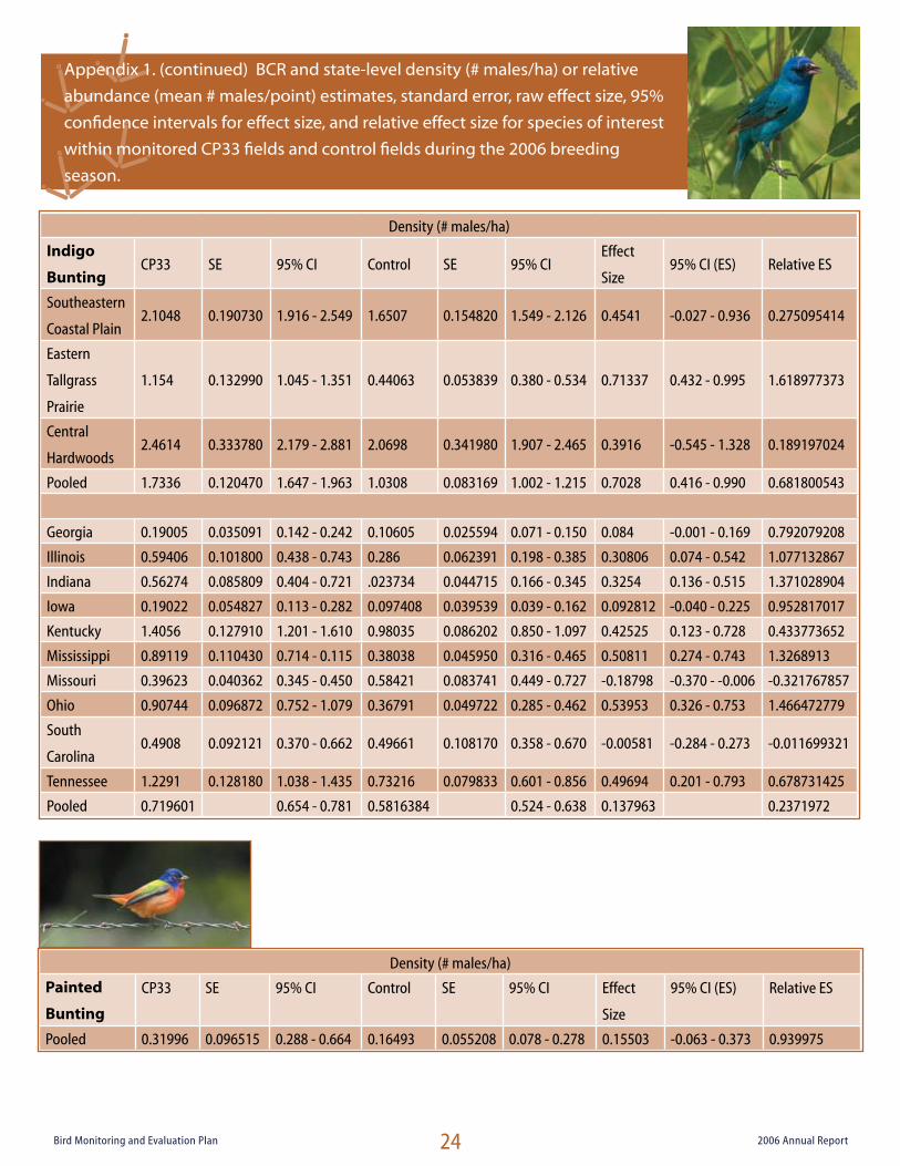
24Bird Monitoring and Evaluation Plan 2006 Annual Report
Density (# males/ha)
Indigo
BuntingCP33 SE 95% CI Control SE 95% CI
Effect
Size95% CI (ES) Relative ES
Southeastern
Coastal Plain2.1048 0.190730 1.916 - 2.549 1.6507 0.154820 1.549 - 2.126 0.4541 -0.027 - 0.936 0.275095414
Eastern
Tallgrass
Prairie
1.154 0.132990 1.045 - 1.351 0.44063 0.053839 0.380 - 0.534 0.71337 0.432 - 0.995 1.618977373
Central
Hardwoods2.4614 0.333780 2.179 - 2.881 2.0698 0.341980 1.907 - 2.465 0.3916 -0.545 - 1.328 0.189197024
Pooled 1.7336 0.120470 1.647 - 1.963 1.0308 0.083169 1.002 - 1.215 0.7028 0.416 - 0.990 0.681800543
Georgia 0.19005 0.035091 0.142 - 0.242 0.10605 0.025594 0.071 - 0.150 0.084 -0.001 - 0.169 0.792079208
Illinois 0.59406 0.101800 0.438 - 0.743 0.286 0.062391 0.198 - 0.385 0.30806 0.074 - 0.542 1.077132867
Indiana 0.56274 0.085809 0.404 - 0.721 .023734 0.044715 0.166 - 0.345 0.3254 0.136 - 0.515 1.371028904
Iowa 0.19022 0.054827 0.113 - 0.282 0.097408 0.039539 0.039 - 0.162 0.092812 -0.040 - 0.225 0.952817017
Kentucky 1.4056 0.127910 1.201 - 1.610 0.98035 0.086202 0.850 - 1.097 0.42525 0.123 - 0.728 0.433773652
Mississippi 0.89119 0.110430 0.714 - 0.115 0.38038 0.045950 0.316 - 0.465 0.50811 0.274 - 0.743 1.3268913
Missouri 0.39623 0.040362 0.345 - 0.450 0.58421 0.083741 0.449 - 0.727 -0.18798 -0.370 - -0.006 -0.321767857
Ohio 0.90744 0.096872 0.752 - 1.079 0.36791 0.049722 0.285 - 0.462 0.53953 0.326 - 0.753 1.466472779
South
Carolina0.4908 0.092121 0.370 - 0.662 0.49661 0.108170 0.358 - 0.670 -0.00581 -0.284 - 0.273 -0.011699321
Tennessee 1.2291 0.128180 1.038 - 1.435 0.73216 0.079833 0.601 - 0.856 0.49694 0.201 - 0.793 0.678731425
Pooled 0.719601 0.654 - 0.781 0.5816384 0.524 - 0.638 0.137963 0.2371972
Density (# males/ha)
Painted
Bunting
CP33 SE 95% CI Control SE 95% CI Effect
Size
95% CI (ES) Relative ES
Pooled 0.31996 0.096515 0.288 - 0.664 0.16493 0.055208 0.078 - 0.278 0.15503 -0.063 - 0.373 0.939975
Appendix 1. (continued) BCR and state-level density (# males/ha) or relative
abundance (mean # males/point) estimates, standard error, raw effect size, 95%
confidence intervals for effect size, and relative effect size for species of interest
within monitored CP33 fields and control fields during the 2006 breeding
season.
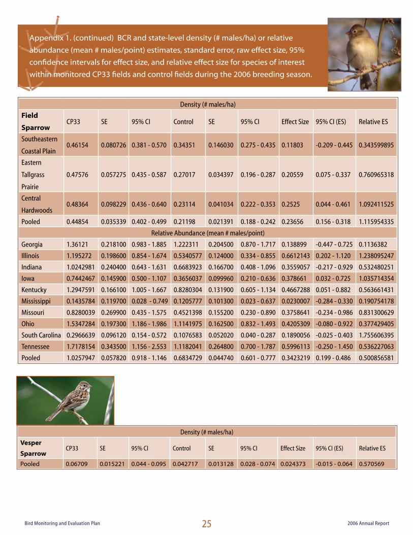
25Bird Monitoring and Evaluation Plan 2006 Annual Report
Density (# males/ha)
Field
SparrowCP33 SE 95% CI Control SE 95% CI Effect Size 95% CI (ES) Relative ES
Southeastern
Coastal Plain0.46154 0.080726 0.381 - 0.570 0.34351 0.146030 0.275 - 0.435 0.11803 -0.209 - 0.445 0.343599895
Eastern
Tallgrass
Prairie
0.47576 0.057275 0.435 - 0.587 0.27017 0.034397 0.196 - 0.287 0.20559 0.075 - 0.337 0.760965318
Central
Hardwoods0.48364 0.098229 0.436 - 0.640 0.23114 0.041034 0.222 - 0.353 0.2525 0.044 - 0.461 1.092411525
Pooled 0.44854 0.035339 0.402 - 0.499 0.21198 0.021391 0.188 - 0.242 0.23656 0.156 - 0.318 1.115954335
Relative Abundance (mean # males/point)
Georgia 1.36121 0.218100 0.983 - 1.885 1.222311 0.204500 0.870 - 1.717 0.138899 -0.447 - 0.725 0.1136382
Illinois 1.195272 0.198600 0.854 - 1.674 0.5340577 0.124000 0.334 - 0.855 0.6612143 0.202 - 1.120 1.238095247
Indiana 1.0242981 0.240400 0.643 - 1.631 0.6683923 0.166700 0.408 - 1.096 0.3559057 -0.217 - 0.929 0.532480251
Iowa 0.7442467 0.145900 0.500 - 1.107 0.3656037 0.099960 0.210 - 0.636 0.378661 0.032 - 0.725 1.035714354
Kentucky 1.2947591 0.166100 1.005 - 1.667 0.8280304 0.131900 0.605 - 1.134 0.4667288 0.051 - 0.882 0.563661431
Mississippi 0.1435784 0.119700 0.028 - 0.749 0.1205777 0.101300 0.023 - 0.637 0.0230007 -0.284 - 0.330 0.190754178
Missouri 0.8280039 0.269900 0.435 - 1.575 0.4521398 0.155200 0.230 - 0.890 0.3758641 -0.234 - 0.986 0.831300629
Ohio 1.5347284 0.197300 1.186 - 1.986 1.1141975 0.162500 0.832 - 1.493 0.4205309 -0.080 - 0.922 0.377429405
South Carolina 0.2966639 0.096120 0.154 - 0.572 0.1076583 0.052020 0.040 - 0.287 0.1890056 -0.025 - 0.403 1.755606395
Tennessee 1.7178154 0.343500 1.156 - 2.553 1.1182041 0.264800 0.700 - 1.787 0.5996113 -0.250 - 1.450 0.536227063
Pooled 1.0257947 0.057820 0.918 - 1.146 0.6834729 0.044740 0.601 - 0.777 0.3423219 0.199 - 0.486 0.500856581
Appendix 1. (continued) BCR and state-level density (# males/ha) or relative
abundance (mean # males/point) estimates, standard error, raw effect size, 95%
confidence intervals for effect size, and relative effect size for species of interest
within monitored CP33 fields and control fields during the 2006 breeding season.
Density (# males/ha)
Vesper
SparrowCP33 SE 95% CI Control SE 95% CI Effect Size 95% CI (ES) Relative ES
Pooled 0.06709 0.015221 0.044 - 0.095 0.042717 0.013128 0.028 - 0.074 0.024373 -0.015 - 0.064 0.570569

26Bird Monitoring and Evaluation Plan 2006 Annual Report
Density (# males/ha)
Eastern
KingbirdCP33 SE 95% CI Control SE 95% CI Effect Size 95% CI (ES) Relative ES
Pooled 0.097824 0.016409 0.085 - 0.142 0.10872 0.019095 0.253 - 0.425 -0.0109 -0.060 - 0.038 -0.10022
Relative Abundance (mean # males/point)
Southeastern
Coastal Plain0.2389091 0.041970 0.169 - 0.338 0.2006611 0.037770 0.138 - 0.291 0.038248 -0.072 - 0.149 0.190609939
Eastern
Tallgrass
Prairie
0.13067 0.026930 0.087 - 0.196 0.0686153 0.068620 0.040 - 0.118 0.0620548 -0.082 - 0.207 0.904387214
Central
Hardwoods0.1480813 0.052980 0.072 - 0.303 0.0888488 0.040520 0.036 - 0.222 0.0592325 -0.071 - 0.190 0.666666291
Georgia 0.1777406 0.072550 0.078 - 0.404 0.4062624 0.119300 0.224 - 0.738 -0.2285236 -0.502 - 0.045 -0.562499969
Illinois 0.2870823 0.092960 0.149 - 0.553 0.1435412 0.062270 0.060 - 0.346 0.1435411 -0.076 - 0.363 0.999999303
Indiana 0.0887031 0.038810 0.037 - 0.211 0.1428158 0.055360 0.066 - 0.308 -0.0541126 -0.187 - 0.078 -0.378897853
Iowa 0.3067465 0.094100 0.165 - 0.571 0.0894677 0.048720 0.030 - 0.270 0.2172788 0.010 - 0.425 2.428572546
Kentucky 0.1255536 0.043140 0.064 - 0.247 0.0534303 0.025780 0.021 - 0.138 0.0721232 -0.026 - 0.171 1.349855793
South
Carolina0.5610347 0.142100 0.336 - 0.973 0.2071605 0.073810 0.101 - 0.426 0.358742 0.040 - 0.667 1.708212714
Tennessee 0.1394139 0.076800 0.047 - 0.415 0.0627135 0.043490 0.016 - 0.248 0.0767003 -0.096 - 0.250 1.22302694
Pooled 0.1524523 0.019140 0.119 - 0.195 0.1065891 0.015570 0.080 - 0.142 0.0458632 -0.003 - 0.094 0.430280395
Appendix 1. (continued) BCR and state-level density (# males/ha) or relative
abundance (mean # males/point) estimates, standard error, raw effect size, 95%
confidence intervals for effect size, and relative effect size for species of interest
within monitored CP33 fields and control fields during the 2006 breeding season.
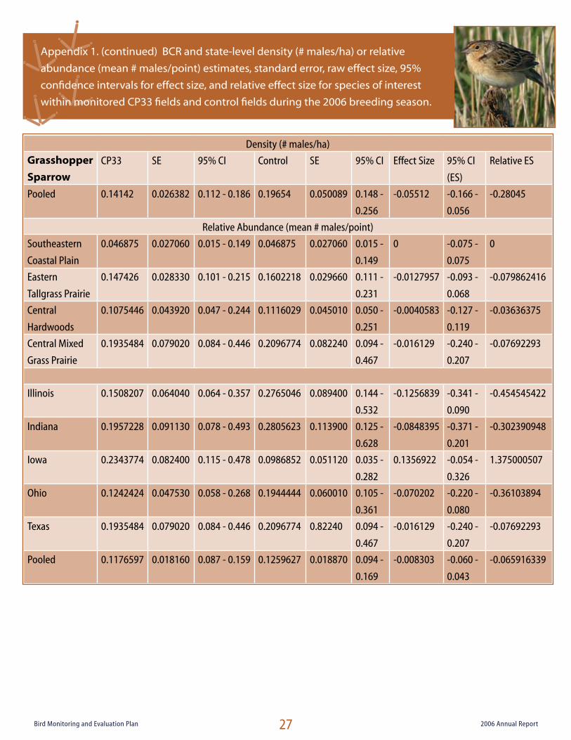
27Bird Monitoring and Evaluation Plan 2006 Annual Report
Density (# males/ha)
Grasshopper
Sparrow
CP33 SE 95% CI Control SE 95% CI Effect Size 95% CI
(ES)
Relative ES
Pooled 0.14142 0.026382 0.112 - 0.186 0.19654 0.050089 0.148 -
0.256
-0.05512 -0.166 -
0.056
-0.28045
Relative Abundance (mean # males/point)
Southeastern
Coastal Plain
0.046875 0.027060 0.015 - 0.149 0.046875 0.027060 0.015 -
0.149
0 -0.075 -
0.075
0
Eastern
Tallgrass Prairie
0.147426 0.028330 0.101 - 0.215 0.1602218 0.029660 0.111 -
0.231
-0.0127957 -0.093 -
0.068
-0.079862416
Central
Hardwoods
0.1075446 0.043920 0.047 - 0.244 0.1116029 0.045010 0.050 -
0.251
-0.0040583 -0.127 -
0.119
-0.03636375
Central Mixed
Grass Prairie
0.1935484 0.079020 0.084 - 0.446 0.2096774 0.082240 0.094 -
0.467
-0.016129 -0.240 -
0.207
-0.07692293
Illinois 0.1508207 0.064040 0.064 - 0.357 0.2765046 0.089400 0.144 -
0.532
-0.1256839 -0.341 -
0.090
-0.454545422
Indiana 0.1957228 0.091130 0.078 - 0.493 0.2805623 0.113900 0.125 -
0.628
-0.0848395 -0.371 -
0.201
-0.302390948
Iowa 0.2343774 0.082400 0.115 - 0.478 0.0986852 0.051120 0.035 -
0.282
0.1356922 -0.054 -
0.326
1.375000507
Ohio 0.1242424 0.047530 0.058 - 0.268 0.1944444 0.060010 0.105 -
0.361
-0.070202 -0.220 -
0.080
-0.36103894
Texas 0.1935484 0.079020 0.084 - 0.446 0.2096774 0.82240 0.094 -
0.467
-0.016129 -0.240 -
0.207
-0.07692293
Pooled 0.1176597 0.018160 0.087 - 0.159 0.1259627 0.018870 0.094 -
0.169
-0.008303 -0.060 -
0.043
-0.065916339
Appendix 1. (continued) BCR and state-level density (# males/ha) or relative
abundance (mean # males/point) estimates, standard error, raw effect size, 95%
confidence intervals for effect size, and relative effect size for species of interest
within monitored CP33 fields and control fields during the 2006 breeding season.

28Bird Monitoring and Evaluation Plan 2006 Annual Report
Density (# coveys/ha)
CP33 SE 95% CI Control SE 95% CI Effect Size95% CI
(ES)Relative ES
Southeastern
Coastal Plain0.035373 0.005210 0.031 - 0.047 0.016761 0.003210
0.014 -
0.0250.018512
0.007 -
0.0311.110434938
Eastern Tallgrass
Prairie0.033586 0.004710 0.027 - 0.045 0.017934 0.003538
0.015 -
0.0280.015652
0.004 -
0.0270.87275566
Central
Hardwoods0.031371 0.006551 0.023 - 0.046 0.033511 0.006627
0.027 -
0.051-0.00214
-0.020 -
0.016-0.063859628
Mississippi
Alluvial Valley0.018307 0.005777 0.012 - 0.032 0.0094458 0.004735
0.005 -
0.0170.0088612
-0.006 -
0.0240.938110059
Central Mixed
Grass Prairie0.27575 0.047957 0.241 - 0.355 0.23698 0.045317
0.190 -
0.3060.03877
-0.091 -
0.16800.163600304
Pooled 0.046998 0.003395 0.044 - 0.056 0.029511 0.0026730.029 -
0.0390.017487
0.009 -
0.0260.592558707
Arkansas 0.0053835 0.002220 0.002 - 0.011 0.011166 0.0079280.002 -
0.024-0.0057825
-0.022 -
0.010-0.517866738
Georgia 0.061364 0.013337 0.045 - 0.094 0.032155 0.0081160.024 -
0.0520.029209
-0.001 -
0.0600.908381278
Illinois 0.028855 0.009311 0.015 - 0.048 0.026286 0.0103830.011 -
0.0410.002569
-0.025 -
0.0300.097732633
Indiana 0.020612 0.006475 0.011 - 0.034 0.015354 0.0061000.009 -
0.0310.005258
-0.012 -
0.0230.342451478
Iowa 0.014826 0.006482 0.007 - 0.032 0.012114 0.0054050.004 -
0.0220.002712
-0.014 -
0.0190.223873205
Kentucky 0.011461 0.002907 0.007 - 0.020 0.026928 0.0066860.018 -
0.042-0.015467
-0.030 -
-0.001-0.574383541
Mississippi 0.046299 0.008192 0.036 - 0.061 0.013241 0.0036840.007 -
0.0200.033058
0.015 -
0.0512.496639227
Missouri 0.048303 0.006104 0.044 - 0.070 0.041281 0.0057990.037 -
0.0620.007022
-0.009 -
0.0240.170102468
Appendix 2. BCR and state-level density estimates (# coveys/ha), 95% bootstrap confidence intervals
(B=1000), and raw and relative effect sizes for calling bobwhite coveys within monitored CP33 fields
and control fields during the 2006 fall of 2006 and BCR and state-level density estimates adjusted
for number of adjacent calling coveys, % cloud cover, wind speed, and 6-hr change in barometric
pressure (Wellendorf et al. 2004). 95% confidence intervals on effect size were included for
unadjusted density estimates.
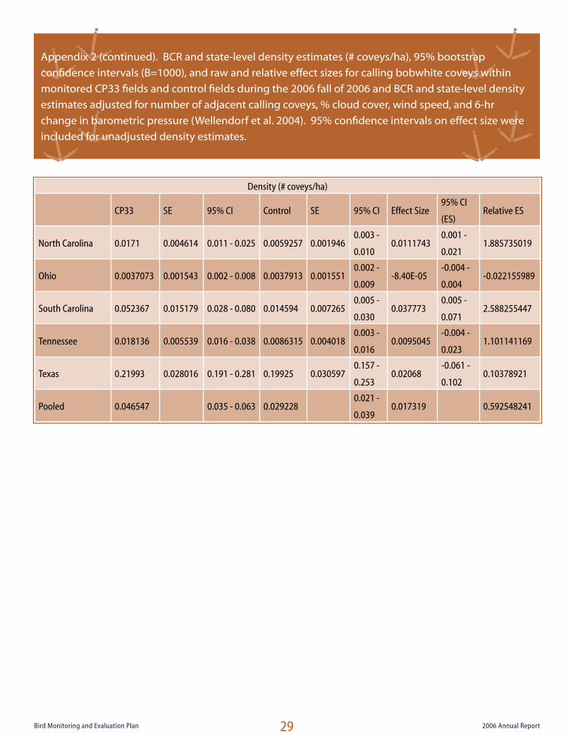
29Bird Monitoring and Evaluation Plan 2006 Annual Report
Density (# coveys/ha)
CP33 SE 95% CI Control SE 95% CI Effect Size95% CI
(ES)Relative ES
North Carolina 0.0171 0.004614 0.011 - 0.025 0.0059257 0.0019460.003 -
0.0100.0111743
0.001 -
0.0211.885735019
Ohio 0.0037073 0.001543 0.002 - 0.008 0.0037913 0.0015510.002 -
0.009-8.40E-05
-0.004 -
0.004-0.022155989
South Carolina 0.052367 0.015179 0.028 - 0.080 0.014594 0.0072650.005 -
0.0300.037773
0.005 -
0.0712.588255447
Tennessee 0.018136 0.005539 0.016 - 0.038 0.0086315 0.0040180.003 -
0.0160.0095045
-0.004 -
0.0231.101141169
Texas 0.21993 0.028016 0.191 - 0.281 0.19925 0.0305970.157 -
0.2530.02068
-0.061 -
0.1020.10378921
Pooled 0.046547 0.035 - 0.063 0.0292280.021 -
0.0390.017319 0.592548241
Appendix 2 (continued). BCR and state-level density estimates (# coveys/ha), 95% bootstrap
confidence intervals (B=1000), and raw and relative effect sizes for calling bobwhite coveys within
monitored CP33 fields and control fields during the 2006 fall of 2006 and BCR and state-level density
estimates adjusted for number of adjacent calling coveys, % cloud cover, wind speed, and 6-hr
change in barometric pressure (Wellendorf et al. 2004). 95% confidence intervals on effect size were
included for unadjusted density estimates.
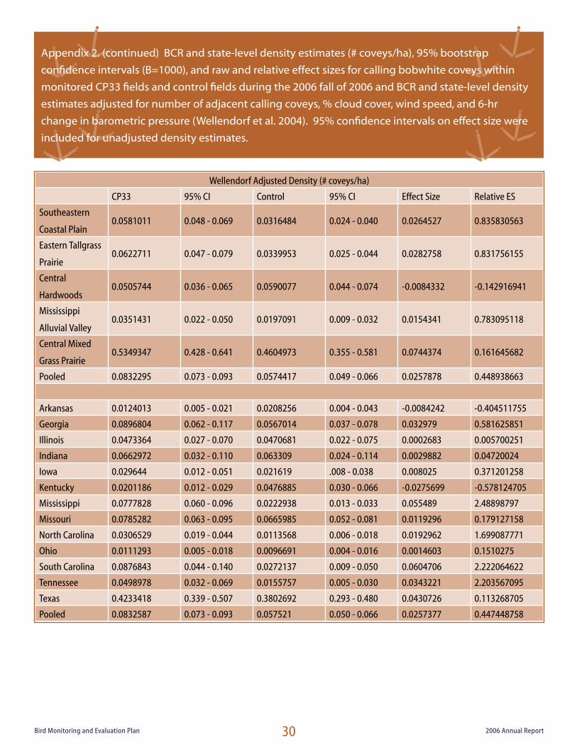
30Bird Monitoring and Evaluation Plan 2006 Annual Report
Appendix 2. (continued) BCR and state-level density estimates (# coveys/ha), 95% bootstrap
confidence intervals (B=1000), and raw and relative effect sizes for calling bobwhite coveys within
monitored CP33 fields and control fields during the 2006 fall of 2006 and BCR and state-level density
estimates adjusted for number of adjacent calling coveys, % cloud cover, wind speed, and 6-hr
change in barometric pressure (Wellendorf et al. 2004). 95% confidence intervals on effect size were
included for unadjusted density estimates.
Wellendorf Adjusted Density (# coveys/ha)
CP33 95% CI Control 95% CI Effect Size Relative ES
Southeastern
Coastal Plain0.0581011 0.048 - 0.069 0.0316484 0.024 - 0.040 0.0264527 0.835830563
Eastern Tallgrass
Prairie0.0622711 0.047 - 0.079 0.0339953 0.025 - 0.044 0.0282758 0.831756155
Central
Hardwoods0.0505744 0.036 - 0.065 0.0590077 0.044 - 0.074 -0.0084332 -0.142916941
Mississippi
Alluvial Valley0.0351431 0.022 - 0.050 0.0197091 0.009 - 0.032 0.0154341 0.783095118
Central Mixed
Grass Prairie0.5349347 0.428 - 0.641 0.4604973 0.355 - 0.581 0.0744374 0.161645682
Pooled 0.0832295 0.073 - 0.093 0.0574417 0.049 - 0.066 0.0257878 0.448938663
Arkansas 0.0124013 0.005 - 0.021 0.0208256 0.004 - 0.043 -0.0084242 -0.404511755
Georgia 0.0896804 0.062 - 0.117 0.0567014 0.037 - 0.078 0.032979 0.581625851
Illinois 0.0473364 0.027 - 0.070 0.0470681 0.022 - 0.075 0.0002683 0.005700251
Indiana 0.0662972 0.032 - 0.110 0.063309 0.024 - 0.114 0.0029882 0.04720024
Iowa 0.029644 0.012 - 0.051 0.021619 .008 - 0.038 0.008025 0.371201258
Kentucky 0.0201186 0.012 - 0.029 0.0476885 0.030 - 0.066 -0.0275699 -0.578124705
Mississippi 0.0777828 0.060 - 0.096 0.0222938 0.013 - 0.033 0.055489 2.48898797
Missouri 0.0785282 0.063 - 0.095 0.0665985 0.052 - 0.081 0.0119296 0.179127158
North Carolina 0.0306529 0.019 - 0.044 0.0113568 0.006 - 0.018 0.0192962 1.699087771
Ohio 0.0111293 0.005 - 0.018 0.0096691 0.004 - 0.016 0.0014603 0.1510275
South Carolina 0.0876843 0.044 - 0.140 0.0272137 0.009 - 0.050 0.0604706 2.222064622
Tennessee 0.0498978 0.032 - 0.069 0.0155757 0.005 - 0.030 0.0343221 2.203567095
Texas 0.4233418 0.339 - 0.507 0.3802692 0.293 - 0.480 0.0430726 0.113268705
Pooled 0.0832587 0.073 - 0.093 0.057521 0.050 - 0.066 0.0257377 0.447448758