Research Division Federal Reserve Bank of St. Louis Working Paper Series

Connectionist-Based Rules Describing the Pass-through of Individual Goods Prices into

Trend Inflation in the United States

Richard G. Anderson Jane M. Binner

and Vincent A. Schmidt

Working Paper 2011-007A http://research.stlouisfed.org/wp/2011/2011-007.pdf

February 2011

FEDERAL RESERVE BANK OF ST. LOUIS

Research Division P.O. Box 442

St. Louis, MO 63166

______________________________________________________________________________________

The views expressed are those of the individual authors and do not necessarily reflect official positions of the Federal Reserve Bank of St. Louis, the Federal Reserve System, or the Board of Governors.

Federal Reserve Bank of St. Louis Working Papers are preliminary materials circulated to stimulate discussion and critical comment. References in publications to Federal Reserve Bank of St. Louis Working Papers (other than an acknowledgment that the writer has had access to unpublished material) should be cleared with the author or authors.

1

Connectionist-Based Rules Describing the Pass-through of Individual Goods Prices into

Trend Inflation in the United States

Richard G. Anderson a, b

Jane M. Binner b

Vincent A. Schmidt c

a Federal Reserve Bank of St. Louis

b University of Sheffield, School of Management

c U.S. Air Force Research Laboratory, Dayton, Ohio

February 2011

Keywords: Consumer prices, Inflation, Neural Network, Data Mining, Rule Generation

JEL Codes: E31, C45

Views expressed herein are solely those of the authors, and are not necessarily the views

of the Federal Reserve Bank of St Louis or the Federal Reserve System. Paper cleared

by the Department of Defense for public release #88ABW-2010-1111. Anderson thanks

the Aston Business School, Aston University (Birmingham UK) and the Management

School, Sheffield University (Sheffield UK) for financial support and hospitality during

the conduct of this research. Anderson also thanks the Research Division of the Federal

Reserve Bank of Minneapolis for hospitality during the completion of this manuscript.

The authors thank Yang Liu of the Federal Reserve Bank of St. Louis for research

assistance.

2

Abstract

This paper examines the inflation "pass-through" problem in American monetary policy,

defined as the relationship between changes in the growth rates of individual goods and

the subsequent economy-wide rate of growth of consumer prices. Granger causality tests

robust to structural breaks are used to establish initial relationships. Then, a

feedforward artificial neural network (ANN) is used to approximate the functional

relationship between selected component subindexes and the headline CPI. Moving

beyond the ANN “black box,” we illustrate how decision rules can be extracted from the

network. Our custom decompositional extraction algorithm generates rules in human-

readable and machine-executable form (Matlab code). Our procedure provides an

additional route, beyond direct Bayesian estimation, for empirical econometric

relationships to be embedded in DSGE models. A topic for further research is

embedding decision rules within such models.

3

Introduction

This is a study in data mining, and also a study in macroeconomics. We apply a

nonparametric, nonstructural, connectionist model (artificial neural network, or ANN)

to examine the “inflation pass-through problem,” that is, how large (if any) is the

subsequent change in the headline or core (excluding food and energy) inflation rate

following an abrupt increase or decrease in the rate of change of the price of a specific

commodity or group of commodities. Following the connectionist paradigm, we extract

sets of “human readable” rules that span the same mapping as the underlying network

from inputs to outputs. We suggest that such tools are potentially useful in economics.

This analysis thus both presents some evidence regarding inflation pass-through and

illustrates the power and value of interpreting neural networks in terms of rules rather

than as black box forecasting tools.

Data mining is a broad term describing the use of statistical methods to locate

interesting and (usually) less-than-obvious relationships among variables. Traditional

data mining relies on classification and association rules: it has been described as “a

cooperative effort of humans and computers” (Weiss and Indurkhya, 1998) and as “the

automatic extraction of novel, useful and understandable patterns in very large

databases" (Zaki, 1998). Often, it is a computationally intensive task that includes

experimentation over a range of models.

Data mining, the mystical art of calling forth hordes of applicable, relevant marketable knowledge from both small, limited, contemporary surveys and from databases teeming with years of facts alike... and neurocomputing, the arcane magic of coaching case after case of information through a winding series of artificial neurons, breathing life into the ever-changing, constantly rearranging connectionist web, ever searching for the perfect match between sensory input and perceived reality. Combine these mighty forces and gain the ultimate prize – or, perhaps, complete chaos (most likely). The magic of these models is a very satisfying illusion but there is substantial mathematical power in each one...if it can be harnessed correctly. -- Schmidt (2002)

4

Connectionist Neural Networks

The descriptive term “connectionist” was introduced by Feldman and Ballard

(1982) to describe an emphasis on the use of neural networks as statistical tools, with

little (if any) reference to biology or human physiology.1 The popularity of

connectionist models as statistical tools in economics dates largely from the studies by

Hal White and collaborators (Hornick, Stinchcombe and White, 1989, 1990; White,

1988, 1989, 1990; Kuan and White, 1994). Hornick et al (1989), for example, established

that a feedforward neural network with one hidden layer is able to approximate an

unknown continuous real-valued function to an arbitrary level of accuracy (e.g., Judd,

1998, pp 245-6). Other studies have proven that feedforward networks with a single

hidden layer can perform classification for decision regions that are not convex. White

(1990) provided conditions under which the least-squares (or maximum likelihood)

estimation of feedforward networks is statistically consistent. Recent papers concerning

inflation include Binner et al (2010) and Nakumura (2005); McNelis (2005) and Blynski

and Faseruk (2006) discuss the use of neural networks in financial economics; Lim and

McNelis (2008) use neural networks to approximate complex first-order conditions in

solving DSGE macroeconomic models.; and recent forecasting papers include Pradhan

and Kumer (2008) and Kiani and Kastens (2008). 2 A second thread of the connectionist

literature, exemplified by early research in Australia (Andrews et, 1995) and at the

1. Stephen Gallant also was an early supporter of the connectionist viewpoint (Gallant, 1988, 1993).

Medler (1998) surveys the history of connectionist thought; see also Cheng and Titterington (1994).

2. Despite classic articles cautioning users that neural networks are not to be treated as a “black box”

with mystical and magical powers (Sarle, 1994; Faraway and Chatfield, 1998), extraordinary (and false)

claims continue to appear in print. For example, Yildiz and Yezegel (2010) claim: “The most powerful

feature of artificial neural network technology is solving nonlinear problems that other classical techniques

do not deal with. The artificial neural network (ANN) technology does not require any assumption about

data distribution and missing, noisy and inconsistent data do not possess any problems. Another

important aspect of the ANN is its ability to learn from the data. Artificial neural network technology is

used in classification, clustering, predicting, forecasting, pattern recognition problems successfully. In most

cases, ANN technology produces superior performance than other statistical techniques.” Persons familiar

with the methods will immediately recognize this as false. Other published papers include mistreatment of

the methods that are obvious to the better informed—Haider and Hanif (2009) estimate a network with

12 hidden layers.

5

University of Wisconsin (e.g., Towell and Shavlik, 1993), is the extraction of human-

readable rules from the model, so that that the model need not be considered an

impenetrable “black box.” In its most comprehensive form, such a set of rules provides

the same mapping from inputs to outputs as is provided by the connectionist model

(ANN) itself. Connectionist models and the extracted rules are members of the family of

statistical tools referred to as “hybrid systems,” including fuzzy-logic-based systems.

The essential “fuzziness” of fuzzy logic systems is an emphasis on inference while

acknowledging that “structural” information is incomplete or imprecise. Robustness is

critical. Constraints (usually exogenously imposed) prevent the system’s extracted rules

from suggesting unreasonable choices. The term “fuzzy” does not imply “uncertain”,

“inaccurate” or “confused” systems, but rather describes systems that rely on a

mathematical foundation that seeks to capture concepts such as of "mostly", “rarely",

“often”, “white but not quite white”, “white or black”, and “black but not quite black”.

Fuzzy inference is closely connected to the literature on model robustness in which rules

extracted from models, including those extracted from macroeconomic models, usually

are best interpreted as highly uncertain, with a premium on robustness (e.g, Orphanides

and Williams, 2003, 2007).

The Inflation Pass-Through Problem

Simply stated, the pass-through problem asks whether future values of a headline

or “core” (that is, excluding food and energy) inflation rate will be affected by current

or earlier period changes in the rate of increase/decrease in certain other prices. Usually,

the most volatile prices are chosen for study, often food and energy prices.

Models of inflation pass-through, and indeed all inflation forecasting models,

must acknowledge the inflation targeting regime of the monetary authorities (Bernanke,

Gertler and Watson, 1997). Inflation pass-through is likely to be small when the

authorities have credibility regarding policy implementation and have adopted an

inflation target. In the extreme case of “inflation nutters,” there will be little or no pass-

through if there exist a set of policy actions capable of preventing it. For more moderate

policymakers operating in a sticky price (slowing changing expectations) environment,

some near-term pass-through might be permitted so as to temper any downward

6

pressure on economic activity emanating from anti-inflationary policies. 3 Reduced-form

studies of the type in this analysis are of value when there is no agreed upon general

equilibrium model for policymaking and evaluation, and when the dates of putative

changes in inflation regimes and/or policymakers distaste for inflation are highly

uncertain. The relationships that link movements in individual prices to the aggregate

inflation trend are difficult to estimate because they depend on the private sector’s

perception of policymakers’ time-varying inflation goals and strength of commitment to

low, stable inflation. Changes in a nation's political leadership may refocus concern on

price stability versus more rapid growth of economic activity. 4

In recent years the relationship between changes in the prices of individual goods

and services and overall consumer inflation has assumed prominence in academic

literature and in central banks' circles. Some central bankers explicitly have accepted

that subsets of consumer prices are the appropriate objectives of monetary policy (core

measures excluding food and energy prices), while others prefer overall "headline"

inflation as a target. The most prominent among the former is the U.S. Federal Reserve,

which has accepted the core chain price index for personal consumption expenditures

("core PCE") as its policy objective. Among the latter are the Bank of England and the

European Central Bank, which prefer the headline measure because it includes all the

products purchased by consumers, including food and energy.

In addition, the pattern of price increases across goods and services changes

through time. The pattern of external shocks (such as weather patterns and energy

prices) affecting the economy varies, as do the levels of economic activity in trading

partner countries. Further, the (endogenous) reaction of firms and households may differ

among goods, with some price changes eliciting strong reactions and others little if any

reaction. Such variation will affect the strength and pattern of pass through from

changes in individual prices to the overall headline inflation rate.

Energy prices often are regarded as the most likely to have large pass through

effects because changes in energy prices are quickly observed by households and firms:

energy products are purchased more-or-less continuously. Further, energy is an essential

3. See for example Gagnon and Ihrig (2004), Mishkin and Schmidt-Hebbel (2001, 2006).

4. For models of the latter type, see Owyang and Ramey (2004) and Francis and Owyang (2005).

7

input to transport, although only one of a number of inputs. The actions of households

and firms will tend to temper other goods’ price movements. Prices of consumer durable

goods, such as cars and home furnishings, are expected to have the weakest pass

through because these purchases are more readily deferred. Intermediate are prices for

foods because less expensive food products may be substituted when prices increase

sharply.

Our work is related to the large literature on the recessionary effects of oil price

shocks, including Hamilton (2003, 2009), Hamilton and Herrera (2004), Hooker (1996),

Barsky and Kilian (2001), Segal (2007), Norhaus (2007), Kilian (2008), and Blanchard

and Riggi (2009). Studies specifically addressing the passthrough problem include

Hooker (2002), van den Noord and Andre (2007), De Gregorio, Landerretche, and

Neilson (2007), Cecchetti et al (2007), Blanchard and Gali (2008), Chen (2009), and

Clark and Terry (2010). The latter group of studies, like the former, has focused on oil

and has found little passthrough since the mid-1980s. Reasons cited include more

flexible foreign exchange markets, more active monetary policy, and a higher degree of

trade openness, although the evidence (with the recent exception of Clark and Terry’s

Bayesian VAR containing time-varying coefficients and variances) has largely relied on

relatively simple methods of assessing changes over time. Broadly, the literature has

concluded that: (i) the relationship between oil prices and economic activity has been

time-varying, with changes in both regression coefficients and innovation variances; (ii)

the relationship likely was nonlinear, with sharp price increases adversely affecting

economic activity far more than price decreases boosted activity (if they did so at all);

(iii) an almost-sure structural break occurred between the second year of Paul Volcker’s

disinflation policy (circa 1981) and the collapse of oil prices in 1985-86, and (iv) the

sharp decrease in the sensitivity of economic activity and inflation to oil prices after

1985 almost surely reflected both a more sophisticated public understanding of the

volatility of oil prices and a Federal Reserve that, by committing itself to low, stable

inflation, felt itself less compelled to respond to adverse supply shocks. Moving beyond

oil, this study more broadly explores housing, food, and transportation prices, as well as

a broader energy price index.

8

Empirical Analysis of Passthrough

We present here an empirical summary of the relationship between individual-

component price indexes and the headline inflation rate (in the CPI-U-RS data). We

focus on prices indexes for four important subgroups: housing, transport, energy and

food. Housing expenditures, by itself, comprises 40 percent of expenditures in the overall

headline index, and more than half of the expenditures in the “core” index (excluding-

food-and-energy). We focus on quasi-reduced-form relationships between “causal” and

output variables, following in style, for example, Chen, Rogoff and Rossi (2010).

Our data are the Bureau of Labor Statistics’s Consumer Price Index “Research

Series” (CPI-U-RS) in which indexes have been constructed for historical dates using

the same definitions and methods used for newly published data (Stewart, 1998).5 We

include the aggregate “headline” index, a “core” index (excluding food and energy

prices), and subcomponent indexes for food, energy, housing, and transportation. Our

figures are the monthly percentage change from the same month one year earlier, not-

seasonally-adjusted, from December 1977 through December 2009.6

We ask if any of the four component indexes (food, energy, housing, transport)

Granger-causes (GC) either the headline or core index. Such tests are well-known to

lack robustness to structural breaks. Rossi (2005) considers the case when a subset of

parameters is to be tested against a known alternative while admitting the possibility of

parameter instability, and derives a family of optimal (locally asymptotically most

powerful) tests. Here, we use the simplest computational form of the test, as in Chen,

5 We sometimes have been asked to explain the difference between the CPI-U and CPI-U-RS series. The

principal difference is the treatment of housing and mortgage interest during 1977-1983 when the CPI-U

increases and later decreases more rapidly than the CPI-U-RS. Measured year-over-year, the CPI-U-RS

exceeded 10 percent per annum from September 1979 to March 1981, peaking in March 1980 at 11.8

percent. In contrast, the CPI-U exceeded 10 percent from March 1979 to April 1981, peaking in April

1980 at 14.7 percent. The CPI-U thereafter fell to a low of 2.5 percent in June 1983, when the CPI-U-RS

was at 4.3 percent. The low point for the CPI-U-RS was December 1983 at 3.8 percent, a month in which

the CPI-U also was 3.8 percent. 6 Year-over-year measures remove the necessity for modeling seasonal effects, and specifically avoids the

well-known lead-lag distortions that are present in data seasonally adjusted using the two-sided filters in

the Census X-11/X-12 program. In this study, approximately the same results are obtained using data

pre-filtered using monthly dummy variables.

9

Rogoff and Rossi (2010). Let the parameter vector be partitioned as 1 2, ,

denote a partition of the sample 1 1, ..., , , ...,T T T , J the distribution function of ,

s denote the time-position of an observation within the sample, and 1s be the

indicator function that equals unity if s T and zero otherwise. For the null hypothesis

2* and the alternative 2 1 1*

A sT T ,

Rossi (equ 23, 24) shows that, for a particular Gaussian weighting function, the

test statistic with the greatest average power has the asymptotic distribution

121

*expc

dJc

1 11

* ''p p

p p

BB BBB B

where p is the number of parameters not specified under the null, B is scalar

Brownian motion, and BB is a p-dimensional Brownian bridge. The specific statistic

we consider is the Andrews-Quandt optimal test, *TQLR , which is obtained by allowing

1c c and has asymptotic distribution *sup T

(Rossi, equ (27)). The statistic

*T may be computed in alternative asymptotically equivalent forms. We choose the

Lagrange multiplier form as used, for example, in Chen, Rogoff, and Rossi (2010),

1 2*T LM LM , where 1LM corresponds to 2 2

* and 2LM corresponds to the

Andrews QLR test for a break at an unknown breakpoint, say, T (Rossi, equ (23)).

Tables 1, 2 and 3, respectively, report p-values for Granger causality (GC), Andrews

QLR, and Rossi’s optimal tests. The sections labeled “Panel A” correspond to the

headline and core CPI as the dependent variable and the component subindexes as the

explanatory variable, while the sections labeled “Panel B” correspond to tests of

feedback (“reverse causation”) with the subindexes as dependent variables and headline

or core as the explanatory variable.

We conducted extensive lag-length selection experiments for all 6 price indexes,

using AIC, BIC and a general-to-specific strategy, each beginning with a length of 40

periods. Our experiments suggest that it is essential to begin with a large putative lag:

beginning with a software-default of six periods, all three tests suggested a lag of one

period, that is, suggested writing the regressions in the “predictive form”

,t t r t r ty f y x with 1r , regardless of whether the data were monthly month-to-

10

month or year-over-year percentage increases. Beginning at 40 periods, the AIC and

BIC selected lag lengths of 12 and 24 periods, respectively, for both month-to-month

and year-over-year changes. For robustness, the tables display results for lag lengths of

13 and 25 periods. The data are year-over-year percentage changes, monthly.

Consider first the upper half of table 1, for headline CPI. The results in panel A

reject the null that the headline CPI is not Granger caused by energy, transport, and

housing at both lag lengths, and by food at the longer lag. The reverse-causality results

in panel B reject the null that the headline CPI is not GC by transport, housing and

food at the shorter lag length, and transport and housing at the longer lag. The

combined direct and reverse causality results for the housing price index suggest

simultaneity between the headline and housing index, perhaps due to imputed items. In

the lower half of table 1, for core inflation, the direct-causality results in panel A

suggest rejecting the null of no GC only for food at the shorter lag. The reverse-

causality results in panel B suggest rejection only for housing and food, at the shorter

lag.

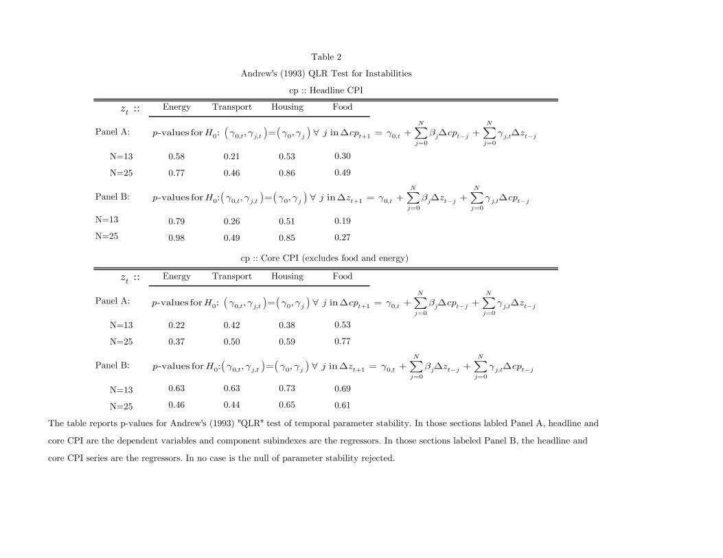
Table 2 reports Andrews QLR tests. The tests fail to reject the null of parameter

stability for all series and both lag lengths. Note that in each regression only a subset of

the parameters (those on the “explanatory” variable) are time-varying under the

alternative. Although surprising at first, it must be kept in mind that CPI-U-RS data,

as a constant methodology series, are somewhat smoother than the CPI-U data,

especially during the late 1970s and early 1980s. Previous studies that have identified

breaks circa the mid-1980s (e.g., Clark and Terry, 2011) often have used quarterly data

and considered data earlier than the 1977 beginning of the CPI-U-RS series. 7

Table 3 reports p-values for Rossi’s (2005) robust tests. We include these tests for

completeness despite the Andrews QLR test showing no breaks. Where possible, p-

values are linearly interpolated between the asymptotic critical values in Rossi (2005),

table B.3, p. 990. Where test statistics fall outside the bounds of her table, the p-values

are denoted “<0.01” or “>0.10”. Both direct GC (panel A) and reverse GC (panel B)

is reported. In the upper half of Table 3 for headline CPI and direct causality (panel A),

7 The Bureau of Labor Statistics also has published a CPI-U-X1 series for dates beginning 1967. Because

its methodology differs somewhat from the CPI-U-RS, we do not include it here.

11

we reject at the 10 percent level the null of no GC by energy, transport and housing at

both lag lengths, and for food at the 5 percent level for the longer lag. In panel B

(reverse causality), we reject at the 5 percent level the null of no GC for transport,

housing and food at the shorter lag, and for housing at the longer lag. Inference

regarding housing continues to be clouded by strong reverse GC. In the lower half of

Table 3 for core CPI, in panel A, the null of no GC is rejected for energy, housing and

food at the shorter lag length; in panel B (reverse causality), the null is rejected for

housing and food at the shorter lag.

The above tests suggest that the relationships between headline and core CPI,

and the energy and transport component subindexes, are sufficiently reliable to warrant

further exploration. Food prices also have support, but due to the results sensitivity to

lag length we leave them as a topic for future research.

Technical Details Regarding Neural Network

A comprehensive discussion of connectionist models is beyond the scope of this

paper. To make the paper more self-contained, however, we include here a brief

summary of connectionist models from a statistical point of view. The discussion follows

Bishop (1995), who described the artificial neural network (ANN) as a “general

parameterized nonlinear mapping between a set of input variables and a set of output

variables.” Given a sufficient number of terms, the ANN can approximate any

reasonable function to arbitrary accuracy.

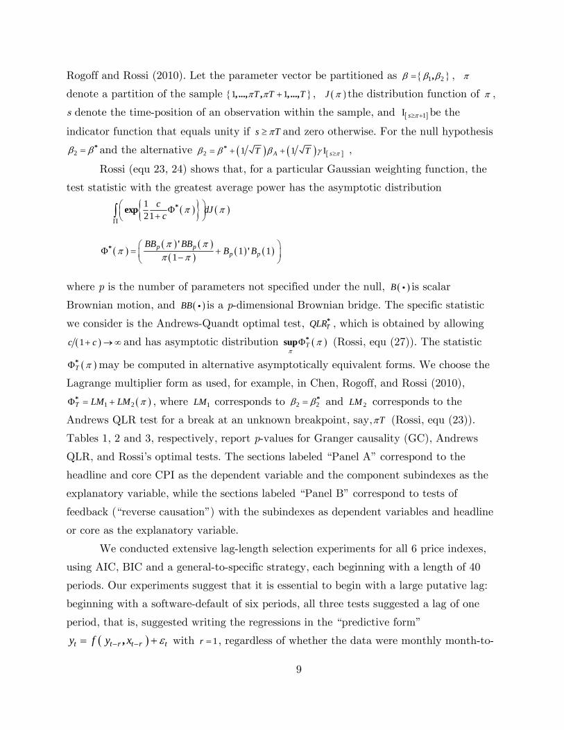
The multi-layer connectionist network may be expressed as a convolution

(superposition) of functions. Recall that a two-layer feedforward network (one hidden

layer plus one output layer) is sufficient to approximate any reasonable unknown

function to any arbitrary degree of accuracy (Hornik et al, 1989). Consider a network

with d input nodes, M hidden units, and c output units. The output of the j-th

hidden unit, ja , is the linear function

(1) (1), ,0

1

d

j j t i ji

a w x w

12

where the ix are inputs and the (1) (1), ,0,j t jw w are coefficients (“weights”) to be determined

during network “training.” 8 The importance of the j-th hidden layer is determined by

its activation function, ( )jg a . Activation functions are binary functions, the two most

popular being the Heaviside step function

0 0

( )1 0

ag a

a

and the continuous sigmoidal function

1

( )1 a

g ae

.

In turn, the k-th network output may be expressed as

(2) (2), ,0

1

( )M

k jk j kj

y w g a w

Often in economics k=1, that is, there is a single output.

An additional issue in economics is that the networks often are treated as black

boxes, where the analyst may be unconcerned with the internal workings of the

network—that is, the estimated weights and choice of functions (e.g., Swanson and

White, 1995, 2007). It is well-known, however, that such practice is dangerous; attention

must be paid to the structure of the network even if (or, perhaps, particularly if) it is

identified and estimated “automatically” during the training phase (e.g., Sarle, 1994;

Faraway and Chatfield, 1998). One technique for doing so is rule extraction from the

network (e.g., Baesens et al., 2003).

Model Estimation (Training)

In terms used by neural network scientists, our connectionist model is a

“supervised three-layer feedforward neural network, using sigmoidal activation functions

and linear output functions, trained via back propogation.” (It is “supervised” because

the training includes both inputs and outputs; it has three layers because there are

input, hidden, and output layers.) Training (that is, estimation) of such models is a

mixed integer-real optimization problem involving choosing the number of nodes in the

8 Here we include explicit additive “bias” terms 1

0( ),jw . These may be subsumed into the weights 1( )

,j tw by

appending a vector of ones to the jx .

13

hidden layer and estimation of the network’s weights.9 We conducted a grid search with

respect to the integer, examining models with 2, 3, 4, 5, 6, 7, 8, 9, and 12 nodes in the

single hidden layer. For all networks, the single hidden layer applied a sigmoid

activation function (MATLAB's logsig function), and an unconstrained linear link

function (MATLAB's purelin function) was used for the six nodes at the output layer.

All candidate models were provided the same dataset. The estimation/training dataset

contained 242 observations and the test dataset contained 131 observations, both groups

randomly selected from a set of 343 monthly observations. All networks were trained for

2500 epochs, and for each architecture the single best of 25 instances was chosen for

evaluation.10 Note that the “best” network instance was defined as the instance with the

highest training and testing accuracy.11

9 For neural networks, “training” is the process of iteratively determining the number of hidden

(intermediate) layers and estimating the weights (conditional on the choice of activation function).

Available data are divided into a training set, a test set, and a validation set. Training algorithms

typically iterate through the training dataset, with the test and validation datasets used to avoid

accepting a network that has been overfitted during training. 10 An epoch is one backward and forward pass through the dataset, creating a set of values for the

weights. The number of epochs is the number of iterations through the data. Typically, several thousand

iterations are necessary to achieve the a prior minimum acceptable degree of fit to the data (essentially,

the maximum permitted sum of squared residuals). An excessive number of nodes and/or iterations risks

overfitting in-sample, and subsequent poor forecasting performance. Protection against overfitting is

achieved by examining the model’s error when subsequently confronted with the hold-out datasets (the

test and validation datasets). 11 Although 25 network instances were trained, solutions tend to fall into small numbers of "classes" or

"categories." In this case, the “best” network is merely a (reasonably) random selection of a single solution

from the category of networks exhibiting the most desirable behavior. Any network instance within this

class would be a suitable selection (candidate) for the rule extraction. The main difference across

instances is the set of starting values for estimation of the weights, which are chosen randomly; algorithms

for the optimal choice of starting values is a topic of current research in the neural network field (see

Sulaiman et al, 2005; Asadi et al, 2009). Also, we are merely using the network to discover and describe

relationships within the data. The “real” product of our exercise are the rules generated via the extraction

algorithm; these rules are an approximate representation of the neural network. The extraction process

and the focus on the rules decouples at least in part the end result from the specific details of the

network.

14

To date, all algorithms for ANN rule extraction require that data be discretized

prior to network training. 12 One common technique is two-step “thermometer

encoding.” First, the continuous data are recoded as if they were values falling in a set

of discrete intervals. Second, these discrete values are encoded into a thermometer-like

array of (typically) Boolean values. 13 This technique is illustrated in Figure 1, using all-

items headline CPI. As illustrated in the upper panel, N-1 thermometer variables (T1 to

T5) are required to encode a series that has been discretized into N ranges. The lower

panel displays the encoding for selected dates. Note that this example also highlights the

major shortcoming that limits the use of rule-based connectionist models in economics:

all time-series information is lost in such encoding.14

Selection of ranges for all variables was assisted by the automated clustering

algorithm of Schmidt (2002). Transportation and energy were classified into 12 and 17

bins, respectively. The same algorithm was initially used to cluster the inflation values,

but inspection of the values and a comparative test at selected breakpoints resulted in

headline inflation being manually discretized into six ranges. After encoding, the model

has 29 (12 + 17) inputs and six outputs, as shown in Table 4.

Our preference is to accept the most accurate model that also has the smallest

number of nodes in the single hidden layer because doing so reduces the combinatorial

complexity of rule extraction. Interestingly, all tested networks—including those with

only 2 nodes in the hidden layer—produced accuracy in the range of 87%-89% for

training data, and 82%-84% for testing data. Eventually, we chose a model with five

12 A little-known exception is Setiono et al (2002) who extracts rules by approximating hidden node

activation functions by piecewise linear functions. Exploration of their methods is left as a topic for future

research. 13 This discretization is less restrictive in the connectionist model than is occasionally argued. Rules

obtained from the ANN’s output typically are of the if-then-else form plus constraints and often have

ranges wherein the optimal action is to take no action whatsoever. This suggests that an economic model

of costs and benefits should underlie the discretization process, a topic beyond the scope of this paper but

essential if ANN-based rules eventually are to be embedded in DSGE macro models. 14 Dynamic models can be constructed by using a two-dimension set of ranges such that each observation

is encoded based on the value during period t and the value during period t-1.So doing in this example

would double the number of thermometer encoded variables. We have not, however, estimated such a

model.

15

nodes in the hidden layer; although we would have preferred to select the network

model with two nodes in the hidden layer, the rule extraction algorithm required at

least five nodes. (We do not go into further detail about these constraints here.)

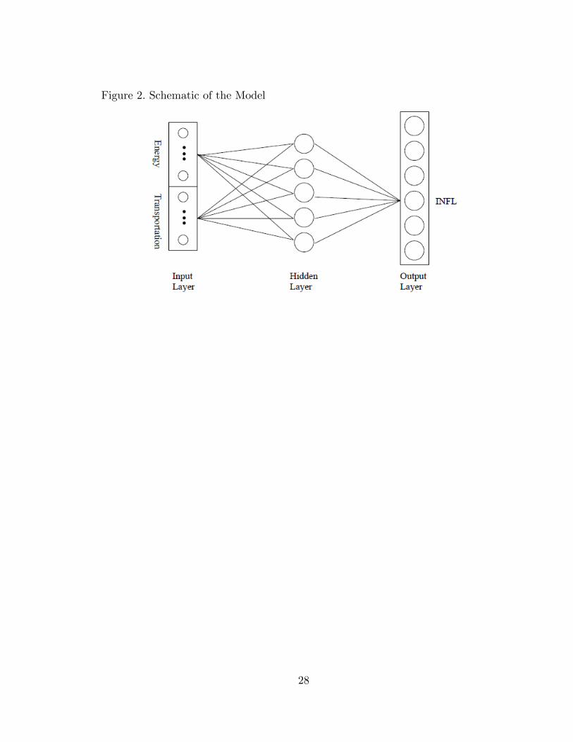
A representative drawing of the selected network architecture is shown in Figure

2. Table 5 summarizes the final accepted model. Column 1 displays the label (number)

assigned to each output node; column 2 displays the associated numerical range.

Column 3 displays the number of extracted rules for each output node. Output node 4

has the largest number of rules (6 rules), while output node 3 has the smallest (3 rules).

Columns 4 and 5 display the numbers of data points within each output range in the

estimation (that is, training) and test datasets, respectively.

Columns 6 and 7 summarize the model’s accuracy during the training

(estimation) and test exercises. In column 6, for example, node 6 was chosen correctly in

240 months and incorrectly in 2 months. Output node 4, with the largest number of

observations, was chosen incorrectly in 60 months, one-fourth of the time. Column 7

displays the same information for the test (holdout) dataset. Choice accuracy is

disappointing for output nodes 3 and 4, that is, headline trend inflation between 2

percent and 3 percent, and between 3 percent and 5 percent.

Analysis of the Extracted Rules

The use of rules to extract and summarize information in neural network models

has a long history. We rely on a decompositional approach to rule extraction, described

in Schmidt (2002) and Schmidt and Chen (2002).15 The 26 extracted rules are displayed

in Table 6.

The rule extraction algorithm works recursively as follows: For each output node,

the algorithm identifies those nodes within the (single) hidden layer that feed the

15 Rule extraction discussions have their own hierarchy. The upper-most categories are “symbolic” and

“connectionist.” The latter contains two sub-categories: pedagogical and decompositional.

Decompositional methods trace the connection of each output node to each hidden node (intermediate

transfer function) and, in turn, each hidden node to the input nodes. At a somewhat lower rank is

“pedagogical extraction” which treats the network as a black box and extracts rules via simultation.

Andrews et al (1995) and Tickle et al (1998), respectively, survey rule extraction algorithms for

feedforward and recursive networks.

16

specific output node; next, the algorithm identifies the input nodes that feed each of

those hidden-layer output nodes, etc. In this manner, the algorithm iteratively

constructs a mapping from the input nodes to the output nodes. For example, the set of

rules extracted for output node 5 exhaustively describe those combinations of values of

the model’s inputs (that is, the set of input nodes) that suggest a trend rate of headline

inflation in the range 5%-9%. There are six nodes in the output layer. The mapping

from a given vector of input values to an output node is one-to-one and onto, that is,

the rule extraction algorithm ensures that the set of input ranges in each rule selects

only a single output node. Extracted rules must replicate the behavior of the model: in

response to a given set of input values, the extracted rules and the model both must

select the same output node.

The output rules are straightforward to interpret as if-then-else constructions.

Rules 1-4, for example, map to output node 1: inflation less than or equal to 1-1/4

percent per annum. Rules 5-8, for example, map to output node 2: inflation between

1.25 percent and 2 percent. Consider node 1 in Table 6. Rule 1 says “if A is true, then

output node 1.” Similarly, rule 3: “if at least one of {C, D, I, K, L} and M are true,

then output node 1” and rule 7: “if E is true and at least 1 of {M, N,…,V, X ,Z} is true,

then output node 2.”16

The extracted rules for the 6 output nodes differ relatively little in complexity.

Note that node 3, corresponding to headline inflation between 2 and 3 percent, has the

smallest number of rules (3), rules 9, 10 and 11. These rules, as a group, display the

weakest dependence of headline inflation on movements in energy and transport prices.

This is completely reasonable because observations during this period comprise much of

the “Great Moderation.” In contrast is output node 6, with a monthly headline CPI

inflation rate exceeding 9 percent. Inflation at that rapid a pace was observed only in

one epoch: May 1979 to September 1981, when inflation was consistently greater than a

9 percent annual rate; subsequently, headline inflation has never again revisited rates

that high. Energy prices also increased at an unusually rapid pace: 20 percent per

annum in May 1979, peaking at a 47 percent pace in May 1980, and continuing at more

than a 10 percent pace through December 1981. For node 6, it would be 20 years until

16 The “MofN” interpretation was introduced by Towell and Shavlik (1993).

17

energy price inflation once again reached a 20 percent rate in March and June 2000—

but then headline inflation was at a 3.7 percent pace. Three of the five rules focus on

rapid energy price inflation; one rule includes 16 of the 17 bins for energy price inflation

(!), and one rule excludes energy entirely while including only very large increases in

transport costs. Considering the unusual type of shocks that generate such inflation, the

rules do a reasonable job of capturing the functional linkages.

Conclusions & Future Work

We have illustrated methods to open the black box that surrounds connectionist

models (statistically oriented neural networks), and have illustrated them with an

application to the inflation pass-through problem. We find rules in line with our priori

expectations, based on extant empirical results in the economics literature.

Our results suggest that, from a policy perspective, there is almost no pass

through from energy prices into trend headline inflation: although our estimated

ANN/rule extraction methods suggest that energy should be included in a number of

rules, the rules have a wide range of values. This is consistent with the economics liter-

ature: energy fluctuates so wildly that it is difficult to infer much from the fluctuations.

The U.S. Federal Reserve’s Federal Open Market Committee has adopted the

core (excluding food and energy prices) chain price index for personal consumption

expenditures ("core PCE") as its policy objective. Both the rules reported here (and

additional experiments comparing the contents of the rules to the binning of

transportation and energy inputs, not included in this paper) have wide variability. In

part, this to be expected because the inflation series are highly volatile.

Our study suggests a number of topics for future research. One is to determine

exactly how to use these rules as a means of applying suitable weights to the

components of personal consumption expenditure so as to take account of the volatility

of food and energy prices in monetary policymaking. Food and energy prices are clearly

important components of households’ everyday budgeting decisions. An additional topic

for future research is to test these rules in an out-of-sample forecasting framework so as

to gain further insights into their validity. Finally, comparative analyses using discrete

multivariate statistics or, alternatively, embedding such rules into a DSGE macro model

likely would yield new insights.

18

References

Andrews, R., J. Diederich, and A. Tickle (1995). Survey and Critique of

Techniques for Extracting Rules from Trained Artificial Neural Networks. Knowledge-

Based Systems, 8(6), 373-389.

Asadi, R., N. Mustapha, N. Sulaiman, N. Shiri (2009). New Supervised Multi

Layer Feed Forward Neural Network Model to Accelerate Classification with High

Accuracy. European Journal of Scientific Research, 33(1), 163-178.

Baesens, B., R. Setiono, C. Mues, and J. Vanthienen (2003). Using Neural

Network Rule Extraction and Decision Tables for Credit-Risk Evaluation. Management

Science, 49(3), 312-329.

Barsky, R.B. and L. Kilian (2001). Do We Really Know That Oil Caused the

Great Stagflation? A Monetary Alternative. In Ben S. Bernanke and Kenneth Rogoff,

eds., NBER Macroeconomics Annual 2001, 16, 137-183.

Bernanke, B. S., M. Gertler, and M. Watson (1997). Systematic Monetary Policy

and the Effects of Oil Price Shocks. Brookings Papers on Economic Activity, 1, 91-142.

Binner, J. M., P. Tino, J. Tepper, R. Anderson, B. Jones and G. Kendall (2010).

Does Money Matter in Inflation Forecasting? Physica A: Statistical Mechanics and its

Applications, 389 (21) 4793-4808.

Bishop, Christopher M. (1995). Neural Networks for Pattern Recognition. Oxford

University Press.

Blanchard, O. and J. Gali (2007). The Macroeconomic Effects of Oil Price

Shocks: Why Are the 2000s So Different from the 1970s? In J. Gali and M. Gertler, eds.,

International Dimensions of Monetary Policy, pp. 373-421. University of Chicago Press

for the NBER (Published in 2010).

Blanchard, O. and M. Riggi (2009). Why Are the 2000s So Different from the

1970s? A Structural Interpretation of Changes in the Macroeconomic Effects of Oil

Prices. NBER working paper 15467.

Blynski, Lev, and Alex Faseruk (2006). Comparison of the Effectiveness of

Option Price Forecasting: Black-Sholes vs. Simple and Hybrid Neural Networks. Journal

of Financial Management and Analysis, 19(2), 46-58.

19

Cecchetti, S. G., P. Hooper, B. C. Kasman, K. L. Schoenholtz, and M. W.

Watson (2007). Understanding the Evolving Inflation Process. US Monetary Policy

Forum working paper.

Chen, Shiu Sheng (2009). Oil Price Pass Through into Inflation. Energy

Economics, 31(1), 126-133.

Chen, Yu-Chin, K.S. Rogoff, and B. Rossi. (2010) Can Exchange Rates Forecast

Commodity Prices? Quarterly Journal of Economics, 125(3), 1145-1194.

Cheng, Bing and D. M. Titterington (1994). Neural Networks: A Review from a

Statistical Perspective. Statistical Science, 9(1) 2-30.

Clark, T. E. and S. J. Terry (2010). Time Variation in the Inflation Passthrough

of Energy Prices. Journal of Money, Credit and Banking, 42(7), 1419-1433.

De Gregorio, O., J. Landerretche, and C. Neilson (2007). Another Pass-Through

Bites the Dust? Oil Prices and Inflation. Central Bank of Chile Working Paper 417.

Faraway, Julian and C. Chatfield (1998). Time Series Forecasting with Neural

Networks: A Comparative Study using Airline Data. Applied Statistics, 47(2), 231-250.

Feldman, J. A. and D. H. Ballard (1982). Connectionist Models and Their

Properties. Cognitive Science, 6, 205-254.

Francis, N. and M. Owyang (2005). Monetary Policy in a Markov-Switching

Vector Error-Correction Model: Implications for the Cost of Disinflation and the Price

Puzzle. Journal of Business and Economic Statistics, 23(3), 305-313.

Gagnon, J. and J. Ihrig (2004). Monetary Policy and Exchange Rate Pass-

Through. International Journal of Finance and Economics, 9(4), 315-338.

Gallant, Stephan (1988). Connectionist Expert Systems. Communications of the

ACM, 31(2) 152-169.

Gallant, Stephan (1993). Neural Network Learning and Expert Systems.

Cambridge: The MIT Press.

Haider, A. and M. N. Hanif (2009). Inflation Forecasting in Pakistan Using

Artificial Neural Networks. Pakistan Economic and Social Review, 47(1), 123-138.

Hamilton, James D. (2003). What Is an Oil Shock? Journal of Econometrics,

113(2), 363-398.

20

Hamilton, James D. (2009). Causes and Consequences of the Oil Shock of 2007-

2008. Brookings Papers on Economic Activity, Spring 2009, 215-259.

Hamilton, James D. and A.M. Herrera (2004). Oil Shocks and Aggregate

Macroeconomic Behavior: The Role of Monetary Policy. Journal of Money, Credit and

Banking, 36(2), 265-286.

Hooker, Mark A. (1996). What Happened to the Oil Price-Macroeconomy

Relationship? Journal of Monetary Economics, 38(2), 195-213.

Hooker, Mark A. (2002). Are Oil Shocks Inflationary? Asymmetric and Nonlinear

Specifcations versus Changes in Regime. Journal of Money, Credit and Banking, 34(2),

540-561.

Hornick, K., L. Stinchcombe and H. White (1989). Multilayer Feedforward

Networks Are Universal Approximators. Neural Networks, 2(5), 359-366.

Hornick, K., L. Stinchcombe and H. White (1990). Universal Approximation of

an Unknown Mapping and Its Derivatives Using Multilayer Feedforward Networks.

Neural Networks, 3(5), 551-560.

Judd, Kenneth (1998). Numerical Methods in Economics. Cambridge: MIT Press.

Kilian, Lutz (2008). The Economic Effects of Energy Price Shocks. Journal of

Economic Literature, 46(4), 871-909.

Kiani, Khurshid M. and Terry L. Kastens (2008). Testing Forecast Accuracy of

Foreign Exchange Rates: Predictions from Feed Forward and Various Recurrent Neural

Network Architectures. Computational Economics, 32(4), 383-406.

Kuan, Chung-Ming and H. White (1994). Artificial Neural Networks: An

Econometric Perspective. Econometric Reviews, 13(1), 1-91.

Lim, G.C. and Paul McNelis (2008). Computational Macroeconomics for the

Open Economy. Cambridge: MIT Press.

McNelis, Paul (2005). Neural Networks in Finance. Elsevier Academic Press.

Medler, David A. (1998). A Brief History of Connectionism. Neural Computing

Surveys, 1(2), 61-101.

Mishkin, F. and K. Schmidt-Hebbel (2001). One Decade of Inflation Targeting in

the World: What Do We Know and What Do We Need to Know? NBER Working

Paper 8397.

21

Mishkin, F. and K. Schmidt-Hebbel (2007). Does Inflation Targeting Make a

Difference? NBER Working Paper 12876.

Nakamura, Emi (2005). Inflation Forecasting Using a Neural Network.

Economics Letters, 86(3), 373-378.

Nordhaus, William D. (2007). Who’s Afraid of a Big Bad Oil Shock? Brookings

Papers on Economic Activity, 2: 219-240.

Owyang, M. and G. Ramey (2004). Regime Switching and Monetary Policy

Measurement. Journal of Monetary Economics, 51(8), 1577-1597.

Orphanides, A. and J. Williams (2002). Robust Monetary Policy Rules with

Unknown Natural Rates. Brookings Papers on Economic Activity, 2, 63-118.

Orphanides, A. and J. Williams (2007). Robust Monetary Policy with Imperfect

Knowledge. Journal of Monetary Economics, 54(5), 1406-1435.

Pradhan, Rudra P. and Ankit Kumar (2008). Forecasting Economic Growth

Using an Artificial Neural Network Model. Journal of Financial Management and

Analysis, 21(1), 24-31.

Rossi, Barbara (2005). Optimal Tests for Nested Model Selection with Underlying

Parameter Instability. Econometric Theory, 21(5), 962-990.

Sarle, Warren S. (1994). Neural Networks and Statistical Models. Proceedings of

the Nineteenth Annual SAS Users Group International Conference.

Schmidt, Vincent A. (2002). An Aggregate Connectionist Approach for

Discovering Association Rules. Ph.D. thesis, Wright State University, Dayton, Ohio.

Schmidt, Vincent A. and C. L. Philip Chen (2002). Using the Aggregate

Feedforward Neural Network for Rule Extraction. International Journal on Fuzzy

Systems, 4(3).

Segal, Paul (2007). Why Do Oil Prices No Longer Shock? Oxford Institute for

Energy Studies Working Paper WPM 35.

Setiono, Rudy and A. Azcarraga (2002). Generating Concise Sets of Linear

Regression Rules from Artificial Neural Networks. International Journal of Artificial

Intelligence Tools, 11(2), 189-202.

Stewart, Kenneth J. and Stephen B. Reed (1999). Consumer Price Index

Research Series Using Current Methods, 1978-98. Monthly Labor Review, 122(6), 29-38.

22

Sulaiman, S., T. Rahman, and I. Musirin (2009). Optimizing One-hidden Layer

Neural Network Design Using Evolutionary Programming. Mimeo. Paper presented at

the 5th International Colloquium on Signal Processing & Its Application.

Swanson, Nonnan R. and Halbert White (1995). A Model Selection Approach to

Assessing the Information in the Term Structure Using Linear Models and Artificial

Neural Networks. Journal of Business and Economic Statistics, 13 (3), 265-275.

Swanson, Norman R. and Halbert White (2007). A Model Selection Approach to

Real-Time Macroeconomic Forecasting Using Linear Models and Artificial Neural

Networks. Review of Economics and Statistics. 79(4) 540-550.

Tickle, A., R. Andrews, M. Golea, and J. Diederich (1998). The Truth Will Come

to Light: Directions and Challenges in Extracting the Knowledge Embedded within

Trained Artificial Neural Networks. IEEE Transactions on Neural Networks, 9(6), 1057-

1068.

Towell, Geoffrey and J. Shavlik (1993). The Extraction of Refined Rules from

Knowledge-Based Neural Networks. Machine Learning, 131, 71-101.

Tsukimoto, H. (2000). Extracting Rules from Trained Neural Networks. IEEE

Transactions on Neural Networks, 11(2), 377-389.

van den Noord, P. and C. Andre (2007). Why Has Core Inflation Remained so

Muted in the Face of the Oil Shock? Organisation for Economic Cooperation and

Development working paper 551.

Weiss, Sholom M. and N. Indurkhya. (1998). Predictive Data Mining: A Practical

Guide. San Francisco: Morgan Kaufmann Publishers Inc.

White, Halbert (1988). Economic Prediction Using Neural Networks: The Case of

IBM Dally Stock Returns, Proceedings of the IEEE International Conference on Neural

Network, 451-458.

White, Halbert (1989). Learning in Artificial Neural Networks: A Statistical

Perspective. Neural Computation, 1(4), 425-464.

White, Halbert (1990). Connectionist Nonparametric Regression: Multilayer

Feedforward Networks Can Learn Arbitrary Mappings, Neural Networks, 3 (5), 535-549

Yildiz, Birol and A. Yezegel (2010). Fundamental Analysis with Artificial Neural

Network. The International Journal of Business and Finance Research, 4(1), 149-158.

23

Zaki, Mohammed J. (1998). Scalable Data Mining for Rules. Technical Report

URCS-TR-702 (Ph.D. thesis), University of Rochester, Rochester, NY.

Energy Transport Housing Food

Panel A:

N=13

N=25

0.00***

0.00***

0.00***

0.00***

0.01***

0.00***

0.22

0.01***

Panel B:

N=13

N=25

0.30

0.29

0.04**

0.07*

0.00***

0.00***

0.05**

0.12

Energy Transport Housing Food

Panel A:

N=13

N=25

0.06

0.31

0.10*

0.37

0.28

0.60

0.02**

0.17

Panel B:

N=13

N=25

0.53

0.35

0.33

0.43

0.00***

0.08*

0.00***

0.15

cp :: Headline CPI

Table 1

Bivariate Granger Causality Tests

cp :: Core CPI (excludes food and energy)

The table shows p-values for the null hypothesis of Granger causality. Asterisks mark significance at the 1%

(***), 5% (**), and 10% (*) levels, suggesting support for Granger causality.

::tz

0 10 0

-values of H : 0 inN N

j t j t j j t jj j

p j cp cp zg a b g+ - -= =

= " D = + D + Då å

0 10 0

-values of H : 0 inN N

j t j t j j t jj j

p j z z cpg a b g+ - -= =

= " D = + D + Då å

::tz

0 10 0

-values of H : 0 inN N

j t j t j j t jj j

p j cp cp zg a b g+ - -= =

= " D = + D + Då å

0 1 ,0 0

-values of H : 0 inN N

j t j t j j t t jj j

p j z z cpg a b g+ - -= =

= " D = + D + Då å

Energy Transport Housing Food

Panel A:

N=13 0.58 0.21 0.53 0.30

N=25 0.77 0.46 0.86 0.49

Panel B:

N=13 0.79 0.26 0.51 0.19

N=25 0.98 0.49 0.85 0.27

Energy Transport Housing Food

Panel A:

N=13 0.22 0.42 0.38 0.53

N=25 0.37 0.50 0.59 0.77

Panel B:

N=13 0.63 0.63 0.73 0.69

N=25 0.46 0.44 0.65 0.61

Table 2

Andrew's (1993) QLR Test for Instabilities

cp :: Headline CPI

cp :: Core CPI (excludes food and energy)

The table reports p-values for Andrew's (1993) "QLR" test of temporal parameter stability. In those sections labled Panel A, headline and

core CPI are the dependent variables and component subindexes are the regressors. In those sections labeled Panel B, the headline and

core CPI series are the regressors. In no case is the null of parameter stability rejected.

( ) ( )0 0, , 0 1 0, ,0 0

-values for : , = , inN N

t j t j t t j t j j t t jj j

p H j z z cpg g g g g b g+ - -= =

" D = + D + Då å

::tz

( ) ( )0 0, , 0 1 0, ,0 0

-values for : , = , inN N

t j t j t t j t j j t t jj j

p H j cp cp zg g g g g b g+ - -= =

" D = + D + Då å

::tz

( ) ( )0 0, , 0 1 0, ,0 0

-values for : , = , inN N

t j t j t t j t j j t t jj j

p H j cp cp zg g g g g b g+ - -= =

" D = + D + Då å

( ) ( )0 0, , 0 1 0, ,0 0

-values for : , = , inN N

t j t j t t j t j j t t jj j

p H j z z cpg g g g g b g+ - -= =

" D = + D + Då å

Energy Transport Housing Food

Panel A:

N=13 0.025** <0.01*** 0.029** >0.10

N=25 0.070* <0.01*** 0.082* 0.036**

Panel B:

N=13 >0.10 0.043** <0.01*** 0.043**

N=25 >0.10 >0.10 0.027** 0.096*

Energy Transport Housing Food

cp :: Headline CPI

cp :: Core CPI (headline CPI excluding food and energy)

Table 3

Granger Causality Tests Robust to Instabilities (Rossi, 2005)

0 , 1 ,0 0

-values for : 0 inN N

j t t j t j j t t jj i

p H j cp cp zg g a b g+ - -= =

= = " D = + D + Då å

0 , 1 ,0 0

-values for : 0 inN N

j t t j t j j t t jj i

p H j z z cpg g a b g+ - -= =

= = " D = + D + Då å

0 , 1 ,0 0

-values for : 0 inN N

j t t j t j j t t jj i

p H j cp cp zg g a b g+ - -= =

= = " D = + D + Då å

0 , 1 ,0 0

-values for : 0 inN N

j t t j t j j t t jj j

p H j z z cpg g a b g+ - -= =

= = " D = + D + Då å

::tz

::tz

Panel A:

N=13 0.051* >0.10 0.050** 0.071*

N=25 >0.10 >0.10 >0.10 >0.10

Panel B:

N=13 >0.10 >0.10 0.042** 0.025**

N=25 >0.10 >0.10 >0.10 >0.10

The table reports p-values for the null hypotheses that each of the four component price indexes does not Granger-cause the headline or core CPI, adjusted for instabilities as in Rossi (2005). Asterisks indicate rejection of the null at the 1% (***), 5% (**), and 10% (*) levels. We test at two lag lengths: the AIC generally suggested 24 lags, the BIC suggested 12. For robustness, we increase each lag by one.

0 , 1 ,0 0

-values for : 0 inN N

j t t j t j j t t jj i

p H j cp cp zg g a b g+ - -= =

= = " D = + D + Då å

0 , 1 ,0 0

-values for : 0 inN N

j t t j t j j t t jj i

p H j z z cpg g a b g+ - -= =

= = " D = + D + Då å

0 , 1 ,0 0

-values for : 0 inN N

j t t j t j j t t jj i

p H j cp cp zg g a b g+ - -= =

= = " D = + D + Då å

0 , 1 ,0 0

-values for : 0 inN N

j t t j t j j t t jj j

p H j z z cpg g a b g+ - -= =

= = " D = + D + Då å

::tz

::tz

24

Table 4. Input and Output Ranges, and Observations per Range (Combined Training

and Test Datasets)

Number of 

Observations

Number of 

Observations

Number of 

Observations

Lower 

Bound

<=

Upper 

Bound

<

Lower 

Bound

<=

Upper 

Bound

<

Lower 

Bound

<=

Upper 

Bound

<

A        ‐Inf ‐0.121254 7 M       ‐Inf ‐0.265215 2 1 ‐inf 0.0125 19

B ‐0.121254 ‐0.101202 2 N ‐0.265215 ‐0.204803 6 2 0.012500 0.020000 48

C ‐0.101202 ‐0.070711 2 O ‐0.204803 ‐0.107416 21 3 0.020000 0.030000 113

D ‐0.070711 ‐0.032497 17 P ‐0.107416 ‐0.022121 38 4 0.030000 0.050000 134

E ‐0.032497 ‐0.011131 25 Q ‐0.022121 0.050777 155 5 0.050000 0.090000 30

F ‐0.011131 0.014684 41 R 0.050777 0.106695 54 6 0.090000 inf 29

G 0.014684 0.074562 217 S 0.106695 0.138965 18

H 0.074562 0.135777 40 T 0.138965 0.163726 22

I 0.135777 0.166635 11 U 0.163726 0.185737 15

J 0.166635 0.192465 6 V 0.185737 0.215139 14

K 0.192465 0.220937 3 W 0.215139 0.253502 11

L 0.220937          Inf 2 X 0.253502 0.282514 1

Y 0.282514 0.321399 4

Z 0.321399 0.371623 6

AA 0.371623 0.409081 2

AB 0.409081 0.447016 2

AC 0.447016          Inf 2

Transportation ranges Energy ranges Output ranges

Input and Output Ranges, and Number of Observations per Range

25

Table 5: Accuracy of the Trained Model

Output "Infation % change" Train Test Net Train Accuracy Net Test Accuracy Node Range (min,max) Rules Targets Targets Correct of 242, % Correct of 131, %

1 < 1.25% 4 10 9 (237) 97.93% (127) 96.95% 2 (1.25%, 2.0%) 4 32 16 (223) 92.15% (116) 88.55% 3 (2.0%, 3.0%) 3 72 41 (174) 71.90% (85) 64.89% 4 (3.0%, 5.0%) 6 90 44 (182) 75.21% (84) 64.12% 5 (5.0%, 9.0%) 4 18 12 (230) 95.04% (117) 89.31% 6 > 9.0% 5 20 9 (240) 99.17% (123) 93.89%

26

Table 6. Graphical Representation of Extracted Rules

Graphical representation of ranges used in output nodes (rules)

1 2 3 4 5 6 7 8 9 10 11 12 13 14 15 16 17 18 19 20 21 22 23 24 25 26

Input

Range

Transportation ranges

A        ‐Inf ‐0.121254 X X

B ‐0.121254 ‐0.101202 X X X

C ‐0.101202 ‐0.070711 X X X X X

D ‐0.070711 ‐0.032497 X X X X X

E ‐0.032497 ‐0.011131 X X X X X

F ‐0.011131 0.014684 X X X X X

G 0.014684 0.074562 X X X X X

H 0.074562 0.135777 X X X X

I 0.135777 0.166635 X X X   X

J 0.166635 0.192465 X X X

K 0.192465 0.220937 X X X

L 0.220937          Inf X X X

Energy ranges

M       ‐Inf ‐0.265215 X X X X X X X X

N ‐0.265215 ‐0.204803 X X X X X X X X

O ‐0.204803 ‐0.107416 X X X X X X X X X

P ‐0.107416 ‐0.022121 X X X X X X X X

Q ‐0.022121 0.050777 X X X X X X X X

R 0.050777 0.106695 X X X X X X X X

S 0.106695 0.138965 X X X X   X X X

T 0.138965 0.163726 X X X X X X X X X X

U 0.163726 0.185737 X X X X X X X X X X

V 0.185737 0.215139 X X X X X X X X X X

W 0.215139 0.253502 X X X X X X X

X 0.253502 0.282514 X X X X X  X X X

Y 0.282514 0.321399 X X X X X X    X

Z 0.321399 0.371623 X X X X X X

AA 0.371623 0.409081 X X X X X X X X

AB 0.409081 0.447016 X X X X X X X X

AC 0.447016          Inf X X X X X X X X

Output Nodes

Rule Number >

Node 3

(2.0... 3.0]

Node 2

(0.0125... 2.0]

Node 1

[‐inf, 0.0125]

Node 6

(9.0... Inf]

Node 5

(5.0... 9.0]

Node 4

(3.0... 5.0]

27

Figure 1

Lower 

Bound

<=

Upper 

Bound

< T1 T2 T3 T4 T5

1 ‐inf 0.0125 0 0 0 0 0

2 0.0125 0.0200 0 0 0 0 1

3 0.0200 0.0300 0 0 0 1 1

4 0.0300 0.0500 0 0 1 1 1

5 0.0500 0.0900 0 1 1 1 1

6 0.0900 inf 1 1 1 1 1

Dec‐78 0.0790 0 1 1 1 1

Jan‐79 0.0816 0 1 1 1 1

Feb‐79 0.0851 0 1 1 1 1

Mar‐79 0.0874 0 1 1 1 1

Apr‐79 0.0886 0 1 1 1 1

May‐79 0.0907 1 1 1 1 1

Jun‐79 0.0908 1 1 1 1 1

Oct‐81 0.0887 0 1 1 1 1

Nov‐81 0.0867 0 1 1 1 1

Dec‐81 0.0831 0 1 1 1 1

Dec‐82 0.0509 0 1 1 1 1

Jan‐83 0.0479 0 0 1 1 1

Feb‐83 0.0449 0 0 1 1 1

Mar‐83 0.0442 0 0 1 1 1

Apr‐83 0.0503 0 1 1 1 1

May‐83 0.0486 0 0 1 1 1

Jun‐83 0.0427 0 0 1 1 1

Jan‐86 0.0381 0 0 1 1 1

Feb‐86 0.0306 0 0 1 1 1

Mar‐86 0.0213 0 0 0 1 1

Apr‐86 0.0146 0 0 0 0 1

Output ranges Thermometer Variables

Selected Dates

Example of Thermometer Encoding, Based on Headline Inflation Rate

28

Figure 2. Schematic of the Model