Theor EcolDOI 10.1007/s12080-008-0017-1

ORIGINAL PAPER

Connecting host physiology to host resistancein the conifer-bark beetle system

William A. Nelson · Mark A. Lewis

Received: 12 May 2007 / Accepted: 20 February 2008© Springer Science + Business Media B.V. 2008

Abstract Host defenses can generate Allee effects inpathogen populations when the ability of the pathogento overwhelm the defense system is density-dependent.The host–pathogen interaction between conifer hostsand bark beetles is a good example of such a system.If the density of attacking beetles on a host tree islower than a critical threshold, the host repels theattack and kills the beetles. If attack densities areabove the threshold, then beetles kill the host treeand successfully reproduce. While the threshold hasbeen found to correlate strongly with host growth, anexplicit link between host physiology and host defensehas not been established. In this article, we revisitpublished models for conifer-bark beetle interactionsand demonstrate that the stability of the steady statesis not consistent with empirical observations. Based onthese results, we develop a new model that explicitlydescribes host damage caused by the pathogen and usethe physiological characteristics of the host to relatehost growth to defense. We parameterize the model for

W. A. Nelson (B)Department of Biological Sciences, University of Alberta,Edmonton, Alberta, Canadae-mail: nelsonw@queensu.ca

M. A. LewisDepartment of Mathematical and Statistical Sciences,University of Alberta, Edmonton, Alberta, Canadae-mail: mlewis@math.ualberta.ca

Present Address:W. A. NelsonDepartment of Biology, Queen’s University,Kingston, Ontario, Canada

mountain pine beetles and compare model predictionswith independent data on the threshold for successfulattack. The agreement between model prediction andthe observed threshold suggests the new model is aneffective description of the host–pathogen interaction.As a result of the link between the host–pathogen in-teraction and the emergent Allee effect, our model canbe used to better understand how the characteristics ofdifferent bark beetle and host species influence host–pathogen dynamics in this system.

Keywords Host–pathogen models · Attack threshold ·Allee effect · Bark beetles · Resin defenses ·Mountain pine beetles · Carbon budget model

Introduction

Hosts can generate Allee effects (Allee 1931) in apathogen population when host defense depends onpathogen densities (Courchamp et al. 1999; Ogden et al.2002; Uma Devi and Uma Maheswara Rao 2006). Barkbeetles are a classic example of a pathogen that suffersan Allee effect from host resistance (Berryman 1979).Bark beetles are a common and destructive pathogen ofpine forests (Logan and Powell 2001) that must kill hosttissue to ensure successful survival and reproduction(Christiansen et al. 1987; Raffa et al. 2005). As a resultof host defenses, many individual beetles are requiredto successfully overwhelm and kill a single host tree(e.g., Christiansen et al. 1987; Fig. 1). Most species ofbark beetles have evolved a pheromone communica-tion system that helps aggregate the beetle popula-tion during flight (Raffa 2001). If insufficient beetlesare available to attack a host, then host defenses kill

Theor Ecol

Host Vigor (grams M-2

yr-1

)

0 50 100

Beetle A

ttacks

(M-2

)

0

50

100

150

200

Fig. 1 Empirical threshold for successful attack of mountain pinebeetles as a function of host vigor (data from Waring and Pitman1985). Vigor is defined as the mass of wood added to a host treeper year divided by the leaf area. Each symbol represents anindividual tree. Solid circles indicate trees killed by beetles, opencircles are living trees that resisted beetle attack, and gray circlesare living trees where a portion of the bark area was killed bybeetles. The gray line is the empirically estimated threshold forhost mortality

the attacking beetles. If the attack density is above acritical threshold, then attacking beetles kill the hosttree and successfully reproduce. Because beetle sur-vival is tightly coupled to host defense, the thresholdfor successful attack on an individual tree produces apopulation-level Allee effect in bark beetles (Berrymanand Stenseth 1989). Owing to the close host–pathogeninteraction between conifer trees and bark beetles, aswell as the economic impact of this pest species, a gooddeal of empirical and theoretical research has beencarried out.

A number of models have been developed to de-scribe the host–pathogen interaction in bark beetles(Berryman et al. 1989; Stenseth 1989; Powell et al.1996). However, these models blend two distinctprocesses: the host–pathogen interaction within thetree and the immigration of new beetles to the host tree.Biologically, these processes can be separated becausethey occur over different time scales. Beetle immigra-tion is mediated by aggregation pheromones that aregenerated by beetles in the process of attacking a hosttree. These pheromones can attract additional beetlesto the host tree from those flying in the local vicinity(Raffa 2001). Such pheromone-mediated immigration

occurs at the start of an attack and lasts less than aweek (e.g., Raffa and Berryman 1983). In contrast,host death from high attack densities occurs between4 and 6 weeks after the attack has started (Kirisits andOffenthaler 2002). The difference is time scales suggestthat the host–pathogen interaction operates at a slowerrate than beetle migration. This is also supported byempirical observations of the attack threshold (e.g.,Fig. 1), that are well described by the beetle attackdensity after all migration has occurred. Thus, from theperspective of the host–pathogen interaction, the effectof pheromone-mediated immigration can be thought ofas influencing initial attack density.

In this article, we analyze existing bark beetle modelsin the absence of recruitment from flying beetles tostudy the core host–pathogen interaction. Our resultsreveal that these modified models predict unrealisticsteady state characteristics, suggesting that current de-scriptions of the beetle–host interaction need furtherdevelopment. Based on these results, we develop anew model of the beetle–host interaction that explicitlydescribes host damage and demonstrate that it hasbiologically realistic steady state characteristics. Usingwhat is known about tree physiology, we then derive alink between host growth and resin production underthe assumption that growth in carbohydrate is limited.In doing so, we provide the first model to integratephysiologically based host resin defense with process-based attacking beetle dynamics. We parameterize themodel for mountain pine beetles using literature dataand compare model predictions against independentempirical data on the attack threshold in mountain pinebeetles. The success of our new model at predicting theempirical threshold suggests the new model reflects amore accurate description of the beetle–host interac-tion that can be used to understand how the character-istics of the host–pathogen interaction influence beetlepopulation dynamics.

Reanalysis of published models

To begin, we reanalyze previous models of the host–pathogen interaction in the absence of recruitmentfrom flying beetles.

Berryman et al. (1989) and Stenseth (1989)

One of the earlier models of the host–pathogen inter-action was developed by Berryman et al. (1989). Asimilar model is presented in Stenseth (1989), whichis analyzed in Appendix A. Berryman et al. (1989)

Theor Ecol

developed a model of the beetle–host interaction thatexplicitly describes the processes of beetle attack, hostresin defense, and immigration from flying beetles. Themodel is given by

dAdt

=beetle recruitment

︷ ︸︸ ︷

b1(b2 − b3 R)AR −mortality︷ ︸︸ ︷

b4 AR (1)

dRdt

=resin production︷ ︸︸ ︷

b5(1 − b6 A)−resin loss︷︸︸︷

b7 R (2)

where A(t) is the density of attacking beetles per treeand R(t) is the volume of resin per beetle gallery. Thefirst term of Eq. 1 is recruitment from flying beetlesdue to host attractiveness, where b1 is the size of thelocal flying beetle population and parameters b2 and b3

reflect the attractiveness/repellency of the as a functionof resin volume. The second term is beetle mortality,where b4 is the rate at which per capita mortality in-creases with resin volume. Equation 2 describes resindynamics in the host, where b5 is the maximum rate ofresin production of the host, b6 is the decrease in resinproduction caused by attacking beetles, and b7 is theresin loss rate through the attack holes.

Because we are interested in studying beetle–hostdynamics in the absence of immigration from flyingbeetles, we remove the recruitment term from Eq. 1.Introducing the following dimensionless variables

A = Ab6, R = Rb7

b5, t = tb7

and the dimensionless parameter

α = b4b5

b72

we can write a dimensionless version of the modifiedmodel as (after dropping the tildes)

dAdt

= −αAR (3)

dRdt

= 1 − A − R (4)

The model given by Eqs. 3 and 4 has two steady states.The first is (A∗, R∗) = (0, 1), which is a steady statewhere the tree is alive and all attacking beetles aredead. The second is (A∗, R∗) = (1, 0), which is a steady

state where the beetles have successfully killed the hosttree. The Jacobian of Eqs. 3 and 4 is given by

J(A∗,R∗) =(−αR∗ −αA∗

−1 −1

)

(5)

At the steady state (A∗, R∗) = (0, 1), both eigenvaluesare negative, which means that the tree-alive steadystate is stable. At the steady state (A∗, R∗) = (1, 0), oneeigenvalue is negative and one is positive. Thus, thetree-dead steady state is an unstable saddle. An unsta-ble tree-dead steady state means that beetles do notkill host trees in the absence of continual recruitmentfrom flying beetles, regardless of the initial density ofattacking beetles. However, because continual beetleimmigration is not a requirement for host death innature, one or more of the key biological interactionsis missing from the model of Berryman et al. (1989).Figure 2 shows the isoclines, steady states, and examplephase plane trajectories.

Powell et al. (1996)

Powell et al. (1996) developed a mechanistic model ofbeetle dispersal and attack that describes the dynam-ics of flying beetles, attacking beetles, host resin, andpheromones. The model is spatially explicit, and it isdescribed by a set of six partial differential equations.To extract the beetle–host interaction in the absence of

Fig. 2 Example trajectories for the model of Berryman et al.(1989) in the absence of recruitment from flying beetles. Dashedlines show the attacking beetle and resin isoclines. Gray circlesdepict the steady states; the solid circle is a stable steady stateand the open circle is unstable. The black lines are exampletrajectories for α = 0.5, and solid black circles denote initialconditions

Theor Ecol

flying beetle recruitment, we assume that the density ofattacking beetles changes only as a result of mortalityfrom host defenses. With this assumption, the beetle–host interaction is described by the following set ofequations

dAdt

= −p1 AR (6)

dHdt

= −p5 HR (7)

dRdt

= p2(p3 − R)R − p4 HR (8)

where A(t) is the density of beetles attacking a host,H(t) is the number of holes in a host produced by theattacking beetles, and R(t) is the abundance of resin ina host. From Eq. 6, the attacking beetle density declinesfrom resin-caused mortality, where p1 is the rate atwhich the per capita beetle mortality rate increases withresin. Resin is lost through the holes bored by attackingbeetles, where p5 is the rate at which the hole-fillingrate increases with resin abundance. If we assume thateach attacking beetle bores a single hole, then H(0) =Ho = Ao. Resin production is described by the firstterm of Eq. 8, where p2 is the maximum per capitarate of resin renewal and p3 is the maximum amount ofresin in the absence of attacking beetles. Powell et al.(1996) consider that host vigor is described by p3; themaximum capacity of the host to hold resin. However,as we show below, p3 drops out in the process ofnondimensionalization. As an alternative, we considerp2 a measure of host vigor because it reflects the abilityof the host to produce resin and does not drop out inthe process of nondimensionalization.

Because the resin dynamics given by Eq. 8 are in-dependent of attacking beetle density, the model dy-namics can be understood by studying the coupledEqs. 7 and 8. We introduce the following dimensionlessvariables

H = Hp3

p4

p5, R = R

1

p3, t = tp3 p5

and dimensionless parameter

β = p2

p5

to write the modified dimensionless model as (afterdropping the tildes)

dHdt

= −HR (9)

dRdt

= β(1 − R)R − HR (10)

The model given by Eqs. 9–10 has two steady states.The first is (H∗, R∗) = (0, 1), which is a steady statewhere the tree is alive and the attacking beetles aredead. The second steady state is (H∗, R∗) = (H, 0),where H can be any value between zero and the initialnumber of holes (i.e., 0 ≤ H ≤ Ho). More precisely,H is an infinite set of steady states that all satisfyEqs. 9 and 10 at equilibrium (Fig. 3). Biologically, theinfinite set of steady states reflects a situation wherethe host has been killed and a variable number ofholes and attacking beetles remain alive. The numberof holes remaining depends on the outcome of thedynamical process and, thus, on the initial numberattacking beetles and the parameter β. For brevity,we refer to the infinite set of steady states simply asa steady state in the text below. The stability analysisis presented in Appendix B. Similar to the modifiedBerryman et al. (1989) model, the tree-alive steadystate given by (H∗, R∗) = (0, 1) is stable. The tree-deadsteady state is also stable if H > β, but it is unstableif H < β. As a result, the host–pathogen interactionat the core of the Powell et al. (1996) model does nothave the characteristics observed in nature. Figure 3shows the isoclines, steady states, and example phaseplane trajectories for the model given by Eqs. 10 and 9.

Fig. 3 Phase plane diagram for the beetle–host model of Powellet al. (1996) in the absence of recruitment from flying beetles.Dashed lines show the attacking hole and resin isoclines. Thegray symbols are steady states; the circle represents a point steadystate and the thick line represents an infinite set of steady states.Solid symbols are stable steady states and open symbols areunstable. The transition between unstable and stable regions ofthe dead host steady state (thick gray line) occurs when H = β.The black lines show example trajectories for β = 0.5, and theseparatrix is shown in bold

Theor Ecol

A new model for the host–pathogen interaction

Empirical data on the threshold for bark beetle survival(e.g., Mulock and Christiansen 1986; Fig. 1) suggestthat the process of aggregation, whereby flying beetlesare attracted to new hosts by the pheromones emittedfrom attacking beetles, does not have a direct influenceon the beetle–host interaction beyond determining theinitial attack density. Our reanalysis of the publishedmodels by Berryman et al. (1989), Stenseth (1989), andPowell et al. (1996) reveals that, when flying beetlerecruitment is removed from the beetle–host interac-tion, the dead-host steady state becomes unstable forsome parameter values. Biologically, this implies thattrees cannot be killed without continuous beetle im-migration, which is not what occurs in nature. In thenext section, we develop a new model of the beetle–host interaction that resolves this problem by explicitlyincluding host damage caused by attacking beetles. Asabove, we assume that the process of beetle aggregationcan be subsumed into the initial attack density (seeAppendix E for validation of this assumption). Webegin by developing a general model that describes thebeetle–host interaction with undefined functions andstudy the steady states. In the next section, we considera linear form of the general model and study the char-acteristics and stability of the emergent threshold forbark beetle survival.

General model

Resin production by a host tree is considered theprimary mechanism of defense against bark beetles(Christiansen et al. 1987; Franceschi et al. 2005). Priorto an attack, the phloem tissue contains some amountsof preformed resin, which is referred to as the con-stitutive defense. At the start of an attack, resin isproduced in the phloem tissue around the attack site(referred to as the induced defense) (Christiansen et al.1987; Lewinsohn et al. 1991; Raffa and Smalley 1995).Induced resin is derived from carbohydrates in thephloem tissue surrounding the attack site (Trapp andCroteau 2001). Because carbohydrates are producedby photosynthesis in the leaves, both the productionand the transport of carbohydrates to the attack sitebecome determinants of resin production (Christiansenet al. 1987). This process of induced defense is well sup-ported by empirical evidence, which demonstrates thatinterfering with the host’s ability to supply or transportcarbohydrates has a large influence on resin productionand the ability of the host to defend against bark beetleattack (Lombardero et al. 2000; Wallin and Raffa 2001;

Miller and Berryman 1986). Phloem tissue is composedof densely packed sieve tubes and is the main transportpath for carbohydrates from the leaves to the attacksites. As a result, attacking beetles can interfere withhost defense by either diluting resin production amongnumerous attack sites or by damaging phloem tissueand thereby reducing carbohydrate transport.

These empirical observations suggest that a dynamicmodel of both constitutive and induced defenses re-quires three components: resin volume, attacking bee-tles, and the undamaged phloem tissue necessary forcarbohydrate transport. Similar to the previously pub-lished models, the model proposed here includes theability of the host to produce resin. The key modifi-cation is an explicit representation of damage to thecarbohydrate transport pathway. In general, such amodel can be described by

dAdt

= −Ah(R) (11)

dSdt

= −Sk(A) (12)

dRdt

= Sf (R) − Rg(A) (13)

where A(t) is the number of attacking beetles stillalive in the tree, S(t) is the number of undamagedsieve tubes in the tree, and R(t) is the resin volume ofthe host tree. The function f (R) describes the rate ofresin production per undamaged sieve tube. As such,it is a phenomenalistic representation of carbohydrateproduction, carbohydrate transport, and conversion ofcarbohydrates to resin.

Carbohydrate transport through sieve tubes isgoverned by osmoregulatory flow (Thompson andHolbrook 2003), which suggest that resin productionshould be at a maximum fm when no resin is present(i.e., f (0) = fm) and decrease with increasing resinvolume (i.e., f ′(R) < 0) until it reaches zero at the max-imum resin capacity Rm (i.e., f (Rm) = 0). The functiong(A) describes resin metabolism by beetles, which weassume is a monotonically increasing function of beetledensity (i.e., g′(A) > 0) that goes to zero when there areno attacking beetles still alive (i.e., g(0) = 0). Attackingbeetle dynamics are given by Eq. 11, where the functionh(R) describes beetle mortality due to resin. Empiricaldata suggest that greater amounts of resin cause greatermortality rates in beetles (e.g., Raffa and Smalley 1995),so we constrain the function h(R) to be a monotonicallyincreasing function of resin abundance (i.e., h′(R) > 0)

Theor Ecol

with the constraint that h(0) = 0. We model the sievetube damage caused by attacking beetles (including anyassociated fungus) as a per capita sieve tube loss ratek(A) that increases monotonically with the number ofattacking beetles still alive (i.e., k′(A) > 0), and withthe constraint that k(0) = 0. The host is dead when allthe sieve tubes are damaged (i.e., S = 0). The defini-tions and constraints for the general model are summa-rized in Table 1.

Steady state solutions

The constraints described above are sufficient to de-termine steady states of the general model, withoutthe need to specify functions. The model given byEqs. 11–13 has three steady states: (A∗, S∗, R∗) =(A, 0, 0), (0, 0, R), and (0, S, Rm). A is the final numberof attacking beetles and can be any value between zeroand the initial number of attacks (i.e., 0 ≤ A ≤ Ao).Similarly, R is the final resin volume between zero andthe initial resin volume (i.e., 0 ≤ R ≤ Ro), and S is thefinal number of sieve tubes between zero and the initialnumber (i.e., 0 ≤ S ≤ So).

Biologically, the steady states are qualitatively sim-ilar to those predicted by the previously publishedmodels. At the steady state (A∗, S∗, R∗) = (0, S, Rm),all attacking beetles are dead and the host tree is atmaximum resin capacity with some amount of undam-aged sieve tubes remaining. The proportion of dam-aged sieve tubes indicates the amount of permanentdamage caused by the unsuccessful beetle attacks (i.e.,1 − S/So). At the steady state (A∗, S∗, R∗) = (A, 0, 0),the attacking beetles have damaged all sieve tubesand killed the host tree. The last steady state is givenby (A∗, S∗, R∗) = (0, 0, R), which reflects a situationwhere the attacking beetles damaged all of the hostsieve tubes and the remaining resin was sufficient to killthe beetles, with the end result that both the beetles andhost are dead.

Linear model

We consider a model with linear functions. Let f (R) =fo

(

1 − RRm

)

, g(A) = go A, h(R) = ho R, and k(A) =ko A. Parameter fo is the maximum resin productionrate per sieve tube, Rm is the maximum resin volume,go is the rate at which the resin loss rate changes withthe number of attacking beetles, ho is the rate at whichbeetle mortality changes with resin volume, and ko

is the rate at which the sieve tube loss rate changeswith the number of attacking beetles. Introducing thefollowing dimensionless variables

A = Ago

ho Rm, S = S

So, R = R

Rm, t = tho Rm (14)

and dimensionless parameters

γ = So fo

R2mho

, ζ = ko

go(15)

allows us to write the following dimensionless model(after dropping the tildes)

dAdt

= −AR (16)

dSdt

= −ζ AS (17)

dRdt

= γ S(1 − R) − AR (18)

The nondimensional steady states are (A, 0, 0),(0, 0, R), and (0, S, 1), where 0 ≤ A < ∞, 0 ≤ R ≤ 1,and 0 ≤ S ≤ 1. The initial conditions are (Ao, 1, Ro),where 0 ≤ Ro ≤ 1 and 0 ≤ Ao ≤ ∞. The two steadystates of biological interest are the live beetle – deadhost state (A∗, S∗, R∗) = (A, 0, 0) – and the deadbeetle—live host state (A∗, S∗, R∗) = (0, S, 1). Both ofthese steady states are stable for γ and A slightlygreater than zero (Appendix C). Thus, and in con-trast to our reanalysis of published models, the host–

Table 1 Symbol definitionsand constraints for thegeneral model

Symbol Definition Constraints

A Number of attacking beetles per tree A ≥ 0S Number of sieve tubes per tree S ≥ 0R Resin volume per tree R ≥ 0t Time index –Rm Maximum resin volume per tree Rm ≥ 0fm Maximum resin production rate fm ≥ 0f (R) Per capita resin production function f (0) = fm, f (Rm) = 0, f ′(R) < 0g(A) Per capita resin loss rate g(0) = 0, g′(A) > 0h(R) Per capita beetle mortality function h(0) = 0, h′(R) > 0k(A) Per capita sieve tube damage rate k(0) = 0, k′(A) > 0

Theor Ecol

pathogen model developed here has steady states thatare consistent with empirical observations.

Dynamics of the linear model given by Eqs. 16–18are governed by two parameters γ and ζ . Biologically,γ is the ratio of maximum resin production to maxi-mum beetle mortality and ζ is the ratio of the phloemdamage rate to the resin removal rate. To understandthe magnitude of initial attack density required to killa host tree, and how this is influenced by the parame-ters, we study the threshold behavior using numericalsimulations of the model trajectories. Figure 4 showsexample trajectories of the linear model. At high initial

Fig. 4 Example trajectories for the linear model given byEqs. 16–18. Each line shows a trajectory starting from differentinitial beetle densities Ao. The dynamics are shown for γ = 8and ζ = 1, and arrows show the direction of time. a Trajectoriesin the full 3D phase space. Circles are initial conditions, and thebold lines are steady states. Solid lines are stable steady states,and the dashed line is the unstable steady state. b Projectionof the 3D trajectories onto the R-A plane. The gray line showsthe trajectory emerging from the critical initial beetle abundanceAo

c, above which beetle attacks kill the host tree and belowwhich the host kills the attacking beetles

Fig. 5 Asymptotic host responses. Proportion of host damagedafter the attack process ((1 − S∗); black line) and the minimumresin abundance (gray line) for parameter values shown in Fig. 4.The critical attack density (Ac

o) is shown with the dashed line

beetle abundance, beetles quickly kill the host tree.As the number of initial beetles decreases, the host isstill killed but the number of beetles remaining alsodecreases. Below the critical initial beetle abundanceAo

c, the host repels the attack and all beetles are killed.Further decreases in the initial beetle abundance havethe effect of reducing the level of damage sustainedby the host before the beetles are killed. The criticalinitial beetle abundance Ao

c is defined as the value ofAo that results in (A∗, S∗, R∗) = (0, 0, 0) and representsthe threshold for beetle survival. Because there is noanalytical solution to Eqs. 16–18, we determined Ao

c

numerically. When host trees survive attacks, the re-sulting damage and resin densities depend on the initialdensity of attacking beetles (Fig. 5). Even if attackdensities are lower than the critical threshold, the hosttree can still suffer substantial damage.

The critical threshold Aoc depends on parameters γ

and ζ . The empirical observations of Fig. 1 indicate thatgreater numbers of beetles are required to kill hostswith higher levels of vigor. For these data, vigor is de-fined as the volume of wood produced per year relativeto the leaf area, which reflects growth efficiency of thehost (Waring et al. 1980). The rationale for studyingthe influence of host vigor on the threshold for success-ful beetle attack is that trees able to produce greateramounts of wood have higher carbohydrate produc-tion and, thus, should also be able to produce greateramounts of resin if attacked. We develop this linkquantitatively in the next section. Qualitatively, how-ever, greater host vigor corresponds to greater resin

Theor Ecol

Fig. 6 Critical threshold of initial attacking beetle abundanceAo

c as a function of host resin production for the linear modelgiven by Eqs. 16–18. Thresholds are shown for ζ = 0.5 (blackline), ζ = 1 (dark gray line), and ζ = 2 (light gray line). Thegray point shows the critical attack density (Ao

c) for the graytrajectory of Fig. 4

production. In the linear model, this is the γ parameter.Figure 6 shows how the critical threshold changes as afunction of γ .

The linear model predicts that the threshold Aoc

should increase with increasing ability of the host toproduce resin. Qualitatively, this agrees well with theempirical data (Fig. 1). In the following section, we linkresin production to host vigor quantitatively and fullyparameterize the model for mountain pine beetles us-ing independent literature data. To assess the relevanceof the mechanisms described by the model, we thencompare the quantitative predictions from the linearmodel with the empirical threshold of Fig. 1.

Parameterization of the linear model

Linking host vigor to resin production

Carbohydrate production for a tree can be describedby loL, where L is the leaf area of the tree and lo isthe per-unit leaf area rate of carbohydrate productionthat includes the cumulative influence of environmentalfactors such as light levels and temperature (e.g., Zhanget al. 1994). Carbohydrates produced by the tree willeventually get used for respiration, growth, and resindefense. Tree respiration is partitioned into two com-ponents: maintenance respiration and growth respira-tion (e.g., Vanninen and Mäkelä 2005). Maintenancerespiration is proportional to tree mass W, and growthrespiration is proportional to carbohydrate production.

Thus, the net amount of carbon available Ψ for growthand defence can be described by

Ψ = μL − σ W (19)

where μ is the per-unit leaf area rate of carbohydrateproduction prior to discounting growth respiration, andσ is the per-unit mass maintenance costs.

Much research suggests that the net photosynthateis preferentially allocated to growth prior to damage(e.g., Lombardero et al. 2000; Turtola et al. 2003). Ifwe assume that growth is limited by the availability ofcarbohydrates (rather than nutrients), that μ and σ areaverage yearly rates, and that L and W can be con-sidered constant during the year (growth incrementedbetween years), then the amount of wood mass addedto a tree Gw in a given year is given by

Gw = Ψ (1 − mw)cw (20)

where mw is the per capita cost of producing woodand cw is the conversion from carbon mass into woodmass. Host vigor ν is often measured as the amountof mass added to a tree each year, divided by the leafarea (Waring et al. 1980). From Eq. 20, this can beexpressed as

ν = Gw

L= Ψ (1 − mw)cw

L(21)

Once beetles begin attacking a host, we assume thatall available carbohydrates are directed to resin pro-duction as required, which is known as the growth-differentiation hypothesis (Loomis 1932). This meansthat the maximum rate of resin production is governedby the maximum carbohydrate production. The totalamount of resin produced per year Gr is then given by

Gr = Ψ (1 − mr)cr (22)

where mr is the per capita cost of producing resin and cr

is the conversion from carbon mass into resin mass. Inthe linear model, the maximum rate of resin productionis given by foSo, where fo is the per-sieve rate of resinproduction when resin abundance is zero and So is theinitial number of sieve tubes. Thus, the maximum rateof resin production in the linear model foSo can berelated to net carbohydrate production by

foSo = Grtrδr

(23)

where tr is the conversion from years to growing daysand δr is resin density. Combining Eqs. 20–23, wecan write the relationship between host vigor and themaximum rate of resin production as

foSo = νL(1 − mr)crtr

(1 − mw)cwδr(24)

Theor Ecol

The dimensionless attack density A and dimension-less parameter γ can be transformed to the empiricalscales of Fig. 1 as follows. Let A be the number ofbeetle attacks per unit bark area and ν be host vigoras presented in the data. Using the relationships givenby Eqs. 14 and 24, we can relate the model predictionsto the empirical data by

A = Ahorox

go(25)

ν = γRm

2ho

L(1 − mw)cwδr

(1 − mr)crtr(26)

The parameter ro is the maximum resin volume per vol-ume of phloem tissue, which emerges from expressingthe maximum resin volume as Rm = roxB, where x isphloem thickness and B is the tree bark area.

Parameterization

Many of the parameters in Eqs. 25 and 26 are wellestablished in the literature, while others can be es-timated within a range. To compare our model pre-dictions with the empirical data shown in Fig. 1, weparameterize our model from studies that are indepen-dent of these data (Table 2). The only exception tothis are the parameters L and B, which collectivelydescribe the size of an average tree in the study. Be-cause we obtain estimates or ranges for all model pa-rameters, no model fitting is required and the contrastbetween model prediction and data is a quantitativeand independent test of the model. Using the valuesfrom Table 2, we can write as A = 427A, ν = 24186γ ,and 0.47 ≤ ζ ≤ 1.89, where the range in ζ reflects theestimated range in the sieve tube loss rate ko. The

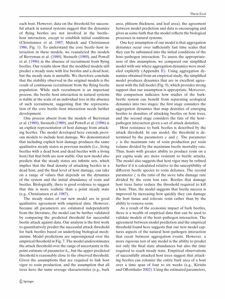
Fig. 7 Predicted threshold for successful attack of Mountain PineBeetles as a function of host vigor (dashed lines). All rate para-meters in the model are estimated independently using literaturedata. The range reflects the uncertainty in the sieve tube lossrate ko. The upper line is ζ = 0.47 and the lower line is ζ = 1.89.Empirical data are shown with circles as in Fig. 1

predicted threshold from the parameterized linearmodel is shown in Fig. 7.

Discussion

The work of Berryman et al. (1989), Stenseth (1989),and Powell et al. (1996) provide the first dynamicmodels of the interaction between bark beetles andhost trees that explicitly describes resin defenses. Thesemodels also include continuous recruitment of flyingbeetles to the population of beetles that are attacking

Table 2 Literatureparameters for the linearmodel

Source details are given inAppendix D

Parameter Description Value Source

Ro Initial resin volume 0.01Rm (l) 1ro Maximum resin concentration 327 (l m−3) 2Rm Maximum resin volume 46.1 (l) 3ho Beetle mortality rate per resin 0.0003869 (l−1 day−1) 4go Resin loss rate per beetle 4.44e-6 (A−1 day−1) 5ko Sieve tube loss rate per beetle 2.1e-6 – 8.4e-6 (A−1 day−1) 6L Leaf area 20 (m2) 7mw Wood production cost 0.305 (g g−1) 8cw Wood mass per carbon mass 1.96 (g g−1) 9mr Resin production cost 0.69 (g g−1) 10cr Resin mass per carbon mass 1.14 (g g−1) 11tr Time conversion to growing days 0.0056 (y day−1) 12δr Resin density 854.7 (g l−1) 13x Phloem thickness 0.015 (m) 14

Theor Ecol

each host. However, data on the threshold for success-ful attack in natural systems suggest that the dynamicsof flying beetles are not involved in the beetle–host interaction, except to establish initial conditions(Christiansen et al. 1987; Mulock and Christiansen1986, Fig. 1). To understand the core beetle–host in-teraction in these models, we reanalyzed the modelsof Berryman et al. (1989), Stenseth (1989), and Powellet al. (1996) in the absence of recruitment from flyingbeetles. Our results show that the modified models stillpredict a steady state with live beetles and a dead host,but the steady state is unstable. We therefore concludethat the stability observed in the original models is theresult of continuous recruitment from the flying beetlepopulation. While such recruitment is an importantprocess, the beetle–host interaction in natural systemsis stable at the scale of an individual tree in the absenceof such recruitment, suggesting that the representa-tion of the core beetle–host interaction needs furtherdevelopment.

One process absent from the models of Berrymanet al. (1989), Stenseth (1989), and Powell et al. (1996) isan explicit representation of host damage from attack-ing beetles. The model developed here extends previ-ous models to include host damage. We demonstratedthat including explicit host damage produces the samequalitative steady states as previous models (i.e., livingbeetles with a dead host and dead beetles with a livinghost) but that both are now stable. Our new model alsopredicts that the steady states are infinite sets, whichimplies that the final density of attacking beetles in adead host, and the final level of host damage, can takeon a range of values that depends on the dynamicsof the system and the initial abundance of resin andbeetles. Biologically, there is good evidence to suggestthat this is more realistic than a point steady state(e.g., Christiansen et al. 1987).

The steady states of our new model are in goodqualitative agreement with empirical data. However,because all parameters are estimated independentlyfrom the literature, the model can be further validatedby comparing the predicted threshold for successfulbeetle attack against data. Our analysis is the first workto quantitatively predict the successful attack thresholdfor bark beetles based on underlying biological mech-anisms. Model predictions are superimposed over theempirical threshold in Fig. 7. The model underestimatesthe attack threshold over the range of uncertainty in thepoint estimate of parameter ko, but the upper predictedthreshold is reasonably close to the observed threshold.Given the assumptions that are required to link hostvigor to resin production, and the assumption that alltrees have the same average characteristics (e.g., bark

area, phloem thickness, and leaf area), the agreementbetween model prediction and data is encouraging andgives us some faith that the model reflects the biologicalprocesses in natural systems.

One key assumption of our model is that aggregationdynamics occur over sufficiently fast time scales thatthey can be subsumed into the initial conditions of thehost–pathogen interaction. To assess the appropriate-ness of this assumption, we compared our simplifiedmodel with one where aggregation dynamics were mod-eled explicitly (Appendix E). Using aggregation dy-namics obtained from an empirical study, the simplifiedmodel produces dynamics that are in excellent agree-ment with the full model (Fig. 9), which provides strongsupport that our assumption is appropriate. Moreover,this comparison indicates how studies of the bark-beetle system can benefit from separating ecologicaldynamics into two stages: the first stage considers theaggregation dynamics that map densities of emergingbeetles to densities of attacking beetles on host trees,and the second stage considers the fate of the host–pathogen interaction given a set of attack densities.

Host resistance to bark beetles is described by theattack threshold. In our model, the threshold is de-termined by the parameters γ and ζ . The parameterγ is the maximum rate of resin production per resinvolume divided by the maximum beetle mortality rate.Thus, hosts with greater ability to produce resin on aper capita scale are more resistant to beetle attacks.The model also suggests that host vigor may be refinedfurther if it is calculated relative to the susceptibility ofdifferent beetle species to resin defenses. The secondparameter ζ is the ratio of the sieve tube damage ratedivided by the resin loss rate. Beetles that damagehost trees faster reduce the threshold required to killa host. Thus, the model suggests that beetle success isimproved by increasing how quickly they can damagethe host tissue and tolerate resin rather than by theability to remove resin.

As a result of the economic impact of bark beetles,there is a wealth of empirical data that can be used tovalidate models of the host–pathogen interaction. Theagreement between model prediction and the empiricalthreshold found here suggests that our new model cap-tures aspects of the natural host–pathogen interactionthat occur between aggregation events. However, amore rigorous test of any model is the ability to predictnot only the final state abundances but also the timerequired to reach steady state. Empirical observationsof successfully attacked host trees suggest that attack-ing beetles can colonize the entire bark area of a hostover a time span of four to six weeks (e.g., Kirisitsand Offenthaler 2002). Using the estimated parameters,

Theor Ecol

the model predicts that the time for half of the barkarea to be damaged is over 200 days, which is muchlonger than the colonization time observed in naturalsystems. Thus, while the model developed here cap-tures the threshold for attack, there still remains scopefor further development. Our present analysis focuseson model predictions using only point estimates of theparameters. As new empirical data become availablefor this system, more robust point estimates can bedeveloped and the analysis can be expanded to incor-porate the variance and covariance in parameter es-timates. Furthermore, by developing resin productionfunctions (Eq. 24) that include more detailed physi-ological processes, the model presented here can beexpanded to consider situations where tree growth islimited by both carbohydrates and nutrients.

The general model developed here describes the fateof the beetle–host interaction through the processes ofresinous defenses and host damage. For a wide classof functions, the model predicts that the steady statesare infinite sets, which is more consistent with empiricalobservations than previous models. The linear versionof the model does reasonably well at predicting the em-pirical threshold when parameterized to independentdata. However, there is clearly room for improvement.In particular, we feel that a better understanding of thefunctions and parameters that describe the biologicalprocesses will be invaluable towards assessing the util-ity of the model proposed here. The advantage of es-tablishing a single framework to investigate beetle–hostsystems is to compare across species that have markedlydifferent success in attacking host trees. For example,are some species less successful because they have lesstendency to aggregate, or because they are less able todamage a host? Because beetle survival is determinedto a large extent by the ability to kill a host tree,the threshold for successful attack generates a strongAllee effect in bark beetles at the population scale.Thus, understanding how the characteristics of eachbeetle species determine the successful attack thresholdwill help us understand and predict the populationdynamics of different bark beetle species.

Acknowledgements We would like to thank Alex Potapov andFrank Hilker for independently solving the phase-plane tra-jectories used in Appendix B, and two anonymous reviewerswho helped improve the manuscript. This study was funded byNatural Resources Canada–Canadian Forest Service under theMountain Pine Beetle Initiative. Publication does not necessarilysignify that the contents of this report reflect the views or policiesof Natural Resources Canada–Canadian Forest Service. Addi-tional support was provided by Natural Sciences and EngineeringResearch Council (NSERC) and Alberta Ingenuity Postdoctoralfellowships to WAN and NSERC Discovery grants and CanadaResearch Chairs to MAL.

Appendix A

In the absence of recruitment, the beetle–host modelpresented by Stenseth (1989) is

dAdt

= −b1 AR (27)

dRdt

= b2 − b3 A − (b4 − b5 A)R (28)

where A(t) is the density of attacking beetles per treeand R(t) is the volume of resin per beetle gallery.Introducing the following dimensionless variables

A = Ab5

b4, R = R

b5

b3, t = tb4

and the dimensionless parameters

α = b1b3

b4b5, β = b5b2

b4b3

we can write the dimensionless version of the modifiedmodel as (after dropping the tildes)

dAdt

= −αAR (29)

dRdt

= β − A − R + AR (30)

The model given by Eqs. 29 and 30 has two steadystates. The first is (A∗, R∗) = (0, β), which is a steadystate where the tree is alive and all attacking beetles aredead. The second is (A∗, R∗) = (β, 0), which is a steadystate where the beetles have successfully killed the hosttree. The Jacobian of Eqs. 29 and 30 is given by

J(A∗,R∗) =( −αR∗ −αA∗

R∗ − 1 A∗ − 1

)

(31)

At the steady state (A∗, R∗) = (0, β), both eigenvaluesare negative, which means that the tree alive steadystate is stable. At the steady state (A∗, R∗) = (β, 0), oneeigenvalue is negative and one is positive. Thus, the treedead steady state is an unstable saddle.

Appendix B

Stability analysis of the Powell et al. (1996) model inthe absence of beetle recruitment (Eqs. 9 and 10). TheJacobian is given by

J(H∗,R∗) =(−R∗ −H∗

−R∗ β − 2β R∗ − H∗

)

(32)

At the steady state (H∗, R∗) = (0, 1), both eigenvaluesare negative and the live host steady state is stable. At

Theor Ecol

the steady state (H∗, R∗) = (H, 0), one of the eigen-values is zero, which means that the eigenvalues areinsufficient for characterizing stability. To investi-gate stability at this steady state, we study the non-linear perturbation equations. Let H(t) = H∗ + h(t)and R(t) = R∗ + r(t), where h(t) and r(t) are small per-turbations around the steady state (H∗, R∗). The per-turbation equations from the steady state (H∗, R∗) =(H, 0) are

dhdt

= −r(H + h) (33)

drdt

= r(β − H − h) − βr2 (34)

We begin by considering the relationship between r andh at the dr/dh = 0 isocline (denoted by r and h).

r = 1 − H + hβ

(35)

Because r ≥ 0 and dh/dt ≤ 0, the phase-plane trajecto-ries always decrease along h. For values of h greaterthan the isocline, dr/dt is negative, and for values ofh less than the isocline, the gradient dr/dt is positive.This can be seen by substituting the point h = h + ε intoEq. 34, which yields

drdt

= −rε (36)

If ε is negative, then r will increase, and if ε is positive,then r will decrease. The isocline given by Eq. 35 crossesthe stable steady state of r = 0 at the point (h, r) = (β −H, 0). The critical trajectory can now be defined as theone that passes through the point (h, r) = (β − H, 0)

because only trajectories with smaller r (or larger h)than this critical trajectory will be in the basin of at-traction of r∗ = 0. The critical trajectory for the systemgiven by Eqs. 9 and 10 can be solved analytically, whichallows us to write the perturbation conditions exactly.By defining η = ln(H + h) and μ = r exp(−βη), we canrewrite Eqs. 33–34 as

dudη

= eη(1−β) − βe−βη (37)

If β �= 1, then the solution of Eq. 37 through the criticalpoint (h, r) = (β − H, 0) is

r = 1

1 − β

⎛

⎝1 − β + H + h −(

H + hβ

)β⎞

⎠ (38)

If β = 1, then the solution is

r = 1 + (H + h)(

ln(H + h) − 1)

(39)

The stability criterion for H at the steady state(H∗, R∗) = (H, 0) can be determined numerically forarbitrary perturbations using Eqs. 38 and 39. As r → 0and h → 0, the stability criterion is H = β.

Appendix C

Stability analysis of the linear host–pathogen modelgiven by Eqs. 16–18. The Jacobian is

J(A∗,S∗,R∗) =⎛

⎝

−R∗ 0 0−ζ S∗ −ζ A∗ 0−R∗ γ (1 − R∗) −γ S∗ − A∗

⎞

⎠ (40)

At each of the three steady states (A∗, S∗, R∗) =(A, 0, 0), (0, 0, R), (0, S, 1), there is at least one zeroeigenvalue, which means that a linear analysis aroundthe steady state is not sufficient to assess stability. Todetermine stability of the steady states, we study thenonlinear perturbations through simulation. The fullperturbation equations for all steady states are

dadt

= −(A∗ + a)(R∗ + r) (41)

dsdt

= −ζ(A∗ + a)(S∗ + s) (42)

drdt

= γ (S∗ + s)(1 − R∗ − r) − (A∗ + a)(R∗ + r) (43)

where a = A − A∗, s = S − S∗, and r = R − R∗ areperturbations around the steady state (A∗, S∗, R∗). Theperturbations surrounding each steady state are ob-tained by setting (A∗, S∗, R∗) = (A, 0, 0), (0, 0, R), or(0, S, 1). Because a and s can only decrease, stabilityfor all steady states is assessed by whether or not rdecays to zero. Unless otherwise noted, we exploredthe parameter space of ζ and γ from zero to 1010 (i.e.,0 ≤ ζ ≤ 1010 and 0 ≤ γ ≤ 1010).

Near the steady state (A∗, S∗, R∗) = (0, S, 1), r de-cays to zero from the initial conditions of (ao, so, ro) =(10−8, 10−8, −10−8) for all values of ζ explored, allvalues of 0 ≤ S ≤ 1, and for values of γ > 0. Thus, weconclude that the steady state (A∗, S∗, R∗) = (0, S, 1) isstable.

Near the steady state (A∗, S∗, R∗) = (0, 0, R), r in-creases to r∗ = 1 − R from the initial conditions of(ao, so, ro) = (10−8, 10−8, 0) for all values of ζ explored,all values of 0.01 ≤ R ≤ 1, and for values of γ > 0.Values of R < 0.01 yielded unreliable numerical sim-ulations for small values of γ . Thus, for γ > 0 andR ≥ 0.01, the steady state (A∗, S∗, R∗) = (0, 0, R) isunstable.

The steady state (A∗, S∗, R∗) = (A, 0, 0) is a littledifferent from the others in that it is locally stable but

Theor Ecol

not globally stable for A bounded away from zero. Fora given set of parameters, a sufficiently small pertur-bation could be found such that r decayed to zero.Specifically, (ao, ro, so) = (0, ε, ε), r decays to zero forε sufficiently small, for 10−10 ≤ ζ ≤ 1010, 0 ≤ γ ≤ 1010,and A ≥ 0.01. We did not check 0 < ζ < 10−10, andvalues of A < 0.01 yielded unreliable numerical simu-lations. Thus, for slightly positive values of ζ and A ≥0.01, the steady state (A∗, S∗, R∗) = (A, 0, 0) is stable.

Appendix D

1. Initial resin density, relative to Rm, is always low(e.g., Raffa and Smalley 1995). We assume Ro =0.01Rm based on Wallin and Raffa (1999).

2. Raffa and Smalley (1995) report a maximummonoterpene concentration of 305 mg per gramof dried phloem. Assuming a resin density of0.858 g ml−1 based on the largest component ofresin α-pinene, a dried phloem density of 0.46 gcm−3 (Bouffier et al. 2003), and a monoterpeneconcentration in resin of 0.5, we estimate a max-imum resin concentration of ro = 327 (l m−3).

3. Maximum resin volume can be estimated fromRm = roxB, where x is phloem thickness and B isbark area. From Waring and Pitman (1985), theaverage bark area was B = 9.4 (m2). Assumingan average phloem thickness of x = 0.015 (m)(e.g. Zausen et al. 2005) gives an estimate of Rm =46.1 (l).

4. Raffa and Berryman (1983) report a 30% beetlemortality rate over a ∼20-day period in host treesthat are killed by mountain pine beetles. If weassume that resin volume was maximal (i.e., Rm),then this gives a rough mortality rate estimate ofho = 0.0003869 (l−1 day−1).

5. From Raffa and Smalley (1995), we can get anestimate for the resin loss rate within the fun-gal/beetle activity zone (gz). Using an initial resinconcentration of 250 mg per gram, and a finalconcentration of 210 mg per gram over a 15-dayperiod, we estimate the loss rate of resin withinthe fungal zone as gz = 0.0116 (A−1 day−1). Toconvert this into a per-capita loss rate of resin overthe entire tree from each attack, we use the sam-pled lesion size of 36 cm2 from Raffa and Smalley(1995), and the average bark area of B = 9.4 (m2)from Waring and Pitman (1985), to estimate aresin loss rate of go = 4.4 × 10−6 (A−1 day−1).

6. The linear growth of the damaged area is roughlybetween 0.5 and 1 cm per day (Reid et al. 1967).Thus, we assume an area increment in the range of

0.196–0.785 cm2 per day of damaged tissue. If weassume that sieve tube damage is best accountedfor by the area of damage per area of bark, then,assuming an average bark area of B = 9.4 (m2)from Waring and Pitman (1985), the sieve tubedamage rate is given by the range of ko = 2.1 ×10−6 to ko = 8.4 × 10−6.

7. Using the average DBH of 0.15 (m) from Waringand Pitman (1985), the sapwood area to DBHrelationship from Bond-Lamberty et al. (2002),and the sapwood area to leaf area relationshipfrom Callaway et al. (1994) for lodgepole pines,we estimate the average leaf area for the site asL = 20 (m2).

8. From Lavigne and Ryan (1997). Value used isaveraged over locations and age classes and agreeswell with the estimate for generic wood of mw =0.25 (Penning de Vries 1975).

9. Czimezik et al. (2002).10. From Gershenzon (1994), the metabolic cost of

producing monoterpenes is 3.54 (g g−1) of glu-cose per monoterpene. Using the molar massof monoterpenes (136.23 g Mol−1) and glucose(180.16 g Mol−1), the total carbon cost by massis 3.2 g glucose per gram of resin. Convertingthis to a dimensionless proportion yields mr =0.69 (g g−1).

11. From the molar mass of monoterpenes(136.23 g Mol−1), cr = 1.14 (g g−1).

12. Assuming a 180-day growing season.13. Using a resin density of 0.858 g ml−1 for pinene,

which is the most abundant component of resin.14. We assume a typical value of x = 0.015 (m) (e.g.,

Zausen et al. 2005).

Appendix E

The model given by Eqs. 16–18 assumes that the time-scale of beetle aggregation to a host tree is sufficientlyfast, relative to the time-scale of the attack dynamics,that the process of aggregation can be subsumed intothe initial conditions of the model (i.e., Ao). To as-sess the validity of this assumption, we can explicitlyincorporate aggregation dynamics and compare thiswith the simplified model. The dimensional model withaggregation dynamics is given by

dAdt

= Ao�(t, α, β) − ho AR (44)

dSdt

= −ko AS (45)

dRdt

= fo

(

1 − RRm

)

S − go AR (46)

Theor Ecol

Fig. 8 Proportion of beetle attacks through time from Raffaand Berryman (1983). Circles are digitized data and lines are fitgamma distribution. Black shows dynamics in 1977, dark graythose in 1978, and light gray those in 1979

where �(t, α, β) describes the proportion of the totalattacking beetles (Ao) that arrive at time t. To parame-terize the aggregation distribution for an empirical ex-

Fig. 9 Dynamics of the attack process for two levels of attackdensity (Ao = 20 and Ao = 50). Black dots show dynamics whenaggregation is explicitly incorporated Eqs. 44–46, and gray linesshow dynamics under the simplifying assumption that aggrega-tion can be subsumed into an initial attack density Ao Eqs. 16–18. Circles denote initial conditions for both models, and arrowsshow the direction of time. Note that the gray lines overlay theblack dots for much of the dynamics. Despite the differing initialconditions, time trajectories of the simplified model approachthat of the full model with explicit aggregation, which suggeststhat the simplified model is a good approximation to the asymp-totic dynamics of the full model well. All other parameter valuesare given in Table 2

ample, we fit the distribution to the arrival data in Fig. 1of Raffa and Berryman (1983). Fitting the functionyields parameter estimates of α = {2.61, 5.21, 3.01} andβ = {0.87, 0.47, 0.96} for the years 1977, 1978, and 1979(Fig. 8). To demonstrate the impact of incorporatingboth time-scales, we use the mean parameter estimatesof α = 3.61 and β = 0.77. Figure 9 shows predicteddynamics of the attack process under both models. Thesimilarity of the dynamics demonstrates that the simpli-fying assumption of subsuming the aggregation processinto an initial condition is a good approximation to thefull model.

References

Allee W (1931) Animal aggregations. The University of ChicagoPress, Chicago

Berryman A (1979) Dynamics of bark beetle populations: analy-sis of dispersal and redistribution. Bull Soc Entomol Suisse52:227–234

Berryman A, Stenseth N (1989) A theoretical basis for under-standing and manaing biological populations with particularreference to the spruce bark beetle. Holarct Ecol 12:387–394

Berryman A, Raffa K, Millstein J, Stenseth N (1989) Interactiondynamics of bark beetle aggregation and conifer defenserates. OIKOS 56:256–263

Bond-Lamberty B, Wang W, Gower S (2002) Aboveground andbelowground biomass and sapwood area allometric equa-tions for six boreal tree species of northern alberta. Can JFor Res 32:1441–1450

Bouffier L, Gartner B, Domec J (2003) Wood densityand hydraulic properties of ponderosa pine from thewillamette valley vs. the cascade mountains. Wood Fiber Sci35(2):217–233

Callaway R, DeLucia E, Schlesinger W (1994) Biomass alloca-tion of montane and desert ponderosa pine: an analog forresponse to climate change. Ecology 75(5):1474–1481

Christiansen E, Waring R, Berryman A (1987) Resistance ofconfiers to bark beetle attack: searching for general relation-ships. For Ecol Manag 22:89–106

Courchamp F, Clutton-Brock T, Grenfell B (1999) Inverse den-sity dependence and the allee effect. Trends Ecol Evol14(10):405–410

Czimezik C, Preston C, Schmidt M, Werner R, Schulze E (2002)Effects of charring on mass, organic carbon, and stablecarbon isotope composition of wood. Org Geochem 33:1207–1223

Franceschi V, Krokene P, Christiansen E, Krekling T (2005)Anatomical and chemical defenses of conifer bark againstbark beetles and other pests. New Phytol 167:353–376

Gershenzon J (1994) Metabolic cost of terpenoid accumulationin higher plants. J Chem Ecol 20(6):1281–1328

Kirisits T, Offenthaler I (2002) Xylem sap flow of norway spruceafter inocluation with the blue stain fungus Ceratocystispolonica. Plant Pathol 51:359–364

Lavigne M, Ryan M (1997) Growth and maintenance respirationrates of aspen, black spruce and jack pine stems at northernand southern boreas sites. Tree Physiol 17:543–551

Lewinsohn E, Gijzen M, Croteau R (1991) Defence mechanismsof conifers. Plant Physiol 96:44–49

Theor Ecol

Logan J, Powell J (2001) Ghost forests, global warming, and themountain pine beetle. Am Entomol 47:160–173

Lombardero ML, Ayres MP, Lorio PL Jr, Ruel JJ (2000) Envi-ronmental effects on constitutive and inducible defences ofPinus taeda. Ecol Lett 3:329–339

Loomis W (1932) Growth-differentiation balance vs.carbohydrate-nitrogen ratio. Proc Am Soc Hortic Sci 29:240–245

Miller R, Berryman A (1986) Carbohydrate allocation andmountain pine beetle attack in girdled lodgepole pines. CanJ For Res 16(5):1036–1040

Mulock P, Christiansen E (1986) The threshold of successful at-tack by Ips typographus on Picea abies: a field experiment.For Ecol Manag 14:125–132

Ogden N, Casey A, French N, Adams J, Woldehiwet Z(2002) Field evidence for density-dependent facilitationamongst Ixodes ricinus ticks feeding on sheep. Parasitology124:117–125

Penning de Vries F (1975) Use of assimilates in higher plants.In: Cooper JP (ed) Photosynthesis and productivity in differ-ent environments. Cambridge Unviersity Press, Cambridge,pp 459–480

Powell J, Logan J, Bentz B (1996) Local projections for aglobal model of mountain pine beetle attacks. J Theor Biol179(3):243–260

Raffa K (2001) Mixed messages across multiple trophic levels:the ecology of bark beetle chemical communication systems.Chemoecology 11:49–65

Raffa K, Berryman A (1983) The role of host plant resistancein the colonization behavior and ecology of bark beetles(coleoptera:scolytidae). Ecol Monogr 53(1):27–49

Raffa K, Smalley E (1995) Interaction of pree-attack andinduced monoterpene concentrations in host conifer de-fense against bark beetle-fungal complexes. Oecologia 102:285–295

Raffa K, Aukema B, Erbilgin N, Klepzig K, Wallin K (2005) In-teractions among conifer terpenoids and bark beeltes acrossmultipls levels of scale: an attempt to understand linksbetween population patterns and physiological processes.Recent Adv Phytochem 39:79–118

Reid R, Whitney H, Watson J (1967) Reactions of lodgepole pineto attack by Dendroctonus ponderosae hopkins and bluestain fungi. Can J Bot 45:1115–1126

Stenseth N (1989) A model for the conquest of a tree by barkbeetles. Holarct Ecol 12:408–414

Thompson M, Holbrook N (2003) Scaling phloem transport:water potential equilibrium and osmoregulatory flow. PlantCell Environ 26:1561–1577

Trapp S, Croteau R (2001) Defensive resin biosynthesis inconifers. Annu Rev Plant Physiol Plant Mol Biol 52:689–724

Turtola A, Manninen A, Rikala R, Kainulainen P (2003) Droughtstress alters the concentration of wood terpenoids in scotspine and norway spruce seedlings. J Chem Ecol 29(9):1981–1995

Uma Devi K, Uma Maheswara Rao C (2006) Allee effect in theinfection dynamics of the entomopathogenic fungus Beave-ria bassiana (bals) vuill. on the beetle, Mylabris pustulata.Mycopathologia 161:385–394

Vanninen P, Mäkelä A (2005) Carbon budget for scots pine trees:effect of size, competition and site fertility on growth alloca-tion and production. Tree Physiol 25:17–30

Wallin K, Raffa K (1999) Altered constitutive and induciblephloem monoterpenes following natural defoliation of jackpine: implications to host mediated interguild interactionsand plant defense theories. J Chem Ecol 25(4):861–880

Wallin K, Raffa K (2001) Effects of folivory on subcortical plantdefenses: can defense theories predict interguild processes?Ecology 82(5):1387–1400

Waring R, Pitman G (1985) Modifying lodgepole pine standsto change susceptibility to mountain pine beetle attack.Ecology 66(3):889–897

Waring R, Thies W, Muscato D (1980) Stem growth per unit ofleaf area: a measure of tree vigor. For Sci 1:112–117

Zausen G, Kolb T, Bailey J, Wagner M (2005) Long-term im-pacts of stand management on ponderosa pine physiologyand bark beetle abundance in northern arizona: a replicatedlandscape study. For Ecol Manag 218:291–305

Zhang Y, Reed D, Cattelino P, Gale M, Jones E, Liechty H,Mroz G (1994) A process-based growth model for youngred pine. For Ecol Manag 69:21–40