http://www.econometricsociety.org/

Econometrica, Vol. 81, No. 5 (September, 2013), 2087–2111

CONNECTED SUBSTITUTES AND INVERTIBILITY OF DEMAND

STEVEN BERRYYale University, New Haven, CT 06520, U.S.A., and NBER and Cowles

Foundation

AMIT GANDHIUniversity of Wisconsin, Madison, WI 53706, U.S.A.

PHILIP HAILEYale University, New Haven, CT 06520, U.S.A., and NBER and Cowles

Foundation

The copyright to this Article is held by the Econometric Society. It may be downloaded,printed and reproduced only for educational or research purposes, including use in coursepacks. No downloading or copying may be done for any commercial purpose without theexplicit permission of the Econometric Society. For such commercial purposes contactthe Office of the Econometric Society (contact information may be found at the websitehttp://www.econometricsociety.org or in the back cover of Econometrica). This statement mustbe included on all copies of this Article that are made available electronically or in any otherformat.

Econometrica, Vol. 81, No. 5 (September, 2013), 2087–2111

CONNECTED SUBSTITUTES AND INVERTIBILITY OF DEMAND

BY STEVEN BERRY, AMIT GANDHI, AND PHILIP HAILE1

We consider the invertibility (injectivity) of a nonparametric nonseparable demandsystem. Invertibility of demand is important in several contexts, including identificationof demand, estimation of demand, testing of revealed preference, and economic the-ory exploiting existence of an inverse demand function or (in an exchange economy)uniqueness of Walrasian equilibrium prices. We introduce the notion of “connectedsubstitutes” and show that this structure is sufficient for invertibility. The connectedsubstitutes conditions require weak substitution between all goods and sufficient strictsubstitution to necessitate treating them in a single demand system. The connected sub-stitutes conditions have transparent economic interpretation, are easily checked, andare satisfied in many standard models. They need only hold under some transformationof demand and can accommodate many models in which goods are complements. Theyallow one to show invertibility without strict gross substitutes, functional form restric-tions, smoothness assumptions, or strong domain restrictions. When the restriction toweak substitutes is maintained, our sufficient conditions are also “nearly necessary” foreven local invertibility.

KEYWORDS: Univalence, injectivity, global inverse, weak substitutes, complements.

1. INTRODUCTION

WE CONSIDER THE INVERTIBILITY (INJECTIVITY) of a nonparametric nonsep-arable demand system. Invertibility of demand is important in several theoret-ical and applied contexts, including identification of demand, estimation of de-mand systems, testing of revealed preference, and economic theory exploitingexistence of an inverse demand function or (in an exchange economy) unique-ness of Walrasian equilibrium prices. We introduce the notion of “connectedsubstitutes” and show that this structure is sufficient for invertibility.

We consider a general setting in which demand for goods 1� � � � � J is charac-terized by

σ(x) = (σ1(x)� � � � �σJ(x)

): X ⊆ R

J → RJ�(1)

where x = (x1� � � � � xJ) is a vector of demand shifters. All other arguments ofthe demand system are held fixed. This setup nests many special cases of in-terest. Points σ(x) might represent vectors of market shares, quantities de-manded, choice probabilities, or expenditure shares. The demand shifters x

1This paper combines and expands on selected material first explored in Gandhi (2008) andBerry and Haile (2009). We have benefitted from helpful comments from Jean-Marc Robin, DonBrown, the referees, and participants in seminars at LSE, UCL, Wisconsin, Yale, the 2011 UCLworkshop on “Consumer Behavior and Welfare Measurement,” and the 2011 “Econometrics ofDemand” conference at MIT. Adam Kapor provided capable research assistance. Financial sup-port from the National Science Foundation is gratefully acknowledged.

© 2013 The Econometric Society DOI: 10.3982/ECTA10135

2088 S. BERRY, A. GANDHI, AND P. HAILE

might be prices, qualities, unobserved characteristics of the goods, or latentpreference shocks. Several examples in Section 2 illustrate.

The connected substitutes structure involves two conditions. First, goodsmust be “weak substitutes” in the sense that, all else equal, an increase in xj

(e.g., a fall in j’s price) weakly lowers demand for all other goods. Second, werequire “connected strict substitution”—roughly, sufficient strict substitutionbetween goods to require treating them in one demand system. These con-ditions have transparent economic interpretation and are easily confirmed inmany standard models. They need only hold under some transformation ofthe demand system and can accommodate many settings with complementarygoods.

The connected substitutes conditions allow us to show invertibility withoutthe functional form restrictions, smoothness assumptions, or strong domain re-strictions relied on previously. We also provide a partial necessity result by con-sidering the special case of differentiable demand. There we show that whenthe weak substitutes condition is maintained, connected strict substitution isnecessary for nonsingularity of the Jacobian matrix. Thus, given weak substi-tutes, connected substitutes is sufficient for global invertibility and “nearly nec-essary” for even local invertibility. A corollary to our two theorems is a newglobal inverse function theorem.

Important to our approach is explicit treatment of a “good 0” whose “de-mand” is defined by the identity

σ0(x) = 1 −J∑

j=1

σj(x)�(2)

Formally, (2) is simply a definition of the function σ0(x). Its interpretation willvary with the application. When demand is expressed in shares (e.g., choiceprobabilities or market shares), good 0 might be a “real” good—for example,a numeraire good, an “outside good,” or a good relative to which utilities arenormalized. The identity (2) will then follow from the fact that shares sum to 1.In other applications, good 0 will be a purely artificial notion introduced onlyas a technical device (see the examples below). This can be useful even whenan outside good is also modeled (see Appendix C).

It is clear from (2) that (1) characterizes the full demand system even whengood 0 is a real good. Nonetheless, explicitly accounting for the demand forgood 0 in this case simplifies imposition of the connected substitutes structureon all goods. When good 0 is an artificial good, including it in the connectedsubstitutes conditions proves useful as well. As will be clear below, it strength-ens the weak substitutes requirement in a natural way while weakening therequirement of connected strict substitution.

Also important to our approach is a potential distinction between the set Xand the subset of this domain on which injectivity of σ is in question. A demandsystem generally will not be injective at points mapping to zero demand for

CONNECTED SUBSTITUTES 2089

some good j. For example, raising good j’s price (lowering xj) at such a pointtypically will not change any good’s demand. So when considering conditionsensuring injectivity, it is natural to restrict attention to the set

X̃ ={x ∈ X :σj(x) > 0 ∀j > 0

}

or even to a strict subset of X̃ —for example, considering only values presentin a given data set, or only positive prices even though σ is defined on all ofRJ (e.g., multinomial logit or probit). Allowing such possibilities, we considerinjectivity of σ on any set

X ∗ ⊆ X

(typically X ∗ ⊆ X̃ ). Rather than starting from the restriction of σ to X ∗, how-ever, it proves helpful to allow X ∗ �= X . For example, one can impose usefulregularity conditions on X with little or no loss (we will assume it is a Carte-sian product). In contrast, assumptions on the shape or topological propertiesof X ∗ implicitly restrict either the function σ or the subset of X̃ on which in-jectivity can be demonstrated. Avoiding such restrictions is one significant wayin which we break from the prior literature.

There is a large literature on the injectivity of real functions, most of it de-veloping conditions ensuring that a locally invertible function is globally invert-ible. This literature goes back at least to Hadamard (1906a, 1906b). Althoughwe cannot attempt a full review here, the monograph of Parthasarathy (1983)provides an extensive treatment, and references to more recent work can befound in, for example, Parthasarathy and Ravindran (2003) and Gowda andRavindran (2000). Local invertibility is itself an open question in many impor-tant demand models, where useful conditions like local strict gross substitutesor local strict diagonal dominance fail because each good substitutes only with“nearby” goods in the product space (several examples below illustrate). Evenwhen local invertibility is given, sufficient conditions for global invertibility inthis literature have proven either inadequate for our purpose (ruling out im-portant models of demand) or problematic in the sense that transparent eco-nomic assumptions delivering these conditions have been overly restrictive oreven difficult to identify.

A central result in this literature is the global “univalence” theorem of Galeand Nikaido (1965). Gale and Nikaido considered a differentiable real func-tion σ with nonsingular Jacobian on X ∗ = X .2 They showed that σ is globallyinjective if X ∗ is a rectangle (a product of intervals) and the Jacobian is every-where a P-matrix (all principal minors are strictly positive). While this resultis often relied on to ensure invertibility of demand, its requirements are often

2Gale and Nikaido (1965) made no distinction between X and X ∗. When these differ, Galeand Nikaido implicitly focused on the restriction of σ to X ∗.

2090 S. BERRY, A. GANDHI, AND P. HAILE

problematic. Differentiability is essential, but fails in some important models.Examples include those with demand defined on a discrete domain (e.g., a gridof prices), random utility models with discrete distributions, or finite mixturesof vertical models. Given differentiability, the P-matrix condition can be diffi-cult to interpret, verify, or derive from widely applicable primitive conditions(see the examples below). Finally, the premise of nonsingular Jacobian on rect-angular X ∗ is often a significant limitation. For example, if x represents pricesand σj(x) = 0, an increase in j’s price has no effect on any good’s demand,implying a singular Jacobian. However, the set X̃ (which avoids σj(x) = 0) isoften not a rectangle. In a market with vertically differentiated goods (e.g.,Mussa and Rosen (1978)), a lower quality good has no demand unless its priceis strictly below that of all higher quality goods. So if −x is the price vector,X̃ generally will not be a rectangle. Other examples include linear demandmodels, models of spatial differentiation (e.g., Salop (1979)), the “pure char-acteristics” model of Berry and Pakes (2007), and the Lancasterian model inAppendix C. When X̃ is not a rectangle, the Gale–Nikaido result can demon-strate invertibility only on a rectangular strict subset of X̃ .

The literature on global invertibility has not been focused on invertibility ofdemand, and we are unaware of any result that avoids the broad limitationsof the Gale–Nikaido result when applied to demand systems. This includesresults based on Hadamard’s classic theorem.3 All require some combinationof smoothness conditions, restrictions on the domain of interest, and restric-tions on the function (or its Jacobian) that are violated by important exam-ples and/or are difficult to motivate with natural economic assumptions.4 Theconnected substitutes conditions avoid these limitations. They have clear in-terpretation and are easily checked based on qualitative features of the de-mand system. They hold in a wide range of models studied in practice andimply injectivity without any smoothness requirement or restriction on theset X ∗.

The plan of the paper is as follows. Section 2 provides several examplesthat motivate our interest, tie our general formulation to more familiar spe-

3See, for example, Palais (1959) or the references in Radulescu and Radulescu (1980).4A few results, starting with Mas-Colell (1979), use additional smoothness conditions to allow

the domain to be any full dimension compact convex polyhedron. However, in applications todemand, the natural domain of interest X̃ can be open, unbounded, and/or nonconvex. Exam-ples include standard models of vertical or horizontal differentiation or the “pure characteris-tics model” of Berry and Pakes (2007). And while the boundaries of X̃ (if they exist) are oftenplanes when utilities are linear in x, this is not a general feature. A less cited result in Gale andNikaido (1965) allows arbitrary convex domain but strengthens the Jacobian condition to requirepositive quasidefiniteness. Positive quasidefiniteness (even weak quasidefiniteness, explored inextensions) is violated on X̃ in prominent demand models, including that of Berry, Levinsohn,and Pakes (1995) when x is (minus) the price vector.

CONNECTED SUBSTITUTES 2091

cial cases, and provide connections to related work. We complete the setup inSection 3 and present the connected substitutes conditions in Section 4. Wegive our main result in Section 5. Section 6 presents a second theorem that un-derlies our partial exploration of necessity, enables us to provide tight links tothe classic results of Hadamard and of Gale and Nikaido, and has additionalimplications of importance to the econometrics of differentiated products mar-kets.

2. EXAMPLES

Estimation of Discrete Choice Demand Models

A large empirical literature uses random utility discrete choice models tostudy demand for differentiated products, building on pioneering work ofMcFadden (1974, 1981), Bresnahan (1981, 1987), and others. Conditional in-direct utilities are normalized relative to that of good 0, often an outside goodrepresenting purchase of goods not explicitly under study. Much of the recentliterature follows Berry (1994) in modeling price endogeneity through a vec-tor of product-specific unobservables x, with each xj shifting tastes for goodj monotonically. Holding observables fixed, σ(x) gives the vector of choiceprobabilities (or market shares). Because each σj is a nonlinear function of theentire vector of unobservables x, invertibility is nontrivial. However, it is essen-tial to standard estimation approaches, including those of Berry, Levinsohn,and Pakes (1995), Berry and Pakes (2007), and Dube, Fox, and Su (2012).5

Berry (1994) provided sufficient conditions for invertibility that include linear-ity of utilities, differentiability of σj(x), and strict gross substitutes.6 We re-lax all three conditions, opening the possibility of developing estimators basedon inverse demand functions for new extensions of standard models, includ-ing semiparametric or nonparametric models (e.g., Gandhi and Nevo (2011),Souza-Rodrigues (2011)).

5The Berry, Levinsohn, and Pakes (1995) estimation algorithm also exploits the fact that, inthe models they considered, σ is surjective at all parameter values. Given injectivity, this ensuresthat even at wrong (i.e., trial) parameter values, the observed choice probabilities can be inverted.This property is not necessary for all estimation methods or for other purposes motivating interestin the inverse. However, Gandhi (2010) provided sufficient conditions for a nonparametric modeland also discussed a solution algorithm.

6Although Berry (1994) assumed strict gross substitutes, his proof only required that eachinside good strictly substitute to the outside good. Hotz and Miller (1993) provided an invertibilitytheorem for a similar class of models, although they provided a complete proof only for local, notglobal, invertibility. Berry and Pakes (2007) stated an invertibility result for a discrete choicemodel relaxing some assumptions in Berry (1994), while still assuming the linearity of utilityin xj . Their proof is incomplete, although adding the second of our two connected substitutesconditions would correct this deficiency.

2092 S. BERRY, A. GANDHI, AND P. HAILE

Nonparametric Identification of Demand

Separate from practical estimation issues, there has been growing interestin the question of whether demand models in the spirit of Berry, Levinsohn,and Pakes (1995) are identified without the strong functional form and distri-butional assumptions typically used in applications. Berry and Haile (2010a,2010b) have recently provided affirmative answers for nonparametric mod-els in which x is a vector of unobservables reflecting latent tastes in a marketand/or unobserved characteristics of the goods in a market. Conditioning on allobservables, one obtains choice probabilities of the form (1). The invertibilityresult below provides an essential lemma for many of Berry and Haile’s identi-fication results, many of which extend immediately to any demand system sat-isfying the connected substitutes conditions. Related work includes Chiapporiand Komunjer (2009), which imposed functional form and support conditionsensuring that invertibility follows from the results of Gale and Nikaido (1965)or Hadamard (Palais (1959)).

Inverting for Preference Shocks in Continuous Demand Systems

Beckert and Blundell (2008) recently considered a model in which utilityfrom a bundle of consumption quantities q = (q0� � � � � qJ) is given by a strictlyincreasing C2 function u(q�x), with x ∈ RJ denoting latent demand shocks.The price of good 0 is normalized to 1. Given total expenditure m and pricesp = (p1� � � � �pJ) for the remaining goods, quantities demanded are given byqj = hj(p�m�x) j = 1� � � � � J, with q0 = m − ∑

j>0 pjqj . Beckert and Blundell(2008) considered invertibility of this demand system in the latent vector x,pointing out that this is a necessary step toward identification of demand ortesting of stochastic revealed preference restrictions (e.g., Block and Marschak(1960), McFadden and Richter (1971, 1990), Falmagne (1978), McFadden(2004)). They provided several invertibility results. One requires marginal ratesof substitution between good 0 and goods j > 0 to be multiplicatively separa-ble in x, with an invertible matrix of coefficients. Alternatively, they providedconditions (on functional form and/or derivative matrices of marginal rates ofsubstitution) implying the Gale–Nikaido Jacobian requirement. We provide analternative to such restrictions.

One way to translate their model to ours is through expenditure shares. Todo this, fix p and m, let σj(x) = pjh(p�m�x)/m for j > 0. Expenditure sharessum to 1, implying the identity (2). Other transformations are also possible (seeExample 1 below). And although Beckert and Blundell represented all goodsin the economy by j = 0�1� � � � � J, a common alternative is to consider demandfor a more limited set of goods—for example, those in a particular product cat-egory. In that case, there will no longer be a good whose demand is determinedfrom the others’ through the budget constraint, and it will be natural to havea demand shock xj for every good j. This situation is also easily accommo-dated. Holding prices and all other demand shifters fixed, let σj(x) now give

CONNECTED SUBSTITUTES 2093

the quantity of good j demanded for j = 1� � � � � J. To complete the mapping toour model, let (2) define the object σ0(x). A hint at the role this artificial good0 plays below can be seen by observing that a rise in σ0(x) represents a fall inthe demand for goods j > 0 as a whole.

Existence of Inverse Demand, Uniqueness of Walrasian Equilibrium

Let −xj be the price of good j. Conditional on all other demand shifters,let σj(x) give the quantity demanded of good j. A need for invertible demandarises in several contexts. In an exchange economy, invertibility of aggregateWalrasian demand is equivalent to uniqueness of Walrasian equilibrium prices.Our connected substitutes assumptions relax the strict gross substitutes prop-erty that is a standard sufficient condition for uniqueness. In a partial equi-librium setting, invertibility of aggregate Marshallian demand is required forcompetition in quantities to be well defined. The result of Gale and Nikaido(1965) has often been employed to show uniqueness. Cheng (1985) providedeconomically interpretable sufficient conditions, showing that the Gale andNikaido (1965) Jacobian condition holds under the dominant diagonal condi-tion of McKenzie (1960) and a restriction to strict gross substitutes. In additionto the limitations of requiring differentiability and, especially, a rectangulardomain, the requirement of strict gross substitutes (here and in several otherresults cited above) rules out many standard models of differentiated products,where substitution is only “local,” that is, between goods that are adjacent inthe product space (see, e.g., Figure 1 and Appendix A below). Our invertibil-ity result avoids these limitations. Here we would again use the identity (2) tointroduce an artificial good 0 as a technical device.

3. MODEL

We consider a demand system characterized by (1). Recall that x ∈ X ⊆ RJ

is a vector of demand shifters and that all other determinants of demand areheld fixed.7 Although we refer to σ as “demand” (and to σj(x) as “demandfor good j”), σ may be any transformation of the demand system, for example,σ(x) = g ◦ f (x), where f (x) gives quantities demanded and g : f (X )→ RJ . Inthis case, σ is injective only if f is. Our connected substitutes assumptions onσ are postponed to the following section; however, one should think of xj asa monotonic shifter of demand for good j. In the examples above, xj is either(minus) the price of good j, the unobserved quality of good j, or a shock totaste for good j. In all of these examples, monotonicity is a standard property.Let J = {0�1� � � � � J}. Recall that we seek injectivity of σ on X ∗ ⊆ X , and thatwe have defined the auxiliary function σ0(x) in (2).

7When good 0 is a real good relative to which prices or utilities are normalized, this includesall characteristics of this good. For example, we do not rule out the possibility that good 0 has aprice x0, but are holding it fixed (e.g., at 1).

2094 S. BERRY, A. GANDHI, AND P. HAILE

ASSUMPTION 1: X is a Cartesian product.

This assumption can be relaxed (see Berry, Gandhi, and Haile (2011) fordetails) but appears to be innocuous in most applications. We contrast thiswith Gale and Nikaido’s assumption that X ∗ is a rectangle. There is a superfi-cial similarity, since a rectangle is a special case of a Cartesian product. But afundamental distinction is that we place no restriction on the set X ∗ (see thediscussion in the Introduction). Further, Assumption 1 plays the role of a reg-ularity condition here, whereas rectangularity of X ∗ is integral to the proof ofGale and Nikaido’s result (see also Moré and Rheinboldt (1973)) and limits itsapplicability.

4. CONNECTED SUBSTITUTES

Our main requirement for invertibility is a pair of conditions characterizingconnected substitutes. The first is that the goods are weak substitutes in x inthe sense that when xj increases (e.g., j’s price falls), demand for goods k �= jdoes not increase.

ASSUMPTION 2—Weak Substitutes: σj(x) is weakly decreasing in xk for allj ∈ {0�1� � � � � J}, k /∈ {0� j}.

We make three comments on this restriction. First, in a discrete choicemodel, it is implied by the standard assumptions that xj is excluded from theconditional indirect utilities of goods k �= j and that the conditional indirectutility of good j is increasing in xj .

Second, although Assumption 2 appears to rule out complements, it doesnot. In the case of indivisible goods, demand for complements can be rep-resented as arising from a discrete choice model in which every bundle is adistinct choice (e.g., Gentzkow (2004)). As already noted, the weak substitutescondition is mild in a discrete choice demand system. In the case of divisiblegoods, the fact that σ may be any transformation of the demand system en-ables Assumption 2 to admit some models of complements, including somewith arbitrarily strong complementarity. Example 1 below illustrates.

Finally, consider the relation of this assumption to a requirement of strictgross substitutes. If good zero is a real good, then our weak substitutes con-dition is weaker, corresponding to the usual notion of weak gross substitutes.When good 0 is an artificial good, Assumption 2 strengthens the weak grosssubstitutes condition in a natural way: taking the case where x is (minus) price,all else equal, a fall in the price of some good j > 0 cannot cause the totaldemand (over all goods) to fall.

To state the second condition characterizing connected substitutes, we firstdefine a directional notion of (strict) substitution.

CONNECTED SUBSTITUTES 2095

DEFINITION 1: Good j substitutes to good k at x if σk(x) is strictly decreasingin xj .

Consider a decline in xj with all else held fixed. By Assumption 2, this weaklyraises σk(x) for all k �= j. The goods to which j substitutes are those whosedemands σk(x) strictly rise. When xj is (minus) the price of good j, this isa standard notion. Definition 1 merely extends this notion to other demandshifters that may play the role of x. Although this is a directional notion, inmost examples it is symmetric; that is, j substitutes to k if and only if (iff)k substitutes to j.8 An exception is substitution to good 0: since any demandshifters for good 0 are held fixed, Definition 1 does not define substitution fromgood 0 to other goods.9

It will be useful to represent substitution among the goods with the directedgraph of a matrix Σ(x) whose elements are

Σj+1�k+1 ={

1{good j substitutes to good k at x}� j > 0�0� j = 0�

The directed graph of Σ(x) has nodes (vertices) representing each good and adirected edge from node k to node � whenever good k substitutes to good �at x.

ASSUMPTION 3—Connected Strict Substitution: For all x ∈ X ∗, the directedgraph of Σ(x) has, from every node k �= 0, a directed path to node 0.

Figure 1 illustrates the directed graphs of Σ(x) at generic x ∈ X̃ for somestandard models of differentiated products, letting −x be the price vectorand assuming (as usual) that each conditional indirect utility is strictly de-creasing in price. The connected substitutes conditions hold for X ∗ ⊆ X̃ inall of these models. As panel (e) illustrates, they hold even when J is com-posed of independent goods and either an outside good or an artificial good 0.Each of these examples has an extension to models of discrete/continuous de-mand (e.g., Novshek and Sonnenschein (1979), Hanemann (1984), Dubin andMcFaden (1984)), models of multiple discrete choice (e.g., Hendel (1999),Dube (2004)), and models of differentiated products demand (e.g., Deneckereand Rothschild (1992), Perloff and Salop (1985)) that provide a foundationfor representative consumer models of monopolistic competition (e.g., Spence

8See, for example, Berry, Gandhi, and Haile (2011). We emphasize that this refers to symmetryof the binary notion of substitution defined above, not to symmetry of any magnitudes.

9If good 0 is a real good designated to normalize utilities or prices, one can imagine expandingx to include x0 and defining substitution from good 0 to other goods prior to the normalizationthat fixes x0. If Assumption 3, below, holds under the original designation of good 0, it will holdfor all designations of good 0 as long as substitution (using the expanded vector x = (x0� � � � xJ))is symmetric (in the sense discussed above).

2096 S. BERRY, A. GANDHI, AND P. HAILE

FIGURE 1.—Directed graphs of Σ(x) for x ∈ X̃ (x equals minus price) in some standard mod-els of differentiated products. Panel (a): multinomial logit, multinomial probit, mixed logit, etc.;Panel (b): models of pure vertical differentiation, (e.g., Mussa and Rosen (1978), Bresnahan(1981), etc.); Panel (c): Salop (1979) with random utility for the outside good; Panel (d): Rochetand Stole (2002); Panel (e): independent goods with either an outside good or an artificialgood 0.

CONNECTED SUBSTITUTES 2097

(1976), Dixit and Stiglitz (1977)).10 Note that only the models represented inpanel (a) satisfy strict gross substitutes.

As we have noted already, allowing complementarity is straightforward withindivisible goods. Further, natural restrictions such as additive or subadditivebundle pricing would only help ensure invertibility by restricting the set X ∗.11

The following example shows that complements can be accommodated even insome models of demand for divisible goods.

EXAMPLE 1—Demand for Divisible Complements: Let qj(p) : R+ → R+denote a differentiable function giving the quantity of good j demanded atprice vector p (here x = −p). Let q0(p) = q0 be a small positive constantand define Q(p) = ∑J

j=0 qj(p). Let εjk(p) denote the elasticity of demand forgood j with respect to pk and let εQk(p) denote that of Q(p) with respectto pk. If we assume that, for all p such that qj(p) > 0, (i) Q(p) is strictlydecreasing in pj ∀j ≥ 1, and (ii) εjk(p) ≥ εQk(p) ∀k� j �= k, then it is easilyconfirmed that the connected substitutes conditions hold for any X ∗ ⊆ X̃ un-der the transformation of demand to “market shares” σj(p) = qj(p)

Q(p)(see Ap-

pendix B). A simple example is the constant elasticity demand system in whichqj(p) = Ap−α

j

∏k �=j p

−βk with α > β > 0. For sufficiently small q0 and any X ∗

such that all qj are bounded away from zero, conditions (i) and (ii) above areeasily confirmed (see Appendix B).

The following lemma provides a useful reinterpretation of Assumption 3.

LEMMA 1: Assumption 3 holds iff, for all x ∈ X ∗ and any nonempty K ⊆{1� � � � � J}, there exist k ∈ K and � /∈ K such that σ�(x) is strictly decreasing in xk.

PROOF: (Necessity of Assumption 3) Let I0(x) ⊆ J be composed of 0 andthe indexes of all other goods whose nodes have a directed path to node 0 inthe directed graph of Σ(x). If Assumption 3 fails, then, for some x ∈ X ∗, theset K = J \ I0(x) is nonempty. Further, by construction, there is no directed

10Mosenson and Dror (1972) used a graphical representation to characterize the possible pat-terns of substitution for Hicksian demand. Suppose x is minus the price vector, expanded toinclude the price of good zero (see footnote 9). Suppose further that σ is differentiable and repre-sents the Hicksian (compensated) demand of an individual consumer. Let Σ+(x) be the expandedsubstitution matrix, with elements Σ+

j+1�k+1 = 1{good j substitutes to good k at x}. Mosenson andDror (1972) showed that the directed graph of Σ+(x) must be strongly connected. This is a suffi-cient condition for Assumption 3.

11In a recent paper, Azevedo, White, and Weyl (2013) considered an exchange economy withindivisible goods and a continuum of financially unconstrained consumers with quasilinear utili-ties. They focused on existence of Walrasian equilibrium prices, but also considered uniquenessunder a restriction to additive pricing of the elementary goods in each bundle. Their “large sup-port” assumption on preferences makes all bundles strict gross substitutes in the aggregate de-mand function. See the related discussion in Section 2.

2098 S. BERRY, A. GANDHI, AND P. HAILE

path from any node in K to any node in I0(x). Thus, there do not exist k ∈ Kand � /∈ K such that σ�(x) is strictly decreasing in xk.

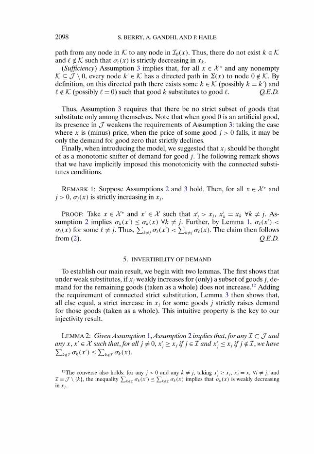
(Sufficiency) Assumption 3 implies that, for all x ∈ X ∗ and any nonemptyK ⊆ J \ 0, every node k′ ∈ K has a directed path in Σ(x) to node 0 /∈ K. Bydefinition, on this directed path there exists some k ∈ K (possibly k = k′) and� /∈ K (possibly �= 0) such that good k substitutes to good �. Q.E.D.

Thus, Assumption 3 requires that there be no strict subset of goods thatsubstitute only among themselves. Note that when good 0 is an artificial good,its presence in J weakens the requirements of Assumption 3: taking the casewhere x is (minus) price, when the price of some good j > 0 falls, it may beonly the demand for good zero that strictly declines.

Finally, when introducing the model, we suggested that xj should be thoughtof as a monotonic shifter of demand for good j. The following remark showsthat we have implicitly imposed this monotonicity with the connected substi-tutes conditions.

REMARK 1: Suppose Assumptions 2 and 3 hold. Then, for all x ∈ X ∗ andj > 0, σj(x) is strictly increasing in xj .

PROOF: Take x ∈ X ∗ and x′ ∈ X such that x′j > xj , x′

k = xk ∀k �= j. As-sumption 2 implies σk(x

′) ≤ σk(x) ∀k �= j. Further, by Lemma 1, σ�(x′) <

σ�(x) for some � �= j. Thus,∑

k �=j σ�(x′) <

∑k �=j σ�(x). The claim then follows

from (2). Q.E.D.

5. INVERTIBILITY OF DEMAND

To establish our main result, we begin with two lemmas. The first shows thatunder weak substitutes, if xj weakly increases for (only) a subset of goods j, de-mand for the remaining goods (taken as a whole) does not increase.12 Addingthe requirement of connected strict substitution, Lemma 3 then shows that,all else equal, a strict increase in xj for some goods j strictly raises demandfor those goods (taken as a whole). This intuitive property is the key to ourinjectivity result.

LEMMA 2: Given Assumption 1, Assumption 2 implies that, for any I ⊂ J andany x�x′ ∈ X such that, for all j �= 0, x′

j ≥ xj if j ∈ I and x′j ≤ xj if j /∈ I , we have∑

k/∈I σk(x′)≤ ∑

k/∈I σk(x).

12The converse also holds: for any j > 0 and any k �= j, taking x′j ≥ xj , x′

i = xi ∀i �= j, andI = J \ {k}, the inequality

∑k/∈I σk(x

′) ≤ ∑k/∈I σk(x) implies that σk(x) is weakly decreasing

in xj .

CONNECTED SUBSTITUTES 2099

PROOF: Let x̃ be such that, for all j �= 0, x̃j = xj if j ∈ I and x̃j = x′j if j /∈ I .

If J \ I contains only 0, then x̃= x and∑k/∈I

σk(x̃)≤∑j /∈I

σk(x)(3)

trivially. If, instead, J \ I contains any nonzero element, without loss let thesebe 1� � � � � n. Then let x̃(0) = x, r = 0, and consider the following iterative ar-gument. Add 1 to r and, for all j > 0, let x̃(r)

j = x̃(r−1)j + 1{j = r}(x′

j − xj). As-sumption 1 ensures that σ is defined at x̃(r) = (x̃(r)

1 � � � � � x̃(r)J ). By Assumption 2,∑

j∈I σj(x̃(r)) ≥ ∑

j∈I σj(x̃(r−1)). Iterating until r = n and recalling the identity

(2), we obtain (3). A parallel argument shows that∑k/∈I

σk

(x′) ≤

∑k/∈I

σk(x̃)�

and the result follows. Q.E.D.

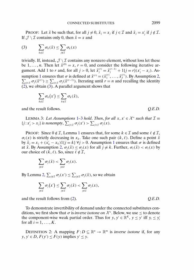
LEMMA 3: Let Assumptions 1–3 hold. Then, for all x�x′ ∈ X ∗ such that I ≡{j :x′

j > xj} is nonempty,∑

j∈I σj(x′) >

∑j∈I σj(x).

PROOF: Since 0 /∈ I , Lemma 1 ensures that, for some k ∈ I and some � /∈ I ,σ�(x) is strictly decreasing in xk. Take one such pair (k� �). Define a point x̃by x̃j = xj + (x′

k − xk)1{j = k} ∀j > 0. Assumption 1 ensures that σ is definedat x̃. By Assumption 2, σj(x̃) ≤ σj(x) for all j �= k. Further, σ�(x̃) < σ�(x) byour choice of (k� �). So, since � /∈ I ,

∑j /∈I

σj(x̃) <∑j /∈I

σj(x)�

By Lemma 2,∑

j /∈I σj(x′)≤ ∑

j /∈I σj(x̃), so we obtain

∑j /∈I

σj

(x′) ≤

∑j /∈I

σj(x̃) <∑j /∈I

σj(x)�

and the result follows from (2). Q.E.D.

To demonstrate invertibility of demand under the connected substitutes con-ditions, we first show that σ is inverse isotone on X ∗. Below, we use ≤ to denotethe component-wise weak partial order. Thus for y� y ′ ∈ RK , y ≤ y ′ iff yi ≤ y ′

i

for all i = 1� � � � �K.

DEFINITION 2: A mapping F :D ⊆ Rn → Rm is inverse isotone if, for anyy� y ′ ∈D, F(y ′) ≤ F(y) implies y ′ ≤ y .

2100 S. BERRY, A. GANDHI, AND P. HAILE

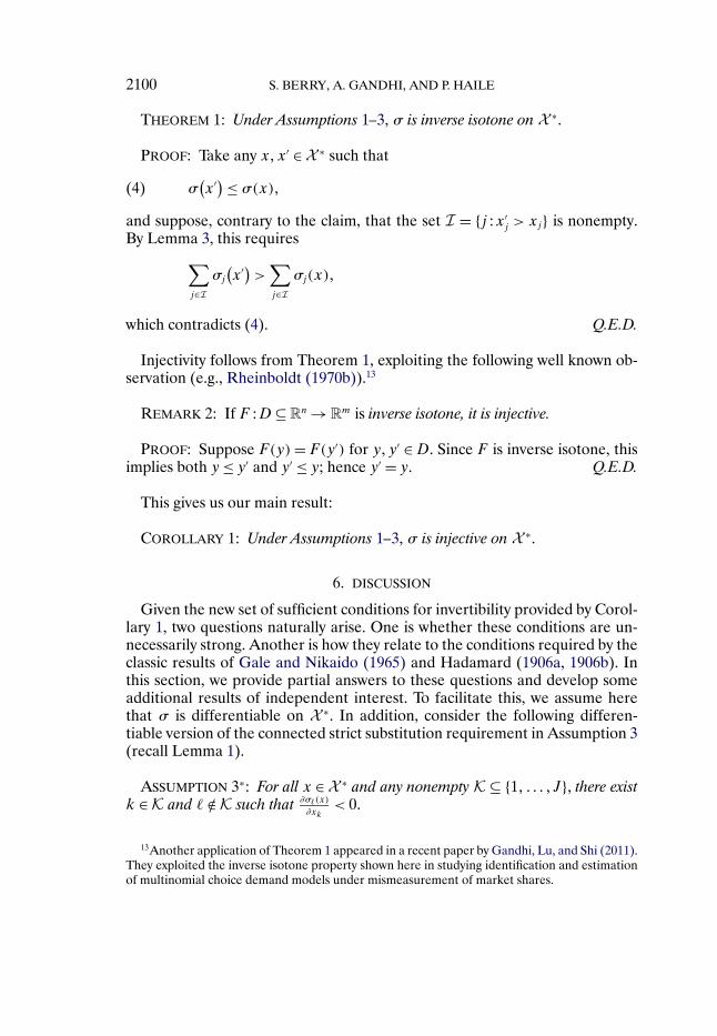
THEOREM 1: Under Assumptions 1–3, σ is inverse isotone on X ∗.

PROOF: Take any x�x′ ∈ X ∗ such that

σ(x′) ≤ σ(x)�(4)

and suppose, contrary to the claim, that the set I = {j :x′j > xj} is nonempty.

By Lemma 3, this requires∑j∈I

σj

(x′) >∑

j∈I

σj(x)�

which contradicts (4). Q.E.D.

Injectivity follows from Theorem 1, exploiting the following well known ob-servation (e.g., Rheinboldt (1970b)).13

REMARK 2: If F :D⊆ Rn → Rm is inverse isotone, it is injective.

PROOF: Suppose F(y) = F(y ′) for y� y ′ ∈ D. Since F is inverse isotone, thisimplies both y ≤ y ′ and y ′ ≤ y; hence y ′ = y . Q.E.D.

This gives us our main result:

COROLLARY 1: Under Assumptions 1–3, σ is injective on X ∗.

6. DISCUSSION

Given the new set of sufficient conditions for invertibility provided by Corol-lary 1, two questions naturally arise. One is whether these conditions are un-necessarily strong. Another is how they relate to the conditions required by theclassic results of Gale and Nikaido (1965) and Hadamard (1906a, 1906b). Inthis section, we provide partial answers to these questions and develop someadditional results of independent interest. To facilitate this, we assume herethat σ is differentiable on X ∗. In addition, consider the following differen-tiable version of the connected strict substitution requirement in Assumption 3(recall Lemma 1).

ASSUMPTION 3∗: For all x ∈ X ∗ and any nonempty K ⊆ {1� � � � � J}, there existk ∈ K and � /∈ K such that ∂σ�(x)

∂xk< 0.

13Another application of Theorem 1 appeared in a recent paper by Gandhi, Lu, and Shi (2011).They exploited the inverse isotone property shown here in studying identification and estimationof multinomial choice demand models under mismeasurement of market shares.

CONNECTED SUBSTITUTES 2101

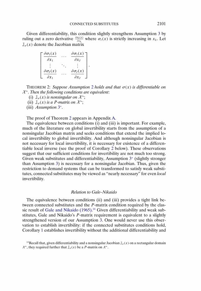
Given differentiability, this condition slightly strengthens Assumption 3 byruling out a zero derivative ∂σ�(x)

∂xkwhere σ�(x) is strictly increasing in xk. Let

Jσ(x) denote the Jacobian matrix

⎡⎢⎢⎢⎢⎣

∂σ1(x)

∂x1· · · ∂σ1(x)

∂xJ���

� � ����

∂σJ(x)

∂x1· · · ∂σJ(x)

∂xJ

⎤⎥⎥⎥⎥⎦ �

THEOREM 2: Suppose Assumption 2 holds and that σ(x) is differentiable onX ∗. Then the following conditions are equivalent:

(i) Jσ(x) is nonsingular on X ∗;(ii) Jσ(x) is a P-matrix on X ∗;(iii) Assumption 3∗.

The proof of Theorem 2 appears in Appendix A.The equivalence between conditions (i) and (iii) is important. For example,

much of the literature on global invertibility starts from the assumption of anonsingular Jacobian matrix and seeks conditions that extend the implied lo-cal invertibility to global invertibility. And although nonsingular Jacobian isnot necessary for local invertibility, it is necessary for existence of a differen-tiable local inverse (see the proof of Corollary 2 below). These observationssuggest that our sufficient conditions for invertibility are not much too strong.Given weak substitutes and differentiability, Assumption 3∗ (slightly strongerthan Assumption 3) is necessary for a nonsingular Jacobian. Thus, given therestriction to demand systems that can be transformed to satisfy weak substi-tutes, connected substitutes may be viewed as “nearly necessary” for even localinvertibility.

Relation to Gale–Nikaido

The equivalence between conditions (ii) and (iii) provides a tight link be-tween connected substitutes and the P-matrix condition required by the clas-sic result of Gale and Nikaido (1965).14 Given differentiability and weak sub-stitutes, Gale and Nikaido’s P-matrix requirement is equivalent to a slightlystrengthened version of our Assumption 3. One would never use this obser-vation to establish invertibility: if the connected substitutes conditions hold,Corollary 1 establishes invertibility without the additional differentiability and

14Recall that, given differentiability and a nonsingular Jacobian Jσ(x) on a rectangular domainX ∗, they required further that Jσ(x) be a P-matrix on X ∗�

2102 S. BERRY, A. GANDHI, AND P. HAILE

domain restrictions Gale and Nikaido required. However, Theorem 2 clari-fies the relationship between the two results.15 One interpretation is that wedrop Gale and Nikaido’s differentiability requirement, replace their restric-tion to rectangular X ∗ with the weak substitutes condition, and replace theirconditions on the Jacobian with the more easily interpreted and slightly weakerrequirement of connected strict substitution.

A Global Inverse Function Theorem

A corollary to our two theorems is the following result.

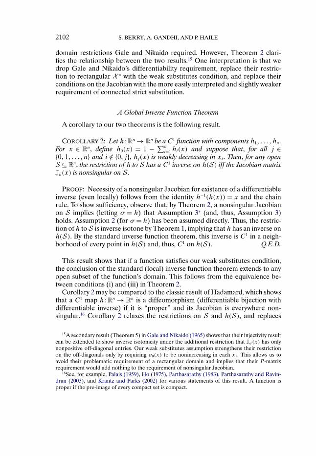
COROLLARY 2: Let h : Rn → Rn be a C1 function with components h1� � � � �hn.For x ∈ Rn, define h0(x) = 1 − ∑n

i=1 hi(x) and suppose that, for all j ∈{0�1� � � � � n} and i /∈ {0� j}, hj(x) is weakly decreasing in xi. Then, for any openS ⊆ Rn, the restriction of h to S has a C1 inverse on h(S) iff the Jacobian matrixJh(x) is nonsingular on S .

PROOF: Necessity of a nonsingular Jacobian for existence of a differentiableinverse (even locally) follows from the identity h−1(h(x)) = x and the chainrule. To show sufficiency, observe that, by Theorem 2, a nonsingular Jacobianon S implies (letting σ = h) that Assumption 3∗ (and, thus, Assumption 3)holds. Assumption 2 (for σ = h) has been assumed directly. Thus, the restric-tion of h to S is inverse isotone by Theorem 1, implying that h has an inverse onh(S). By the standard inverse function theorem, this inverse is C1 in a neigh-borhood of every point in h(S) and, thus, C1 on h(S). Q.E.D.

This result shows that if a function satisfies our weak substitutes condition,the conclusion of the standard (local) inverse function theorem extends to anyopen subset of the function’s domain. This follows from the equivalence be-tween conditions (i) and (iii) in Theorem 2.

Corollary 2 may be compared to the classic result of Hadamard, which showsthat a C1 map h : Rn → Rn is a diffeomorphism (differentiable bijection withdifferentiable inverse) if it is “proper” and its Jacobian is everywhere non-singular.16 Corollary 2 relaxes the restrictions on S and h(S), and replaces

15A secondary result (Theorem 5) in Gale and Nikaido (1965) shows that their injectivity resultcan be extended to show inverse isotonicity under the additional restriction that Jσ(x) has onlynonpositive off-diagonal entries. Our weak substitutes assumption strengthens their restrictionon the off-diagonals only by requiring σ0(x) to be nonincreasing in each xj . This allows us toavoid their problematic requirement of a rectangular domain and implies that their P-matrixrequirement would add nothing to the requirement of nonsingular Jacobian.

16See, for example, Palais (1959), Ho (1975), Parthasarathy (1983), Parthasarathy and Ravin-dran (2003), and Krantz and Parks (2002) for various statements of this result. A function isproper if the pre-image of every compact set is compact.

CONNECTED SUBSTITUTES 2103

properness with the weak substitutes condition. Whereas properness is not eas-ily verified, we have shown that weak substitutes is a natural property of manydemand systems.

Unlike Hadamard’s theorem and its variations, Corollary 2 avoids the ques-tion of surjectivity. Rheinboldt (1970a) provided necessary and sufficient con-ditions for surjectivity onto Rn for inverse isotone functions.

Transforming Demand

As noted already, if f (x) describes a demand system that does not itself sat-isfy the connected substitutes conditions, it may be possible to find a functiong such that σ = g ◦ f does. The equivalence of conditions (i) and (iii) in The-orem 2 provides some guidance on suitable transformations g. Suppose thatboth f and g are differentiable with nonsingular Jacobians. Then if σ satisfiesweak substitutes, it also satisfies connected substitutes.

Identification and Estimation in Differentiated Products Markets

The sufficiency of condition (iii) for conditions (i) and (ii) in Theorem 2is important to the econometric theory underlying standard empirical modelsof differentiated products markets (e.g., Berry, Levinsohn, and Pakes (1995)).Berry and Haile (2010a) used the latter implication to establish nonparametricidentifiability of firms’ marginal costs and the testability of alternative mod-els of oligopoly competition. There the P-matrix property ensures invertibil-ity of the derivative matrix of market shares with respect to prices for goodsproduced by the same firm—a matrix appearing in the first-order conditionscharacterizing equilibrium behavior. Their results generalize immediately tomodels with continuous demand satisfying connected substitutes.

Berry, Linton, and Pakes (2004) provided the asymptotic distribution theoryfor a class of estimators for discrete choice demand models. A key condition,confirmed there for special cases, is that the Jacobian of the demand system(with respect to a vector of demand shocks) is full rank on X ∗. Sufficiencyof the connected substitutes conditions establishes economically interpretablesufficient conditions with wide applicability.

7. CONCLUSION

We have introduced the notion of connected substitutes and shown thatthis structure is sufficient for invertibility of a nonparametric nonsepara-ble demand system. The connected substitutes conditions are satisfied in awide range of models used in practice, including many with complementarygoods. These conditions have transparent economic interpretation, are easilychecked, and allow demonstration of invertibility without functional form re-strictions, smoothness assumptions, or strong domain restrictions commonly

2104 S. BERRY, A. GANDHI, AND P. HAILE

relied on previously. Further, given a restriction to weak substitutes, our suffi-cient conditions are also “nearly necessary” for even local invertibility.

APPENDIX A: PROOF OF THEOREM 2

We first review some definitions (see, e.g., Horn and Johnson (1990)).A square matrix is reducible if it can be placed in block upper triangular formby simultaneous permutations of rows and columns. A square matrix that isnot reducible is irreducible. A square matrix A with elements aij is (weakly)diagonally dominant17 if, for all j,

|ajj| ≥∑i �=j

|aij|�

If the inequality is strict for all j, A is said to be strictly diagonally dominant. Anirreducibly diagonally dominant matrix is a square matrix that is irreducible andweakly diagonally dominant, with at least one diagonal being strictly dominant,that is, with at least one column j such that

|ajj|>∑i �=j

|aij|�(A.1)

We begin with three lemmas concerning square matrices. The first is wellknown (see, e.g., Taussky (1949) or Horn and Johnson (1990, p. 363)) and thethird is a variation on a well known result. The second appears to be new.

LEMMA 4: An irreducibly diagonally dominant matrix is nonsingular.

LEMMA 5: Let D be a square matrix with nonzero diagonal entries and supposethat every principal submatrix of D is weakly diagonally dominant, with at leastone strictly dominant diagonal. Then D is nonsingular.

PROOF: Let M = D and consider the following iterative argument. If M is1 × 1, nonsingularity is immediate from the nonzero diagonal. For M of higherdimension, if M is irreducible, the result follows from Lemma 4. Otherwise,M is reducible, so by simultaneous permutation of rows and columns, it can beplaced in block upper triangular form; that is, for some permutation matrix P ,

M∗ ≡ PMP ′ =[A B0 C

]�

where A and C are square matrices. Simultaneous permutation of rows andcolumns changes neither the set of diagonal entries nor the off-diagonal en-tries appearing in the same column (or row) as a given diagonal entry. Further,

17Here we refer to column dominance, not row dominance.

CONNECTED SUBSTITUTES 2105

each principal submatrix of A or of C is also a principal submatrix of D (pos-sibly up to simultaneous permutation of rows and columns). Thus, A and Chave only nonzero diagonal entries and are such that every principal subma-trix is diagonally dominant with at least one strictly dominant diagonal. M isnonsingular if M∗ is, so it is sufficient to show that both A and C are nonsin-gular. Let M = A and restart the iterative argument. This will show A to benonsingular, possibly after further iteration. Repeating for M = C completesthe proof. Q.E.D.

LEMMA 6: Suppose a real square matrix D is weakly diagonally dominant withstrictly positive diagonal elements. Then |D| ≥ 0.

PROOF: Let Dij denote the elements of D. For λ ∈ [0�1], define a matrixD(λ) by

Dij(λ)={Dij� i = j�

λDij� i �= j�

For λ < 1, D(λ) is strictly diagonally dominant. Since the diagonal elementsof D(λ) are strictly positive, this implies |D(λ)| > 0 (see, e.g., Theorem 4 inTaussky (1949)). Since |D(λ)| is continuous in λ and |D(1)| = |D|, the resultfollows. Q.E.D.

Two observations regarding the demand system σ will be useful.

LEMMA 7: Suppose σ is differentiable on X ∗ and that Assumptions 2 and 3∗

hold. Then ∂σj(x)

∂xj> 0 for all j > 0 and x ∈ X ∗.

PROOF: Differentiate (2) with respect to xj and apply Assumptions 2and 3∗. Q.E.D.

LEMMA 8: Suppose σ is differentiable on X ∗ and that Assumptions 2 and 3∗

hold. Then, for all x ∈ X ∗, every principal submatrix of Jσ(x) is weakly diagonallydominant, with at least one strictly dominant diagonal.

PROOF: Take x ∈ X ∗ and nonempty K ⊆ {1�2� � � � � J}. Let DK(x) denotethe principal submatrix of Jσ(x) obtained by deleting rows r /∈ K and columnsc /∈ K. Because

∑k∈J σk(x) = 1,

∑k∈J

∂σk(x)

∂xj

= 0�

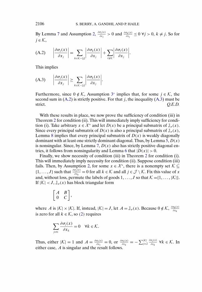
2106 S. BERRY, A. GANDHI, AND P. HAILE

By Lemma 7 and Assumption 2, ∂σj(x)

∂xj> 0 and ∂σk(x)

∂xj≤ 0 ∀j > 0, k �= j. So for

j ∈ K,∣∣∣∣∂σj(x)

∂xj

∣∣∣∣ =∑

k∈K−{j}

∣∣∣∣∂σk(x)

∂xj

∣∣∣∣ +∑�/∈K

∣∣∣∣∂σ�(x)

∂xj

∣∣∣∣�(A.2)

This implies∣∣∣∣∂σj(x)

∂xj

∣∣∣∣ ≥∑

k∈K−{j}

∣∣∣∣∂σk(x)

∂xj

∣∣∣∣�(A.3)

Furthermore, since 0 /∈ K, Assumption 3∗ implies that, for some j ∈ K, thesecond sum in (A.2) is strictly positive. For that j, the inequality (A.3) must bestrict. Q.E.D.

With these results in place, we now prove the sufficiency of condition (iii) inTheorem 2 for condition (ii). This will immediately imply sufficiency for condi-tion (i). Take arbitrary x ∈ X ∗ and let D(x) be a principal submatrix of Jσ(x).Since every principal submatrix of D(x) is also a principal submatrix of Jσ(x),Lemma 8 implies that every principal submatrix of D(x) is weakly diagonallydominant with at least one strictly dominant diagonal. Thus, by Lemma 5, D(x)is nonsingular. Since, by Lemma 7, D(x) also has strictly positive diagonal en-tries, it follows from nonsingularity and Lemma 6 that |D(x)| > 0.

Finally, we show necessity of condition (iii) in Theorem 2 for condition (i).This will immediately imply necessity for condition (ii). Suppose condition (iii)fails. Then, by Assumption 2, for some x ∈ X ∗, there is a nonempty set K ⊆{1� � � � � J} such that ∂σj(x)

∂xk= 0 for all k ∈ K and all j ∈ J \ K. Fix this value of x

and, without loss, permute the labels of goods 1� � � � � J so that K ={1� � � � � |K|}.If |K|< J, Jσ(x) has block triangular form

[A B0 C

]�

where A is |K| × |K|. If, instead, |K| = J, let A = Jσ(x). Because 0 /∈ K, ∂σ0(x)

∂xk

is zero for all k ∈ K, so (2) requires

∑j∈K

∂σj(x)

∂xk

= 0 ∀k ∈ K�

Thus, either |K| = 1 and A = ∂σ1(x)

∂x1= 0, or ∂σ1(x)

∂xk= −∑|K|

j=2∂σj(x)

∂xk∀k ∈ K. In

either case, A is singular and the result follows.

CONNECTED SUBSTITUTES 2107

APPENDIX B: DEMAND FOR DIVISIBLE COMPLEMENTS

Here we demonstrate two assertions made in the discussion of Example 1 inthe text.

PROPOSITION 1: Let q0(p) = q0 be a small positive constant and defineQ(p) = ∑J

j=0 qj(p). Suppose that, for all p such that qj(p) > 0, (i) Q(p) isstrictly decreasing in pj ∀j ≥ 1, and (ii) εjk(p) ≥ εQk(p) ∀k� j �= k. Then As-sumptions 2 and 3 hold for any X ∗ ⊆ X̃ under the transformation σj(p)= qj(p)

Q(p).

PROOF: We first verify the weak substitutes condition. If qj(p) = 0, ∂qj(p)

∂pk

cannot be negative, so the derivative ∂σj(p)

∂pk= ∂qj(p)

∂pk/Q(p) is nonnegative. When

qj(p) > 0, ∂σj(p)

∂pk= [Q(p)

∂qj(p)

∂pk− qj(p)

∂Q(p)

∂pk]/Q(p)2, which is nonnegative if

∂qj(p)

∂pk

pk

qj(p)≥ ∂Q(p)

∂pk

pk

Q(p). We have assumed this in (ii). To show that Assumption 3

holds, observe that since σ0(p) = q0Q(p)

, (i) implies that each good j �= 0 substi-

tutes directly to the artificial good zero on X̃ . Q.E.D.

PROPOSITION 2: For p such that qk(p) ≥ δ > 0 for all k > 0, the hypothe-ses of Proposition 1 hold for q0 sufficiently small when, for all j > 0, qj(p) =Ap−α

j

∏k/∈{0�j} p

−βk with α> β> 0.

PROOF: Part (i) of the hypotheses is immediate since all real goods havedownward sloping demand and are strict gross complements. Since εQk(p) =∑J

j=1 σj(p)εjk(p), part (ii) holds if

−β≥ −[1 − σk(p)− σ0(p)

]β− σk(p)α�

that is,

β≤ qk(p)

qk(p)+ q0α�

Since qk(p)≥ δ > 0 and β< α, this holds for sufficiently small q0. Q.E.D.

APPENDIX C: A LANCASTERIAN EXAMPLE

Consider a simple variation of Lancaster’s (1966) “diet example,” illustrat-ing a continuous demand system with only local substitution, with a non-rectangular domain of interest, and where the introduction of an artificial good0 is useful even though an outside good is already modeled. A representativeconsumer has a budget y and chooses consumption quantities (q1� q2� q3) of

2108 S. BERRY, A. GANDHI, AND P. HAILE

three goods: wine, bread, and cheese, respectively. Her preferences are givenby a utility function

u(q1� q2� q3)= ln(z1)+ ln(z2)+ ln(z3)+m�

where (z1� z2� z3) are consumption of calories, protein, and calcium, and mis money left to spend on other goods. The mapping of goods consumed tocharacteristics consumed is given by18

z1 = q1 + q2 + q3�

z2 = q2 + q3�

z3 = q3�

We assume y > 3. The set of prices (p1�p2�p3) such that all goods are pur-chased is defined by

0 <p1 <p2 −p1 <p3 −p2�(C.1)

Since p plays the role of x here, (C.1) defines X̃ , which is not a rectangle. LetX ∗= X̃ .

It is easily verified that demand for each inside good is given by

σ1(p)= 1p1

− 1p2 −p1

�(C.2)

σ2(p)= 1p2 −p1

− 1p3 −p2

�

σ3(p)= 1p3 −p2

�

for p ∈ X ∗. These equations fully characterize demand for all goods. However,we introduce the artificial quantity of “good 0,” defined by

q0 ≡ 1 −3∑

j=1

qj�(C.3)

Observe that this artificial good is not the outside good m. Further, the con-nected substitutes conditions would not hold if the outside good were treatedas good 0.

18Unlike Lancaster (1966), we sacrifice accuracy of nutritional information for the sake ofsimplicity.

CONNECTED SUBSTITUTES 2109

With (C.2), (C.3) implies

σ0(p)= 1 − 1p1

�

From these equations, it is now easily confirmed that Assumption 2 holds Fur-ther, goods 2 and 3 strictly substitute to each other, goods 1 and 2 strictly substi-tute to each other, and good 1 strictly substitutes to good 0. Thus, Assumption 3also holds.

REFERENCES

AZEVEDO, E., A. WHITE, AND E. G. WEYL (2013): “Walrasian Equilibrium in Large, QuasilinearMarkets,” Theoretical Economics, 8, 281–290. [2097]

BECKERT, W., AND R. BLUNDELL (2008): “Heterogeneity and the Non-Parametric Analysis ofConsumer Choice: Conditions for Invertibility,” Review of Economic Studies, 75, 1069–1080.[2092]

BERRY, S. (1994): “Estimating Discrete Choice Models of Product Differentiation,” RAND Jour-nal of Economics, 23 (2), 242–262. [2091]

BERRY, S., J. LEVINSOHN, AND A. PAKES (1995): “Automobile Prices in Market Equilibrium,”Econometrica, 60 (4), 889–917. [2090-2092,2103]

BERRY, S., O. LINTON, AND A. PAKES (2004): “Limit Theorems for Differentiated Product De-mand Systems,” Review of Economic Studies, 71 (3), 613–614. [2103]

BERRY, S. T., AND P. A. HAILE (2009): “Identification in Differentiated Products Markets UsingMarket Level Data,” Discussion Paper, Yale University. [2087]

(2010a): “Identification in Differentiated Products Markets Using Market Level Data,”Discussion Paper 1744, Cowles Foundation, Yale University. [2092,2103]

(2010b): “Nonparametric Identification of Multinomial Choice Demand Models WithHeterogeneous Consumers,” Discussion Paper 1718, Cowles Foundation at Yale. [2092]

BERRY, S. T., AND A. PAKES (2007): “The Pure Characteristics Demand Model,” Discussion Pa-per, Yale University. [2090,2091]

BERRY, S. T., A. GANDHI AND P. A. HAILE (2011): “Connected Substitutes and Invertibility ofDemand,” Discussion Paper, Yale University. [2094,2095]

BLOCK, H., AND J. MARSCHAK (1960): “Random Orderings and Stochastic Theories of Re-sponses,” in Contributions to Probability and Statistics: Essays in Honor of Harold Hotelling, ed.by I. Olkin, S. Ghurye, W. Hoeffding, W. G. Mado, and H. B. Mann. Stanford, CA: StanfordUniversity Press. [2092]

BRESNAHAN, T. (1981): “Departures From Marginal Cost Pricing in the American AutomobileIndustry,” Journal of Econometrics, 17, 201–227. [2091,2096]

(1987): “Competition and Collusion in the American Automobile Industry: The 1955Price War,” Journal of Industrial Economics, 35, 457–482. [2091]

CHENG, L. (1985): “Inverting Systems of Demand Functions,” Journal of Economic Theory, 37,202–210. [2093]

CHIAPPORI, P.-A., AND I. KOMUNJER (2009): “On the Nonparametric Identification of MultipleChoice Models,” Discussion Paper, University of California San Diego. [2092]

DENECKERE, R., AND M. ROTHSCHILD (1992): “Monopolistic Competition and Preference Di-versity,” Review of Economic Studies, 59, 361–373. [2095]

DIXIT, A., AND J. E. STIGLITZ (1977): “Monopolistic Competition and Optimum Product Diver-sity,” American Economic Review, 67, 297–308. [2097]

DUBE, J.-P. (2004): “Multiple Discreteness and Product Differentiation: Demand for CarbonatedSoft Drinks,” Marketing Science, 23, 66–81. [2095]

2110 S. BERRY, A. GANDHI, AND P. HAILE

DUBE, J.-P., J. FOX, AND C.-L. SU (2012): “Improving the Numerical Performance of BLP Staticand Dynamic Discrete Choice Random Coefficients Demand Estimation,” Econometrica, 80,2231–2267. [2091]

DUBIN, J., AND D. MCFADDEN (1984): “An Econometric Analysis of Residential Electric Appli-ance Holdings and Consumption,” Econometrica, 52 (2), 345–362. [2095]

FALMAGNE, J.-C. (1978): “A Representation Theorem for Finite Random Scale Systems,” Journalof Mathematical Psychology, 18, 52–72. [2092]

GALE, D., AND H. NIKAIDO (1965): “The Jacobian Matrix and Global Univalence of Mappings,”Mathematische Annalen, 159, 81–93. [2089,2090,2092,2093,2100-2102]

GANDHI, A. (2008): “On the Nonparametric Foundations of Discrete Choice Demand Estima-tion,” Discussion Paper, University of Wisconsin–Madison. [2087]

(2010): “Inverting Demand in Product Differentiated Markets,” Discussion Paper, Uni-versity of Wisconsin–Madison. [2091]

GANDHI, A., AND A. NEVO (2011): “Flexible Estimation of Random Coefficient Discrete ChoiceModel Using Aggregate Data,” Discussion Paper, University of Wisconsin. [2091]

GANDHI, A., A. LU, AND X. SHI (2011): “Estimating Discrete Choice Models With Market LevelData: A Bounds Approach,” Discussion Paper, University of Wisconsin–Madison. [2100]

GENTZKOW, M. (2004): “Valuing New Goods in a Model With Complementarity: Online News-papers,” Working Paper, Chicago GSB. [2094]

GOWDA, M. S., AND G. RAVINDRAN (2000): “Algebraic Univalence Theorems for NonsmoothFunctions,” Journal of Mathematical Analysis and Applications, 252, 917–935. [2089]

HADAMARD, J. (1906a): “Sur les Transformations Planes,” Comptes Rendus de la Séances del’Académie Sciences, Paris, 142, 71–84. [2089,2100]

(1906b): “Sur les Transformations Ponctuelles,” Bulletin de la Société Mathématique deFrance, 34, 71–84. [2089,2100]

HANEMANN, W. M. (1984): “Discrete/Continuous Models of Consumer Demand,” Econometrica,52, 541–561. [2095]

HENDEL, I. (1999): “Estimating Multiple-Discrete Choice Models: An Application to Comput-erization Returns,” Review of Economic Studies, 66 (2), 423–446. [2095]

HO, C.-W. (1975): “A Note on Proper Maps,” Proceedings of the American Mathematical Society,51, 237–241. [2102]

HORN, R. A., AND C. R. JOHNSON (1990): Matrix Analysis. Cambridge: Cambridge UniversityPress. [2104]

HOTZ, J., AND R. A. MILLER (1993): “Conditional Choice Probabilites and the Estimation ofDynamic Models,” Review of Economic Studies, 60, 497–529. [2091]

KRANTZ, S. G., AND H. R. PARKS (2002): The Implicit Function Theorem: History, Theory, andApplications. Boston: Birkhäuser. [2102]

LANCASTER, K. J. (1966): “A New Approach to Consumer Theory,” Journal of Political Economy,74, 132–157. [2107,2108]

MAS-COLELL, A. (1979): “Homeomorphisms of Compact, Convex Sets and the Jacobian Matrix,”SIAM Journal of Mathematics, 10, 1105–1109. [2090]

MCFADDEN, D. (1974): “Conditional Logit Analysis of Qualitative Choice Behavior,” in Frontiersof Econometrics, ed. by P. Zarembka. New York: Academic Press. [2091]

(1981): “Econometric Models of Probabilistic Choice,” in Structural Analysis of DiscreteData With Econometric Applications, ed. by C. Manski and D. McFadden. Cambridge, MA:MIT Press. [2091]

(2004): “Revealed Stochastic Preference: A Synthesis,” Discussion Paper, UC Berkeley.[2092]

MCFADDEN, D., AND M. K. RICHTER (1971): “On the Extension of a Set Function on a Set ofEvents to a Probability on the Generated Boolean σ-Algebra,” Discussion Paper, UC Berkeley.[2092]

(1990): “Stochastic Rationality and Revealed Stochastic Preference,” in Preferences,Uncertainty, and Rationality, ed. by J. Chipman, D. McFadden, and M. Richter. Boulder, CO:Westview Press, 161–186. [2092]

CONNECTED SUBSTITUTES 2111

MCKENZIE, L. (1960): “Matrices With Dominant Diagonals and Economic Theory,” in Mathe-matical Methods in the Social Sciences, 1959, ed. by K. Arrow, S. Karlin, and P. Suppes. Stanford:Stanford University Press, 47–62. [2093]

MORÉ, J., AND W. RHEINBOLDT (1973): “On P- and S-Functions and Related Classes of n-Dimensional Nonlinear Mappings,” Linear Algebra and Its Applications, 6, 45–68. [2094]

MOSENSON, R., AND E. DROR (1972): “A Solution to the Qualitative Substitution Problem inDemand Theory,” Review of Economic Studies, 39, 433–441. [2097]

MUSSA, M., AND S. ROSEN (1978): “Monopoly and Product Quality,” Journal of Economics The-ory, 18, 301–307. [2090,2096]

NOVSHEK, W., AND H. SONNENSCHEIN (1979): “Marginal Consumers and Neoclassical DemandTheory,” Journal of Political Economy, 87, 1368–1376. [2095]

PALAIS, R. S. (1959): “Natural Operations on Differential Forms,” Transactions of the AmericanMathematical Society, 92, 125–141. [2090,2092,2102]

PARTHASARATHY, T. (1983): On Global Univalence Theorems. Berlin: Springer. [2089,2102]PARTHASARATHY, T., AND G. RAVINDRAN (2003): “Global Univalence and the Jacobian Con-

jecture,” in Applicable Mathematics in the Golden Age, ed. by J. Misra. New Delhi: NarosaPublishing House. [2089,2102]

PERLOFF, J. M., AND S. C. SALOP (1985): “Equilibrium With Product Differentiation,” Review ofEconomic Studies, 52, 107–120. [2095]

RADULESCU, M., AND S. RADULESCU (1980): “GLobal INversion Theorems and Applictionsto Diffeerential Equations,” Nonlinear Analysis Theory. Methods and Applications, 4, 951–965.[2090]

RHEINBOLDT, W. C. (1970a): “On Classes of n-Dimensional Nonlinear Mappings GeneralizingSeveral Types of Matrices,” Discussion Paper, University of Maryland. [2103]

(1970b): “On M-Functions and Their Application to Nonlinear Gauss–Seidel Iterationsand to Network Flows,” Journal of Mathematical Analysis and Applications, 32, 274–307. [2100]

ROCHET, J.-C., AND L. A. STOLE (2002): “Nonlinear Pricing With Random Participation,” Reviewof Economic Studies, 69 (1), 277–311. [2096]

SALOP, S. (1979): “Monopolistic Competition With Outside Goods,” RAND Journal of Economics,10, 141–156. [2090,2096]

SOUZA-RODRIGUES, E. (2011): “Nonparametric Estimator of a Generalized Regression ModelWith Group Effects,” Working Paper, Yale University. [2091]

SPENCE, M. (1976): “Product Selection, Fixed Costs and Monopolistic Competition,” Review ofEconomic Studies, 43, 217–236. [2095,2097]

TAUSSKY, O. (1949): “A Recurring Theorem on Determinants,” The American MathematicalMonthly, 56 (10), 672–676. [2104,2105]

Dept. of Economics, Yale University, 37 Hillhouse Avenue, New Haven, CT06520, U.S.A., and NBER and Cowles Foundation; steven.berry@yale.edu,

Dept. of Economics, University of Wisconsin, 1180 Observatory Drive, Madison,WI 53706, U.S.A.; agandhi@ssc.wisc.edu,

andDept. of Economics, Yale University, 37 Hillhouse Avenue, New Haven, CT

06520, U.S.A., and NBER and Cowles Foundation; philip.haile@yale.edu.

Manuscript received June, 2011; final revision received March, 2013.