Conjugate Rotation: Parameterization and Estimationfrom an Affine Feature Correspondence

Kevin Koser, Christian Beder and Reinhard KochChristian-Albrechts-University

Kiel, Germany{koeser,beder,rk}@mip.informatik.uni-kiel.de

Abstract

When rotating a pinhole camera, images are related bythe infinite homography KRK−1, which is algebraicallya conjugate rotation. Although being a very common im-age transformation, e.g. important for self-calibration orpanoramic image mosaicing, it is not completely under-stood yet. We show that a conjugate rotation has 7 degreesof freedom (as opposed to 8 for a general homography) andgive a minimal parameterization. To estimate the conju-gate rotation, authors traditionally made use of point cor-respondences, which can be seen as local zero order Tay-lor approximations to the image transformation. Recentlyhowever, affine feature correspondences have become in-creasingly popular. We observe that each such affine corre-spondence now provides a local first order Taylor approx-imation, which has not been exploited in the context of ge-ometry estimation before. Using those two novel conceptsabove, we finally show that it is possible to estimate a con-jugate rotation from a single affine feature correspondenceunder the assumption of square pixels and zero skew. As abyproduct, the proposed algorithm directly yields rotation,focal length and principal point.

1. Introduction

The infinite homography H∞ = K1RK−12 is an image-

to-image transformation, which relates points in one im-age with points in another image, if the camera has eitheronly rotated or the corresponding 3D point is infinitely faraway. It is a very important concept in self-calibration [22],projective geometry [9], or when dealing with purely ro-tating cameras, e.g. with pan-tilt-units [4], or for creatingpanoramic image mosaics[3].

In this work we concentrate on the case of constant in-trinsic camera parameters, i.e. we assume K1 = K2. Then,algebraically a 3x3-matrix H acting in the projective imagespace P2 is such an infinite homography, if and only if it is

proportional to a conjugate rotation, i.e. has the same eigen-value structure as a scaled rotation matrix [9].

However, the dimension and structure of the set of conju-gate rotations within the space of all possible homographieshas not been fully understood yet, so that no algorithm forthe direct computation of general conjugate rotations cur-rently exists. So far a solution exists only for the specialcase when nearly all intrinsics (skew, aspect ratio, princi-pal point) are known exactly [2]. In the general case, re-searchers typically estimate general homographies (e.g. us-ing direct linear transformation [9] on n ≥ 4 point corre-spondences) and state that - in the presence of little noise -the estimate should not be too far from a conjugate rotation[10, 4]. However, even in this case enforcing the “conjugaterotation constraints” afterwards is not as straightforward asfor instance in the 8-point algorithm [9] for the fundamentalmatrix, because the eigenvalue decomposition of H∞ willin general contain complex vectors. Simply projecting ontothe allowed manifold has not been possible, because nei-ther the dimension of this manifold has been known nor asuitable minimal parameterization is available.

In this work we will propose such a minimal parame-terization for the conjugate rotation and show that the setof conjugate rotations is a 7-dimensional manifold in thespace of all 3x3-matrices R9. As a second contribution wewill show how to estimate a conjugate rotation from a sin-gle affine feature (cf. to [19]) correspondence, which pro-vides already 6 constraints, using the additional assumptionof zero skew and square pixels. This is in contrast to the al-gorithm presented in [2], which also requires the principalpoint to be known exactly, which is not always available.

This work is structured as follows: since the proposedparameterization and estimation is based upon a novel dif-ferential constraint from affine feature correspondences, wewill start by explaining the concept of such a correspon-dence (a first order Taylor approximation of H∞) in section2 before we come to the conjugate rotation in section 3. Insection 4, we will present a direct way of computing theconjugate rotation from a single affine correspondence and

1

either another point or line correspondence or using the as-sumption of zero skew and square pixels. In the latter caserotation, focal length and principal point of the camera di-rectly result from the proposed algorithm. Finally, in sec-tion 5 we will evaluate our novel algorithm, investigate itssensitivity to disturbances of the affine correspondence andshow results in panoramic mosaicing with real images.

Notation: To improve the readability of the equationswe use the following notation in this paper. Boldface italicserif letters x denote Euclidean vectors while boldface up-right serif letters x denote homogeneous vectors. For ma-trices we do not use serifs, so that Euclidean matrices aredenoted as A and homogeneous matrices are denoted as A.

2. Affine CorrespondencesProgress in robust local features (cf. to [19, 18] for a

thorough discussion) allows automatic matching of imagesin which appearance of local regions undergoes approxi-mately affine changes of brightness and/or of shape, e.g.for automated panorama generation[3] or scene reconstruc-tion through wide-baseline matching[24]. The idea is thatinteresting features are detected in each image and that thesurrounding region of each feature is normalized with re-spect to the local image structure in this region, leading toabout the same normalized regions for correspondences indifferent images, which can be exploited for matching. Theconcatenation of the normalizations provides affine corre-spondences between different views, i.e. not only a point-to-point relation but also a relative transformation of the lo-cal region (imagine scale, shear or rotation).

Although such correspondences carry more informationthan the traditional point correspondence used in estima-tion of multiple view geometry [9], this additional informa-tion is rarely used. Approaches not using point correspon-dences deal with conic correspondences [12, 11], whichtypically lead to systems of quadratic equations or requirelots of matrix factorizations. Others require the identifi-cation of locally planar rectangle correspondences [13] forH∞-computation. Schmid and Zisserman[25] investigatedthe behavior of local curvature under homography mapping.Chum et al. noted in [5] that an affine correspondence issomehow equivalent to three point correspondences: in ad-dition to the center point two further points can be detectedin the feature coordinate system (the local affine frame).This allowed the estimation of a fundamental matrix from3 affine feature correspondences (from which 9 point cor-respondence were generated). The “local sampling” of theaffine feature concept was recently also adopted by Riggi etal. [23] for fundamental matrix estimation and by Perdochet al. for extended essential matrix estimation[20].

In contrast to the latter we do not sample but use a com-pact analytic expression for the whole correspondence: Weobserve that the concatenation of the normalization trans-

Figure 1. An affine correspondence in two images related by aninfinite homography H∞: The linear transformation (e.g. shear,rotation, magnification) between the two magnified image regionsapproximates the local derivative of the global image-to-imagemapping H∞ in the center of the window. Considering also thecenter shift, the resulting affine transformation can be thought ofbeing tangent to H∞, which can be exploited for estimation.

formations provides a good approximation to the first or-der Taylor expansion of the homography, i.e. that the affinetransform is the linearization of the homography (see alsofigure 1):

H(x) = H(x0) +∂H(x)∂x

∣∣∣∣x0

(x− x0) + . . . (1)

A ≈ ∂H(x)∂x

∣∣∣∣x0

A ∈ R2×2 (2)

Here H : R2 → R2 is the homography mapping betweenthe two images in Euclidean coordinates and A representslocal shear, scale and rotation between the two correspond-ing features.

This is actually already exploited for matching but hasnot been used for geometry estimation before. As will beseen in the next section, using this compact representationof a correspondence keeps local relations and allows for pa-rameterizing the conjugate rotation, because it provides adifferential constraint on the local image transformation.

2.1. Upgrade and Refinement

The considerations so far apply to affine covariant fea-tures (e.g. MSER[16]). However, if matches result fromweaker features (e.g. DoG/SIFT[14]), the proposed methodcan also be applied. The main insight is that if a correctmatch has been established such that the local regions areapproximately aligned, the affine transform based upon therelative parameters is already almost correct. The straight-forward way is to compute the affine transformation directlyfrom the local frames of these features. This is usually al-ready quite close to correct, because the correct match is aresult from a high image similarity, e.g. in small baselinematching. However, since we need an accurate estimate ofthe Jacobian of the image transformation, it is reasonableeven for already affine features to apply a gradient-based

optimization of A using the Lucas-Kanade approach [15, 1].The concept of A as the local derivative of the image trans-form now leads to a parameterization of the conjugate rota-tion, as is shown in the next section.

3. The Infinite Homography: A Conjugate Ro-tation

We will now derive a minimal parameterization for theconjugate rotation. Despite being a very important conceptin multi view geometry, the number of degrees of freedomhas not been investigated yet. Neither exists a parameteri-zation with less than the 8 parameters (as the naive param-eterization with 5 intrinsic parameters and 3 rotation pa-rameters). Such an over-parameterization can cause trou-ble in optimization, e.g. degenerate covariance matrices inmaximum-likelihood estimation. Some authors have sim-plified K for the conjugate rotation to pure diagonal shapewith zero skew, known aspect ratio and principal point [2].Consequently, in this simplified model only a subset of allpossible conjugate rotations is allowed. Instead, we willnow derive a minimal parameterization for general conju-gate rotations and will then discuss estimation in the nextsection. A 2d homography mapping

x′ ' Hx =

hT1

hT2

d

hT3 1

x (3)

is expressed in Euclidean coordinates as

x′ =

(hT

1

hT2

)x+ d

hT3x+ 1

(4)

Its derivative is

A =(a11 a12

a21 a22

)=∂x′

∂x= (5)

(hT3x+ 1)

(hT

1

hT2

)−(hT

1

hT2

)xhT

3 − dhT3

(hT3x+ 1)2

We now change without loss of generality the coordinatesystems of both images, such that x = (0, 0)T, then thissimplifies to

A =(hT

1

hT2

)− dhT

3 (6)

Solving this for h3 and using d = x′ − x, the homogra-phy given x′ and A is therefore

H =(

A + (x′ − x)hT3 x′ − x

hT3 1

)(7)

=(

I2 x′ − x0T

2 1

)(A 02

hT3 1

)(8)

So far, H may be any homography and no special con-jugate rotation assumptions have been made. We will nowassume that H is proportional to a conjugate rotation, i.e.

H = λKRK−1 (9)

where R is the relative camera rotation and K is the cam-era calibration matrix holding focal length f , aspect ratio a,skew s and principal point (cx, cy)T:

K =

f s cx0 a f cy0 0 1

(10)

From the orthogonality of the rotation matrix R followsthat its eigenvalues and therefore also the eigenvalues of 1

λHare {1, eiφ, e−iφ}. Exploiting that all eigenvalues have thesame absolute value, Pollefeys et al. derived a fourth orderpolynomial constraint for self-calibration, called the mod-ulus constraint [21], which is a neccessary condition for aconjugate rotation. In contrast to this the above parame-terization now leads to a linear relation between h31 andh32, which provides a sufficient condition for conjugate ro-tations. We therefore factorize its characteristic polynomialinto its roots

det(

1λ

H− τ I3

)= α(τ − 1)(τ − eiφ)(τ − e−iφ) (11)

Multiplying out both sides yields a 3rd order polynomial inτ on both sides of the equation.

c3τ3 + c2τ

2 + c1τ + c0 = (12)

ατ3 − α(eiφ + e−iφ + 1)τ2 + α(eiφ + e−iφ + 1)τ − αwhere the coefficients ci depend on H and λ. By compar-ison of the polynomial coefficients we eliminate the un-knowns α and φ and obtain two constraints, which areequivalent to

λ3 = det A (13)

λtr(H) =12((tr(H))2 − tr(H2)) (14)

Observe that eq. (13) eliminates the scale factor λ from sub-sequent computations and that all homographies, which ful-fill these constraints, must be conjugate rotations. We nowinsert equation (7) into those constraints and obtain the con-dition (

(λ− trA)(x′ − x)T + (x′ − x)TAT)h3 (15)

=12(trA)2 − trA− 1

2tr(

A2)− λ (trA + 1)

which is linear in h3, so that, given an affine feature corre-spondence (x ↔ x′, A), only one unknown h32 is left, i.e.we can write

h3 =(ah32 + bh32

)(16)

for some a and b derived from the linear constraint of equa-tion (15). From a geometrical point of view the equationabove enforces the fixpoint of the conjugate rotation: thefixpoint is the eigenvector corresponding to the eigenvalue1 (the intersection of the rotation axis and the image plane).

We now have a family of homographies, which dependson the six parameters of the affine correspondence and oneparameter of the equation above. In other words, the nine-dimensional H depends on seven parameters

p = (a11, a12, a21, a21, d1, d2, h32)T (17)

now. By construction, H must be a conjugate rotation andthe manifold for conjugate rotation can have at most sevendimensions, since it depends on seven parameters only. Weevaluate the Jacobian ∂H/∂p, which is a 9 by 7 matrix withthe partial derivatives of the 9 entries of H. Proving linearindependence of seven of the columns is quite tedious andlengthy, but using a symbolic linear algebra processor[17]we obtained that

rank(∂H/∂p) = 7 (18)

Intuitively this means, that if we vary p we can run in 7orthogonal directions on the manifold and this defines thedimension of the manifold [8].

This may be surprising at first sight, since knowing theeigenvalue structure seems to be more information than asingle constraint[21]. Note however, that the rotation an-gle φ is unknown and we therefore only know the absolutevalue of the second and the third eigenvalue. Also, sincethe characteristic polynomial is holomorphic (as all polyno-mials), complex conjugates of any root must also be a rootand finally, in projective space a homography is equivalentto a scaled version, so we basically end up with the con-straint “All eigenvalues have the same absolute value”. Inthe next section we show how the conjugate rotation with its7 degrees of freedom can be estimated based upon an affinecorrespondence, which already provides 6 constraints.

4. Estimation and Self-Calibration with Con-straints

In the previous section we derived a homography of theform

H(h32) =(

I2 x′ − x0T

2 1

)(A 02

hT3 1

)(19)

which, given an affine feature correspondence, dependsonly on one parameter h32. Basically this means that theaffine transform locally fixes the conjugate rotation, but thepre-image of the line at infinity h3 still depends on one un-known parameter: we do not know, what maps to infinityyet.

In order to determine this remaining parameter we needone additional constraint. This may be obtained from an-other point or line correspondence or from a constraint onthe intrinsic camera parameters.

4.1. Additional Point or Line Correspondence

If an additional image point correspondence (y,y′) isgiven, it must fulfill the homography mapping (using theparameterization from equation (19))(

y′ − x1

)' H

(y − x

1

)(20)

=(

I2 x′ − x0T

2 1

)(A 02

hT3 1

)(y − x

1

)We bring the displacement matrix to the left hand side

and require that the cross product of the left hand side andthe right hand side is zero[

y′ − x′1

]×

(02×2

(y − x)T

)h3 (21)

= −[y′ − x′

1

]×

(A(y − x)

1

)Selecting one of the first two rows yields a linear equa-

tion in h3, which in general1 determines the last remain-ing degree of freedom and therefore the conjugate rotationwithout any restrictions on skew, aspect ratio, focal lengthor principal point. Alternatively, another line correspon-dence might be used, e.g. if the horizon can be found inboth images. Lines are dual to points and backward-mapwith a transposed H, so basically the same linear algebraapplies as in the point correspondence case.

Self calibration is now possible with the approach ofHartley [10]. Note however, that in contrast to the homogra-phy estimation method used in [10], our estimated homog-raphy will be a perfect conjugate rotation.

If on the other hand some intrinsics of the used cameraare known beforehand, no additional correspondence is re-quired for estimation of the infinite homography as will beshown next.

4.2. Constraints on the Intrinsics

If only a single affine feature correspondence is given,the remaining unknown h32 may be computed using con-straints on the intrinsic camera parameters. We will assumezero skew and unit aspect ratio in the following, which istrue for most consumer cameras on the market. The onlyother algorithm to estimate a conjugate rotation [2] addi-tionally requires the exact principal point position (see fig-ure 2 for the sensitivity of [2] to principal point deviations).

1In the case that the point is on the line between the fixpoint and theaffine feature, equations (16) and (21) will not be linearly independent. Inthis case a different point must be used.

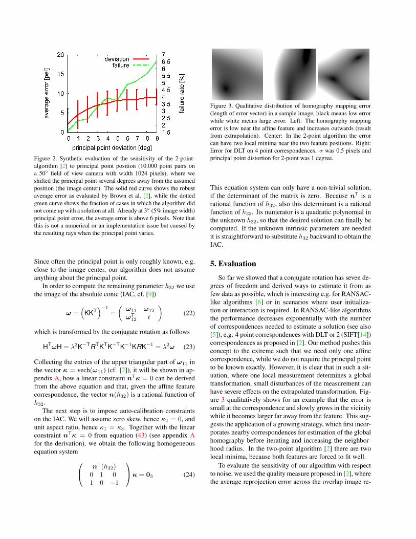
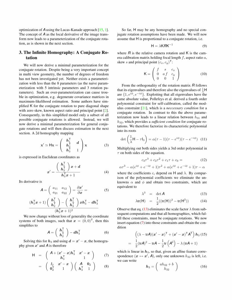
Figure 2. Synthetic evaluation of the sensitivity of the 2-point-algorithm [2] to principal point position (10.000 point pairs ona 50◦ field of view camera with width 1024 pixels), where weshifted the principal point several degrees away from the assumedposition (the image center). The solid red curve shows the robustaverage error as evaluated by Brown et al. [2], while the dottedgreen curve shows the fraction of cases in which the algorithm didnot come up with a solution at all. Already at 3◦ (5% image width)principal point error, the average error is above 6 pixels. Note thatthis is not a numerical or an implementation issue but caused bythe resulting rays when the principal point varies.

Since often the principal point is only roughly known, e.g.close to the image center, our algorithm does not assumeanything about the principal point.

In order to compute the remaining parameter h32 we usethe image of the absolute conic (IAC, cf. [9])

ω =(

KKT)−1

=(ω11 ω12

ωT12 t

)(22)

which is transformed by the conjugate rotation as follows

HTωH = λ2K−TRTKTK−TK−1KRK−1 = λ2ω (23)

Collecting the entries of the upper triangular part of ω11 inthe vector κ = vech(ω11) (cf. [7]), it will be shown in ap-pendix A, how a linear constraint nTκ = 0 can be derivedfrom the above equation and that, given the affine featurecorrespondence, the vector n(h32) is a rational function ofh32.

The next step is to impose auto-calibration constraintson the IAC. We will assume zero skew, hence κ2 = 0, andunit aspect ratio, hence κ1 = κ3. Together with the linearconstraint nTκ = 0 from equation (43) (see appendix Afor the derivation), we obtain the following homogeneousequation system nT(h32)

0 1 01 0 −1

κ = 03 (24)

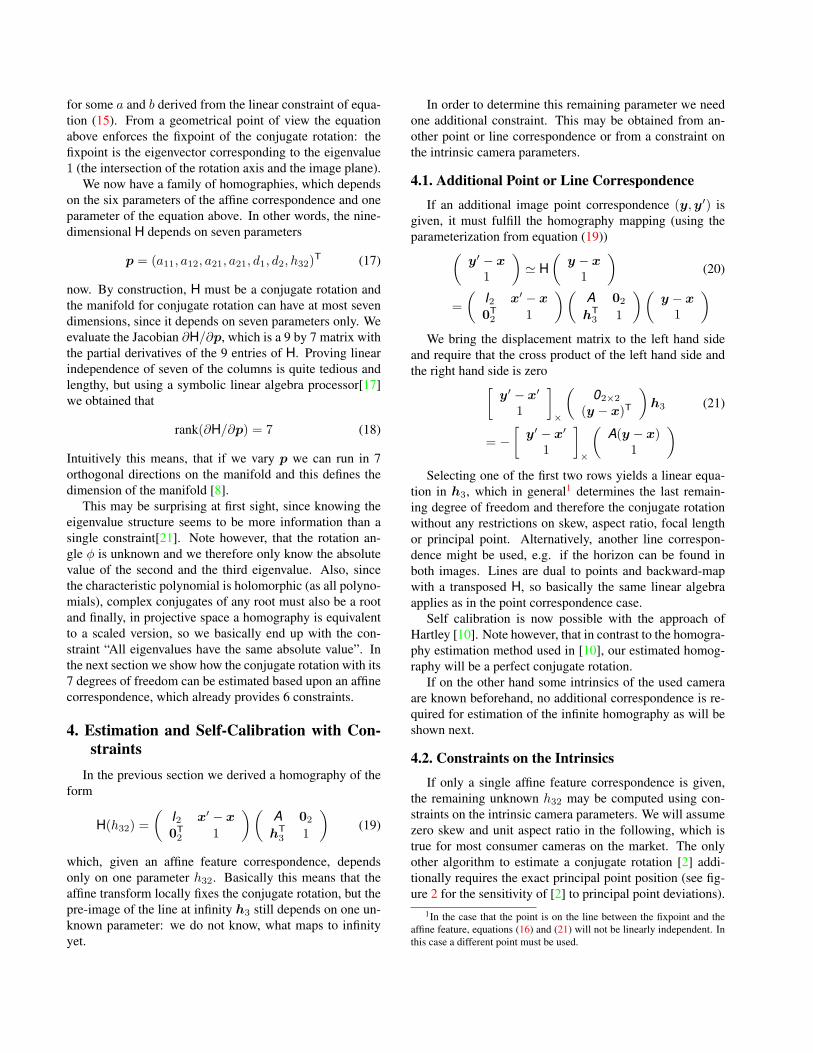
Figure 3. Qualitative distribution of homography mapping error(length of error vector) in a sample image, black means low errorwhile white means large error. Left: The homography mappingerror is low near the affine feature and increases outwards (resultfrom extrapolation). Center: In the 2-point algorithm the errorcan have two local minima near the two feature positions. Right:Error for DLT on 4 point correspondences. σ was 0.5 pixels andprincipal point distortion for 2-point was 1 degree.

This equation system can only have a non-trivial solution,if the determinant of the matrix is zero. Because nT is arational function of h32, also this determinant is a rationalfunction of h32. Its numerator is a quadratic polynomial inthe unknown h32, so that the desired solution can finally becomputed. If the unknown intrinsic parameters are neededit is straightforward to substitute h32 backward to obtain theIAC.

5. Evaluation

So far we showed that a conjugate rotation has seven de-grees of freedom and derived ways to estimate it from asfew data as possible, which is interesting e.g. for RANSAC-like algorithms [6] or in scenarios where user initializa-tion or interaction is required. In RANSAC-like algorithmsthe performance decreases exponentially with the numberof correspondences needed to estimate a solution (see also[5]), e.g. 4 point correspondences with DLT or 2 (SIFT[14])correspondences as proposed in [2]. Our method pushes thisconcept to the extreme such that we need only one affinecorrespondence, while we do not require the principal pointto be known exactly. However, it is clear that in such a sit-uation, where one local measurement determines a globaltransformation, small disturbances of the measurement canhave severe effects on the extrapolated transformation. Fig-ure 3 qualitatively shows for an example that the error issmall at the correspondence and slowly grows in the vicinitywhile it becomes larger far away from the feature. This sug-gests the application of a growing strategy, which first incor-porates nearby correspondences for estimation of the globalhomography before iterating and increasing the neighbor-hood radius. In the two-point algorithm [2] there are twolocal minima, because both features are forced to fit well.

To evaluate the sensitivity of our algorithm with respectto noise, we used the quality measure proposed in [2], wherethe average reprojection error across the overlap image re-

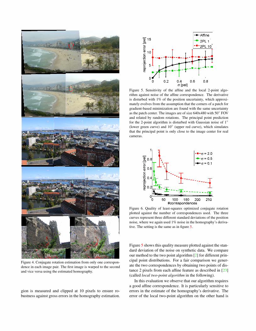
Figure 4. Conjugate rotation estimation from only one correspon-dence in each image pair. The first image is warped to the secondand vice versa using the estimated homography.

gion is measured and clipped at 10 pixels to ensure ro-bustness against gross errors in the homography estimation.

Figure 5. Sensitivity of the affine and the local 2-point algo-rithm against noise of the affine correspondence. The derivativeis disturbed with 1% of the position uncertainty, which approxi-mately evolves from the assumption that the corners of a patch forgradient-based minimization are found with the same uncertaintyas the patch center. The images are of size 640x480 with 50◦ FOVand related by random rotations. The principal point predictionfor the 2-point algorithm is disturbed with Gaussian noise of 1◦

(lower green curve) and 10◦ (upper red curve), which simulatesthat the principal point is only close to the image center for realcameras.

Figure 6. Quality of least-squares optimized conjugate rotationplotted against the number of correspondences used. The threecurves represent three different standard deviations of the positionnoise, where we again used 1% noise in the homography’s deriva-tive. The setting is the same as in figure 5.

Figure 5 shows this quality measure plotted against the stan-dard deviation of the noise on synthetic data. We compareour method to the two point algorithm [2] for different prin-cipal point distributions. For a fair comparison we gener-ate the two correspondences by obtaining two points of dis-tance 2 pixels from each affine feature as described in [23](called local two-point algorithm in the following).

In this evaluation we observe that our algorithm requiresa good affine correspondence. It is particularly sensitive toerrors in the estimate of the homography’s derivative. Theerror of the local two-point algorithm on the other hand is

dominated by the principal point distortion. However, ifmany correspondences are available the novel minimal pa-rameterization allows for a simple nonlinear least squaresmaximum likelihood optimization of conjugate rotationsgiven affine feature correspondences. Figure 6 shows thereprojection error plotted against the number of correspon-dences for different noise levels. The reprojection error de-creases significantly if more affine feature correspondencesare used.

Next we obtained SIFT-feature correspondences be-tween the images pairs depicted in figure 4 according to themethod of [3] and computed focal length and principal pointfrom each of the correspondences, which we refined before-hand to enhance the accuracy of the homography’s deriva-tive estimate. While some of the estimates were reasonable,we observe that the variation in the resulting intrinsic pa-rameters was too large, so that the one-feature approach forauto-calibration seems rather of theoretical interest.

Finally, we demonstrate some results on real imagestaken with different cameras as depicted in figure 4. Fromonly one local correspondence we estimated a conjugate ro-tation using the proposed algorithm under the assumptionof zero skew and square pixels. The images were stitchedtogether and the results are shown in figure 4. Althoughnot being subpixel correct, particularly in regions far awayfrom the correspondence, we find the results quite appealinggiven the minimalistic data they are based upon.

6. ConclusionWe have shown that a general conjugate rotation has

seven degrees of freedom and proposed a minimal parame-terization. This parameterization arises from the insight thatan affine feature correspondence provides a first order Tay-lor approximation to the image transformation, allowing fora differential constraint onto the homography.

The second major contribution of this work is an algo-rithm for estimating a conjugate rotation from a single affinefeature correspondence under the assumption of zero skewand known aspect ratio involving nothing more expensivethan the solution of a quadratic equation.

Also, our method does not require the principal pointto be exactly at the image center, a crucial assumption towhich previous methods are sensitive to, but which mightnot exactly be fulfilled in real cameras. Although not be-ing suitable for auto-calibration, we have demonstrated thatpanoramic stitching is possible using only one single affinefeature correspondence.

A. Constraints on the IACWe will now show, how to derive a linear constraint

nTκ = 0 on κ = vech(ω11) (cf. equation (22) and [7])from equation (23). Therefore we first compute the left

hand side of equation (23) stepwise. Starting with the in-ner part, the translated conic is(

I2 02

(x′ − x)T 1

)(ω11 ω12

ωT12 t

)(I2 x′ − x0T

2 1

)=(ω11 φ12

φT12 u

)(25)

with the substitution

φ12 = ω12 + ω11(x′ − x) (26)

u = t− (x′ − x)Tω11(x′ − x) + 2φT12(x

′ − x) (27)

Next we apply the affine and projective part of the trans-formation yielding(

AT h3

0T2 1

)(ω11 φ12

φT12 u

)(A 02

hT3 1

)=(ρ11 ρ12

ρT12 u

)(28)

with the substitutions

ρ11 = ATω11A + h3φT12A + ATφ12h

T3 + h3uh

T3 (29)

ρ12 = ATφ12 + h3u (30)

From equation (23) now follows u = λ2t, ρ12 = λ2ω12

and ρ11 = λ2ω11. We start by substituting u = λ2t intoequation (27) yielding

u =λ2

1− λ2((x′−x)Tω11(x′−x)−2φT

12(x′−x)) (31)

Next we solve equation (26) for ω12 and obtain from thecondition ρ12 = λ2ω12 and equation (30) the equation

ATφ12 + h3u = λ2(φ12 − ω11(x′ − x)) (32)

Substituting equation (31) and solving this for φ12 yields

φ12 = Mκ (33)

withM = P−1Q((x′ − x)T ⊗ I2)D2 (34)

using the substitutions

P = λ2

(I2 +

21− λ2

h3(x′ − x)T)− AT (35)

Q = λ2

(I2 +

11− λ2

h3(x′ − x)T)

(36)

and the duplication matrix

D2 =

1 0 00 1 00 1 00 0 1

(37)

Substituting this back into equation (31) yields

u = mTκ (38)

with

mT =λ2

1− λ2(x′−x)T(I2− 2P−1Q)((x′−x)T⊗ I2)D2

(39)Finally we use the last remaining condition ρ11 =

λ2ω11 and obtain from equation (29) the condition

ATω11A + h3φT12A + ATφ12h

T3 + h3uh

T3 − λ2ω11 = 02

(40)Substituting equations (33) and (38) yields the homoge-neous linear equation system

Nκ = 04 (41)

with

N = (AT ⊗ AT)D2 + (ATM)⊗ h3 (42)

+h3 ⊗ (ATM) + h3 ⊗ (h3mT)− λ2D2

This equation system contains only rational functions of h32

(the denominator is det P, as P−1 = P∗/ det P) and turnsout to have only rank 1. Hence we may select one singlerow nT from N

nTκ = 0 (43)

which is the desired result.

Acknowledgments

This work has been supported by the German ResearchFoundation (DFG) in the project KO-2044/3-1.

References[1] S. Baker and I. Matthews. Lucas-Kanade 20 Years On: A

Unifying Framework. International Journal of Computer Vi-sion, 56(3):221–255, 2004. 3

[2] M. Brown, R. Hartley, and D. Nister. Minimal solutions forpanoramic stitching. In Proceedings of CVPR 2007, 2007. 1,3, 4, 5, 6

[3] M. Brown and D. G. Lowe. Automatic panoramic imagestitching using invariant features. International Journal ofComputer Vision, 74(1):59–73, 2007. 1, 2, 7

[4] D. Capel and A. Zisserman. Automatic mosaicing withsuper-resolution zoom. In Proceedings of CVPR 1998, page885, Washington, DC, USA, 1998. IEEE Computer Society.1

[5] O. Chum, J. Matas, and S. Obdrzalek. Epipolar geometryfrom three correspondences. In Proc. Computer Vision Win-ter Workshop 2003, Prague, pages 83–88, 2003. 2, 5

[6] M. Fischler and R. Bolles. RANdom SAmpling Consensus:a paradigm for model fitting with application to image analy-sis and automated cartography. Communications of the ACM,24(6):381–395, 1981. 5

[7] A. Fusiello. A matter of notation: Several uses of the kro-necker product in 3d computer vision. Pattern RecognitionLetters, 28:2127–2132, 2007. 5, 7

[8] A. Gray. Modern Differential Geometry of Curves and Sur-faces. CRC Press, Boca Raton, Florida, 1994. 4

[9] R. Hartley and A. Zissermann. Multiple View Geometry inComputer Vision. Cambridge university press, second edi-tion, 2004. 1, 2, 5

[10] R. I. Hartley. Self-calibration from multiple views with arotating camera. In LNCS 800 (ECCV 94), pages 471–478.Springer-Verlag, 1994. 1, 4

[11] F. Kahl and A. Heyden. Using conic correspondence in twoimages to estimate the epipolar geometry. In Proceedings ofICCV, pages 761–766, 1998. 2

[12] Kannala, Salo, and Heikkila. Algorithms for computing aplanar homography from conics in correspondence. In Pro-ceedings of BMVC 2006, 2006. 2

[13] J.-S. Kim and I. S. Kweon. Infinite homography estima-tion using two arbitrary planar rectangles. In Proceedingsof ACCV 2006, pages 1–10, 2006. 2

[14] D. G. Lowe. Distinctive Image Features from Scale-Invariant Keypoints. International Journal of Computer Vi-sion, 60(2):91–110, 2004. 2, 5

[15] B. Lucas and T. Kanade. An Iterative Image RegistrationTechnique with an Application to Stereo Vision. In IJCAI81,pages 674–679, 1981. 3

[16] J. Matas, O. Chum, M. Urban, and T. Pajdla. Robust Widebaseline Stereo from Maximally Stable Extremal Regions. InProceedings of BMVC02, 2002. 2

[17] Matlab Symbolic Math Toolbox V.3.2(R2007a). 4[18] K. Mikolajczyk and C. Schmid. A Performance Evaluation

of local Descriptors. IEEE Transactions Pattern Analysisand Machine Intelligence, 27(10):1615–1630, 2005. 2

[19] K. Mikolajczyk, T. Tuytelaars, C. Schmid, A. Zisserman,J. Matas, F. Schaffalitzky, T. Kadir, and L. Van Gool. AComparison of Affine Region Detectors. International Jour-nal of Computer Vision, 65(1-2):43–72, 2005. 1, 2

[20] M. Perdoch, J. Matas, and O. Chum. Epipolar geometry fromtwo correspondences. In Proceedings of ICPR 2006, pages215–220, 2006. 2

[21] M. Pollefeys and L. V. Gool. Stratified self-calibration withthe modulus constraint. IEEE Transactions on Pattern Anal-ysis and Machine Intelligence, 21(8):707–724, 1999. 3, 4

[22] R.Hartley. Self-calibration of stationary cameras. Interna-tional Journal of Computer Vision, 22(1):5–23, 1997. 1

[23] F. Riggi, M. Toews, and T. Arbel. Fundamental matrix esti-mation via TIP - transfer of invariant parameters. In Proceed-ings of the 18th International Conference on Pattern Recog-nition, pages 21–24, Hong Kong, August 2006. 2, 6

[24] F. Rothganger, S. Lazebnik, C. Schmid, and J. Ponce. 3dobject modeling and recognition using local affine-invariantimage descriptors and multi-view spatial constraints. Int. J.Comput. Vision, 66(3):231–259, 2006. 2

[25] C. Schmid and A. Zisserman. The geometry and matching oflines and curves over multiple views. International Journalof Computer Vision, 40(3):199–234, 2000. 2