Embed Size (px)
Citation preview

Bayesian Analysis (0000) 00 Number 0 pp 1
Conjugate Priors and Posterior Inference forthe Matrix Langevin Distribution on the Stiefel
Manifold
Subhadip Pallowast Subhajit Senguptadagger Riten Mitralowast and Arunava BanerjeeDagger
Abstract
Directional data emerges in a wide array of applications ranging from atmo-spheric sciences to medical imaging Modeling such data however poses uniquechallenges by virtue of their being constrained to non-Euclidean spaces like man-ifolds Here we present a unified Bayesian framework for inference on the Stiefelmanifold using the Matrix Langevin distribution Specifically we propose a novelfamily of conjugate priors and establish a number of theoretical properties rel-evant to statistical inference Conjugacy enables translation of these propertiesto their corresponding posteriors which we exploit to develop the posterior in-ference scheme For the implementation of the posterior computation includingthe posterior sampling we adopt a novel computational procedure for evaluatingthe hypergeometric function of matrix arguments that appears as normalizationconstants in the relevant densities
Keywords Bayesian Inference Conjugate Prior Hypergeometric Function ofMatrix Argument Matrix Langevin Distribution Stiefel ManifoldVectorcardiography
Department of Bioinformatics and Biostatistics University of Louisvillelowast
Center for Psychiatric Genetics NorthShore University HealthSystemdagger
Department of Computer amp Information Science amp Engineering University of FloridaDagger
ccopy 0000 International Society for Bayesian Analysis DOI 0000
imsart-ba ver 20141016 file BA1176_papertex date August 11 2019
2
1 Introduction
Analysis of directional data is a major area of investigation in statistics Directionaldata range from unit vectors in the simplest case to sets of ordered orthonormal framesin the general scenario Since the associated sample space is non-Euclidean standardstatistical methods developed for the Euclidean space may not be appropriate to an-alyze such data Additionally it is often desirable to design statistical methods thattake into consideration the underlying geometric structure of the sample space Thereis a need for methodological development for a general sample space such as the Stiefelmanifold (James 1976 Chikuse 2012) that goes beyond those techniques designed forsimpler non-Euclidean spaces like the circle or the sphere Such a novel methodology cansupport various emerging applications increasingly seen in the fields of biology (Downs1972 Mardia and Khatri 1977) computer science (Turaga et al 2008 Lui and Bev-eridge 2008) and astronomy (Mardia and Jupp 2009 Lin et al 2017) to mention buta few
One of the most widely used probability distributions on the Stiefel manifold is thematrix Langevin distribution introduced by Downs (1972) also known as the Von-Mises Fisher matrix distribution (Mardia and Jupp 2009 Khatri and Mardia 1977)In early work Mardia and Khatri (1977) and Jupp and Mardia (1980) investigatedproperties of the matrix Langevin distribution and developed inference procedures inthe frequentist setup (Chikuse 2012) The form of the maximum likelihood estimatorsand the profile likelihood estimators for the related parameters can be found in Jupp andMardia (1979) Mardia and Khatri (1977) Chikuse (1991ba 1998) It is not patentlyclear from these works whether the form of the associated asymptotic variance canbe obtained directly without using bootstrap procedures A major obstacle facing thedevelopment of efficient inference techniques for this family of distributions has been theintractability of the corresponding normalizing constant a hypergeometric function of amatrix argument (Mardia and Jupp 2009 Muirhead 2009 Gross and Richards 1989)Inference procedures have been developed exploiting approximations that are availablewhen the argument to this function is either small or large
Almost all the hypothesis testing procedures (Jupp and Mardia 1979 Mardia and Kha-tri 1977 Chikuse 1991ba 1998) therefore depend not only on large sample asymptoticdistributions but also on the specific cases when the concentration parameter is eitherlarge or small (Chikuse 2012 Mardia and Khatri 1977 Downs 1972) In particular ageneral one sample or two sample hypothesis testing method for the finite sample caseis yet to be developed
For any given dataset the stipulation of large sample is comparatively easier to verifythan checking whether the magnitude of the concentration is large It may not bepossible to ascertain whether the concentration is large before the parameter estimationprocedure which is then confounded by the fact that the existing parameter estimationprocedures themselves require the assumption of large concentration to work correctlyHence from a practitionerrsquos point of view it is often difficult to identify whether theabove-mentioned procedures are suitable for use on a particular dataset
Although a couple of Bayesian procedures have been proposed in related fields (see ref-erences in Lin et al (2017)) a comprehensive Bayesian analysis is yet to be developed
imsart-ba ver 20141016 file BA1176_papertex date August 11 2019
Pal et al 3
for the matrix Langevin distribution In a recent paper Lin et al (2017) have developeda Bayesian mixture model of matrix Langevin distributions for clustering on the Stiefelmanifold where they have used a prior structure that does not have conjugacy To ac-complish posterior inference Lin et al (2017) have used a nontrivial data augmentationstrategy based on a rejection sampling technique laid out in Rao et al (2016) It isworthwhile to note that the specific type of data augmentation has been introducedto tackle the intractability of the hypergeometric function of a matrix argument It iswell known that data augmentation procedures often suffer from slow rate of conver-gence (van Dyk and Meng 2001 Hobert et al 2011) particularly when combined withan inefficient rejection sampler Elsewhere Hornik and Grun (2014) have proposed aclass of conjugate priors but have not presented an inference procedure for the resultingposterior distributions
In this article we develop a comprehensive Bayesian framework for the matrix Langevindistribution starting with the construction of a flexible class of conjugate priors andproceeding all the way to the design of an practicable posterior computation procedureThe difficulties arising from the intractability of the normalizing constant do not ofcourse disappear with the mere adoption of a Bayesian approach We employ non-trivial strategies to derive a unique posterior inference scheme in order to handle theintractability of the normalizing constant A key step in the proposed posterior compu-tation is the evaluation of the hyper-geometric function of a matrix argument that canbe computed using the algorithm developed in Koev and Edelman (2006) Althoughgeneral this algorithm has certain limitations vis-a-vis measuring the precision of itsoutput We therefore construct a reliable and computationally efficient procedure tocompute a specific case of the hypergeometric function of matrix argument that hastheoretical precision guarantees (Section 62) The procedure is applicable to a broadclass of datasets including most if not all of the applications found in Downs et al(1971) Downs (1972) Jupp and Mardia (1979 1980) Mardia and Khatri (1977) Mardiaet al (2007) Mardia and Jupp (2009) Chikuse (1991ab 1998 2003) Sei et al (2013)Lin et al (2017) The theoretical framework proposed in this article is applicable toall matrix arguments regardless of dimensionality In the following two paragraphs wesummarize our contributions
We begin by adopting a suitable representation of the hypergeometric function of amatrix argument to view it as a function of a vector argument We explore several ofits properties that are useful for subsequent theoretical development and also adopt analternative parametrization of the matrix Langevin distribution so that the modifiedrepresentation of the hypergeometric function can be used When viewed as an expo-nential family of distributions the new parameters of the matrix Langevin distributionare not the natural parameters (Casella and Berger 2002) Thus the construction ofthe conjugate prior does not directly follow from Diaconis and Ylvisaker (1979) (DY)an issue that we elaborate on (Section 31) We then propose two novel and reason-ably large classes of conjugate priors and based on theoretical properties of the matrixLangevin distribution and the hypergeometric function we establish their proprietyWe study useful properties of the constructed class of distributions to demonstrate thatthe hyperparameters related to the class of distributions have natural interpretations
imsart-ba ver 20141016 file BA1176_papertex date August 11 2019
4
Specifically the class of constructed distributions is characterized by two hyperparam-eters one controls the location of the distribution while the other determines the scaleThis interpretation not only helps us understand the nature of the class of distributionsbut also aids in the selection of hyperparameter settings The constructed class of priordistributions is flexible because one can incorporate prior knowledge via appropriatehyperparameter selection and at the same time in the absence of prior knowledgethere is a provision to specify the hyperparameters to construct a uniform prior Sincethis uniform prior is improper by nature we extend our investigation to identify theconditions under which the resulting posterior is a proper probability distribution
Following this we discuss properties of the posterior and inference We show unimodalityof the resulting posterior distributions and derive a computationally efficient expressionfor the posterior mode We also demonstrate that the posterior mode is a consistentestimator of the related parameters We develop a Gibbs sampling algorithm to samplefrom the resulting posterior distribution One of the conditionals in the Gibbs samplingalgorithm is a novel class of distributions that we have introduced in this article for thefirst time We develop and make use of properties such as unimodality and log-concavityto derive a rejection sampler to sample from this distribution We perform multiplesimulations to showcase the generic nature of our framework and to report estimationefficiency for the different algorithms We end with an application demonstrating thestrength of our approach
We should note that a significant portion of the article is devoted to establishing anumber of novel properties of the hypergeometric function of matrix arguments Theseproperties play a key role in the rigorous development of the statistical procedures Theseproperties including the exponential type upper and lower bounds for the function mayalso be relevant to a broader range of scientific disciplines
The remainder of the article is organized as follows In Section 2 we introduce thematrix Langevin distribution defined on the Stiefel manifold and explore some of itsimportant properties Section 3 begins with a discussion of the inapplicability of DYrsquostheorem following which we present the construction of the conjugate prior for theparameters of the matrix Langevin distribution In particular we establish proprietyof a class of posterior and prior distributions by proving the finiteness of the integralof specific density kernels In Section 4 and 5 we lay out the hyperparameter selectionprocedure and derive properties of the posterior In Section 6 we develop the posteriorinference scheme In Sections 7 and 8 we validate the robustness of our frameworkwith experiments using simulated datasets and demonstrate the applicability of theframework using a real dataset respectively Finally in Section 9 we discuss otherdevelopments and a few possible directions for future research Proofs of all theoremsand properties of the hypergeometric function of matrix arguments are deferred to thesupplementary material
Notational Convention
Rp = The p-dimensional Euclidean space
imsart-ba ver 20141016 file BA1176_papertex date August 11 2019
Pal et al 5
Rp+ = (x1 xp) isin Rp 0 lt xi for i = 1 p
Sp =
(d1 dp) isin Rp+ 0 lt dp lt middot middot middot lt d1 ltinfin
Rntimesp = Space of all ntimes p real-valued matrices
Ip = ptimes p identity matrix
Vnp = X isin Rntimesp XTX = Ip Stiefel Manifold of p-frames in Rn
Vnp = X isin Vnp X1j ge 0 forall j = 1 2 middot middot middot p
Vpp = O(p) = Space of Orthogonal matrices of dimension ptimes p
micro = Normalized Haar measure on Vnp
micro2 = Normalized Haar measure on Vpp
micro1 = Lebesgue measure on Rp+
f(middot middot) = Probability density function
g(middot middot) = Unnormalized version of the probability density function
tr(A) = Trace of a square matrix A
etr(A) = Exponential of tr(A)
E(X) = Expectation of the random variable X
I(middot) = Indicator function
middot2 = Matrix operator norm
We use d and D interchangeably D is the diagonal matrix with diagonal d Weuse matrix notation D in the place of d wherever needed and vector d otherwise
2 The matrix Langevin distribution on the Stiefelmanifold
The Stiefel manifold Vnp is the space of all p ordered orthonormal vectors (also knownas p-frames) in Rn (Mardia and Jupp 2009 Absil et al 2009 Chikuse 2012 Edelmanet al 1998 Downs 1972) and is defined as
Vnp = X isin Rntimesp XTX = Ip p le n
where Rntimesp is the space of all ntimesp p le n real-valued matrices and Ip is the ptimesp identitymatrix Vnp is a compact Riemannian manifold of dimension npminus p(p+ 1)2 (Chikuse2012) A topology on Vnp can be induced from the topology on Rntimesp as Vnp is asub-manifold of Rntimesp (Absil et al 2009 Edelman et al 1998) For p = n Vnp
imsart-ba ver 20141016 file BA1176_papertex date August 11 2019
6
becomes identical to O(n) the orthogonal group consisting of all orthogonal ntimesn real-valued matrices with the group operation being matrix multiplication Being a compactunimodular group O(n) has a unique Haar measure that corresponds to a uniformprobability measure on O(n) (Chikuse 2012) Also through obvious mappings theHaar measure on O(n) induces a normalized Haar measure on the compact manifoldsVnp The normalized Haar measures on O(n) and Vnp are invariant under orthogonaltransformations (Chikuse 2012) Detailed construction of the Haar measure on Vnp andits properties are described in Muirhead (2009) Chikuse (2012) Notation wise we willuse micro and micro2 to denote the normalized Haar measures on Vnp and Vpp respectively
The matrix Langevin distribution (ML-distribution) is a widely used probability distri-bution on Vnp (Mardia and Jupp 2009 Chikuse 2012 Lin et al 2017) This distribu-tion is also known as Von Mises-Fisher matrix distribution (Khatri and Mardia 1977)As defined in Chikuse (2012) the probability density function of the matrix Langevindistribution (with respect to the normalized Haar measure micro on Vnp) parametrized byF isin Rntimesp is
fML(X F ) =etr(FTX)
0F1
(n2
FTF4
) (21)
where etr(middot) = exp(trace(middot)) and the normalizing constant 0F1(n2 FTF4) is thehypergeometric function of order n2 with the matrix argument FTF4 (Herz 1955James 1964 Muirhead 1975 Gupta and Richards 1985 Gross and Richards 19871989 Butler and Wood 2003 Koev and Edelman 2006 Chikuse 2012) In this articlewe consider a different parametrization of the parameter matrix F in terms of its singularvalue decomposition (SVD) In particular we subscribe to the specific form of uniqueSVD defined in Chikuse (2012) (Equation 158 in Chikuse (2012))
F = MDV T
where M isin Vnp V isin Vpp and D is the diagonal matrix with diagonal entries d =
(d1 d2 middot middot middot dp) isin Sp Here Vnp = X isin Vnp X1j ge 0 forall j = 1 2 middot middot middot p andSp =
(d1 dp) isin Rp+ 0 lt dp lt middot middot middot lt d1 ltinfin
Henceforth we shall use the phrase
ldquounique SVDrdquo to refer to this specific form of SVD Khatri and Mardia (1977) (page96) shows that the function 0F1(n2 FTF4) depends only on the eigenvalues of thematrix FTF ie
0F1
(n
2FTF
4
)= 0F1
(n
2D2
4
)
As a result we reparametrize the ML density as
fML(X (Md V )) =etr(V DMTX)
0F1(n2 D2
4 )I(M isin Vnpd isin Sp V isin Vpp)
This parametrization ensures identifiability of all the parameters Md and V Withregard to interpretation the mode of the distribution is MV T and d represents the
imsart-ba ver 20141016 file BA1176_papertex date August 11 2019
Pal et al 7
concentration parameter (Chikuse 2003) For notational convenience we omit the indi-cator function and write the ML density as
fML(X (Md V )) =etr(V DMTX)
0F1(n2 D2
4 ) (22)
where it is understood that M isin Vnpd isin Sp V isin Vpp The parametrization withMd and V enables us to represent the intractable hypergeometric function of a matrixargument as a function of vector d the diagonal entries of D paving a path for anefficient posterior inference procedure
We note in passing that an alternative parametrization through polar decompositionwith F = MK (Mardia and Jupp 2009) may pose computational challenges since theelliptical part K lies on a positive semi-definite cone and inference on positive semi-definite cone is not straightforward (Hill and Waters 1987 Bhatia 2009 Schwartzman2006)
3 Conjugate Prior for the ML-Distribution
In the context of the exponential family of distributions Diaconis and Ylvisaker (1979)(DY) provides a standard procedure to obtain a class of conjugate priors when thedistribution is represented through its natural parametrization (Casella and Berger2002) Unfortunately for the ML distribution the DY theorem can not be applieddirectly as demonstrated next We therefore develop in Section 32 two novel classesof priors and present a detailed investigation of their properties
31 Inapplicability of DY theorem for construction of priors for theML-distribution
In order to present the arguments in this section we introduce notations Pθ xA micro andmicroA that are directly drawn from Diaconis and Ylvisaker (1979) In brief Pθ denotesthe probability measure that is absolutely continuous with respect to an appropriateσ-finite measure micro on a convex subset of the Euclidean space Rd In the case of theMLdistribution micro is the Haar measure defined on the Stiefel manifold The symbol X de-notes the interior of the support of the measure micro As shown in Hornik and Grun (2013)X = X X2 lt 1 for the case of the ML distribution According to the assump-tions of DY
intX dPθ(X) = 1 (see paragraph after equation (21) page 271 in Diaconis
and Ylvisaker (1979)) In the current context Pθ is the probability measure associatedwith the ML distribution Thereforeint
XdPθ(X) =
intXfML (X)micro(dX) = 0
which violates the required assumption mentioned above Secondly in the proof of The-orem 1 in Diaconis and Ylvisaker (1979) DY construct a probability measure restricted
imsart-ba ver 20141016 file BA1176_papertex date August 11 2019
8
to a measurable set A as follows
microA(B) =micro(A capB)
micro(A) where micro(A) gt 0
Considering the notation xA
=intZ microA(dZ) for any measurable set A the proof of
Theorem 1 in Diaconis and Ylvisaker (1979) relies on the existence of a sequence ofmeasurable sets Ajjge1 and corresponding points
xAj
jge1
that are required to be
dense in supp(micro) the support of the measure micro (see line after Equation (24) on page272 in Diaconis and Ylvisaker (1979)) It can be shown that a similar construction in thecase of the ML distribution would lead to a x
Awhere x
Adoes not belong to supp(micro)
the Stiefel manifold Therefore the mentioned set of pointsxAj
jge1
that are dense in
supp(micro) does not exist for the case of the ML distribution
Together the two observations make it evident that Theorem 1 in (Diaconis and Ylvisaker1979) is not applicable for constructing conjugate priors for the ML distribution Wewould like to point out that the construction of the class of priors in Hornik and Grun(2013) is based on a direct application of DY which is not entirely applicable for theML-distribution On the other hand the idea of constructing a conjugate prior on thenatural parameter F followed by a transformation involves calculations of a compli-cated Jacobian term (Hornik and Grun 2013) Hence the class of priors obtained viathis transformation lacks interpretation of the corresponding hyperparameters
32 Two novel classes of Conjugate Priors
Let micro denote the normalized Haar measure on Vnp micro2 denote the normalized Haarmeasure on Vpp and micro1 denote the Lebesgue measure on Rp+ For the parameters ofthe ML-distribution we define the prior density with respect to the product measuremicrotimes micro1 times micro2 on the space Vnp times Rp+ times Vpp
Definition 1 The probability density function of the joint conjugate prior on the pa-rameters Md and V for the ML distribution is proportional to
g(Md V νΨ) =etr(ν V DMTΨ
)[0F1(n2
D2
4 )]ν (31)
as long as g(Md V νΨ) is integrable Here ν gt 0 and Ψ isin Rntimesp
Henceforth we refer to the joint distribution corresponding to the probability densityfunction in Definition 1 as the joint conjugate prior distribution (JCPD) We use theterminology joint conjugate prior class (JCPC ) when we use
(Md V ) sim JCPD (middot νΨ) (32)
as a prior distribution for the parameters of theML-distribution Although the JCPChas some desirable properties (see Theorem 5 and Section 52) it may not be adequatelyflexible to incorporate prior knowledge about the parameters if the strength of prior
imsart-ba ver 20141016 file BA1176_papertex date August 11 2019
Pal et al 9
belief is not uniform across the different parameters For example if a practitioner hasstrong prior belief for the values of M but is not very certain about parameters d andV then JCPC may not be the optimal choice Also the class of joint prior defined inDefinition 1 corresponds to a dependent prior structure for the parameters M d and V However it is customary to use independent prior structure for parameters of curvedexponential families (Casella and Berger 2002 Gelman et al 2014 Khare et al 2017)Consequently we also develop a class of conditional conjugate prior where we assumeindependent priors on the parameters M d and V This class of priors are flexibleenough to incorporate prior knowledge about the parameters even when the strengthof prior belief differs across different parameters
It is easy to see that the conditional conjugate priors for both M and V are ML-distributions whereas the following definition is used to construct the conditional con-jugate prior for d
Definition 2 The probability density function of the conditional conjugate prior for dwith respect to the Lebesgue measure on Rp+ is proportional to
g(d νη n) =exp(ν ηTd)[
0F1
(n2
D2
4
)]ν (33)
as long as g(d νη n) is integrable Here ν gt 0 η isin Rp and n ge p
Note that g(d νη) is a function of n as well However we do not vary n anywhere inour construction and thus we omit reference to n in the notation for g(d νη)
Henceforth we use the terminology conditional conjugate prior distribution for d (CCPD)to refer to the probability distribution corresponding to the probability density functionin Definition 2 We use the phrase conditional conjugate prior class (CCPC) to refer tothe following structure of prior distributions
M sim ML(middot ξM ξD ξV
)
d sim CCPD (middot νη)
V sim ML(middot γM γD γV
) (34)
where Md V are assumed to be independent apriori As per Definitions 1 and 2 theintegrability of the kernels mentioned in (3) and (5) are critical to prove the proprietyof the proposed class of priors In light of this Theorem 1 and Theorem 2 provide con-ditions on νΨ and η for g(Md V νΨ) and g(d νη) to be integrable respectively
Theorem 1 Let M isin Vnp V isin Vpp and d isin Rp+ Let Ψ isin Rntimesp with n ge p then forany ν gt 0
(a) If Ψ2 lt 1 thenintVnp
intVpp
intRp+g(Md V νΨ) dmicro1(d) dmicro2(V ) dmicro(M) ltinfin
imsart-ba ver 20141016 file BA1176_papertex date August 11 2019
10
(b) If Ψ2 gt 1 thenintVnp
intVpp
intRp+g(Md V νΨ) dmicro1(d) dmicro2(V ) dmicro(M) =infin
where g(Md V νΨ) is defined in Definition 1
The conditions mentioned in this theorem do not span all cases we have not addressedthe case where Ψ2 = 1 As far as statistical inference for practical applications isconcerned we may not have to deal with the case where Ψ2 = 1 as the hyper-parameter selection procedure (see Section 4) and posterior inference (even in the caseof uniform improper prior see Section 53 ) only involve cases with Ψ2 lt 1 Wetherefore postpone further investigation into this case as a future research topic oftheoretical interest
Theorem 2 Let d isin Rp+ η = (η1 ηp) isin Rp and n be any integer with n ge p Thenfor any ν gt 0 int
Rp+g(d νη n) dmicro1(d) ltinfin
if and only if max1lejlep
ηj lt 1 where g(d νη n) is as defined in Definition 2
We can alternatively parametrize the CCPD class of densities by the following specifi-cation of the probability density function
f(d νη) propexp
(sumpj=1 ηjdj
)[0F1(n2
D2
4 )]ν
where max1lejlep ηj lt ν In this parametrization if we consider the parameter choicesν = 0 and β = minusη then the resulting probability distribution corresponds to theExponential distribution with rate parameter β
It is important to explore the properties for the CCPD and JCPD class of distributionsin order to use them in an effective manner Intuitive interpretations of the parametersνηΨ are desirable for example for hyper-parameter selection Due to conjugacyBayesian analysis will lead to posterior distributions involving JCPD and CCPD andtherefore it is necessary to identify features that are required to develop practicablecomputation schemes for posterior inference The following four theorems establish somecrucial properties of the CCPD and JCPD class of distributions
Theorem 3 Let d sim CCPD(middot νη) for ν gt 0 and max1lejlep ηj lt 1 where η =(η1 ηp) Then
(a) The distribution of d is log-concave
imsart-ba ver 20141016 file BA1176_papertex date August 11 2019
Pal et al 11
(b) The distribution of d has a unique mode if ηj gt 0 for all j = 1 2 middot middot middot p The modeof the distribution is given by mη = hminus1(η) where the function h(d) is defined as
follows h(d) = (h1(d) h2(d) middot middot middot hp(d))T
with
hj(d) =
(part
partdj0F1
(n
2D2
4
))0F1
(n
2D2
4
)
Notably the mode of the distribution is characterized by the parameter η and doesnot depend on the parameter ν The proof of the theorem relies on a few nontrivial
properties of 0F1
(n2
D2
4
) ie the hyper-geometric function of a matrix argument
that we have established in the supplementary material Section 1 It is easy to seethat the function hminus1 is well defined as the function h is strictly increasing in all itscoordinates Even though subsequent theoretical developments are based on the formaldefinition and theoretical properties of hminus1 and h functions numerical computation ofthe functions are tricky The evaluation of the functions depend on reliable computation
of 0F1
(n2
D2
4
)and all its partial derivatives In Section 62 we provide a reliable and
theoretically sound computation scheme for these functions
On a related note it is well known that log-concave densities correspond to unimodaldistributions if the sample space is the entire Euclidean space (Ibragimov 1956 Dhar-madhikari and Joag-Dev 1988 Doss and Wellner 2016) However the mode of thedistribution may not necessarily be at a single point Part(b) of Theorem 3 asserts thatthe CCPD has a single point mode Moreover the sample space of CCPD is d isin Rp+which merely encompasses the positive quadrant and not the whole of the p dimensionalEuclidean space Hence general theories developed for Rp (or R) do not apply In factwhen ηj le 0 the density defined in Definition 2 is decreasing as a function of dj on theset R+ and the mode does not exist as R+ does not contain the point 0 In all part(b)of Theorem 3 does not immediately follow from part(a) and requires additional effortto demonstrate
In order to introduce the notion of ldquoconcentrationrdquo for the CCPD class of distributionswe require the concept of a level set Let the unnormalized probability density functionfor the CCPD class of distributions g(x νη) (See Definition 5) achieve its maximumvalue at mη ( part(b) of Theorem 3 ensures that mη is a unique point) and let
Sl =x isin Rp+ g(x 1η)g(mη 1η) gt l
(35)
be the level set of level l containing the mode mη where 0 le l lt 1 To define the levelset we could have used g(x ν0η) for any fixed value of ν0 gt 0 instead of g(x 1η)However without loss of generality we choose ν0 = 1
Let Pν(middotη) denote the probability distribution function corresponding to the CCPD(middot νη)distribution According to Theorem3 for a fixed η isin Rp all distributions in the classPν(middotη) ν gt 0 have the mode located at the point mη
imsart-ba ver 20141016 file BA1176_papertex date August 11 2019
12
Theorem 4 Let dν sim CCPD(middot νη) for a fixed η isin Rp with mη being the mode ofthe distribution If Pν(middotη) denotes the probability distribution function correspondingto dν then
(a) Pν(Slη) is an increasing function of ν for any level set Sl with l isin (0 1)
(b) For any open set S sub Rp+ containing mη Pν(d isin Sη) goes to 1 as ν rarrinfin
The major impediment to proving Theorem 4 arises from the intractability of the nor-malizing constant of the CCPD(middot νη) distribution Although involved the proof es-
sentially uses the log convexity of 0F1
(n2
D2
4
)to get around this intractability
From Theorem 4 it is clear that the parameter ν relates to the concentration of theprobability around the mode of the distribution Larger values of ν imply larger con-centration of probability near the mode of the distribution
Definition 3 In the context of the probability distribution CCPD (middot η ν) the param-eters η and ν are labeled as the ldquomodal parameterrdquo and the ldquoconcentration parameterrdquorespectively
In Figure 1 we display three contour plots of the CCPD(middot νη) distribution with η =(085 088) Note that the corresponding mode of the distribution is hminus1(085 088) =(7 5) for all three plots We can observe the implication of part (b) of Theorem 3 asthe ldquocenterrdquo of the distributions are the same Contrastingly it can be observed thatthe ldquospreadrdquo of the distributions decrease as the value of the parameter ν increases asimplied by Theorem 4
Theorem 5 Let (Md V ) sim JCPD(middot νΨ) for some ν gt 0 and Ψ2 lt 1 If Ψ =MΨDΨV
TΨ is the unique SVD of Ψ with dΨ being the diagonal elements of DΨ then
the unique mode of the distribution is given by (MΨhminus1(dΨ) VΨ) where the function
drarr h(d) is as defined in Theorem 3
Note that the mode of the distribution is characterized by the parameter Ψ and doesnot depend on the parameter ν The proof of the theorem depends crucially on a strongresult a type of rearrangement inequality proved in Kristof (1969)
For the concentration characterization of JCPD we define the level sets in the contextof the JCPD distribution Let the unnormalized probability density function for theJCPD class of distributions g(Md V νΨ) achieve its maximum value at the point
(M d V ) ( see Theorem 5 ) and
Al =
(Md V ) isin Vnp times Rp+ times Vpp g(Md V 1Ψ)g(M d V 1Ψ) gt l
be the level set of level l from some l isin (0 1) The following theorem characterizes theconcentration property of the JCPD distribution
imsart-ba ver 20141016 file BA1176_papertex date August 11 2019
Pal et al 13
Theorem 6 Let (Md V ) sim JCPD(middot νΨ) where Ψ2 lt 1 If Pν(middot Ψ) denotes theprobability distribution function corresponding to the distribution JCPD(middot νΨ) then
(a) Pν(Al Ψ) is a strictly increasing function of ν for any level set Al with l isin (0 1)
(b) For any open set A sub Vnp times Rp+ times Vpp containing the mode of the distributionPν(A Ψ) tends to 1 as ν rarrinfin
(c) The conditional distribution of M given (d V ) and V given (Md) areML distribu-tions whereas the conditional distribution of d given (MV ) is a CCPD distribution
Parts (a) and (b) of the above theorem characterize the concentration whereas part(c)relates CCPD to the JCPD class of distributions Part(c) also motivates the develop-ment of a sampling procedure for the JCPD distribution The proof of part(a) Theo-rem 6 is similar to that of the proof of Theorem 4 The proof for part(b) of Theorem 6is more involved and depends on several key results including the rearrangement in-
equality by (Kristof 1969) the log convexity of 0F1
(n2
D2
4
) and the the fact that
g(hminus1(η) νη)) the value of the unnormalized CCPD density at the mode is astrictly increasing function of the parameter η
Note that unlike in the case of the CCPD distribution we do not attempt to establishthe log concavity of JCPD the reason being that the underlying probability spaceVnp times Rp+ times Vpp is non-convex Nevertheless it is evident that beyond a certain dis-tance (based on a suitable metric on Vnp times Rp+ times Vpp) the value of the density dropsmonotonically as one moves farther away from the center Based on the characteristicsof the parameters ν and Ψ of the JCPD class of distributions we have the followingdefinitions
Definition 4 The parameters Ψ and ν in the distribution JCPD are labeled theldquomodalrdquo parameter and the ldquoconcentrationrdquo parameter respectively
Interestingly both distributions CCPD and JCPD are parameterized by two param-eters one controlling the center and the other characterizing the probability concen-tration around that center One may therefore visualize the distributions in a fashionsimilar to that of the multivariate Normal distribution controlled by the mean andvariance parameters This intuitive understanding can help practitioners select hyper-parameter values when conducting a Bayesian analysis with the CCPD and JCPDdistributions
Thus far we have established properties of CCPD and JCPD that relate to basicfeatures of these distributions Additional properties which are required for a MCMCsampling scheme are developed in Section 51
imsart-ba ver 20141016 file BA1176_papertex date August 11 2019
14
(a) ν = 10 (b) ν = 20 (c) ν = 35
Figure 1 Density plots of CCPD(middot νη) for different values of ν where η = (089 085)Mode of the distributions are located at the point (7 5)
4 Hyperparameter Selection Procedure
41 Informative Prior
We now present procedures for the selection of hyperparameter values aimed at incor-porating prior beliefs about the parameters (Md V ) Consider the scenario where apractitioner has the prior belief that the values for the parameters Md V are closeto Mbelief dbelief Vbelief respectively A standard approach to incorporating this priorknowledge is to select the hyper-parameter values in such a manner that the mode of thecorresponding prior distribution becomes Mbelief dbelief Vbelief In order to achieve thisin the current context we first compute η = h(dbelief ) where h(middot) is defined in Equa-tion 28 in the supplementary material Note that we always get a feasible η for everyreal dbelief isin Sp
In the case of the CCPC class of priors we choose η = η ξM = Mbelief γM = Vbelief ξV = Ip γ
V = Ip in the Equation 34 Theorem 3 guarantees that the above hyper-parameter specifications yields a prior distribution that has mode at (Mbelief dbelief Vbelief )From Theorem 3 we also see that larger values of the hyper-parameter ν lead to largerconcentration of the prior probability around the mode The hyper-parameters ξD andγD play a similar role for the ML distribution Hence the hyper parameters ν ξD andγD are chosen to have larger values in case the practitioner has a higher confidence inthe prior belief
In the case of the JCPC class of priors we apply Theorem 5 to construct JCPD(see Equation 32) with mode at Mbelief dbelief Vbelief In particular we set Ψ =MbeliefDη(Vbelief )T where Dη is the diagonal matrix with diagonal elements η =h(dbelief ) Using the concentration characterization described in Theorem 5 the prac-titioner may choose the value of the hyper-parameter ν appropriately where a largervalue for the parameter ν implies greater confidence in the prior belief
imsart-ba ver 20141016 file BA1176_papertex date August 11 2019
Pal et al 15
It is noteworthy that for both the JCPC and CCPC class of priors there is an intimateconnection between the sample size and the interpretation of the hyper-parameter νAs a heuristic one may envisage ν as incorporating ldquoinformationrdquo equivalent to ν manyhistoric observations of the model
42 Uniform improper prior
In the case where the practitioner does not have a prior belief about the parametervalues an automatic procedure for hyper-parameter selection can be helpful In thisand the next subsection we discuss two automatic procedures to select the values ofthe hyper-parameters In the absence of prior information usage of uniform prior iscommon in the literature In the context of the current model for the JCPC andCCPC class of distributions the prior for the parameters (Md V ) is called a uniformprior if
g(Md V νΨ) prop 1 and
fML(M ξM ξD ξV )g(d νη)fML(V γM γD γV ) prop 1
Both classes of priors JCPC and CCPC are flexible enough to accommodate a uniformprior For JCPC this can be achieved by setting ν = 0 in Equation 32 Correspondinglyfor the CCPC class the uniform prior can be constructed by choosing ν = 0 ξD = 0 andγD = 0 in Equation 34 Note that the resulting uniform prior is improper in nature asthe above choices of hyper parameters do not lead to a proper probability distributionHence it is necessary to check the propriety of the resulting posterior (see Section 53for more details)
43 Empirical prior
Another widely used automatic method is to use empirical information contained inthe data to select appropriate values of the hyper-parameters Let W1W2 WN beindependent and identically distributed samples drawn fromML(middot Md V ) Consider
the sample mean W = (sumNi=1Wi)N Let the unique SVD of the sample mean be
W = MWDWVW Construct candidate values Mbelief = MW Vbelief = VW and η asthe diagonal elements of DW One can set Ψ = W as the hyper-parameter in the caseof the JCPC prior In the case of the CCPC class of priors one can choose η = η andfor the hyper-parameters related to M and V apply the same procedure as discussedpreviously in this section For both classes of priors a value for ν that is less than orequal to 10 percent of the sample size N is recommended
Example 1 Let the practitioner have the following prior belief for the values of the
imsart-ba ver 20141016 file BA1176_papertex date August 11 2019
16
parameters Md V
Mbelief =
1 00 10 0
dbelief =
[75
] Vbelief =
[1 00 1
]
As described previously in this section we can compute η = h(7 5) = (089 085)Hence for the JCPC class of priors we choose the hyper-parameter values
Ψ =
1 00 10 0
[089 00 085
] [1 00 1
]T=
089 00 0850 0
to ensure that JCPD(middot Ψ ν) has mode at Mbelief dbelief Vbelief for all values of ν gt 0The value of the hyper-parameter ν should be chosen according to the strength of theprior belief In Figure 1 we display the resulting conditional distribution for d givenMV Figure 1 shows that the ldquocenterrdquo of the distribution is located at (7 5) Figure 1also displays the ldquospreadrdquo of the distribution around the mode when using ν = 10 ν = 20and ν = 35
5 Properties of Posterior
The derivation of the posterior distributions for the JCPC and CCPC class of priorsis straightforward since they were built with conjugacy in mind which then entailsthat the posterior distributions lie in the corresponding classes However inference forthe resulting posterior distributions is challenging because not only are the normalizingconstants intractable for both the JCPD and CCPD distributions but also the un-
normalized version of the corresponding density functions involve 0F1
(n2
D2
4
) We first
focus our attention on developing properties of the posterior distribution when involvingJCPC and CCPC priors In particular we derive explicit forms of the posterior con-ditionals under different prior settings the linearity of the posterior mode parametersand the strong consistency of the posterior mode
51 Posterior conditionals
Let W1W2 WN be independent and identically distributed samples drawn fromML(middot Md V ) Let W =
sumNi=1WiN The likelihood of the data is
Nprodi=1
etr(V DMTWi)
0F1(n2 D2
4 ) (51)
First let us assume a JCPD prior with parameters ν and Ψ Theorem 5 not onlyimplies that the posterior has a unique mode but also provides an expression for the
imsart-ba ver 20141016 file BA1176_papertex date August 11 2019
Pal et al 17
mode Furthermore we see that the corresponding posterior distribution is JCPD with
concentration (ν +N) and posterior modal parameter ΨN =(
νν+NΨ + N
ν+NW) Let
ηΨN be the diagonal elements of the diagonal matrix DΨN where ΨN = MN DΨN VN is
the unique SVD for ΨN From Theorem 6 it follows that the full posterior conditionalsfor the parameters Md V are ML CCPD and ML distributions respectively
In Section 6 we shall use these results to construct a Gibbs algorithm A part of theGibbs scheme would require sampling from the relevant CCPD distribution which wepropose to implement by simulating from the full conditional distribution of each of thecomponents of d given the rest when d sim CCPD(middot νη) To refer to this conditionaldistribution in subsequent text we have the following definition
Definition 5 Let ν gt 0 $ isin Rpminus1+ and η isin Rp+ with max1lejlep ηj lt 1 A random vari-
able is defined to be distributed as CCPDj (middot $ νη) if the corresponding probability
density function (with respect to the Lebesgue measure on R) is proportional to
gj(x $ νη) =exp(ν ηjx)[
0F1
(n2
(∆(x))2
4
)]ν where ∆(x) is a diagonal matrix with diagonal elements (x$) isin Rp+
Let d = (d1 dp) be a random vector with d sim CCPD (middot νη) for some max1lejlep ηj lt1 ν gt 0 Let d(minusj) be the vector containing all but the j-th component of the vector dThen the conditional distribution of dj given d(minusj) is CCPD
j (middot d(minusj) νη) ie
dj | d(minusj) sim CCPDj (middot d(minusj) νη)
Now since the conditional posterior of d was shown to be CCPD the conditionalposterior distribution of dj | d(minusj)M V WiNi=1 follows a CCPD
j distribution
In the case of a Bayesian analysis with a CCPC prior Equation 34 and 51 determinethe corresponding posterior distribution to be proportional to
etr((V DMT
)N W +G0M +H0 V
)0F1(n2 D24)ν+N
exp(ν ηTd) (52)
where G0 = ξV ξD (ξM )T
and H0 = γV γD (γM )T
The conditional probability density
for the posterior distribution of d given M V WiNi=1 is proportional to
exp
((ν +N)
(ν
ν+N η + Nν+N ηW
)Td
)[0F1
(n2
D2
4
)]ν+N (53)
imsart-ba ver 20141016 file BA1176_papertex date August 11 2019
18
where ηW = (Y11 middot middot middot Ypp) with Y = MTWV It follows that the conditional posteriordistribution of d given MV WiNi=1 is CCPD(middot νN ηN ) where νN = ν + N and
ηN =(
νν+N η + N
ν+N ηW
) The conditional posterior distributions M | d V WiNi=1
and V | dM WiNi=1 are ML distributions
52 Linearity of posterior modal parameter
We observe that the posterior modal parameter is a convex combination of the priormodal parameter and the sample mean when applying the JCPC class of priors Inparticular from Section 51 we get
ΨN =
(ν
ν +NΨ +
N
ν +NW
)
In a similar fashion we observe from Equation 53 that the modal parameter for theconditional posterior distribution of d given MV WiNi=1 is a convex combination ofthe prior modal parameter and an appropriate statistic of the sample mean We shouldpoint out here that the posterior linearity of the natural parameter of an exponentialfamily distribution directly follows from Diaconis and Ylvisaker (1979) However in ourparametrization the ML density is a curved exponential family of its parameters andposterior linearity appears to hold for the ldquomodal parameterrdquo
53 Posterior propriety when using uniform improper prior
In the case where a uniform improper prior is used the corresponding posterior isproportional to
etr(N VDMTW
)[0F1(n2
D2
4 )]N (54)
where W = 1N
sumNi=1Wi (see Equation 51) It follows from Theorem 1 that the function
in Equation 54 leads to a proper distribution JCPD(middot NW ) if∥∥W∥∥
2lt 1 The
following theorem outlines the conditions under which∥∥W∥∥
2lt 1
Theorem 7 Let W1 WN be independent and identically distributed samples froman ML-distribution on the space Vnp If
(a) N ge 2 p lt n
(b) N ge 3 p = n ge 3
then∥∥W∥∥
2lt 1 with probability 1 where W = 1
N
sumNi=1Wi
imsart-ba ver 20141016 file BA1176_papertex date August 11 2019
Pal et al 19
54 Strong consistency of the posterior mode
In the case where we use a JCPD(middot νΨ) prior for Bayesian analysis of the data WiNi=1the corresponding posterior distribution is a JCPD with concentration ν +N and poste-
rior modal parameter ΨN =(
νν+NΨ + N
ν+NW)
(See Section 51) Let ΨN = MΨDΨVTΨ
be the unique SVD of ΨN with dΨ being the diagonal elements of DΨ Then from The-orem 5 the unique mode of the distribution is given by (MN dN VN ) where
MN = MΨ dN = hminus1(dΨ) and VN = VΨ
The form of the function h(d) is provided in Theorem 3 The nontrivial aspect offinding the posterior mode is the computation of the function hminus1(dΨ) In our ap-plications we use a Newton-Raphson procedure to obtain hminus1(dΨ) numerically We
use large and small argument approximations for 0F1
(n2
D2
4
)( See Jupp and Mardia
(1979)) to initialize the Newton-Raphson algorithm for faster convergence Note thatthe success of the Newton-Raphson procedure here depends on the efficient computa-
tion of 0F1
(n2
D2
4
)and its partial derivatives In Section 62 we provide a method to
compute these functions reliably
The following theorem demonstrates that the mode of the posterior distribution is astrongly consistent estimator for the parameters Md V
Theorem 8 Let W1 WN be independent and identically distributed samples fromML(middot Md V ) Let MN dN and VN be the posterior mode when a JCPC prior isused The statistic MN DN and VN are consistent estimators for the parameters MDand V Moreover
(MN dN VN )asminusrarr (Md V ) as N minusrarrinfin
where as stands for almost sure convergence
6 MCMC sampling from the Posterior
Apart from finding the posterior mode a wide range of statistical inference proceduresincluding point estimation interval estimation (see Section 8) and statistical decisionmaking (see Section 8) can be performed with the help of samples from the posteriordistribution For the JCPD and CCPD classes of distributions neither is it possibleto find the posterior mean estimate via integration nor can we directly generate iidsamples from the distributions We therefore develop procedures to generate MCMCsamples using a Gibbs sampling procedure which requires the results on posterior con-ditionals stated in Section 51
It follows from Theorem 6 and Section 51 that under JCPD prior the conditionaldistribution of M given d V and the conditional distribution of V given Md are MLdistributions while the conditional distribution of d given MV is CCPD Conse-quently the conditional distribution of dj | d(minusj)M V WiNi=1 follows a CCPD
j dis-
tribution (see Definition 5) Also let us assume that the unique SVD for νN (ΨNV D) =
imsart-ba ver 20141016 file BA1176_papertex date August 11 2019
20
MMΨDM
Ψ(VM
Ψ)T
and for νN (ΨTNMD) = MV
ΨDV
Ψ(V V
Ψ)T
Also let us denote the vector
containing the diagonal element of the matrix MT ΨNV to be ηΨ Based on the abovediscussion we can now describe the algorithm as follows
Algorithm 1 Gibbs sampling algorithm to sample from posterior when using JCPCprior
1 Sample M | d V WiNi=1 simML(middot MM
ΨdM
Ψ VM
Ψ
)
2 Sample dj | d(minusj)MV WiNi=1 sim CCPDj
(middot d(minusj) νN ηΨ
)for j = 1 p
3 Sample V | d V WiNi=1 simML(middot MV
ΨdV
Ψ V V
Ψ
)
If instead we use a CCPC prior (see Equation 34) for Bayesian analysis of the datathen the full conditional distribution of Md V areML CCPD andML distributionsrespectively The steps involved in the Gibbs sampling Markov chain are then as follows
Algorithm 2 Gibbs sampling algorithm to sample from posterior when using CCPCprior
1 Sample M | d V WiNi=1 simML(middot SMG SDG SVG
)
2 Sample dj | d(minusj)M V WiNi=1 sim CCPDj
(middot d(minusj) νN ηN
)for j = 1 p
3 Sample V |Md WiNi=1 simML(middot SMH SDH SVH
)
where νN ηN are defined in Equation 53 and (SMG SDG S
VG ) (SMH S
DH S
VH) are the
unique SVD of the matrices (DV T NWT
+G0) and (DV T NWT
+H0) respectively
To implement the above algorithms we need to sample from the ML and CCPD dis-tributions For the former we use the procedure developed in (Hoff 2009) to samplefrom the ML distributions Sampling from CCPD
j is much more involved and is ex-plained in detail in the next subsection The following result provides some theoreticalguarantees that shall be useful for this specific sampler
Theorem 9 Let d sim CCPD(middot νη) for some ν gt 0 and η = (η1 ηp) wheremax1lejlep ηj lt 1 Let g1(middot d(minus1) νη) denote the unnormalized density correspondingto CCPD
1(middot d(minus1) νη) the conditional distribution of d1 given (d2 dp)
(a) The probability density function corresponding to CCPD1(middot d(minus1) νη) is log-
concave on the support R+
(b) If 0 lt η1 lt 1 the distribution CCPD1(middot d(minus1) νη) is unimodal and the mode
of the distribution is given by m where h1(m) = η1 If η1 le 0 then the probabilitydensity is strictly decreasing on R+
(c) If B gt m is such that g1(Bd(minus1)νη)g1(md(minus1)νη)
lt ε for some ε gt 0 then P (d1 gt B |d2 dp) lt ε
imsart-ba ver 20141016 file BA1176_papertex date August 11 2019
Pal et al 21
(d) Let Mcrit be any positive number then for all d1 gt Mcrit
g1(d1 d(minus1) νη) le KdaggernpMcritdν(nminus1)21 exp( minusν(1minus η1) d1)
(61)
where
KdaggernpMcrit=
[(p4)
n2minus12 )
Γ(n2)radic
Mcric eminusMcrit In2minus1(Mcrit)]ν
Even though parts (a) and (b) of the above theorem follow immediately from Theorem 3they are included here for completeness all the properties play a crucial role in theconstruction of the sampling technique for CCPD
j The proof of part(c) is essentiallyan implication of the fact that the right tail of the distribution decays at an exponential
rate To show part(d) we have developed a nontrivial lower bound for 0F1
(n2
D2
4
)
Remark 1 The constant KdaggernpMcritin part(d) of Theorem 9 converges to a finite con-
stant as Mcrit approaches infinity It follows from the properties of the Bessel functionthat
limMcritrarrinfin
radicMcrite
minusMcritIaminus1(Mcrit) =1radic2π
for all a ge 32 Hence for larger values of Mcrit the value of KdaggernpMcrit
approaches[radic2π(p4)
n2minus12 )
Γ(n2)
]ν a nonzero finite constant depending on n p ν
Note that the ratio g1(B d(minus1) νη)g1(m d(minus1) νη) mentioned in part(c) is freeof the intractable normalizing constants of the distribution Therefore the numeri-cal computation of the ratio is possible as long as we can compute the corresponding
0F1
(n2
D2
4
) Using Theorem 9 we develop an accept-reject sampling algorithm that
can generate samples from CCPDj with high acceptance probability The detailed con-
struction of the sampler is provided next We conclude this section with a description
of an efficient procedure for computing the 0F1
(n2
D2
4
)constant
61 A rejection sampler for the CCPDj distribution
We now describe a rejection sampling procedure from the conditional distribution of(d1 | (d2 middot middot middot dp)) when d sim CCPC (middot νη) for some ν gt 0 and max
1lejlepηj lt 1 Here
η = (η1 ηp) Let m be the mode of the conditional distribution g1(middot) = g(middot νη |(d2 dp)) of the variable d1 given (d2 dp) when η1 gt 0 In case η1 le 0 we set mto be 0 Using the properties of the conditional distribution described in Theorem 9 we
compute a critical point Mcrit such that P(d1 gt Mcrit | (d2 middot middot middot dp) XjNj=1
)lt ε
Here we have chosen ε = 00001
imsart-ba ver 20141016 file BA1176_papertex date August 11 2019
22
To construct a proposal density g1(x) we employ two different strategies one for the
bounded interval (0Mcrit] and the other using Theorem 9 to tackle the tail (Mcritinfin)
of the support of the conditional posterior distribution of d1
The procedure is as follows Let δ = McritNbin where Nbin is the total number of
partitions of the interval (0Mcrit] Consider k = ([mδ] + 1) where [mδ] denotes the
greatest integer less than or equal to mδ Now define the function
g1(x) =
kminus1sumj=1
g1(j δ) I((jminus1)δjδ])(x) + g1(m)I((kminus1)δkδ])(x)
+
Nbinsumj=k+1
g1((j minus 1) δ) I(((jminus1)δjδ])(x)
+KdaggernpMcritdν(nminus1)21 exp( minusν(1minus η1) d1)I(Mcritinfin))(x) (62)
where KdaggernpMcritis as defined in part(d) of Theorem 9
From Theorem 9 it follows that g1(x) ge g1(x) for all x gt 0 as g1(middot) is a unimodal
log-concave function with maxima at m We consider
qj =
δ g1(jδ) if 1 le j lt
[mδ
]+ 1
δ g1(m) if j =[mδ
]+ 1
δ g1((j minus 1)δ) if[mδ
]+ 1 lt j le Nbin
KdaggernpMcrit
Γ( (ν(nminus1)+2)2 Mν(1minusη1))
[ν(1minusη1)]ν(nminus1)2+1 if j = Nbin + 1
where Γ(
(ν(nminus1)+2)2 Mcritν(1minus η1)
)denotes the upper incomplete gamma function
For the case where Mcrit tends toinfin (see Remark 1) the constant KdaggernpMcritapproaches
a finite constant whereas Γ(
(ν(nminus1)+2)2 Mcritν(1minus η1)
)monotonically decreases to
zero Therefore the positive constant qNbin+1
can be made arbitrary close to zero by
choosing a suitably large value for Mcrit when the value of n p ν η1 are fixed Note that
the quantities qjNbin+1j=1 may not add up to 1 therefore we construct the corresponding
set of probabilities pjNbin+1j=1 where pj = qj
sumNbin+1j=1 qj for j = 1 2 middot middot middot Nbin+1 The
following algorithm lists the steps involved in generating a sample from the distribution
corresponding to the kernel g1(middot)
imsart-ba ver 20141016 file BA1176_papertex date August 11 2019
Pal et al 23
Algorithm 3 Steps for the rejection sampler for CCPDj
1 Sample Z from the discrete distribution with the support 1 2 (Nbin+1) andcorresponding probabilities pjNbin+1
j=1 2 if Z le Nbin then3 Sample y sim Uniform ((Z minus 1) δ Zδ)
4 else Sample y sim TruncatedGamma(
shape = ν(nminus1)+22 rate = ν(1minus η1) support = (Mcritinfin)
)5 end if6 Sample U sim Uniform (0 1)
7 if U le g1(y)g1(y) then
8 Accept y as a legitimate sample from g1(middot)9 else Go to Step 1
10 end if
Figure 2 shows a typical example of the function g1(x) and the corresponding g1(x)The blue curve represents the unnormalized density g1 The black curve and the redcurve after Mcrit constitutes the function g1 ( defined in Equation 62) Note that the
red curve after the point Mcrit represents the last term (involving KdaggernpMcrit) in the
summation formula in Equation 62 In Figure 2(a) the values of δ and Mcrit are setsuch that the key components of g1 and g1(x) are easy to discern On the other handFigure 2(b) displays the plot of g1(x) when recommended specification of Mcrit and δare used
M_Crit
0
50
100
150
200
250
5 10 15
Support of the distribution
dens
ity
M_Crit
0
50
100
150
200
250
5 10 15
Support of the distribution
dens
ity
(a) (b)
Figure 2 The blue curves represent g1 the unnormalized density of CCPD1 distri-
butions The black curve and the red curve after Mcrit constitutes the function g1the proposal density for the accept reject algorithm The panel(a) displays the key as-pects of the densities while panel(b) shows the proposal density when recommendedspecifications of Mcrit and δ are used
The choice of Nbin plays a crucial role in the algorithm and is required to be determinedbefore constructing the proposal density for the accept-reject algorithm Note that Nbin
imsart-ba ver 20141016 file BA1176_papertex date August 11 2019
24
and δ are interconnected If one is specified the value of the other can be determinedWe decide to choose the parameter δ and compute the corresponding Nbin In the casewhere the concentration parameter is high a finer partition of the proposal histogram(smaller value of δ) is required to keep the acceptance rate of the algorithm high Basedon our empirical results we recommend selecting δ to be of the order of 1radic
ν The
acceptance probability remains stable across different choices of ν when the value δ isset accordingly (see Figure 3) The estimated acceptance probabilities used in Figure 3were calculated based on 10000 Monte Carlo samples for each value of ν varied from 1to 100 The relationship between Nbin and δ and ν is presented in Table 1
Finally successful implementation of the sampling algorithm developed in this subsec-
tion requires the computation of 0F1
(n2
D2
4
) a key step for the computation of g1(middot)
In Section 62 we discuss the procedure that we have adopted to compute 0F1
(n2
D2
4
)
0 20 40 60 80 100
080
085
090
095
100
Concentration
Est
imat
ed A
ccep
tenc
e P
roba
bilit
y
Figure 3 Estimated acceptance probability of the sampling algorithm when the valueof the concentration parameter varies from 1 to 100 The parameter δ is chosen to bereciprocal of
radicν
62 Computation of 0F1
(n2 D
2
4
)We first describe an efficient and reliable computational procedure to compute the
function 0F1
(n2
D2
4
)when the argument matrix D is of dimension 2times2 The procedure
is relevant to many applications considered in the field (Downs et al 1971 Downs 1972Jupp and Mardia 1979 1980 Mardia and Khatri 1977 Mardia et al 2007 Mardiaand Jupp 2009 Chikuse 1991ab 1998 2003 Sei et al 2013 Lin et al 2017) We
imsart-ba ver 20141016 file BA1176_papertex date August 11 2019
Pal et al 25
ν δ Estimated Acceptance probability Nbin1 1 095813 421 05 0977517 851 0333333 0984155 1271 02 0988924 2121 01 0996314 4251 005 0998104 8513 05 0952835 273 0333333 0963206 403 02 0977326 673 01 0988924 1353 005 0995124 2715 1 0885818 35 05 0941886 75 0333333 0960246 105 02 0973994 175 01 0989218 355 005 0993246 71
Table 1 Values of the Nbin δ and acceptance probability for algorithm to generatevalues from CCPDj(η ν) for ν = 1 3 5
emphasize that the computational procedure described below is applicable for analyzingdata on Vn2 for all n ge 2
Consider the representation developed in Muirhead (1975) for the Hypergeometricfunction of a matrix argument
0F1 (cD) =
infinsumk=0
dk1dk2(
cminus 12
)k
(c)2k k0F1 (c+ 2k d1 + d2) (63)
where D is a 2times 2 diagonal matrix with diagonal elements d1 gt 0 d2 gt 0 From Butlerand Wood (2003) (see page 361) it can be seen that
0F1 (c+ 2k d1 + d2) =Γ (c+ 2k)(radic
d1 + d2
)(c+2kminus1)Ic+2kminus1
(2radicd1 + d2
) (64)
where Ic+2kminus1(middot) is the modified Bessel function of the first kind with order (c+2kminus1)Hence from Equation 63 and Equation 64 we get that
0F1 (cD) =
infinsumk=0
dk1dk2(
cminus 12
)k
(c)2k k
Γ (c+ 2k) Ic+2kminus1
(2radicd1 + d2
)(radicd1 + d2
)(c+2kminus1)
=
infinsumk=0
Ak (65)
imsart-ba ver 20141016 file BA1176_papertex date August 11 2019
26
where Ak = Γ(cminus5)Γ(c)Γ(c+kminus5)k
(d1d2)k
(radicd1+d2)
(c+2kminus1) Ic+2kminus1
(2radicd1 + d2
) Note that
Ak+1
Ak=
Γ(c+ k minus 5)k
Γ(c+ k + 5)(k + 1)
Ic+2k+1
(2radicd1 + d2
)Ic+2kminus1
(2radicd1 + d2
) d1d2
(d1 + d2)
le 4d1d2
(2c+ 2k minus 1)(2k + 2)(2k + c)(2k + 2c+ 1) (66)
where the last inequality follows from Iν+1(x)Iν(x) lt x2(ν+1) for x gt 0 ν gt minus1 (see
page 221 in Ifantis and Siafarikas (1990)) For fixed values of d1 d2 we can find M suchthat AM le ε and M4 ge (d1 d2)(4ε1) for some ε1 lt
12 and a predetermined error bound
ε For such a choice of M if k is any integer such that k geM then
Ak+1
Akle 4d1d2
(2c+ 2k minus 1)(2k + 2)(2k + c)(2k + 2c+ 1)
le 4d1d2
(2c+ 2M minus 1)(2M + 2)(2M + c)(2M + 2c+ 1)
le(d1d2
4M4
)16M4
(2c+ 2M minus 1)(2M + 2)(2M + c)(2M + 2c+ 1)
le
(d1d2
4M4
)M4
(M + 2cminus12 )(M + 1)(M + c
2 )(M + 2c+12 )
le ε1 (67)
where the last inequality follows due to the fact that M4 le (M + 2cminus12 )(M + 1)(M +
c2 )(M + 2c+1
2 ) as c gt 12 Hence from Equation 65 we get that
|0F1 (cD)minusMsumk=0
Ak| =infinsum
k=M+1
Ak le AMinfinsum
k=M+1
εkminusM1 le ε ε11minus ε1
lt ε (68)
Consequently for a given value of the matrix D and an error level ε we can select Maccordingly so that 0F1 (cD) is approximated as
0F1 (cD) asympMsumk=0
dk1dk2(
cminus 12
)k
(c)2k k
Γ (c+ 2k) Ic+2kminus1
(2radicd1 + d2
)(radicd1 + d2
)(c+2kminus1) (69)
where the error in the approximation is at most ε
In the case when the matrix D is of dimension p times p with p gt 2 we rely on the com-putational technique developed in (Koev and Edelman 2006) Development of efficientcomputational schemes for the hyper geometric function of a matrix argument in gen-eral dimension is an active area of research (Gutierrez et al 2000 Koev and Edelman2006 Nagar et al 2015 Pearson et al 2017) In principle the theoretical frameworkdeveloped in this article integrated with the general computation scheme specified inKoev and Edelman (2006) can handle data on Vnp for arbitrary integers n ge p ge 2 butthe results from the combined procedure may lack precision as it inherits the limitations
imsart-ba ver 20141016 file BA1176_papertex date August 11 2019
Pal et al 27
of the algorithm in Koev and Edelman (2006) ( See page 835 in Koev and Edelman
(2006)) In the following remark we specify the assumptions under which the combined
procedure can be applied effectively
Remark 2 The algorithm developed in Koev and Edelman (2006) is a general pro-
cedure for computing pFq(middot) for arbitrary integers p q ge 0 Naturally the algorithm
applies to 0F1 which is the object of focus in the current context Due to its generality
the computational scheme has certain limitations In particular it requires appropri-
ate specification of a ldquotuning parameterrdquo that can not be determined in an automated
manner However from an empirical exploration of the procedure we observed that the
corresponding outputs can be quite robust Particularly the output was found to stabilize
after a certain point (we will call this the ldquostabilization pointrdquo) when the value of the
tuning parameter was gradually increased For the case of p = 2 if the tuning parameter
is specified to be larger than the stabilization point the output from Koev and Edelman
(2006) is very close to the true value as determined by our arbitrary precision algo-
rithm Extrapolating to p ge 3 we presume that the true value of the corresponding hyper
geometric function will be close to the output of Koev and Edelman (2006) if the tuning
parameter is set larger than the ldquostabilization pointrdquo As the ldquostabilization pointrdquo is ob-
served to be larger for larger values of D we can set the value of the tuning parameter
to a single pre-specified number for an entire analysis only if we assume that the diago-
nal elements of the matrix D are bounded above by a prespecified finite number Under
this assumption we can rely on Koev and Edelman (2006) for the analysis of data on
Vnp n ge p ge 3 In that case the combination of our theoretical framework and the
algorithm for the computation of the hypergeometric function from Koev and Edelman
(2006) would work effectively for practical applications (see Simulation Section72)
In contrast the procedure to compute 0F1
(n2
D2
4
)that we have developed though tar-
geted towards a specific case has a theoretical guarantee for a desired level of precision
of its output Since many statistical applications as mentioned earlier are about an-
alyzing data on Vn2 the computation procedure we have designed specifically for Vn2has its own merit
7 Simulation
To evaluate the performance of the procedure presented in the previous sections we
performed simulation experiments We considered two different setups In the first
we analyzed simulated datasets in Vnp where we varied n to assess its effect on the
posterior estimation efficiency Here the value of p was fixed at 2 and the computation
of 0F1
(n2
D2
4
)developed in Section 62 was utilized In the second setup we analyzed
data on Vnp to demonstrate the generic applicability of our framework by setting p = 3
n = 5 Here we used the procedure in Koev and Edelman (2006) to calculate the value
0F1
(n2
D2
4
)
imsart-ba ver 20141016 file BA1176_papertex date August 11 2019
28
71 Simulation Setup (p = 2)
We present results from experiments with simulated data where we varied the dimensionof the Stiefel manifold n across a range of values The objective of this simulationstudy was to see how the error rates varied with the dimension n Specifically wegenerated 3000 observations usingML distribution on V32 V52 V102 and V152 Thesecorrespond to the Stiefel Manifolds with dimension [n = 3 p = 2] [n = 5 p = 2][n = 10 p = 2] and [n = 15 p = 2] respectively We generated 50 datasets for eachsimulation setting using the algorithm mentioned in Hoff (2009) In order to generatedata for each dataset we fixed the parameters M and V to the canonical orthogonalvectors of appropriate dimension and generated two entries of the parameter D fromtwo independent gamma distributions
We ran posterior inference for each of these datasets using 3000 MCMC samples withan initial 1000 samples as burn-in We used the posterior mean of the parameter F asthe point estimate F Finally we assessed our performance by computing the relativeerror for the estimate of Ftrue = MtrueDtrueV
Ttrue We define the relative error as
F minus FtrueFtrue
where middot denotes the matrix Frobenious norm Figure 4 shows the average relativeerror with the corresponding standard deviation of estimation for V32 V52 V102 andV152 for N = 2000 (panel (a)) and for N = 3000 (panel (b)) The average relative errorsdo not seem to exceed 11 and 9 for N = 2000 and 3000 respectively even with thedimension as high as 15 The error rate tends to increase with higher dimension ievalue of n Also we investigated the relationship with the total sample size and foundthese error rates to decrease with larger sample sizes For example the reduction inaverage relative error rate for n = 5 and N = 2000 is around 2 Overall these resultsdemonstrate the robustness of our inference procedure
72 Simulation Setup (p gt 2)
Having demonstrated the efficiency of our method for a range of values of n with p = 2we now present an example of a generalized simulation scenario for p gt 2 Here weuse the procedure in Koev and Edelman (2006) to numerically approximate the value of
0F1
(n2
D2
4
)where D is a ptimesp dimensional matrix with p gt 2 (See Remark 2) Through
the entire simulation we fixed the tuning parameter required in the computation of
0F1
(n2
D2
4
)to a large prespecified value Here we give a specific example with n = 5
and p = 3 We generated 50 datasets of 500 observations each using theML distributionwith different parameters on V53 We then ran posterior inference for each of thesedatasets using 1100 MCMC samples with an initial 100 sample burn-in We used theposterior mean of the parameter F as before as the estimate of the true parameterF Using the same metric we computed the average relative error of the estimation(Figure 5) We observed that our sampling algorithm for di (i = 1 2 3) runs with a
imsart-ba ver 20141016 file BA1176_papertex date August 11 2019
Pal et al 29
(a) with 2000 data points (b) with 3000 data points
Figure 4 Relative error of F for matrices with different dimensions
001
002
003
0 10 20 30 40 50
dataset
||F_t
rminusF
_est
||^2
||F
_tr|
|^2
For matrices with dim (5x3)
Figure 5 Average relative error for datasets on V53
very low rejection rate As can be seen in Figure 5 the average relative errors do not
exceed 3 demonstrating the general applicability of our framework beyond p = 2
imsart-ba ver 20141016 file BA1176_papertex date August 11 2019
30
Codes for the algorithms are available at httpsgithubcomssra19Stiefel_Bayesgit
8 Application
Finally to showcase the methodology developed in this paper we analyzed the vec-torcardiogram dataset discussed in Downs et al (1971) The dataset contains vector-cardiograms of 56 boys and 42 girls aged between 2 and 19 years Individuals in thedataset are partitioned into four groups groups 1 and 2 consist of boys aged between2 minus 10 and 11 minus 19 years while groups 3 and 4 consist of girls aged between 2 minus 10and 11minus19 years Each sample contains vectorcardiograms acquired using two differentmeasurement systems the Frank lead system (Frank 1956 Downs et al 1971) and theMcFee lead system (Downs et al 1971) Here we restrict ourselves to groups 1 and 3and measurements acquired using the McFee lead system For each individual samplewe considered the pair of orthogonal vectors that provides the orientation of the ldquoQRSlooprdquo (Downs et al 1971) in R3 Each orientation in the sample is defined by a 3 times 2matrix with orthonormal columns ie an element in V32 Additional details regardingthe measurements data structures and data processing can be found in Downs et al(1971)
81 MCMC convergence diagnostics
We ran several MCMC convergence diagnostic tests for the MCMC samples from theposterior of F = MDV T which is the natural parameter of the Matrix Langevin distri-bution The parameter F uniquely identifies and is uniquely identified by the parametersMD V Moreover the elements of the matrix M and V are interrelated whereas thecomponents of F are not thus constrained We therefore focused the diagnostics onF and studied its estimation accuracy As notation Fij denotes the [i j]-th elementof F We first ran convergence diagnostics based on potential scale reduction factor(PSRF) Gelman et al (1992) We ran the MCMC procedure three times with differentrandom seeds for 10 000 MCMC iterations with a 1000 sample burn-in The PSRF is aweighted sum of within-chain and between-chain variances The calculated PSRF was100 with an upper confidence bound 101 indicating no evidence of lack of convergenceWe show how the PSRF changed with the iterations in Figure 6 for all components ofF We also calculated a multivariate potential scale reduction factor (MPSRF) that wasproposed by Gelman and Brooks Brooks and Gelman (1998) The calculated MPSRFwas 101 also confirming that there was no lack of convergence The log-likelihood isyet another measure representative of the multi-dimensional parameters In this casetoo the calculated PSRF for log-likelihood was 10 with an upper confidence bound 10indicating no evidence of lack of convergence Finally we calculated the Heidelberg andWelch (HW) diagnostic Heidelberger and Welch (1981 1983) which is a test statisticbased on the Cramer-von Mises test statistic to accept or reject the null hypothesis thatthe MC is from a stationary distribution This diagnostic has two parts and the MCchain for F passed both the Stationarity and Halfwidth Mean tests This test too thenshowed no evidence for lack of convergence
imsart-ba ver 20141016 file BA1176_papertex date August 11 2019
Pal et al 31
Figures 7(a) 7(b) and 8 show the traceplots autocorrelations and densities of differentcomponents of the posterior samples of F from the three runs respectively Notablythe densities of all the components of F are unimodal confirming convergence
2000 4000 6000 8000 10000
10
15
20
25
last iteration in chain
shrin
k fa
ctor
median975
F_1_1
2000 4000 6000 8000 10000
100
102
104
106
last iteration in chain
shrin
k fa
ctor
median975
F_1_2
2000 4000 6000 8000 10000
100
110
120
last iteration in chain
shrin
k fa
ctor
median975
F_2_1
2000 4000 6000 8000 10000
10
12
14
16
last iteration in chain
shrin
k fa
ctor
median975
F_2_2
2000 4000 6000 8000 10000
10
14
18
22
last iteration in chain
shrin
k fa
ctor
median975
F_3_1
2000 4000 6000 8000 10000
100
105
110
115
last iteration in chain
shrin
k fa
ctor
median975
F_3_2
Figure 6 PSRF for all six components of posterior samples of F
82 Parameter estimation
We modeled the vectorcardiogram dataset usingML distributions on V32 There were28 and 17 observations in groups 1 and 3 respectively We assumed that each iid ob-servation in group 1 follows a ML distribution with parameters Mgroup1dgroup1 andVgroup1 and likewise iid observations in group 3 follow aML distribution with param-eters Mgroup3dgroup3 and Vgroup3 We used the uniform improper prior for estimation of
imsart-ba ver 20141016 file BA1176_papertex date August 11 2019
32
F_3_2
F_3_1
F_2_2
F_2_1
F_1_2
F_1_1
1000 3500 6000 8500
1000 3500 6000 8500
1000 3500 6000 8500
1000 3500 6000 8500
1000 3500 6000 8500
1000 3500 6000 850005
1015
10
20
30
0
5
minus20minus15minus10
minus5
255075
5
10
15
Iteration
valu
e
Chain
1
2
3
1 2 3
F_1_1
F_1_2
F_2_1
F_2_2
F_3_1
F_3_2
0 10 20 30 40 50 0 10 20 30 40 50 0 10 20 30 40 50
minus10
minus05
00
05
10
minus10
minus05
00
05
10
minus10
minus05
00
05
10
minus10
minus05
00
05
10
minus10
minus05
00
05
10
minus10
minus05
00
05
10
Lag
Aut
ocor
rela
tion Chain
1
2
3
(a) traceplots (b) autocorrelations
Figure 7 Traceplots and autocorrelations of all six components of posterior samples ofF from three runs
the parameters related to both groups (see Section 4) From Equation 54 we note thatthe posterior distributions of (Mgroup1dgroup1 Vgroup1) and (Mgroup3dgroup3 Vgroup3)given the data are
JCPD(middot 28 W group1
)and JCPD
(middot 17 W group3
)where
W group1 =
0687 05760551 minus07370122 0142
and W group3 =
0682 05850557 minus07350125 0055
are the sample means of the observations in groups 1 and 3 respectively We verified thespectral norm condition in Theorem 1 for the posterior distributions to be well definedwe found
∥∥W group1
∥∥2
= 0946 and∥∥W group3
∥∥2
= 0941
Using Theorem 3 we can infer that the above-mentioned posterior distributions haveunique modes Also from Theorem 3 we can compute the posterior mode and they were
Mgroup1 =
minus0650 07330743 0668minus0157 0127
dgroup1 =
[163295953
] Vgroup1 =
[minus0059 0998minus0998 minus0059
]
Similarly we can compute the posterior mode for the parameters of group 3 (not re-ported here) To estimate the posterior mean for the parametric functions
Fgroup1 = Mgroup1Dgroup1VTgroup1 and Fgroup3 = Mgroup3Dgroup3V
Tgroup3
imsart-ba ver 20141016 file BA1176_papertex date August 11 2019
Pal et al 33
F_3_2
F_3_1
F_2_2
F_2_1
F_1_2
F_1_1
5 10 15
25 50 75
minus20 minus15 minus10 minus5
0 5
10 20 30
0 5 10 15000005010015020
000
005
010
00
01
02
000005010015
0001020304
000005010015020
value
dens
ity
Chain
1
2
3
Figure 8 Densities of all six components of posterior samples of F from three runs
we ran the MCMC based posterior inference procedure described in Section 6 to generateMCMC samples from each of the posterior distribution
For group 1 the posterior mean for the parametric function Fgroup1 = Mgroup1Dgroup1VTgroup1
was
F group1 =
5183 90863583 minus109960919 2221
SD(F group1) =
1527 23541475 26650596 0898
where the entries of the matrix SD(F group1) provides the standard deviation for the
corresponding entries of F group1 From the MCMC samples we also estimated theposterior density of each entry of Fgroup1 and Fgroup3 Figure 9 shows the corresponding
imsart-ba ver 20141016 file BA1176_papertex date August 11 2019
34
00
01
02
0 5 10
(11) th component of F
000
005
010
015
0 5 10 15 20
(12) th component of F
00
01
02
0 5 10
(21) th component of F
000
005
010
015
minus20 minus15 minus10 minus5
(22) th component of F
00
02
04
06
minus2 0 2 4
(31) th component of F
00
01
02
03
04
minus2 0 2 4 6
(32) th component of F
Figure 9 Estimated posterior density for the parameter F The estimated density forGroup 1 and Group 3 are marked with Red and Blue lines respectively
density plots The estimates related to group 3 were
F group3 =
3249 85473798 minus106581605 0796
and SD(F group3) =
1263 21231359 26240603 083
83 Hypothesis testing
Finally we conducted a two sample hypothesis test for comparing different data groupson the Stiefel manifold We have chosen hypothesis testing as one of our demonstra-tions because a general two sample test that does not rely on asymptotics or on theconcentration being very large or very small has not been reported in the literature fordata lying on the Stiefel manifold (Khatri and Mardia 1977 Chikuse 2012) The pro-cedure described here is valid for finite sample sizes and does not require any additionalassumptions on the magnitude of the parameters
We considered the VCG dataset and carried out a test to compare the data group 1against the data group 3 ie
H0 Fgroup1 = Fgroup3 vs HA Fgroup1 6= Fgroup3
To test the hypotheses in a Bayesian model selection framework we considered two mod-els Model0 and Model1 In Model0 we assumed Mgroup1 = Mgroup3 dgroup1 = dgroup3
imsart-ba ver 20141016 file BA1176_papertex date August 11 2019
Pal et al 35
Vgroup1 = Vgroup3 while in Model1 we did not impose any structural dependencies be-tween the parameters We assumed the prior odds between the models to be 1 andcomputed the Bayes factor
B01 =P (Data |Model0)
P (Data |Model1)
where Data denotes the combined data from both groups Since an analytic form for theBayes factor is not available in this case we used an MCMC based sampling techniqueto estimate the Bayes factor We used the empirical prior (see Section 4) with the choiceof prior concentration set at 1 percentage of the corresponding sample size We followedthe procedure described in Section 6 to generate MCMC samples from each of therequired posterior distribution We used the harmonic mean estimator (HME) (Newtonand Raftery 1994) to estimate the marginal likelihoods required for computing theBayes factor It is well known that the HME may not perform well when using improperpriors Consequently unlike in Section 82 where we focus on the parameter estimationwe use an informative prior for this part of the analysis We observed that the HMEestimator is stable for the current context The estimate of log(B01) was 51994 Hencewe conclude that there is not enough evidence to favor Model1 over Model0
9 Discussion and Future Directions
In this article we have formulated a comprehensive Bayesian framework for analyzingdata drawn from aML distribution We constructed two flexible classes of distributionsCCPD and JCPD which can be used for constructing conjugate priors for the MLdistribution We investigated the priors in considerable detail to build insights intotheir nature and to identify interpretations for their hyper-parameter settings Finallywe explored the features of the resulting posterior distributions and developed efficientcomputational procedures for posterior inference An immediate extension would be toexpand the framework to mixtures ofML distributions with applications to clusteringof data on the Stiefel manifold
On a related note we observed that the tractability of the set of procedures proposedin this article depends crucially on onersquos capacity to compute the hypergeometric func-tion 0F1
(n2 FTF4
)as a function the matrix F We were naturally led to a modified
representation of 0F1
(n2 D24
)(see Section 2) as a function of a vector argument
d We explored several properties of the function 0F1
(n2 D24
) that are applica-
ble to research areas far beyond the particular problem of interest in this article Asa special note we should highlight that we designed a tractable procedure to com-pute the hypergeometric function of a n times 2 dimensional matrix argument There aremany applications in the literature (Mardia and Khatri 1977 Jupp and Mardia 1979Chikuse 1998 2003 Lin et al 2017) where the mentioned computational procedure
of 0F1
(n2
D2
4
)can make a significant impact As such the manner in which we have
approached this computation is entirely novel in this area of research and the procedureis scalable to ldquohigh-dimensionalrdquo data such as in diffusion tensor imaging In the nearfuture we plan to further explore useful analytical properties of the hypergeometric
imsart-ba ver 20141016 file BA1176_papertex date August 11 2019
36
function and extend our procedure to build reliable computational techniques for thehyper-geometric function where the dimension of the matrix argument is n times p withp ge 3
Finally there is scope for extending the newly proposed family of prior distributionsto a larger class of Bayesian models involving more general densities on manifoldsThe properties of the prior and posterior discovered can also be seamlessly generalizedThe coming together of state-of-the-art Bayesian methods incorporating topologicalproperties of the underlying space promises to be a rich area of research interest
ReferencesAbsil P-A Mahony R and Sepulchre R (2009) Optimization algorithms on matrix
manifolds Princeton University Press
Bhatia R (2009) Positive definite matrices volume 24 Princeton university press
Brooks S P and Gelman A (1998) ldquoGeneral methods for monitoring convergenceof iterative simulationsrdquo Journal of Computational and Graphical Statistics 7(4)434ndash455
Butler R W and Wood A T (2003) ldquoLaplace approximation for Bessel functionsof matrix argumentrdquo Journal of Computational and Applied Mathematics 155(2)359ndash382
Casella G and Berger R L (2002) Statistical Inference volume 2 Duxbury PacificGrove CA
Chikuse Y (1991a) ldquoAsymptotic expansions for distributions of the large sample ma-trix resultant and related statistics on the Stiefel manifoldrdquo Journal of MultivariateAnalysis 39(2) 270ndash283
mdash (1991b) ldquoHigh dimensional limit theorems and matrix decompositions on the Stiefelmanifoldrdquo Journal of Multivariate Analysis 36(2) 145ndash162
mdash (1998) ldquoDensity estimation on the Stiefel manifoldrdquo Journal of Multivariate Anal-ysis 66(2) 188ndash206
mdash (2003) ldquoConcentrated matrix Langevin distributionsrdquo Journal of MultivariateAnalysis 85(2) 375 ndash 394
mdash (2012) Statistics on Special Manifolds volume 174 Springer Science amp BusinessMedia
Dharmadhikari S and Joag-Dev K (1988) Unimodality convexity and applicationsElsevier
Diaconis P and Ylvisaker D (1979) ldquoConjugate priors for exponential familiesrdquo TheAnnals of Statistics 7(2) 269ndash281
Doss C R and Wellner J A (2016) ldquoMode-constrained estimation of a log-concavedensityrdquo arXiv preprint arXiv161110335
imsart-ba ver 20141016 file BA1176_papertex date August 11 2019
Pal et al 37
Downs T Liebman J and Mackay W (1971) ldquoStatistical methods for vectorcardio-gram orientationsrdquo Vectorcardiography 2 216ndash222
Downs T D (1972) ldquoOrientation statisticsrdquo Biometrika 665ndash676
Edelman A Arias T A and Smith S T (1998) ldquoThe geometry of algorithmswith orthogonality constraintsrdquo SIAM Journal on Matrix Analysis and Applications20(2) 303ndash353
Frank E (1956) ldquoAn accurate clinically practical system for spatial vectorcardiogra-phyrdquo Circulation 13(5) 737ndash749
Gelman A Carlin J B Stern H S Dunson D B Vehtari A and Rubin D B(2014) Bayesian Data Analysis volume 2 CRC press Boca Raton FL
Gelman A Rubin D B et al (1992) ldquoInference from iterative simulation usingmultiple sequencesrdquo Statistical Science 7(4) 457ndash472
Gross K I and Richards D S P (1987) ldquoSpecial functions of matrix argument IAlgebraic induction zonal polynomials and hypergeometric functionsrdquo Transactionsof the American Mathematical Society 301(2) 781ndash811
mdash (1989) ldquoTotal positivity spherical series and hypergeometric functions of matrixargumentrdquo Journal of Approximation Theory 59(2) 224ndash246
Gupta R D and Richards D S P (1985) ldquoHypergeometric functions of scalar ma-trix argument are expressible in terms of classical hypergeometric functionsrdquo SIAMJournal on Mathematical Analysis 16(4) 852ndash858
Gutierrez R Rodriguez J and Saez A (2000) ldquoApproximation of hypergeomet-ric functions with matricial argument through their development in series of zonalpolynomialsrdquo Electronic Transactions on Numerical Analysis 11 121ndash130
Heidelberger P and Welch P D (1981) ldquoA spectral method for confidence intervalgeneration and run length control in simulationsrdquo Communications of the ACM 24(4) 233ndash245
mdash (1983) ldquoSimulation run length control in the presence of an initial transientrdquoOperations Research 31(6) 1109ndash1144
Herz C S (1955) ldquoBessel functions of matrix argumentrdquo The Annals of Mathematics474ndash523
Hill R D and Waters S R (1987) ldquoOn the cone of positive semidefinite matricesrdquoLinear Algebra and its Applications 90 81ndash88
Hobert J P Roy V and Robert C P (2011) ldquoImproving the Convergence Proper-ties of the Data Augmentation Algorithm with an Application to Bayesian MixtureModelingrdquo Statistical Science 26(3) 332ndash351
Hoff P D (2009) ldquoSimulation of the matrix Binghamndashvon MisesndashFisher distributionwith applications to multivariate and relational datardquo Journal of Computational andGraphical Statistics 18(2) 438ndash456
imsart-ba ver 20141016 file BA1176_papertex date August 11 2019
38
Hornik K and Grun B (2013) ldquoOn conjugate families and Jeffreys priors for vonMises-Fisher distributionsrdquo Journal of Statistical Planning and Inference 143(5)992ndash999
mdash (2014) ldquomovMF An R package for fitting mixtures of von Mises-Fisher distribu-tionsrdquo Journal of Statistical Software 58(10) 1ndash31
Ibragimov I A (1956) ldquoOn the composition of unimodal distributionsrdquo Theory ofProbability amp Its Applications 1(2) 255ndash260
Ifantis E and Siafarikas P (1990) ldquoInequalities involving Bessel and modified Besselfunctionsrdquo Journal of Mathematical Analysis and Applications 147(1) 214 ndash 227
James A T (1964) ldquoDistributions of matrix variates and latent roots derived fromnormal samplesrdquo The Annals of Mathematical Statistics 475ndash501
James I M (1976) The Topology of Stiefel Manifolds volume 24 Cambridge Univer-sity Press
Jupp P and Mardia K (1980) ldquoA general correlation coefficient for directional dataand related regression problemsrdquo Biometrika 163ndash173
Jupp P E and Mardia K V (1979) ldquoMaximum likelihood estimators for the matrixvon Mises-Fisher and Bingham distributionsrdquo The Annals of Statistics 599ndash606
Khare K Pal S Su Z et al (2017) ldquoA bayesian approach for envelope modelsrdquoThe Annals of Statistics 45(1) 196ndash222
Khatri C and Mardia K (1977) ldquoThe von Mises-Fisher matrix distribution in orien-tation statisticsrdquo Journal of the Royal Statistical Society Series B (Methodological)95ndash106
Koev P and Edelman A (2006) ldquoThe efficient evaluation of the hypergeometricfunction of a matrix argumentrdquo Mathematics of Computation 75(254) 833ndash846
Kristof W (1969) ldquoA theorem on the trace of certain matrix products and someapplicationsrdquo ETS Research Report Series 1969(1)
Lin L Rao V and Dunson D (2017) ldquoBayesian nonparametric inference on theStiefel manifoldrdquo Statistica Sinica 27 535ndash553
Lui Y and Beveridge J (2008) ldquoGrassmann registration manifolds for face recogni-tionrdquo Computer VisionndashECCV 2008 44ndash57
Mardia K and Khatri C (1977) ldquoUniform distribution on a Stiefel manifoldrdquo Journalof Multivariate Analysis 7(3) 468ndash473
Mardia K V and Jupp P E (2009) Directional Statistics volume 494 John Wileyamp Sons
Mardia K V Taylor C C and Subramaniam G K (2007) ldquoProtein bioinformaticsand mixtures of bivariate von Mises distributions for angular datardquo Biometrics63(2) 505ndash512
imsart-ba ver 20141016 file BA1176_papertex date August 11 2019
Pal et al 39
Muirhead R J (1975) ldquoExpressions for some hypergeometric functions of matrixargument with applicationsrdquo Journal of Multivariate Analysis 5(3) 283ndash293
mdash (2009) Aspects of multivariate statistical theory volume 197 John Wiley amp Sons
Nagar D K Moran-Vasquez R A and Gupta A K (2015) ldquoExtended matrixvariate hypergeometric functions and matrix variate distributionsrdquo InternationalJournal of Mathematics and Mathematical Sciences 2015
Newton M A and Raftery A E (1994) ldquoApproximate Bayesian Inference with theWeighted Likelihood Bootstraprdquo Journal of the Royal Statistical Society Series B(Methodological) 56(1) 3ndash48
Pearson J W Olver S and Porter M A (2017) ldquoNumerical methods for the compu-tation of the confluent and Gauss hypergeometric functionsrdquo Numerical Algorithms74(3) 821ndash866
Rao V Lin L and Dunson D B (2016) ldquoData augmentation for models based onrejection samplingrdquo Biometrika 103(2) 319ndash335
Schwartzman A (2006) ldquoRandom ellipsoids and false discovery rates Statistics fordiffusion tensor imaging datardquo PhD thesis Stanford University
Sei T Shibata H Takemura A Ohara K and Takayama N (2013) ldquoPropertiesand applications of Fisher distribution on the rotation grouprdquo Journal of MultivariateAnalysis 116(Supplement C) 440 ndash 455
Turaga P Veeraraghavan A and Chellappa R (2008) ldquoStatistical analysis on Stiefeland Grassmann manifolds with applications in computer visionrdquo In Computer Visionand Pattern Recognition 2008 CVPR 2008 IEEE Conference on 1ndash8 IEEE
van Dyk D A and Meng X-L (2001) ldquoThe Art of Data Augmentationrdquo Journal ofComputational and Graphical Statistics 10(1) 1ndash50
imsart-ba ver 20141016 file BA1176_papertex date August 11 2019

2
1 Introduction
Analysis of directional data is a major area of investigation in statistics Directionaldata range from unit vectors in the simplest case to sets of ordered orthonormal framesin the general scenario Since the associated sample space is non-Euclidean standardstatistical methods developed for the Euclidean space may not be appropriate to an-alyze such data Additionally it is often desirable to design statistical methods thattake into consideration the underlying geometric structure of the sample space Thereis a need for methodological development for a general sample space such as the Stiefelmanifold (James 1976 Chikuse 2012) that goes beyond those techniques designed forsimpler non-Euclidean spaces like the circle or the sphere Such a novel methodology cansupport various emerging applications increasingly seen in the fields of biology (Downs1972 Mardia and Khatri 1977) computer science (Turaga et al 2008 Lui and Bev-eridge 2008) and astronomy (Mardia and Jupp 2009 Lin et al 2017) to mention buta few
One of the most widely used probability distributions on the Stiefel manifold is thematrix Langevin distribution introduced by Downs (1972) also known as the Von-Mises Fisher matrix distribution (Mardia and Jupp 2009 Khatri and Mardia 1977)In early work Mardia and Khatri (1977) and Jupp and Mardia (1980) investigatedproperties of the matrix Langevin distribution and developed inference procedures inthe frequentist setup (Chikuse 2012) The form of the maximum likelihood estimatorsand the profile likelihood estimators for the related parameters can be found in Jupp andMardia (1979) Mardia and Khatri (1977) Chikuse (1991ba 1998) It is not patentlyclear from these works whether the form of the associated asymptotic variance canbe obtained directly without using bootstrap procedures A major obstacle facing thedevelopment of efficient inference techniques for this family of distributions has been theintractability of the corresponding normalizing constant a hypergeometric function of amatrix argument (Mardia and Jupp 2009 Muirhead 2009 Gross and Richards 1989)Inference procedures have been developed exploiting approximations that are availablewhen the argument to this function is either small or large
Almost all the hypothesis testing procedures (Jupp and Mardia 1979 Mardia and Kha-tri 1977 Chikuse 1991ba 1998) therefore depend not only on large sample asymptoticdistributions but also on the specific cases when the concentration parameter is eitherlarge or small (Chikuse 2012 Mardia and Khatri 1977 Downs 1972) In particular ageneral one sample or two sample hypothesis testing method for the finite sample caseis yet to be developed
For any given dataset the stipulation of large sample is comparatively easier to verifythan checking whether the magnitude of the concentration is large It may not bepossible to ascertain whether the concentration is large before the parameter estimationprocedure which is then confounded by the fact that the existing parameter estimationprocedures themselves require the assumption of large concentration to work correctlyHence from a practitionerrsquos point of view it is often difficult to identify whether theabove-mentioned procedures are suitable for use on a particular dataset
Although a couple of Bayesian procedures have been proposed in related fields (see ref-erences in Lin et al (2017)) a comprehensive Bayesian analysis is yet to be developed
imsart-ba ver 20141016 file BA1176_papertex date August 11 2019
Pal et al 3
for the matrix Langevin distribution In a recent paper Lin et al (2017) have developeda Bayesian mixture model of matrix Langevin distributions for clustering on the Stiefelmanifold where they have used a prior structure that does not have conjugacy To ac-complish posterior inference Lin et al (2017) have used a nontrivial data augmentationstrategy based on a rejection sampling technique laid out in Rao et al (2016) It isworthwhile to note that the specific type of data augmentation has been introducedto tackle the intractability of the hypergeometric function of a matrix argument It iswell known that data augmentation procedures often suffer from slow rate of conver-gence (van Dyk and Meng 2001 Hobert et al 2011) particularly when combined withan inefficient rejection sampler Elsewhere Hornik and Grun (2014) have proposed aclass of conjugate priors but have not presented an inference procedure for the resultingposterior distributions
In this article we develop a comprehensive Bayesian framework for the matrix Langevindistribution starting with the construction of a flexible class of conjugate priors andproceeding all the way to the design of an practicable posterior computation procedureThe difficulties arising from the intractability of the normalizing constant do not ofcourse disappear with the mere adoption of a Bayesian approach We employ non-trivial strategies to derive a unique posterior inference scheme in order to handle theintractability of the normalizing constant A key step in the proposed posterior compu-tation is the evaluation of the hyper-geometric function of a matrix argument that canbe computed using the algorithm developed in Koev and Edelman (2006) Althoughgeneral this algorithm has certain limitations vis-a-vis measuring the precision of itsoutput We therefore construct a reliable and computationally efficient procedure tocompute a specific case of the hypergeometric function of matrix argument that hastheoretical precision guarantees (Section 62) The procedure is applicable to a broadclass of datasets including most if not all of the applications found in Downs et al(1971) Downs (1972) Jupp and Mardia (1979 1980) Mardia and Khatri (1977) Mardiaet al (2007) Mardia and Jupp (2009) Chikuse (1991ab 1998 2003) Sei et al (2013)Lin et al (2017) The theoretical framework proposed in this article is applicable toall matrix arguments regardless of dimensionality In the following two paragraphs wesummarize our contributions
We begin by adopting a suitable representation of the hypergeometric function of amatrix argument to view it as a function of a vector argument We explore several ofits properties that are useful for subsequent theoretical development and also adopt analternative parametrization of the matrix Langevin distribution so that the modifiedrepresentation of the hypergeometric function can be used When viewed as an expo-nential family of distributions the new parameters of the matrix Langevin distributionare not the natural parameters (Casella and Berger 2002) Thus the construction ofthe conjugate prior does not directly follow from Diaconis and Ylvisaker (1979) (DY)an issue that we elaborate on (Section 31) We then propose two novel and reason-ably large classes of conjugate priors and based on theoretical properties of the matrixLangevin distribution and the hypergeometric function we establish their proprietyWe study useful properties of the constructed class of distributions to demonstrate thatthe hyperparameters related to the class of distributions have natural interpretations
imsart-ba ver 20141016 file BA1176_papertex date August 11 2019
4
Specifically the class of constructed distributions is characterized by two hyperparam-eters one controls the location of the distribution while the other determines the scaleThis interpretation not only helps us understand the nature of the class of distributionsbut also aids in the selection of hyperparameter settings The constructed class of priordistributions is flexible because one can incorporate prior knowledge via appropriatehyperparameter selection and at the same time in the absence of prior knowledgethere is a provision to specify the hyperparameters to construct a uniform prior Sincethis uniform prior is improper by nature we extend our investigation to identify theconditions under which the resulting posterior is a proper probability distribution
Following this we discuss properties of the posterior and inference We show unimodalityof the resulting posterior distributions and derive a computationally efficient expressionfor the posterior mode We also demonstrate that the posterior mode is a consistentestimator of the related parameters We develop a Gibbs sampling algorithm to samplefrom the resulting posterior distribution One of the conditionals in the Gibbs samplingalgorithm is a novel class of distributions that we have introduced in this article for thefirst time We develop and make use of properties such as unimodality and log-concavityto derive a rejection sampler to sample from this distribution We perform multiplesimulations to showcase the generic nature of our framework and to report estimationefficiency for the different algorithms We end with an application demonstrating thestrength of our approach
We should note that a significant portion of the article is devoted to establishing anumber of novel properties of the hypergeometric function of matrix arguments Theseproperties play a key role in the rigorous development of the statistical procedures Theseproperties including the exponential type upper and lower bounds for the function mayalso be relevant to a broader range of scientific disciplines
The remainder of the article is organized as follows In Section 2 we introduce thematrix Langevin distribution defined on the Stiefel manifold and explore some of itsimportant properties Section 3 begins with a discussion of the inapplicability of DYrsquostheorem following which we present the construction of the conjugate prior for theparameters of the matrix Langevin distribution In particular we establish proprietyof a class of posterior and prior distributions by proving the finiteness of the integralof specific density kernels In Section 4 and 5 we lay out the hyperparameter selectionprocedure and derive properties of the posterior In Section 6 we develop the posteriorinference scheme In Sections 7 and 8 we validate the robustness of our frameworkwith experiments using simulated datasets and demonstrate the applicability of theframework using a real dataset respectively Finally in Section 9 we discuss otherdevelopments and a few possible directions for future research Proofs of all theoremsand properties of the hypergeometric function of matrix arguments are deferred to thesupplementary material
Notational Convention
Rp = The p-dimensional Euclidean space
imsart-ba ver 20141016 file BA1176_papertex date August 11 2019
Pal et al 5
Rp+ = (x1 xp) isin Rp 0 lt xi for i = 1 p
Sp =
(d1 dp) isin Rp+ 0 lt dp lt middot middot middot lt d1 ltinfin
Rntimesp = Space of all ntimes p real-valued matrices
Ip = ptimes p identity matrix
Vnp = X isin Rntimesp XTX = Ip Stiefel Manifold of p-frames in Rn
Vnp = X isin Vnp X1j ge 0 forall j = 1 2 middot middot middot p
Vpp = O(p) = Space of Orthogonal matrices of dimension ptimes p
micro = Normalized Haar measure on Vnp
micro2 = Normalized Haar measure on Vpp
micro1 = Lebesgue measure on Rp+
f(middot middot) = Probability density function
g(middot middot) = Unnormalized version of the probability density function
tr(A) = Trace of a square matrix A
etr(A) = Exponential of tr(A)
E(X) = Expectation of the random variable X
I(middot) = Indicator function
middot2 = Matrix operator norm
We use d and D interchangeably D is the diagonal matrix with diagonal d Weuse matrix notation D in the place of d wherever needed and vector d otherwise
2 The matrix Langevin distribution on the Stiefelmanifold
The Stiefel manifold Vnp is the space of all p ordered orthonormal vectors (also knownas p-frames) in Rn (Mardia and Jupp 2009 Absil et al 2009 Chikuse 2012 Edelmanet al 1998 Downs 1972) and is defined as
Vnp = X isin Rntimesp XTX = Ip p le n
where Rntimesp is the space of all ntimesp p le n real-valued matrices and Ip is the ptimesp identitymatrix Vnp is a compact Riemannian manifold of dimension npminus p(p+ 1)2 (Chikuse2012) A topology on Vnp can be induced from the topology on Rntimesp as Vnp is asub-manifold of Rntimesp (Absil et al 2009 Edelman et al 1998) For p = n Vnp
imsart-ba ver 20141016 file BA1176_papertex date August 11 2019
6
becomes identical to O(n) the orthogonal group consisting of all orthogonal ntimesn real-valued matrices with the group operation being matrix multiplication Being a compactunimodular group O(n) has a unique Haar measure that corresponds to a uniformprobability measure on O(n) (Chikuse 2012) Also through obvious mappings theHaar measure on O(n) induces a normalized Haar measure on the compact manifoldsVnp The normalized Haar measures on O(n) and Vnp are invariant under orthogonaltransformations (Chikuse 2012) Detailed construction of the Haar measure on Vnp andits properties are described in Muirhead (2009) Chikuse (2012) Notation wise we willuse micro and micro2 to denote the normalized Haar measures on Vnp and Vpp respectively
The matrix Langevin distribution (ML-distribution) is a widely used probability distri-bution on Vnp (Mardia and Jupp 2009 Chikuse 2012 Lin et al 2017) This distribu-tion is also known as Von Mises-Fisher matrix distribution (Khatri and Mardia 1977)As defined in Chikuse (2012) the probability density function of the matrix Langevindistribution (with respect to the normalized Haar measure micro on Vnp) parametrized byF isin Rntimesp is
fML(X F ) =etr(FTX)
0F1
(n2
FTF4
) (21)
where etr(middot) = exp(trace(middot)) and the normalizing constant 0F1(n2 FTF4) is thehypergeometric function of order n2 with the matrix argument FTF4 (Herz 1955James 1964 Muirhead 1975 Gupta and Richards 1985 Gross and Richards 19871989 Butler and Wood 2003 Koev and Edelman 2006 Chikuse 2012) In this articlewe consider a different parametrization of the parameter matrix F in terms of its singularvalue decomposition (SVD) In particular we subscribe to the specific form of uniqueSVD defined in Chikuse (2012) (Equation 158 in Chikuse (2012))
F = MDV T
where M isin Vnp V isin Vpp and D is the diagonal matrix with diagonal entries d =
(d1 d2 middot middot middot dp) isin Sp Here Vnp = X isin Vnp X1j ge 0 forall j = 1 2 middot middot middot p andSp =
(d1 dp) isin Rp+ 0 lt dp lt middot middot middot lt d1 ltinfin
Henceforth we shall use the phrase
ldquounique SVDrdquo to refer to this specific form of SVD Khatri and Mardia (1977) (page96) shows that the function 0F1(n2 FTF4) depends only on the eigenvalues of thematrix FTF ie
0F1
(n
2FTF
4
)= 0F1
(n
2D2
4
)
As a result we reparametrize the ML density as
fML(X (Md V )) =etr(V DMTX)
0F1(n2 D2
4 )I(M isin Vnpd isin Sp V isin Vpp)
This parametrization ensures identifiability of all the parameters Md and V Withregard to interpretation the mode of the distribution is MV T and d represents the
imsart-ba ver 20141016 file BA1176_papertex date August 11 2019
Pal et al 7
concentration parameter (Chikuse 2003) For notational convenience we omit the indi-cator function and write the ML density as
fML(X (Md V )) =etr(V DMTX)
0F1(n2 D2
4 ) (22)
where it is understood that M isin Vnpd isin Sp V isin Vpp The parametrization withMd and V enables us to represent the intractable hypergeometric function of a matrixargument as a function of vector d the diagonal entries of D paving a path for anefficient posterior inference procedure
We note in passing that an alternative parametrization through polar decompositionwith F = MK (Mardia and Jupp 2009) may pose computational challenges since theelliptical part K lies on a positive semi-definite cone and inference on positive semi-definite cone is not straightforward (Hill and Waters 1987 Bhatia 2009 Schwartzman2006)
3 Conjugate Prior for the ML-Distribution
In the context of the exponential family of distributions Diaconis and Ylvisaker (1979)(DY) provides a standard procedure to obtain a class of conjugate priors when thedistribution is represented through its natural parametrization (Casella and Berger2002) Unfortunately for the ML distribution the DY theorem can not be applieddirectly as demonstrated next We therefore develop in Section 32 two novel classesof priors and present a detailed investigation of their properties
31 Inapplicability of DY theorem for construction of priors for theML-distribution
In order to present the arguments in this section we introduce notations Pθ xA micro andmicroA that are directly drawn from Diaconis and Ylvisaker (1979) In brief Pθ denotesthe probability measure that is absolutely continuous with respect to an appropriateσ-finite measure micro on a convex subset of the Euclidean space Rd In the case of theMLdistribution micro is the Haar measure defined on the Stiefel manifold The symbol X de-notes the interior of the support of the measure micro As shown in Hornik and Grun (2013)X = X X2 lt 1 for the case of the ML distribution According to the assump-tions of DY
intX dPθ(X) = 1 (see paragraph after equation (21) page 271 in Diaconis
and Ylvisaker (1979)) In the current context Pθ is the probability measure associatedwith the ML distribution Thereforeint
XdPθ(X) =
intXfML (X)micro(dX) = 0
which violates the required assumption mentioned above Secondly in the proof of The-orem 1 in Diaconis and Ylvisaker (1979) DY construct a probability measure restricted
imsart-ba ver 20141016 file BA1176_papertex date August 11 2019
8
to a measurable set A as follows
microA(B) =micro(A capB)
micro(A) where micro(A) gt 0
Considering the notation xA
=intZ microA(dZ) for any measurable set A the proof of
Theorem 1 in Diaconis and Ylvisaker (1979) relies on the existence of a sequence ofmeasurable sets Ajjge1 and corresponding points
xAj
jge1
that are required to be
dense in supp(micro) the support of the measure micro (see line after Equation (24) on page272 in Diaconis and Ylvisaker (1979)) It can be shown that a similar construction in thecase of the ML distribution would lead to a x
Awhere x
Adoes not belong to supp(micro)
the Stiefel manifold Therefore the mentioned set of pointsxAj
jge1
that are dense in
supp(micro) does not exist for the case of the ML distribution
Together the two observations make it evident that Theorem 1 in (Diaconis and Ylvisaker1979) is not applicable for constructing conjugate priors for the ML distribution Wewould like to point out that the construction of the class of priors in Hornik and Grun(2013) is based on a direct application of DY which is not entirely applicable for theML-distribution On the other hand the idea of constructing a conjugate prior on thenatural parameter F followed by a transformation involves calculations of a compli-cated Jacobian term (Hornik and Grun 2013) Hence the class of priors obtained viathis transformation lacks interpretation of the corresponding hyperparameters
32 Two novel classes of Conjugate Priors
Let micro denote the normalized Haar measure on Vnp micro2 denote the normalized Haarmeasure on Vpp and micro1 denote the Lebesgue measure on Rp+ For the parameters ofthe ML-distribution we define the prior density with respect to the product measuremicrotimes micro1 times micro2 on the space Vnp times Rp+ times Vpp
Definition 1 The probability density function of the joint conjugate prior on the pa-rameters Md and V for the ML distribution is proportional to
g(Md V νΨ) =etr(ν V DMTΨ
)[0F1(n2
D2
4 )]ν (31)
as long as g(Md V νΨ) is integrable Here ν gt 0 and Ψ isin Rntimesp
Henceforth we refer to the joint distribution corresponding to the probability densityfunction in Definition 1 as the joint conjugate prior distribution (JCPD) We use theterminology joint conjugate prior class (JCPC ) when we use
(Md V ) sim JCPD (middot νΨ) (32)
as a prior distribution for the parameters of theML-distribution Although the JCPChas some desirable properties (see Theorem 5 and Section 52) it may not be adequatelyflexible to incorporate prior knowledge about the parameters if the strength of prior
imsart-ba ver 20141016 file BA1176_papertex date August 11 2019
Pal et al 9
belief is not uniform across the different parameters For example if a practitioner hasstrong prior belief for the values of M but is not very certain about parameters d andV then JCPC may not be the optimal choice Also the class of joint prior defined inDefinition 1 corresponds to a dependent prior structure for the parameters M d and V However it is customary to use independent prior structure for parameters of curvedexponential families (Casella and Berger 2002 Gelman et al 2014 Khare et al 2017)Consequently we also develop a class of conditional conjugate prior where we assumeindependent priors on the parameters M d and V This class of priors are flexibleenough to incorporate prior knowledge about the parameters even when the strengthof prior belief differs across different parameters
It is easy to see that the conditional conjugate priors for both M and V are ML-distributions whereas the following definition is used to construct the conditional con-jugate prior for d
Definition 2 The probability density function of the conditional conjugate prior for dwith respect to the Lebesgue measure on Rp+ is proportional to
g(d νη n) =exp(ν ηTd)[
0F1
(n2
D2
4
)]ν (33)
as long as g(d νη n) is integrable Here ν gt 0 η isin Rp and n ge p
Note that g(d νη) is a function of n as well However we do not vary n anywhere inour construction and thus we omit reference to n in the notation for g(d νη)
Henceforth we use the terminology conditional conjugate prior distribution for d (CCPD)to refer to the probability distribution corresponding to the probability density functionin Definition 2 We use the phrase conditional conjugate prior class (CCPC) to refer tothe following structure of prior distributions
M sim ML(middot ξM ξD ξV
)
d sim CCPD (middot νη)
V sim ML(middot γM γD γV
) (34)
where Md V are assumed to be independent apriori As per Definitions 1 and 2 theintegrability of the kernels mentioned in (3) and (5) are critical to prove the proprietyof the proposed class of priors In light of this Theorem 1 and Theorem 2 provide con-ditions on νΨ and η for g(Md V νΨ) and g(d νη) to be integrable respectively
Theorem 1 Let M isin Vnp V isin Vpp and d isin Rp+ Let Ψ isin Rntimesp with n ge p then forany ν gt 0
(a) If Ψ2 lt 1 thenintVnp
intVpp
intRp+g(Md V νΨ) dmicro1(d) dmicro2(V ) dmicro(M) ltinfin
imsart-ba ver 20141016 file BA1176_papertex date August 11 2019
10
(b) If Ψ2 gt 1 thenintVnp
intVpp
intRp+g(Md V νΨ) dmicro1(d) dmicro2(V ) dmicro(M) =infin
where g(Md V νΨ) is defined in Definition 1
The conditions mentioned in this theorem do not span all cases we have not addressedthe case where Ψ2 = 1 As far as statistical inference for practical applications isconcerned we may not have to deal with the case where Ψ2 = 1 as the hyper-parameter selection procedure (see Section 4) and posterior inference (even in the caseof uniform improper prior see Section 53 ) only involve cases with Ψ2 lt 1 Wetherefore postpone further investigation into this case as a future research topic oftheoretical interest
Theorem 2 Let d isin Rp+ η = (η1 ηp) isin Rp and n be any integer with n ge p Thenfor any ν gt 0 int
Rp+g(d νη n) dmicro1(d) ltinfin
if and only if max1lejlep
ηj lt 1 where g(d νη n) is as defined in Definition 2
We can alternatively parametrize the CCPD class of densities by the following specifi-cation of the probability density function
f(d νη) propexp
(sumpj=1 ηjdj
)[0F1(n2
D2
4 )]ν
where max1lejlep ηj lt ν In this parametrization if we consider the parameter choicesν = 0 and β = minusη then the resulting probability distribution corresponds to theExponential distribution with rate parameter β
It is important to explore the properties for the CCPD and JCPD class of distributionsin order to use them in an effective manner Intuitive interpretations of the parametersνηΨ are desirable for example for hyper-parameter selection Due to conjugacyBayesian analysis will lead to posterior distributions involving JCPD and CCPD andtherefore it is necessary to identify features that are required to develop practicablecomputation schemes for posterior inference The following four theorems establish somecrucial properties of the CCPD and JCPD class of distributions
Theorem 3 Let d sim CCPD(middot νη) for ν gt 0 and max1lejlep ηj lt 1 where η =(η1 ηp) Then
(a) The distribution of d is log-concave
imsart-ba ver 20141016 file BA1176_papertex date August 11 2019
Pal et al 11
(b) The distribution of d has a unique mode if ηj gt 0 for all j = 1 2 middot middot middot p The modeof the distribution is given by mη = hminus1(η) where the function h(d) is defined as
follows h(d) = (h1(d) h2(d) middot middot middot hp(d))T
with
hj(d) =
(part
partdj0F1
(n
2D2
4
))0F1
(n
2D2
4
)
Notably the mode of the distribution is characterized by the parameter η and doesnot depend on the parameter ν The proof of the theorem relies on a few nontrivial
properties of 0F1
(n2
D2
4
) ie the hyper-geometric function of a matrix argument
that we have established in the supplementary material Section 1 It is easy to seethat the function hminus1 is well defined as the function h is strictly increasing in all itscoordinates Even though subsequent theoretical developments are based on the formaldefinition and theoretical properties of hminus1 and h functions numerical computation ofthe functions are tricky The evaluation of the functions depend on reliable computation
of 0F1
(n2
D2
4
)and all its partial derivatives In Section 62 we provide a reliable and
theoretically sound computation scheme for these functions
On a related note it is well known that log-concave densities correspond to unimodaldistributions if the sample space is the entire Euclidean space (Ibragimov 1956 Dhar-madhikari and Joag-Dev 1988 Doss and Wellner 2016) However the mode of thedistribution may not necessarily be at a single point Part(b) of Theorem 3 asserts thatthe CCPD has a single point mode Moreover the sample space of CCPD is d isin Rp+which merely encompasses the positive quadrant and not the whole of the p dimensionalEuclidean space Hence general theories developed for Rp (or R) do not apply In factwhen ηj le 0 the density defined in Definition 2 is decreasing as a function of dj on theset R+ and the mode does not exist as R+ does not contain the point 0 In all part(b)of Theorem 3 does not immediately follow from part(a) and requires additional effortto demonstrate
In order to introduce the notion of ldquoconcentrationrdquo for the CCPD class of distributionswe require the concept of a level set Let the unnormalized probability density functionfor the CCPD class of distributions g(x νη) (See Definition 5) achieve its maximumvalue at mη ( part(b) of Theorem 3 ensures that mη is a unique point) and let
Sl =x isin Rp+ g(x 1η)g(mη 1η) gt l
(35)
be the level set of level l containing the mode mη where 0 le l lt 1 To define the levelset we could have used g(x ν0η) for any fixed value of ν0 gt 0 instead of g(x 1η)However without loss of generality we choose ν0 = 1
Let Pν(middotη) denote the probability distribution function corresponding to the CCPD(middot νη)distribution According to Theorem3 for a fixed η isin Rp all distributions in the classPν(middotη) ν gt 0 have the mode located at the point mη
imsart-ba ver 20141016 file BA1176_papertex date August 11 2019
12
Theorem 4 Let dν sim CCPD(middot νη) for a fixed η isin Rp with mη being the mode ofthe distribution If Pν(middotη) denotes the probability distribution function correspondingto dν then
(a) Pν(Slη) is an increasing function of ν for any level set Sl with l isin (0 1)
(b) For any open set S sub Rp+ containing mη Pν(d isin Sη) goes to 1 as ν rarrinfin
The major impediment to proving Theorem 4 arises from the intractability of the nor-malizing constant of the CCPD(middot νη) distribution Although involved the proof es-
sentially uses the log convexity of 0F1
(n2
D2
4
)to get around this intractability
From Theorem 4 it is clear that the parameter ν relates to the concentration of theprobability around the mode of the distribution Larger values of ν imply larger con-centration of probability near the mode of the distribution
Definition 3 In the context of the probability distribution CCPD (middot η ν) the param-eters η and ν are labeled as the ldquomodal parameterrdquo and the ldquoconcentration parameterrdquorespectively
In Figure 1 we display three contour plots of the CCPD(middot νη) distribution with η =(085 088) Note that the corresponding mode of the distribution is hminus1(085 088) =(7 5) for all three plots We can observe the implication of part (b) of Theorem 3 asthe ldquocenterrdquo of the distributions are the same Contrastingly it can be observed thatthe ldquospreadrdquo of the distributions decrease as the value of the parameter ν increases asimplied by Theorem 4
Theorem 5 Let (Md V ) sim JCPD(middot νΨ) for some ν gt 0 and Ψ2 lt 1 If Ψ =MΨDΨV
TΨ is the unique SVD of Ψ with dΨ being the diagonal elements of DΨ then
the unique mode of the distribution is given by (MΨhminus1(dΨ) VΨ) where the function
drarr h(d) is as defined in Theorem 3
Note that the mode of the distribution is characterized by the parameter Ψ and doesnot depend on the parameter ν The proof of the theorem depends crucially on a strongresult a type of rearrangement inequality proved in Kristof (1969)
For the concentration characterization of JCPD we define the level sets in the contextof the JCPD distribution Let the unnormalized probability density function for theJCPD class of distributions g(Md V νΨ) achieve its maximum value at the point
(M d V ) ( see Theorem 5 ) and
Al =
(Md V ) isin Vnp times Rp+ times Vpp g(Md V 1Ψ)g(M d V 1Ψ) gt l
be the level set of level l from some l isin (0 1) The following theorem characterizes theconcentration property of the JCPD distribution
imsart-ba ver 20141016 file BA1176_papertex date August 11 2019
Pal et al 13
Theorem 6 Let (Md V ) sim JCPD(middot νΨ) where Ψ2 lt 1 If Pν(middot Ψ) denotes theprobability distribution function corresponding to the distribution JCPD(middot νΨ) then
(a) Pν(Al Ψ) is a strictly increasing function of ν for any level set Al with l isin (0 1)
(b) For any open set A sub Vnp times Rp+ times Vpp containing the mode of the distributionPν(A Ψ) tends to 1 as ν rarrinfin
(c) The conditional distribution of M given (d V ) and V given (Md) areML distribu-tions whereas the conditional distribution of d given (MV ) is a CCPD distribution
Parts (a) and (b) of the above theorem characterize the concentration whereas part(c)relates CCPD to the JCPD class of distributions Part(c) also motivates the develop-ment of a sampling procedure for the JCPD distribution The proof of part(a) Theo-rem 6 is similar to that of the proof of Theorem 4 The proof for part(b) of Theorem 6is more involved and depends on several key results including the rearrangement in-
equality by (Kristof 1969) the log convexity of 0F1
(n2
D2
4
) and the the fact that
g(hminus1(η) νη)) the value of the unnormalized CCPD density at the mode is astrictly increasing function of the parameter η
Note that unlike in the case of the CCPD distribution we do not attempt to establishthe log concavity of JCPD the reason being that the underlying probability spaceVnp times Rp+ times Vpp is non-convex Nevertheless it is evident that beyond a certain dis-tance (based on a suitable metric on Vnp times Rp+ times Vpp) the value of the density dropsmonotonically as one moves farther away from the center Based on the characteristicsof the parameters ν and Ψ of the JCPD class of distributions we have the followingdefinitions
Definition 4 The parameters Ψ and ν in the distribution JCPD are labeled theldquomodalrdquo parameter and the ldquoconcentrationrdquo parameter respectively
Interestingly both distributions CCPD and JCPD are parameterized by two param-eters one controlling the center and the other characterizing the probability concen-tration around that center One may therefore visualize the distributions in a fashionsimilar to that of the multivariate Normal distribution controlled by the mean andvariance parameters This intuitive understanding can help practitioners select hyper-parameter values when conducting a Bayesian analysis with the CCPD and JCPDdistributions
Thus far we have established properties of CCPD and JCPD that relate to basicfeatures of these distributions Additional properties which are required for a MCMCsampling scheme are developed in Section 51
imsart-ba ver 20141016 file BA1176_papertex date August 11 2019
14
(a) ν = 10 (b) ν = 20 (c) ν = 35
Figure 1 Density plots of CCPD(middot νη) for different values of ν where η = (089 085)Mode of the distributions are located at the point (7 5)
4 Hyperparameter Selection Procedure
41 Informative Prior
We now present procedures for the selection of hyperparameter values aimed at incor-porating prior beliefs about the parameters (Md V ) Consider the scenario where apractitioner has the prior belief that the values for the parameters Md V are closeto Mbelief dbelief Vbelief respectively A standard approach to incorporating this priorknowledge is to select the hyper-parameter values in such a manner that the mode of thecorresponding prior distribution becomes Mbelief dbelief Vbelief In order to achieve thisin the current context we first compute η = h(dbelief ) where h(middot) is defined in Equa-tion 28 in the supplementary material Note that we always get a feasible η for everyreal dbelief isin Sp
In the case of the CCPC class of priors we choose η = η ξM = Mbelief γM = Vbelief ξV = Ip γ
V = Ip in the Equation 34 Theorem 3 guarantees that the above hyper-parameter specifications yields a prior distribution that has mode at (Mbelief dbelief Vbelief )From Theorem 3 we also see that larger values of the hyper-parameter ν lead to largerconcentration of the prior probability around the mode The hyper-parameters ξD andγD play a similar role for the ML distribution Hence the hyper parameters ν ξD andγD are chosen to have larger values in case the practitioner has a higher confidence inthe prior belief
In the case of the JCPC class of priors we apply Theorem 5 to construct JCPD(see Equation 32) with mode at Mbelief dbelief Vbelief In particular we set Ψ =MbeliefDη(Vbelief )T where Dη is the diagonal matrix with diagonal elements η =h(dbelief ) Using the concentration characterization described in Theorem 5 the prac-titioner may choose the value of the hyper-parameter ν appropriately where a largervalue for the parameter ν implies greater confidence in the prior belief
imsart-ba ver 20141016 file BA1176_papertex date August 11 2019
Pal et al 15
It is noteworthy that for both the JCPC and CCPC class of priors there is an intimateconnection between the sample size and the interpretation of the hyper-parameter νAs a heuristic one may envisage ν as incorporating ldquoinformationrdquo equivalent to ν manyhistoric observations of the model
42 Uniform improper prior
In the case where the practitioner does not have a prior belief about the parametervalues an automatic procedure for hyper-parameter selection can be helpful In thisand the next subsection we discuss two automatic procedures to select the values ofthe hyper-parameters In the absence of prior information usage of uniform prior iscommon in the literature In the context of the current model for the JCPC andCCPC class of distributions the prior for the parameters (Md V ) is called a uniformprior if
g(Md V νΨ) prop 1 and
fML(M ξM ξD ξV )g(d νη)fML(V γM γD γV ) prop 1
Both classes of priors JCPC and CCPC are flexible enough to accommodate a uniformprior For JCPC this can be achieved by setting ν = 0 in Equation 32 Correspondinglyfor the CCPC class the uniform prior can be constructed by choosing ν = 0 ξD = 0 andγD = 0 in Equation 34 Note that the resulting uniform prior is improper in nature asthe above choices of hyper parameters do not lead to a proper probability distributionHence it is necessary to check the propriety of the resulting posterior (see Section 53for more details)
43 Empirical prior
Another widely used automatic method is to use empirical information contained inthe data to select appropriate values of the hyper-parameters Let W1W2 WN beindependent and identically distributed samples drawn fromML(middot Md V ) Consider
the sample mean W = (sumNi=1Wi)N Let the unique SVD of the sample mean be
W = MWDWVW Construct candidate values Mbelief = MW Vbelief = VW and η asthe diagonal elements of DW One can set Ψ = W as the hyper-parameter in the caseof the JCPC prior In the case of the CCPC class of priors one can choose η = η andfor the hyper-parameters related to M and V apply the same procedure as discussedpreviously in this section For both classes of priors a value for ν that is less than orequal to 10 percent of the sample size N is recommended
Example 1 Let the practitioner have the following prior belief for the values of the
imsart-ba ver 20141016 file BA1176_papertex date August 11 2019
16
parameters Md V
Mbelief =
1 00 10 0
dbelief =
[75
] Vbelief =
[1 00 1
]
As described previously in this section we can compute η = h(7 5) = (089 085)Hence for the JCPC class of priors we choose the hyper-parameter values
Ψ =
1 00 10 0
[089 00 085
] [1 00 1
]T=
089 00 0850 0
to ensure that JCPD(middot Ψ ν) has mode at Mbelief dbelief Vbelief for all values of ν gt 0The value of the hyper-parameter ν should be chosen according to the strength of theprior belief In Figure 1 we display the resulting conditional distribution for d givenMV Figure 1 shows that the ldquocenterrdquo of the distribution is located at (7 5) Figure 1also displays the ldquospreadrdquo of the distribution around the mode when using ν = 10 ν = 20and ν = 35
5 Properties of Posterior
The derivation of the posterior distributions for the JCPC and CCPC class of priorsis straightforward since they were built with conjugacy in mind which then entailsthat the posterior distributions lie in the corresponding classes However inference forthe resulting posterior distributions is challenging because not only are the normalizingconstants intractable for both the JCPD and CCPD distributions but also the un-
normalized version of the corresponding density functions involve 0F1
(n2
D2
4
) We first
focus our attention on developing properties of the posterior distribution when involvingJCPC and CCPC priors In particular we derive explicit forms of the posterior con-ditionals under different prior settings the linearity of the posterior mode parametersand the strong consistency of the posterior mode
51 Posterior conditionals
Let W1W2 WN be independent and identically distributed samples drawn fromML(middot Md V ) Let W =
sumNi=1WiN The likelihood of the data is
Nprodi=1
etr(V DMTWi)
0F1(n2 D2
4 ) (51)
First let us assume a JCPD prior with parameters ν and Ψ Theorem 5 not onlyimplies that the posterior has a unique mode but also provides an expression for the
imsart-ba ver 20141016 file BA1176_papertex date August 11 2019
Pal et al 17
mode Furthermore we see that the corresponding posterior distribution is JCPD with
concentration (ν +N) and posterior modal parameter ΨN =(
νν+NΨ + N
ν+NW) Let
ηΨN be the diagonal elements of the diagonal matrix DΨN where ΨN = MN DΨN VN is
the unique SVD for ΨN From Theorem 6 it follows that the full posterior conditionalsfor the parameters Md V are ML CCPD and ML distributions respectively
In Section 6 we shall use these results to construct a Gibbs algorithm A part of theGibbs scheme would require sampling from the relevant CCPD distribution which wepropose to implement by simulating from the full conditional distribution of each of thecomponents of d given the rest when d sim CCPD(middot νη) To refer to this conditionaldistribution in subsequent text we have the following definition
Definition 5 Let ν gt 0 $ isin Rpminus1+ and η isin Rp+ with max1lejlep ηj lt 1 A random vari-
able is defined to be distributed as CCPDj (middot $ νη) if the corresponding probability
density function (with respect to the Lebesgue measure on R) is proportional to
gj(x $ νη) =exp(ν ηjx)[
0F1
(n2
(∆(x))2
4
)]ν where ∆(x) is a diagonal matrix with diagonal elements (x$) isin Rp+
Let d = (d1 dp) be a random vector with d sim CCPD (middot νη) for some max1lejlep ηj lt1 ν gt 0 Let d(minusj) be the vector containing all but the j-th component of the vector dThen the conditional distribution of dj given d(minusj) is CCPD
j (middot d(minusj) νη) ie
dj | d(minusj) sim CCPDj (middot d(minusj) νη)
Now since the conditional posterior of d was shown to be CCPD the conditionalposterior distribution of dj | d(minusj)M V WiNi=1 follows a CCPD
j distribution
In the case of a Bayesian analysis with a CCPC prior Equation 34 and 51 determinethe corresponding posterior distribution to be proportional to
etr((V DMT
)N W +G0M +H0 V
)0F1(n2 D24)ν+N
exp(ν ηTd) (52)
where G0 = ξV ξD (ξM )T
and H0 = γV γD (γM )T
The conditional probability density
for the posterior distribution of d given M V WiNi=1 is proportional to
exp
((ν +N)
(ν
ν+N η + Nν+N ηW
)Td
)[0F1
(n2
D2
4
)]ν+N (53)
imsart-ba ver 20141016 file BA1176_papertex date August 11 2019
18
where ηW = (Y11 middot middot middot Ypp) with Y = MTWV It follows that the conditional posteriordistribution of d given MV WiNi=1 is CCPD(middot νN ηN ) where νN = ν + N and
ηN =(
νν+N η + N
ν+N ηW
) The conditional posterior distributions M | d V WiNi=1
and V | dM WiNi=1 are ML distributions
52 Linearity of posterior modal parameter
We observe that the posterior modal parameter is a convex combination of the priormodal parameter and the sample mean when applying the JCPC class of priors Inparticular from Section 51 we get
ΨN =
(ν
ν +NΨ +
N
ν +NW
)
In a similar fashion we observe from Equation 53 that the modal parameter for theconditional posterior distribution of d given MV WiNi=1 is a convex combination ofthe prior modal parameter and an appropriate statistic of the sample mean We shouldpoint out here that the posterior linearity of the natural parameter of an exponentialfamily distribution directly follows from Diaconis and Ylvisaker (1979) However in ourparametrization the ML density is a curved exponential family of its parameters andposterior linearity appears to hold for the ldquomodal parameterrdquo
53 Posterior propriety when using uniform improper prior
In the case where a uniform improper prior is used the corresponding posterior isproportional to
etr(N VDMTW
)[0F1(n2
D2
4 )]N (54)
where W = 1N
sumNi=1Wi (see Equation 51) It follows from Theorem 1 that the function
in Equation 54 leads to a proper distribution JCPD(middot NW ) if∥∥W∥∥
2lt 1 The
following theorem outlines the conditions under which∥∥W∥∥
2lt 1
Theorem 7 Let W1 WN be independent and identically distributed samples froman ML-distribution on the space Vnp If
(a) N ge 2 p lt n
(b) N ge 3 p = n ge 3
then∥∥W∥∥
2lt 1 with probability 1 where W = 1
N
sumNi=1Wi
imsart-ba ver 20141016 file BA1176_papertex date August 11 2019
Pal et al 19
54 Strong consistency of the posterior mode
In the case where we use a JCPD(middot νΨ) prior for Bayesian analysis of the data WiNi=1the corresponding posterior distribution is a JCPD with concentration ν +N and poste-
rior modal parameter ΨN =(
νν+NΨ + N
ν+NW)
(See Section 51) Let ΨN = MΨDΨVTΨ
be the unique SVD of ΨN with dΨ being the diagonal elements of DΨ Then from The-orem 5 the unique mode of the distribution is given by (MN dN VN ) where
MN = MΨ dN = hminus1(dΨ) and VN = VΨ
The form of the function h(d) is provided in Theorem 3 The nontrivial aspect offinding the posterior mode is the computation of the function hminus1(dΨ) In our ap-plications we use a Newton-Raphson procedure to obtain hminus1(dΨ) numerically We
use large and small argument approximations for 0F1
(n2
D2
4
)( See Jupp and Mardia
(1979)) to initialize the Newton-Raphson algorithm for faster convergence Note thatthe success of the Newton-Raphson procedure here depends on the efficient computa-
tion of 0F1
(n2
D2
4
)and its partial derivatives In Section 62 we provide a method to
compute these functions reliably
The following theorem demonstrates that the mode of the posterior distribution is astrongly consistent estimator for the parameters Md V
Theorem 8 Let W1 WN be independent and identically distributed samples fromML(middot Md V ) Let MN dN and VN be the posterior mode when a JCPC prior isused The statistic MN DN and VN are consistent estimators for the parameters MDand V Moreover
(MN dN VN )asminusrarr (Md V ) as N minusrarrinfin
where as stands for almost sure convergence
6 MCMC sampling from the Posterior
Apart from finding the posterior mode a wide range of statistical inference proceduresincluding point estimation interval estimation (see Section 8) and statistical decisionmaking (see Section 8) can be performed with the help of samples from the posteriordistribution For the JCPD and CCPD classes of distributions neither is it possibleto find the posterior mean estimate via integration nor can we directly generate iidsamples from the distributions We therefore develop procedures to generate MCMCsamples using a Gibbs sampling procedure which requires the results on posterior con-ditionals stated in Section 51
It follows from Theorem 6 and Section 51 that under JCPD prior the conditionaldistribution of M given d V and the conditional distribution of V given Md are MLdistributions while the conditional distribution of d given MV is CCPD Conse-quently the conditional distribution of dj | d(minusj)M V WiNi=1 follows a CCPD
j dis-
tribution (see Definition 5) Also let us assume that the unique SVD for νN (ΨNV D) =
imsart-ba ver 20141016 file BA1176_papertex date August 11 2019
20
MMΨDM
Ψ(VM
Ψ)T
and for νN (ΨTNMD) = MV
ΨDV
Ψ(V V
Ψ)T
Also let us denote the vector
containing the diagonal element of the matrix MT ΨNV to be ηΨ Based on the abovediscussion we can now describe the algorithm as follows
Algorithm 1 Gibbs sampling algorithm to sample from posterior when using JCPCprior
1 Sample M | d V WiNi=1 simML(middot MM
ΨdM
Ψ VM
Ψ
)
2 Sample dj | d(minusj)MV WiNi=1 sim CCPDj
(middot d(minusj) νN ηΨ
)for j = 1 p
3 Sample V | d V WiNi=1 simML(middot MV
ΨdV
Ψ V V
Ψ
)
If instead we use a CCPC prior (see Equation 34) for Bayesian analysis of the datathen the full conditional distribution of Md V areML CCPD andML distributionsrespectively The steps involved in the Gibbs sampling Markov chain are then as follows
Algorithm 2 Gibbs sampling algorithm to sample from posterior when using CCPCprior
1 Sample M | d V WiNi=1 simML(middot SMG SDG SVG
)
2 Sample dj | d(minusj)M V WiNi=1 sim CCPDj
(middot d(minusj) νN ηN
)for j = 1 p
3 Sample V |Md WiNi=1 simML(middot SMH SDH SVH
)
where νN ηN are defined in Equation 53 and (SMG SDG S
VG ) (SMH S
DH S
VH) are the
unique SVD of the matrices (DV T NWT
+G0) and (DV T NWT
+H0) respectively
To implement the above algorithms we need to sample from the ML and CCPD dis-tributions For the former we use the procedure developed in (Hoff 2009) to samplefrom the ML distributions Sampling from CCPD
j is much more involved and is ex-plained in detail in the next subsection The following result provides some theoreticalguarantees that shall be useful for this specific sampler
Theorem 9 Let d sim CCPD(middot νη) for some ν gt 0 and η = (η1 ηp) wheremax1lejlep ηj lt 1 Let g1(middot d(minus1) νη) denote the unnormalized density correspondingto CCPD
1(middot d(minus1) νη) the conditional distribution of d1 given (d2 dp)
(a) The probability density function corresponding to CCPD1(middot d(minus1) νη) is log-
concave on the support R+
(b) If 0 lt η1 lt 1 the distribution CCPD1(middot d(minus1) νη) is unimodal and the mode
of the distribution is given by m where h1(m) = η1 If η1 le 0 then the probabilitydensity is strictly decreasing on R+
(c) If B gt m is such that g1(Bd(minus1)νη)g1(md(minus1)νη)
lt ε for some ε gt 0 then P (d1 gt B |d2 dp) lt ε
imsart-ba ver 20141016 file BA1176_papertex date August 11 2019
Pal et al 21
(d) Let Mcrit be any positive number then for all d1 gt Mcrit
g1(d1 d(minus1) νη) le KdaggernpMcritdν(nminus1)21 exp( minusν(1minus η1) d1)
(61)
where
KdaggernpMcrit=
[(p4)
n2minus12 )
Γ(n2)radic
Mcric eminusMcrit In2minus1(Mcrit)]ν
Even though parts (a) and (b) of the above theorem follow immediately from Theorem 3they are included here for completeness all the properties play a crucial role in theconstruction of the sampling technique for CCPD
j The proof of part(c) is essentiallyan implication of the fact that the right tail of the distribution decays at an exponential
rate To show part(d) we have developed a nontrivial lower bound for 0F1
(n2
D2
4
)
Remark 1 The constant KdaggernpMcritin part(d) of Theorem 9 converges to a finite con-
stant as Mcrit approaches infinity It follows from the properties of the Bessel functionthat
limMcritrarrinfin
radicMcrite
minusMcritIaminus1(Mcrit) =1radic2π
for all a ge 32 Hence for larger values of Mcrit the value of KdaggernpMcrit
approaches[radic2π(p4)
n2minus12 )
Γ(n2)
]ν a nonzero finite constant depending on n p ν
Note that the ratio g1(B d(minus1) νη)g1(m d(minus1) νη) mentioned in part(c) is freeof the intractable normalizing constants of the distribution Therefore the numeri-cal computation of the ratio is possible as long as we can compute the corresponding
0F1
(n2
D2
4
) Using Theorem 9 we develop an accept-reject sampling algorithm that
can generate samples from CCPDj with high acceptance probability The detailed con-
struction of the sampler is provided next We conclude this section with a description
of an efficient procedure for computing the 0F1
(n2
D2
4
)constant
61 A rejection sampler for the CCPDj distribution
We now describe a rejection sampling procedure from the conditional distribution of(d1 | (d2 middot middot middot dp)) when d sim CCPC (middot νη) for some ν gt 0 and max
1lejlepηj lt 1 Here
η = (η1 ηp) Let m be the mode of the conditional distribution g1(middot) = g(middot νη |(d2 dp)) of the variable d1 given (d2 dp) when η1 gt 0 In case η1 le 0 we set mto be 0 Using the properties of the conditional distribution described in Theorem 9 we
compute a critical point Mcrit such that P(d1 gt Mcrit | (d2 middot middot middot dp) XjNj=1
)lt ε
Here we have chosen ε = 00001
imsart-ba ver 20141016 file BA1176_papertex date August 11 2019
22
To construct a proposal density g1(x) we employ two different strategies one for the
bounded interval (0Mcrit] and the other using Theorem 9 to tackle the tail (Mcritinfin)
of the support of the conditional posterior distribution of d1
The procedure is as follows Let δ = McritNbin where Nbin is the total number of
partitions of the interval (0Mcrit] Consider k = ([mδ] + 1) where [mδ] denotes the
greatest integer less than or equal to mδ Now define the function
g1(x) =
kminus1sumj=1
g1(j δ) I((jminus1)δjδ])(x) + g1(m)I((kminus1)δkδ])(x)
+
Nbinsumj=k+1
g1((j minus 1) δ) I(((jminus1)δjδ])(x)
+KdaggernpMcritdν(nminus1)21 exp( minusν(1minus η1) d1)I(Mcritinfin))(x) (62)
where KdaggernpMcritis as defined in part(d) of Theorem 9
From Theorem 9 it follows that g1(x) ge g1(x) for all x gt 0 as g1(middot) is a unimodal
log-concave function with maxima at m We consider
qj =
δ g1(jδ) if 1 le j lt
[mδ
]+ 1
δ g1(m) if j =[mδ
]+ 1
δ g1((j minus 1)δ) if[mδ
]+ 1 lt j le Nbin
KdaggernpMcrit
Γ( (ν(nminus1)+2)2 Mν(1minusη1))
[ν(1minusη1)]ν(nminus1)2+1 if j = Nbin + 1
where Γ(
(ν(nminus1)+2)2 Mcritν(1minus η1)
)denotes the upper incomplete gamma function
For the case where Mcrit tends toinfin (see Remark 1) the constant KdaggernpMcritapproaches
a finite constant whereas Γ(
(ν(nminus1)+2)2 Mcritν(1minus η1)
)monotonically decreases to
zero Therefore the positive constant qNbin+1
can be made arbitrary close to zero by
choosing a suitably large value for Mcrit when the value of n p ν η1 are fixed Note that
the quantities qjNbin+1j=1 may not add up to 1 therefore we construct the corresponding
set of probabilities pjNbin+1j=1 where pj = qj
sumNbin+1j=1 qj for j = 1 2 middot middot middot Nbin+1 The
following algorithm lists the steps involved in generating a sample from the distribution
corresponding to the kernel g1(middot)
imsart-ba ver 20141016 file BA1176_papertex date August 11 2019
Pal et al 23
Algorithm 3 Steps for the rejection sampler for CCPDj
1 Sample Z from the discrete distribution with the support 1 2 (Nbin+1) andcorresponding probabilities pjNbin+1
j=1 2 if Z le Nbin then3 Sample y sim Uniform ((Z minus 1) δ Zδ)
4 else Sample y sim TruncatedGamma(
shape = ν(nminus1)+22 rate = ν(1minus η1) support = (Mcritinfin)
)5 end if6 Sample U sim Uniform (0 1)
7 if U le g1(y)g1(y) then
8 Accept y as a legitimate sample from g1(middot)9 else Go to Step 1
10 end if
Figure 2 shows a typical example of the function g1(x) and the corresponding g1(x)The blue curve represents the unnormalized density g1 The black curve and the redcurve after Mcrit constitutes the function g1 ( defined in Equation 62) Note that the
red curve after the point Mcrit represents the last term (involving KdaggernpMcrit) in the
summation formula in Equation 62 In Figure 2(a) the values of δ and Mcrit are setsuch that the key components of g1 and g1(x) are easy to discern On the other handFigure 2(b) displays the plot of g1(x) when recommended specification of Mcrit and δare used
M_Crit
0
50
100
150
200
250
5 10 15
Support of the distribution
dens
ity
M_Crit
0
50
100
150
200
250
5 10 15
Support of the distribution
dens
ity
(a) (b)
Figure 2 The blue curves represent g1 the unnormalized density of CCPD1 distri-
butions The black curve and the red curve after Mcrit constitutes the function g1the proposal density for the accept reject algorithm The panel(a) displays the key as-pects of the densities while panel(b) shows the proposal density when recommendedspecifications of Mcrit and δ are used
The choice of Nbin plays a crucial role in the algorithm and is required to be determinedbefore constructing the proposal density for the accept-reject algorithm Note that Nbin
imsart-ba ver 20141016 file BA1176_papertex date August 11 2019
24
and δ are interconnected If one is specified the value of the other can be determinedWe decide to choose the parameter δ and compute the corresponding Nbin In the casewhere the concentration parameter is high a finer partition of the proposal histogram(smaller value of δ) is required to keep the acceptance rate of the algorithm high Basedon our empirical results we recommend selecting δ to be of the order of 1radic
ν The
acceptance probability remains stable across different choices of ν when the value δ isset accordingly (see Figure 3) The estimated acceptance probabilities used in Figure 3were calculated based on 10000 Monte Carlo samples for each value of ν varied from 1to 100 The relationship between Nbin and δ and ν is presented in Table 1
Finally successful implementation of the sampling algorithm developed in this subsec-
tion requires the computation of 0F1
(n2
D2
4
) a key step for the computation of g1(middot)
In Section 62 we discuss the procedure that we have adopted to compute 0F1
(n2
D2
4
)
0 20 40 60 80 100
080
085
090
095
100
Concentration
Est
imat
ed A
ccep
tenc
e P
roba
bilit
y
Figure 3 Estimated acceptance probability of the sampling algorithm when the valueof the concentration parameter varies from 1 to 100 The parameter δ is chosen to bereciprocal of
radicν
62 Computation of 0F1
(n2 D
2
4
)We first describe an efficient and reliable computational procedure to compute the
function 0F1
(n2
D2
4
)when the argument matrix D is of dimension 2times2 The procedure
is relevant to many applications considered in the field (Downs et al 1971 Downs 1972Jupp and Mardia 1979 1980 Mardia and Khatri 1977 Mardia et al 2007 Mardiaand Jupp 2009 Chikuse 1991ab 1998 2003 Sei et al 2013 Lin et al 2017) We
imsart-ba ver 20141016 file BA1176_papertex date August 11 2019
Pal et al 25
ν δ Estimated Acceptance probability Nbin1 1 095813 421 05 0977517 851 0333333 0984155 1271 02 0988924 2121 01 0996314 4251 005 0998104 8513 05 0952835 273 0333333 0963206 403 02 0977326 673 01 0988924 1353 005 0995124 2715 1 0885818 35 05 0941886 75 0333333 0960246 105 02 0973994 175 01 0989218 355 005 0993246 71
Table 1 Values of the Nbin δ and acceptance probability for algorithm to generatevalues from CCPDj(η ν) for ν = 1 3 5
emphasize that the computational procedure described below is applicable for analyzingdata on Vn2 for all n ge 2
Consider the representation developed in Muirhead (1975) for the Hypergeometricfunction of a matrix argument
0F1 (cD) =
infinsumk=0
dk1dk2(
cminus 12
)k
(c)2k k0F1 (c+ 2k d1 + d2) (63)
where D is a 2times 2 diagonal matrix with diagonal elements d1 gt 0 d2 gt 0 From Butlerand Wood (2003) (see page 361) it can be seen that
0F1 (c+ 2k d1 + d2) =Γ (c+ 2k)(radic
d1 + d2
)(c+2kminus1)Ic+2kminus1
(2radicd1 + d2
) (64)
where Ic+2kminus1(middot) is the modified Bessel function of the first kind with order (c+2kminus1)Hence from Equation 63 and Equation 64 we get that
0F1 (cD) =
infinsumk=0
dk1dk2(
cminus 12
)k
(c)2k k
Γ (c+ 2k) Ic+2kminus1
(2radicd1 + d2
)(radicd1 + d2
)(c+2kminus1)
=
infinsumk=0
Ak (65)
imsart-ba ver 20141016 file BA1176_papertex date August 11 2019
26
where Ak = Γ(cminus5)Γ(c)Γ(c+kminus5)k
(d1d2)k
(radicd1+d2)
(c+2kminus1) Ic+2kminus1
(2radicd1 + d2
) Note that
Ak+1
Ak=
Γ(c+ k minus 5)k
Γ(c+ k + 5)(k + 1)
Ic+2k+1
(2radicd1 + d2
)Ic+2kminus1
(2radicd1 + d2
) d1d2
(d1 + d2)
le 4d1d2
(2c+ 2k minus 1)(2k + 2)(2k + c)(2k + 2c+ 1) (66)
where the last inequality follows from Iν+1(x)Iν(x) lt x2(ν+1) for x gt 0 ν gt minus1 (see
page 221 in Ifantis and Siafarikas (1990)) For fixed values of d1 d2 we can find M suchthat AM le ε and M4 ge (d1 d2)(4ε1) for some ε1 lt
12 and a predetermined error bound
ε For such a choice of M if k is any integer such that k geM then
Ak+1
Akle 4d1d2
(2c+ 2k minus 1)(2k + 2)(2k + c)(2k + 2c+ 1)
le 4d1d2
(2c+ 2M minus 1)(2M + 2)(2M + c)(2M + 2c+ 1)
le(d1d2
4M4
)16M4
(2c+ 2M minus 1)(2M + 2)(2M + c)(2M + 2c+ 1)
le
(d1d2
4M4
)M4
(M + 2cminus12 )(M + 1)(M + c
2 )(M + 2c+12 )
le ε1 (67)
where the last inequality follows due to the fact that M4 le (M + 2cminus12 )(M + 1)(M +
c2 )(M + 2c+1
2 ) as c gt 12 Hence from Equation 65 we get that
|0F1 (cD)minusMsumk=0
Ak| =infinsum
k=M+1
Ak le AMinfinsum
k=M+1
εkminusM1 le ε ε11minus ε1
lt ε (68)
Consequently for a given value of the matrix D and an error level ε we can select Maccordingly so that 0F1 (cD) is approximated as
0F1 (cD) asympMsumk=0
dk1dk2(
cminus 12
)k
(c)2k k
Γ (c+ 2k) Ic+2kminus1
(2radicd1 + d2
)(radicd1 + d2
)(c+2kminus1) (69)
where the error in the approximation is at most ε
In the case when the matrix D is of dimension p times p with p gt 2 we rely on the com-putational technique developed in (Koev and Edelman 2006) Development of efficientcomputational schemes for the hyper geometric function of a matrix argument in gen-eral dimension is an active area of research (Gutierrez et al 2000 Koev and Edelman2006 Nagar et al 2015 Pearson et al 2017) In principle the theoretical frameworkdeveloped in this article integrated with the general computation scheme specified inKoev and Edelman (2006) can handle data on Vnp for arbitrary integers n ge p ge 2 butthe results from the combined procedure may lack precision as it inherits the limitations
imsart-ba ver 20141016 file BA1176_papertex date August 11 2019
Pal et al 27
of the algorithm in Koev and Edelman (2006) ( See page 835 in Koev and Edelman
(2006)) In the following remark we specify the assumptions under which the combined
procedure can be applied effectively
Remark 2 The algorithm developed in Koev and Edelman (2006) is a general pro-
cedure for computing pFq(middot) for arbitrary integers p q ge 0 Naturally the algorithm
applies to 0F1 which is the object of focus in the current context Due to its generality
the computational scheme has certain limitations In particular it requires appropri-
ate specification of a ldquotuning parameterrdquo that can not be determined in an automated
manner However from an empirical exploration of the procedure we observed that the
corresponding outputs can be quite robust Particularly the output was found to stabilize
after a certain point (we will call this the ldquostabilization pointrdquo) when the value of the
tuning parameter was gradually increased For the case of p = 2 if the tuning parameter
is specified to be larger than the stabilization point the output from Koev and Edelman
(2006) is very close to the true value as determined by our arbitrary precision algo-
rithm Extrapolating to p ge 3 we presume that the true value of the corresponding hyper
geometric function will be close to the output of Koev and Edelman (2006) if the tuning
parameter is set larger than the ldquostabilization pointrdquo As the ldquostabilization pointrdquo is ob-
served to be larger for larger values of D we can set the value of the tuning parameter
to a single pre-specified number for an entire analysis only if we assume that the diago-
nal elements of the matrix D are bounded above by a prespecified finite number Under
this assumption we can rely on Koev and Edelman (2006) for the analysis of data on
Vnp n ge p ge 3 In that case the combination of our theoretical framework and the
algorithm for the computation of the hypergeometric function from Koev and Edelman
(2006) would work effectively for practical applications (see Simulation Section72)
In contrast the procedure to compute 0F1
(n2
D2
4
)that we have developed though tar-
geted towards a specific case has a theoretical guarantee for a desired level of precision
of its output Since many statistical applications as mentioned earlier are about an-
alyzing data on Vn2 the computation procedure we have designed specifically for Vn2has its own merit
7 Simulation
To evaluate the performance of the procedure presented in the previous sections we
performed simulation experiments We considered two different setups In the first
we analyzed simulated datasets in Vnp where we varied n to assess its effect on the
posterior estimation efficiency Here the value of p was fixed at 2 and the computation
of 0F1
(n2
D2
4
)developed in Section 62 was utilized In the second setup we analyzed
data on Vnp to demonstrate the generic applicability of our framework by setting p = 3
n = 5 Here we used the procedure in Koev and Edelman (2006) to calculate the value
0F1
(n2
D2
4
)
imsart-ba ver 20141016 file BA1176_papertex date August 11 2019
28
71 Simulation Setup (p = 2)
We present results from experiments with simulated data where we varied the dimensionof the Stiefel manifold n across a range of values The objective of this simulationstudy was to see how the error rates varied with the dimension n Specifically wegenerated 3000 observations usingML distribution on V32 V52 V102 and V152 Thesecorrespond to the Stiefel Manifolds with dimension [n = 3 p = 2] [n = 5 p = 2][n = 10 p = 2] and [n = 15 p = 2] respectively We generated 50 datasets for eachsimulation setting using the algorithm mentioned in Hoff (2009) In order to generatedata for each dataset we fixed the parameters M and V to the canonical orthogonalvectors of appropriate dimension and generated two entries of the parameter D fromtwo independent gamma distributions
We ran posterior inference for each of these datasets using 3000 MCMC samples withan initial 1000 samples as burn-in We used the posterior mean of the parameter F asthe point estimate F Finally we assessed our performance by computing the relativeerror for the estimate of Ftrue = MtrueDtrueV
Ttrue We define the relative error as
F minus FtrueFtrue
where middot denotes the matrix Frobenious norm Figure 4 shows the average relativeerror with the corresponding standard deviation of estimation for V32 V52 V102 andV152 for N = 2000 (panel (a)) and for N = 3000 (panel (b)) The average relative errorsdo not seem to exceed 11 and 9 for N = 2000 and 3000 respectively even with thedimension as high as 15 The error rate tends to increase with higher dimension ievalue of n Also we investigated the relationship with the total sample size and foundthese error rates to decrease with larger sample sizes For example the reduction inaverage relative error rate for n = 5 and N = 2000 is around 2 Overall these resultsdemonstrate the robustness of our inference procedure
72 Simulation Setup (p gt 2)
Having demonstrated the efficiency of our method for a range of values of n with p = 2we now present an example of a generalized simulation scenario for p gt 2 Here weuse the procedure in Koev and Edelman (2006) to numerically approximate the value of
0F1
(n2
D2
4
)where D is a ptimesp dimensional matrix with p gt 2 (See Remark 2) Through
the entire simulation we fixed the tuning parameter required in the computation of
0F1
(n2
D2
4
)to a large prespecified value Here we give a specific example with n = 5
and p = 3 We generated 50 datasets of 500 observations each using theML distributionwith different parameters on V53 We then ran posterior inference for each of thesedatasets using 1100 MCMC samples with an initial 100 sample burn-in We used theposterior mean of the parameter F as before as the estimate of the true parameterF Using the same metric we computed the average relative error of the estimation(Figure 5) We observed that our sampling algorithm for di (i = 1 2 3) runs with a
imsart-ba ver 20141016 file BA1176_papertex date August 11 2019
Pal et al 29
(a) with 2000 data points (b) with 3000 data points
Figure 4 Relative error of F for matrices with different dimensions
001
002
003
0 10 20 30 40 50
dataset
||F_t
rminusF
_est
||^2
||F
_tr|
|^2
For matrices with dim (5x3)
Figure 5 Average relative error for datasets on V53
very low rejection rate As can be seen in Figure 5 the average relative errors do not
exceed 3 demonstrating the general applicability of our framework beyond p = 2
imsart-ba ver 20141016 file BA1176_papertex date August 11 2019
30
Codes for the algorithms are available at httpsgithubcomssra19Stiefel_Bayesgit
8 Application
Finally to showcase the methodology developed in this paper we analyzed the vec-torcardiogram dataset discussed in Downs et al (1971) The dataset contains vector-cardiograms of 56 boys and 42 girls aged between 2 and 19 years Individuals in thedataset are partitioned into four groups groups 1 and 2 consist of boys aged between2 minus 10 and 11 minus 19 years while groups 3 and 4 consist of girls aged between 2 minus 10and 11minus19 years Each sample contains vectorcardiograms acquired using two differentmeasurement systems the Frank lead system (Frank 1956 Downs et al 1971) and theMcFee lead system (Downs et al 1971) Here we restrict ourselves to groups 1 and 3and measurements acquired using the McFee lead system For each individual samplewe considered the pair of orthogonal vectors that provides the orientation of the ldquoQRSlooprdquo (Downs et al 1971) in R3 Each orientation in the sample is defined by a 3 times 2matrix with orthonormal columns ie an element in V32 Additional details regardingthe measurements data structures and data processing can be found in Downs et al(1971)
81 MCMC convergence diagnostics
We ran several MCMC convergence diagnostic tests for the MCMC samples from theposterior of F = MDV T which is the natural parameter of the Matrix Langevin distri-bution The parameter F uniquely identifies and is uniquely identified by the parametersMD V Moreover the elements of the matrix M and V are interrelated whereas thecomponents of F are not thus constrained We therefore focused the diagnostics onF and studied its estimation accuracy As notation Fij denotes the [i j]-th elementof F We first ran convergence diagnostics based on potential scale reduction factor(PSRF) Gelman et al (1992) We ran the MCMC procedure three times with differentrandom seeds for 10 000 MCMC iterations with a 1000 sample burn-in The PSRF is aweighted sum of within-chain and between-chain variances The calculated PSRF was100 with an upper confidence bound 101 indicating no evidence of lack of convergenceWe show how the PSRF changed with the iterations in Figure 6 for all components ofF We also calculated a multivariate potential scale reduction factor (MPSRF) that wasproposed by Gelman and Brooks Brooks and Gelman (1998) The calculated MPSRFwas 101 also confirming that there was no lack of convergence The log-likelihood isyet another measure representative of the multi-dimensional parameters In this casetoo the calculated PSRF for log-likelihood was 10 with an upper confidence bound 10indicating no evidence of lack of convergence Finally we calculated the Heidelberg andWelch (HW) diagnostic Heidelberger and Welch (1981 1983) which is a test statisticbased on the Cramer-von Mises test statistic to accept or reject the null hypothesis thatthe MC is from a stationary distribution This diagnostic has two parts and the MCchain for F passed both the Stationarity and Halfwidth Mean tests This test too thenshowed no evidence for lack of convergence
imsart-ba ver 20141016 file BA1176_papertex date August 11 2019
Pal et al 31
Figures 7(a) 7(b) and 8 show the traceplots autocorrelations and densities of differentcomponents of the posterior samples of F from the three runs respectively Notablythe densities of all the components of F are unimodal confirming convergence
2000 4000 6000 8000 10000
10
15
20
25
last iteration in chain
shrin
k fa
ctor
median975
F_1_1
2000 4000 6000 8000 10000
100
102
104
106
last iteration in chain
shrin
k fa
ctor
median975
F_1_2
2000 4000 6000 8000 10000
100
110
120
last iteration in chain
shrin
k fa
ctor
median975
F_2_1
2000 4000 6000 8000 10000
10
12
14
16
last iteration in chain
shrin
k fa
ctor
median975
F_2_2
2000 4000 6000 8000 10000
10
14
18
22
last iteration in chain
shrin
k fa
ctor
median975
F_3_1
2000 4000 6000 8000 10000
100
105
110
115
last iteration in chain
shrin
k fa
ctor
median975
F_3_2
Figure 6 PSRF for all six components of posterior samples of F
82 Parameter estimation
We modeled the vectorcardiogram dataset usingML distributions on V32 There were28 and 17 observations in groups 1 and 3 respectively We assumed that each iid ob-servation in group 1 follows a ML distribution with parameters Mgroup1dgroup1 andVgroup1 and likewise iid observations in group 3 follow aML distribution with param-eters Mgroup3dgroup3 and Vgroup3 We used the uniform improper prior for estimation of
imsart-ba ver 20141016 file BA1176_papertex date August 11 2019
32
F_3_2
F_3_1
F_2_2
F_2_1
F_1_2
F_1_1
1000 3500 6000 8500
1000 3500 6000 8500
1000 3500 6000 8500
1000 3500 6000 8500
1000 3500 6000 8500
1000 3500 6000 850005
1015
10
20
30
0
5
minus20minus15minus10
minus5
255075
5
10
15
Iteration
valu
e
Chain
1
2
3
1 2 3
F_1_1
F_1_2
F_2_1
F_2_2
F_3_1
F_3_2
0 10 20 30 40 50 0 10 20 30 40 50 0 10 20 30 40 50
minus10
minus05
00
05
10
minus10
minus05
00
05
10
minus10
minus05
00
05
10
minus10
minus05
00
05
10
minus10
minus05
00
05
10
minus10
minus05
00
05
10
Lag
Aut
ocor
rela
tion Chain
1
2
3
(a) traceplots (b) autocorrelations
Figure 7 Traceplots and autocorrelations of all six components of posterior samples ofF from three runs
the parameters related to both groups (see Section 4) From Equation 54 we note thatthe posterior distributions of (Mgroup1dgroup1 Vgroup1) and (Mgroup3dgroup3 Vgroup3)given the data are
JCPD(middot 28 W group1
)and JCPD
(middot 17 W group3
)where
W group1 =
0687 05760551 minus07370122 0142
and W group3 =
0682 05850557 minus07350125 0055
are the sample means of the observations in groups 1 and 3 respectively We verified thespectral norm condition in Theorem 1 for the posterior distributions to be well definedwe found
∥∥W group1
∥∥2
= 0946 and∥∥W group3
∥∥2
= 0941
Using Theorem 3 we can infer that the above-mentioned posterior distributions haveunique modes Also from Theorem 3 we can compute the posterior mode and they were
Mgroup1 =
minus0650 07330743 0668minus0157 0127
dgroup1 =
[163295953
] Vgroup1 =
[minus0059 0998minus0998 minus0059
]
Similarly we can compute the posterior mode for the parameters of group 3 (not re-ported here) To estimate the posterior mean for the parametric functions
Fgroup1 = Mgroup1Dgroup1VTgroup1 and Fgroup3 = Mgroup3Dgroup3V
Tgroup3
imsart-ba ver 20141016 file BA1176_papertex date August 11 2019
Pal et al 33
F_3_2
F_3_1
F_2_2
F_2_1
F_1_2
F_1_1
5 10 15
25 50 75
minus20 minus15 minus10 minus5
0 5
10 20 30
0 5 10 15000005010015020
000
005
010
00
01
02
000005010015
0001020304
000005010015020
value
dens
ity
Chain
1
2
3
Figure 8 Densities of all six components of posterior samples of F from three runs
we ran the MCMC based posterior inference procedure described in Section 6 to generateMCMC samples from each of the posterior distribution
For group 1 the posterior mean for the parametric function Fgroup1 = Mgroup1Dgroup1VTgroup1
was
F group1 =
5183 90863583 minus109960919 2221
SD(F group1) =
1527 23541475 26650596 0898
where the entries of the matrix SD(F group1) provides the standard deviation for the
corresponding entries of F group1 From the MCMC samples we also estimated theposterior density of each entry of Fgroup1 and Fgroup3 Figure 9 shows the corresponding
imsart-ba ver 20141016 file BA1176_papertex date August 11 2019
34
00
01
02
0 5 10
(11) th component of F
000
005
010
015
0 5 10 15 20
(12) th component of F
00
01
02
0 5 10
(21) th component of F
000
005
010
015
minus20 minus15 minus10 minus5
(22) th component of F
00
02
04
06
minus2 0 2 4
(31) th component of F
00
01
02
03
04
minus2 0 2 4 6
(32) th component of F
Figure 9 Estimated posterior density for the parameter F The estimated density forGroup 1 and Group 3 are marked with Red and Blue lines respectively
density plots The estimates related to group 3 were
F group3 =
3249 85473798 minus106581605 0796
and SD(F group3) =
1263 21231359 26240603 083
83 Hypothesis testing
Finally we conducted a two sample hypothesis test for comparing different data groupson the Stiefel manifold We have chosen hypothesis testing as one of our demonstra-tions because a general two sample test that does not rely on asymptotics or on theconcentration being very large or very small has not been reported in the literature fordata lying on the Stiefel manifold (Khatri and Mardia 1977 Chikuse 2012) The pro-cedure described here is valid for finite sample sizes and does not require any additionalassumptions on the magnitude of the parameters
We considered the VCG dataset and carried out a test to compare the data group 1against the data group 3 ie
H0 Fgroup1 = Fgroup3 vs HA Fgroup1 6= Fgroup3
To test the hypotheses in a Bayesian model selection framework we considered two mod-els Model0 and Model1 In Model0 we assumed Mgroup1 = Mgroup3 dgroup1 = dgroup3
imsart-ba ver 20141016 file BA1176_papertex date August 11 2019
Pal et al 35
Vgroup1 = Vgroup3 while in Model1 we did not impose any structural dependencies be-tween the parameters We assumed the prior odds between the models to be 1 andcomputed the Bayes factor
B01 =P (Data |Model0)
P (Data |Model1)
where Data denotes the combined data from both groups Since an analytic form for theBayes factor is not available in this case we used an MCMC based sampling techniqueto estimate the Bayes factor We used the empirical prior (see Section 4) with the choiceof prior concentration set at 1 percentage of the corresponding sample size We followedthe procedure described in Section 6 to generate MCMC samples from each of therequired posterior distribution We used the harmonic mean estimator (HME) (Newtonand Raftery 1994) to estimate the marginal likelihoods required for computing theBayes factor It is well known that the HME may not perform well when using improperpriors Consequently unlike in Section 82 where we focus on the parameter estimationwe use an informative prior for this part of the analysis We observed that the HMEestimator is stable for the current context The estimate of log(B01) was 51994 Hencewe conclude that there is not enough evidence to favor Model1 over Model0
9 Discussion and Future Directions
In this article we have formulated a comprehensive Bayesian framework for analyzingdata drawn from aML distribution We constructed two flexible classes of distributionsCCPD and JCPD which can be used for constructing conjugate priors for the MLdistribution We investigated the priors in considerable detail to build insights intotheir nature and to identify interpretations for their hyper-parameter settings Finallywe explored the features of the resulting posterior distributions and developed efficientcomputational procedures for posterior inference An immediate extension would be toexpand the framework to mixtures ofML distributions with applications to clusteringof data on the Stiefel manifold
On a related note we observed that the tractability of the set of procedures proposedin this article depends crucially on onersquos capacity to compute the hypergeometric func-tion 0F1
(n2 FTF4
)as a function the matrix F We were naturally led to a modified
representation of 0F1
(n2 D24
)(see Section 2) as a function of a vector argument
d We explored several properties of the function 0F1
(n2 D24
) that are applica-
ble to research areas far beyond the particular problem of interest in this article Asa special note we should highlight that we designed a tractable procedure to com-pute the hypergeometric function of a n times 2 dimensional matrix argument There aremany applications in the literature (Mardia and Khatri 1977 Jupp and Mardia 1979Chikuse 1998 2003 Lin et al 2017) where the mentioned computational procedure
of 0F1
(n2
D2
4
)can make a significant impact As such the manner in which we have
approached this computation is entirely novel in this area of research and the procedureis scalable to ldquohigh-dimensionalrdquo data such as in diffusion tensor imaging In the nearfuture we plan to further explore useful analytical properties of the hypergeometric
imsart-ba ver 20141016 file BA1176_papertex date August 11 2019
36
function and extend our procedure to build reliable computational techniques for thehyper-geometric function where the dimension of the matrix argument is n times p withp ge 3
Finally there is scope for extending the newly proposed family of prior distributionsto a larger class of Bayesian models involving more general densities on manifoldsThe properties of the prior and posterior discovered can also be seamlessly generalizedThe coming together of state-of-the-art Bayesian methods incorporating topologicalproperties of the underlying space promises to be a rich area of research interest
ReferencesAbsil P-A Mahony R and Sepulchre R (2009) Optimization algorithms on matrix
manifolds Princeton University Press
Bhatia R (2009) Positive definite matrices volume 24 Princeton university press
Brooks S P and Gelman A (1998) ldquoGeneral methods for monitoring convergenceof iterative simulationsrdquo Journal of Computational and Graphical Statistics 7(4)434ndash455
Butler R W and Wood A T (2003) ldquoLaplace approximation for Bessel functionsof matrix argumentrdquo Journal of Computational and Applied Mathematics 155(2)359ndash382
Casella G and Berger R L (2002) Statistical Inference volume 2 Duxbury PacificGrove CA
Chikuse Y (1991a) ldquoAsymptotic expansions for distributions of the large sample ma-trix resultant and related statistics on the Stiefel manifoldrdquo Journal of MultivariateAnalysis 39(2) 270ndash283
mdash (1991b) ldquoHigh dimensional limit theorems and matrix decompositions on the Stiefelmanifoldrdquo Journal of Multivariate Analysis 36(2) 145ndash162
mdash (1998) ldquoDensity estimation on the Stiefel manifoldrdquo Journal of Multivariate Anal-ysis 66(2) 188ndash206
mdash (2003) ldquoConcentrated matrix Langevin distributionsrdquo Journal of MultivariateAnalysis 85(2) 375 ndash 394
mdash (2012) Statistics on Special Manifolds volume 174 Springer Science amp BusinessMedia
Dharmadhikari S and Joag-Dev K (1988) Unimodality convexity and applicationsElsevier
Diaconis P and Ylvisaker D (1979) ldquoConjugate priors for exponential familiesrdquo TheAnnals of Statistics 7(2) 269ndash281
Doss C R and Wellner J A (2016) ldquoMode-constrained estimation of a log-concavedensityrdquo arXiv preprint arXiv161110335
imsart-ba ver 20141016 file BA1176_papertex date August 11 2019
Pal et al 37
Downs T Liebman J and Mackay W (1971) ldquoStatistical methods for vectorcardio-gram orientationsrdquo Vectorcardiography 2 216ndash222
Downs T D (1972) ldquoOrientation statisticsrdquo Biometrika 665ndash676
Edelman A Arias T A and Smith S T (1998) ldquoThe geometry of algorithmswith orthogonality constraintsrdquo SIAM Journal on Matrix Analysis and Applications20(2) 303ndash353
Frank E (1956) ldquoAn accurate clinically practical system for spatial vectorcardiogra-phyrdquo Circulation 13(5) 737ndash749
Gelman A Carlin J B Stern H S Dunson D B Vehtari A and Rubin D B(2014) Bayesian Data Analysis volume 2 CRC press Boca Raton FL
Gelman A Rubin D B et al (1992) ldquoInference from iterative simulation usingmultiple sequencesrdquo Statistical Science 7(4) 457ndash472
Gross K I and Richards D S P (1987) ldquoSpecial functions of matrix argument IAlgebraic induction zonal polynomials and hypergeometric functionsrdquo Transactionsof the American Mathematical Society 301(2) 781ndash811
mdash (1989) ldquoTotal positivity spherical series and hypergeometric functions of matrixargumentrdquo Journal of Approximation Theory 59(2) 224ndash246
Gupta R D and Richards D S P (1985) ldquoHypergeometric functions of scalar ma-trix argument are expressible in terms of classical hypergeometric functionsrdquo SIAMJournal on Mathematical Analysis 16(4) 852ndash858
Gutierrez R Rodriguez J and Saez A (2000) ldquoApproximation of hypergeomet-ric functions with matricial argument through their development in series of zonalpolynomialsrdquo Electronic Transactions on Numerical Analysis 11 121ndash130
Heidelberger P and Welch P D (1981) ldquoA spectral method for confidence intervalgeneration and run length control in simulationsrdquo Communications of the ACM 24(4) 233ndash245
mdash (1983) ldquoSimulation run length control in the presence of an initial transientrdquoOperations Research 31(6) 1109ndash1144
Herz C S (1955) ldquoBessel functions of matrix argumentrdquo The Annals of Mathematics474ndash523
Hill R D and Waters S R (1987) ldquoOn the cone of positive semidefinite matricesrdquoLinear Algebra and its Applications 90 81ndash88
Hobert J P Roy V and Robert C P (2011) ldquoImproving the Convergence Proper-ties of the Data Augmentation Algorithm with an Application to Bayesian MixtureModelingrdquo Statistical Science 26(3) 332ndash351
Hoff P D (2009) ldquoSimulation of the matrix Binghamndashvon MisesndashFisher distributionwith applications to multivariate and relational datardquo Journal of Computational andGraphical Statistics 18(2) 438ndash456
imsart-ba ver 20141016 file BA1176_papertex date August 11 2019
38
Hornik K and Grun B (2013) ldquoOn conjugate families and Jeffreys priors for vonMises-Fisher distributionsrdquo Journal of Statistical Planning and Inference 143(5)992ndash999
mdash (2014) ldquomovMF An R package for fitting mixtures of von Mises-Fisher distribu-tionsrdquo Journal of Statistical Software 58(10) 1ndash31
Ibragimov I A (1956) ldquoOn the composition of unimodal distributionsrdquo Theory ofProbability amp Its Applications 1(2) 255ndash260
Ifantis E and Siafarikas P (1990) ldquoInequalities involving Bessel and modified Besselfunctionsrdquo Journal of Mathematical Analysis and Applications 147(1) 214 ndash 227
James A T (1964) ldquoDistributions of matrix variates and latent roots derived fromnormal samplesrdquo The Annals of Mathematical Statistics 475ndash501
James I M (1976) The Topology of Stiefel Manifolds volume 24 Cambridge Univer-sity Press
Jupp P and Mardia K (1980) ldquoA general correlation coefficient for directional dataand related regression problemsrdquo Biometrika 163ndash173
Jupp P E and Mardia K V (1979) ldquoMaximum likelihood estimators for the matrixvon Mises-Fisher and Bingham distributionsrdquo The Annals of Statistics 599ndash606
Khare K Pal S Su Z et al (2017) ldquoA bayesian approach for envelope modelsrdquoThe Annals of Statistics 45(1) 196ndash222
Khatri C and Mardia K (1977) ldquoThe von Mises-Fisher matrix distribution in orien-tation statisticsrdquo Journal of the Royal Statistical Society Series B (Methodological)95ndash106
Koev P and Edelman A (2006) ldquoThe efficient evaluation of the hypergeometricfunction of a matrix argumentrdquo Mathematics of Computation 75(254) 833ndash846
Kristof W (1969) ldquoA theorem on the trace of certain matrix products and someapplicationsrdquo ETS Research Report Series 1969(1)
Lin L Rao V and Dunson D (2017) ldquoBayesian nonparametric inference on theStiefel manifoldrdquo Statistica Sinica 27 535ndash553
Lui Y and Beveridge J (2008) ldquoGrassmann registration manifolds for face recogni-tionrdquo Computer VisionndashECCV 2008 44ndash57
Mardia K and Khatri C (1977) ldquoUniform distribution on a Stiefel manifoldrdquo Journalof Multivariate Analysis 7(3) 468ndash473
Mardia K V and Jupp P E (2009) Directional Statistics volume 494 John Wileyamp Sons
Mardia K V Taylor C C and Subramaniam G K (2007) ldquoProtein bioinformaticsand mixtures of bivariate von Mises distributions for angular datardquo Biometrics63(2) 505ndash512
imsart-ba ver 20141016 file BA1176_papertex date August 11 2019
Pal et al 39
Muirhead R J (1975) ldquoExpressions for some hypergeometric functions of matrixargument with applicationsrdquo Journal of Multivariate Analysis 5(3) 283ndash293
mdash (2009) Aspects of multivariate statistical theory volume 197 John Wiley amp Sons
Nagar D K Moran-Vasquez R A and Gupta A K (2015) ldquoExtended matrixvariate hypergeometric functions and matrix variate distributionsrdquo InternationalJournal of Mathematics and Mathematical Sciences 2015
Newton M A and Raftery A E (1994) ldquoApproximate Bayesian Inference with theWeighted Likelihood Bootstraprdquo Journal of the Royal Statistical Society Series B(Methodological) 56(1) 3ndash48
Pearson J W Olver S and Porter M A (2017) ldquoNumerical methods for the compu-tation of the confluent and Gauss hypergeometric functionsrdquo Numerical Algorithms74(3) 821ndash866
Rao V Lin L and Dunson D B (2016) ldquoData augmentation for models based onrejection samplingrdquo Biometrika 103(2) 319ndash335
Schwartzman A (2006) ldquoRandom ellipsoids and false discovery rates Statistics fordiffusion tensor imaging datardquo PhD thesis Stanford University
Sei T Shibata H Takemura A Ohara K and Takayama N (2013) ldquoPropertiesand applications of Fisher distribution on the rotation grouprdquo Journal of MultivariateAnalysis 116(Supplement C) 440 ndash 455
Turaga P Veeraraghavan A and Chellappa R (2008) ldquoStatistical analysis on Stiefeland Grassmann manifolds with applications in computer visionrdquo In Computer Visionand Pattern Recognition 2008 CVPR 2008 IEEE Conference on 1ndash8 IEEE
van Dyk D A and Meng X-L (2001) ldquoThe Art of Data Augmentationrdquo Journal ofComputational and Graphical Statistics 10(1) 1ndash50
imsart-ba ver 20141016 file BA1176_papertex date August 11 2019

4
Specifically the class of constructed distributions is characterized by two hyperparam-eters one controls the location of the distribution while the other determines the scaleThis interpretation not only helps us understand the nature of the class of distributionsbut also aids in the selection of hyperparameter settings The constructed class of priordistributions is flexible because one can incorporate prior knowledge via appropriatehyperparameter selection and at the same time in the absence of prior knowledgethere is a provision to specify the hyperparameters to construct a uniform prior Sincethis uniform prior is improper by nature we extend our investigation to identify theconditions under which the resulting posterior is a proper probability distribution
Following this we discuss properties of the posterior and inference We show unimodalityof the resulting posterior distributions and derive a computationally efficient expressionfor the posterior mode We also demonstrate that the posterior mode is a consistentestimator of the related parameters We develop a Gibbs sampling algorithm to samplefrom the resulting posterior distribution One of the conditionals in the Gibbs samplingalgorithm is a novel class of distributions that we have introduced in this article for thefirst time We develop and make use of properties such as unimodality and log-concavityto derive a rejection sampler to sample from this distribution We perform multiplesimulations to showcase the generic nature of our framework and to report estimationefficiency for the different algorithms We end with an application demonstrating thestrength of our approach
We should note that a significant portion of the article is devoted to establishing anumber of novel properties of the hypergeometric function of matrix arguments Theseproperties play a key role in the rigorous development of the statistical procedures Theseproperties including the exponential type upper and lower bounds for the function mayalso be relevant to a broader range of scientific disciplines
The remainder of the article is organized as follows In Section 2 we introduce thematrix Langevin distribution defined on the Stiefel manifold and explore some of itsimportant properties Section 3 begins with a discussion of the inapplicability of DYrsquostheorem following which we present the construction of the conjugate prior for theparameters of the matrix Langevin distribution In particular we establish proprietyof a class of posterior and prior distributions by proving the finiteness of the integralof specific density kernels In Section 4 and 5 we lay out the hyperparameter selectionprocedure and derive properties of the posterior In Section 6 we develop the posteriorinference scheme In Sections 7 and 8 we validate the robustness of our frameworkwith experiments using simulated datasets and demonstrate the applicability of theframework using a real dataset respectively Finally in Section 9 we discuss otherdevelopments and a few possible directions for future research Proofs of all theoremsand properties of the hypergeometric function of matrix arguments are deferred to thesupplementary material
Notational Convention
Rp = The p-dimensional Euclidean space
imsart-ba ver 20141016 file BA1176_papertex date August 11 2019
Pal et al 5
Rp+ = (x1 xp) isin Rp 0 lt xi for i = 1 p
Sp =
(d1 dp) isin Rp+ 0 lt dp lt middot middot middot lt d1 ltinfin
Rntimesp = Space of all ntimes p real-valued matrices
Ip = ptimes p identity matrix
Vnp = X isin Rntimesp XTX = Ip Stiefel Manifold of p-frames in Rn
Vnp = X isin Vnp X1j ge 0 forall j = 1 2 middot middot middot p
Vpp = O(p) = Space of Orthogonal matrices of dimension ptimes p
micro = Normalized Haar measure on Vnp
micro2 = Normalized Haar measure on Vpp
micro1 = Lebesgue measure on Rp+
f(middot middot) = Probability density function
g(middot middot) = Unnormalized version of the probability density function
tr(A) = Trace of a square matrix A
etr(A) = Exponential of tr(A)
E(X) = Expectation of the random variable X
I(middot) = Indicator function
middot2 = Matrix operator norm
We use d and D interchangeably D is the diagonal matrix with diagonal d Weuse matrix notation D in the place of d wherever needed and vector d otherwise
2 The matrix Langevin distribution on the Stiefelmanifold
The Stiefel manifold Vnp is the space of all p ordered orthonormal vectors (also knownas p-frames) in Rn (Mardia and Jupp 2009 Absil et al 2009 Chikuse 2012 Edelmanet al 1998 Downs 1972) and is defined as
Vnp = X isin Rntimesp XTX = Ip p le n
where Rntimesp is the space of all ntimesp p le n real-valued matrices and Ip is the ptimesp identitymatrix Vnp is a compact Riemannian manifold of dimension npminus p(p+ 1)2 (Chikuse2012) A topology on Vnp can be induced from the topology on Rntimesp as Vnp is asub-manifold of Rntimesp (Absil et al 2009 Edelman et al 1998) For p = n Vnp
imsart-ba ver 20141016 file BA1176_papertex date August 11 2019
6
becomes identical to O(n) the orthogonal group consisting of all orthogonal ntimesn real-valued matrices with the group operation being matrix multiplication Being a compactunimodular group O(n) has a unique Haar measure that corresponds to a uniformprobability measure on O(n) (Chikuse 2012) Also through obvious mappings theHaar measure on O(n) induces a normalized Haar measure on the compact manifoldsVnp The normalized Haar measures on O(n) and Vnp are invariant under orthogonaltransformations (Chikuse 2012) Detailed construction of the Haar measure on Vnp andits properties are described in Muirhead (2009) Chikuse (2012) Notation wise we willuse micro and micro2 to denote the normalized Haar measures on Vnp and Vpp respectively
The matrix Langevin distribution (ML-distribution) is a widely used probability distri-bution on Vnp (Mardia and Jupp 2009 Chikuse 2012 Lin et al 2017) This distribu-tion is also known as Von Mises-Fisher matrix distribution (Khatri and Mardia 1977)As defined in Chikuse (2012) the probability density function of the matrix Langevindistribution (with respect to the normalized Haar measure micro on Vnp) parametrized byF isin Rntimesp is
fML(X F ) =etr(FTX)
0F1
(n2
FTF4
) (21)
where etr(middot) = exp(trace(middot)) and the normalizing constant 0F1(n2 FTF4) is thehypergeometric function of order n2 with the matrix argument FTF4 (Herz 1955James 1964 Muirhead 1975 Gupta and Richards 1985 Gross and Richards 19871989 Butler and Wood 2003 Koev and Edelman 2006 Chikuse 2012) In this articlewe consider a different parametrization of the parameter matrix F in terms of its singularvalue decomposition (SVD) In particular we subscribe to the specific form of uniqueSVD defined in Chikuse (2012) (Equation 158 in Chikuse (2012))
F = MDV T
where M isin Vnp V isin Vpp and D is the diagonal matrix with diagonal entries d =
(d1 d2 middot middot middot dp) isin Sp Here Vnp = X isin Vnp X1j ge 0 forall j = 1 2 middot middot middot p andSp =
(d1 dp) isin Rp+ 0 lt dp lt middot middot middot lt d1 ltinfin
Henceforth we shall use the phrase
ldquounique SVDrdquo to refer to this specific form of SVD Khatri and Mardia (1977) (page96) shows that the function 0F1(n2 FTF4) depends only on the eigenvalues of thematrix FTF ie
0F1
(n
2FTF
4
)= 0F1
(n
2D2
4
)
As a result we reparametrize the ML density as
fML(X (Md V )) =etr(V DMTX)
0F1(n2 D2
4 )I(M isin Vnpd isin Sp V isin Vpp)
This parametrization ensures identifiability of all the parameters Md and V Withregard to interpretation the mode of the distribution is MV T and d represents the
imsart-ba ver 20141016 file BA1176_papertex date August 11 2019
Pal et al 7
concentration parameter (Chikuse 2003) For notational convenience we omit the indi-cator function and write the ML density as
fML(X (Md V )) =etr(V DMTX)
0F1(n2 D2
4 ) (22)
where it is understood that M isin Vnpd isin Sp V isin Vpp The parametrization withMd and V enables us to represent the intractable hypergeometric function of a matrixargument as a function of vector d the diagonal entries of D paving a path for anefficient posterior inference procedure
We note in passing that an alternative parametrization through polar decompositionwith F = MK (Mardia and Jupp 2009) may pose computational challenges since theelliptical part K lies on a positive semi-definite cone and inference on positive semi-definite cone is not straightforward (Hill and Waters 1987 Bhatia 2009 Schwartzman2006)
3 Conjugate Prior for the ML-Distribution
In the context of the exponential family of distributions Diaconis and Ylvisaker (1979)(DY) provides a standard procedure to obtain a class of conjugate priors when thedistribution is represented through its natural parametrization (Casella and Berger2002) Unfortunately for the ML distribution the DY theorem can not be applieddirectly as demonstrated next We therefore develop in Section 32 two novel classesof priors and present a detailed investigation of their properties
31 Inapplicability of DY theorem for construction of priors for theML-distribution
In order to present the arguments in this section we introduce notations Pθ xA micro andmicroA that are directly drawn from Diaconis and Ylvisaker (1979) In brief Pθ denotesthe probability measure that is absolutely continuous with respect to an appropriateσ-finite measure micro on a convex subset of the Euclidean space Rd In the case of theMLdistribution micro is the Haar measure defined on the Stiefel manifold The symbol X de-notes the interior of the support of the measure micro As shown in Hornik and Grun (2013)X = X X2 lt 1 for the case of the ML distribution According to the assump-tions of DY
intX dPθ(X) = 1 (see paragraph after equation (21) page 271 in Diaconis
and Ylvisaker (1979)) In the current context Pθ is the probability measure associatedwith the ML distribution Thereforeint
XdPθ(X) =
intXfML (X)micro(dX) = 0
which violates the required assumption mentioned above Secondly in the proof of The-orem 1 in Diaconis and Ylvisaker (1979) DY construct a probability measure restricted
imsart-ba ver 20141016 file BA1176_papertex date August 11 2019
8
to a measurable set A as follows
microA(B) =micro(A capB)
micro(A) where micro(A) gt 0
Considering the notation xA
=intZ microA(dZ) for any measurable set A the proof of
Theorem 1 in Diaconis and Ylvisaker (1979) relies on the existence of a sequence ofmeasurable sets Ajjge1 and corresponding points
xAj
jge1
that are required to be
dense in supp(micro) the support of the measure micro (see line after Equation (24) on page272 in Diaconis and Ylvisaker (1979)) It can be shown that a similar construction in thecase of the ML distribution would lead to a x
Awhere x
Adoes not belong to supp(micro)
the Stiefel manifold Therefore the mentioned set of pointsxAj
jge1
that are dense in
supp(micro) does not exist for the case of the ML distribution
Together the two observations make it evident that Theorem 1 in (Diaconis and Ylvisaker1979) is not applicable for constructing conjugate priors for the ML distribution Wewould like to point out that the construction of the class of priors in Hornik and Grun(2013) is based on a direct application of DY which is not entirely applicable for theML-distribution On the other hand the idea of constructing a conjugate prior on thenatural parameter F followed by a transformation involves calculations of a compli-cated Jacobian term (Hornik and Grun 2013) Hence the class of priors obtained viathis transformation lacks interpretation of the corresponding hyperparameters
32 Two novel classes of Conjugate Priors
Let micro denote the normalized Haar measure on Vnp micro2 denote the normalized Haarmeasure on Vpp and micro1 denote the Lebesgue measure on Rp+ For the parameters ofthe ML-distribution we define the prior density with respect to the product measuremicrotimes micro1 times micro2 on the space Vnp times Rp+ times Vpp
Definition 1 The probability density function of the joint conjugate prior on the pa-rameters Md and V for the ML distribution is proportional to
g(Md V νΨ) =etr(ν V DMTΨ
)[0F1(n2
D2
4 )]ν (31)
as long as g(Md V νΨ) is integrable Here ν gt 0 and Ψ isin Rntimesp
Henceforth we refer to the joint distribution corresponding to the probability densityfunction in Definition 1 as the joint conjugate prior distribution (JCPD) We use theterminology joint conjugate prior class (JCPC ) when we use
(Md V ) sim JCPD (middot νΨ) (32)
as a prior distribution for the parameters of theML-distribution Although the JCPChas some desirable properties (see Theorem 5 and Section 52) it may not be adequatelyflexible to incorporate prior knowledge about the parameters if the strength of prior
imsart-ba ver 20141016 file BA1176_papertex date August 11 2019
Pal et al 9
belief is not uniform across the different parameters For example if a practitioner hasstrong prior belief for the values of M but is not very certain about parameters d andV then JCPC may not be the optimal choice Also the class of joint prior defined inDefinition 1 corresponds to a dependent prior structure for the parameters M d and V However it is customary to use independent prior structure for parameters of curvedexponential families (Casella and Berger 2002 Gelman et al 2014 Khare et al 2017)Consequently we also develop a class of conditional conjugate prior where we assumeindependent priors on the parameters M d and V This class of priors are flexibleenough to incorporate prior knowledge about the parameters even when the strengthof prior belief differs across different parameters
It is easy to see that the conditional conjugate priors for both M and V are ML-distributions whereas the following definition is used to construct the conditional con-jugate prior for d
Definition 2 The probability density function of the conditional conjugate prior for dwith respect to the Lebesgue measure on Rp+ is proportional to
g(d νη n) =exp(ν ηTd)[
0F1
(n2
D2
4
)]ν (33)
as long as g(d νη n) is integrable Here ν gt 0 η isin Rp and n ge p
Note that g(d νη) is a function of n as well However we do not vary n anywhere inour construction and thus we omit reference to n in the notation for g(d νη)
Henceforth we use the terminology conditional conjugate prior distribution for d (CCPD)to refer to the probability distribution corresponding to the probability density functionin Definition 2 We use the phrase conditional conjugate prior class (CCPC) to refer tothe following structure of prior distributions
M sim ML(middot ξM ξD ξV
)
d sim CCPD (middot νη)
V sim ML(middot γM γD γV
) (34)
where Md V are assumed to be independent apriori As per Definitions 1 and 2 theintegrability of the kernels mentioned in (3) and (5) are critical to prove the proprietyof the proposed class of priors In light of this Theorem 1 and Theorem 2 provide con-ditions on νΨ and η for g(Md V νΨ) and g(d νη) to be integrable respectively
Theorem 1 Let M isin Vnp V isin Vpp and d isin Rp+ Let Ψ isin Rntimesp with n ge p then forany ν gt 0
(a) If Ψ2 lt 1 thenintVnp
intVpp
intRp+g(Md V νΨ) dmicro1(d) dmicro2(V ) dmicro(M) ltinfin
imsart-ba ver 20141016 file BA1176_papertex date August 11 2019
10
(b) If Ψ2 gt 1 thenintVnp
intVpp
intRp+g(Md V νΨ) dmicro1(d) dmicro2(V ) dmicro(M) =infin
where g(Md V νΨ) is defined in Definition 1
The conditions mentioned in this theorem do not span all cases we have not addressedthe case where Ψ2 = 1 As far as statistical inference for practical applications isconcerned we may not have to deal with the case where Ψ2 = 1 as the hyper-parameter selection procedure (see Section 4) and posterior inference (even in the caseof uniform improper prior see Section 53 ) only involve cases with Ψ2 lt 1 Wetherefore postpone further investigation into this case as a future research topic oftheoretical interest
Theorem 2 Let d isin Rp+ η = (η1 ηp) isin Rp and n be any integer with n ge p Thenfor any ν gt 0 int
Rp+g(d νη n) dmicro1(d) ltinfin
if and only if max1lejlep
ηj lt 1 where g(d νη n) is as defined in Definition 2
We can alternatively parametrize the CCPD class of densities by the following specifi-cation of the probability density function
f(d νη) propexp
(sumpj=1 ηjdj
)[0F1(n2
D2
4 )]ν
where max1lejlep ηj lt ν In this parametrization if we consider the parameter choicesν = 0 and β = minusη then the resulting probability distribution corresponds to theExponential distribution with rate parameter β
It is important to explore the properties for the CCPD and JCPD class of distributionsin order to use them in an effective manner Intuitive interpretations of the parametersνηΨ are desirable for example for hyper-parameter selection Due to conjugacyBayesian analysis will lead to posterior distributions involving JCPD and CCPD andtherefore it is necessary to identify features that are required to develop practicablecomputation schemes for posterior inference The following four theorems establish somecrucial properties of the CCPD and JCPD class of distributions
Theorem 3 Let d sim CCPD(middot νη) for ν gt 0 and max1lejlep ηj lt 1 where η =(η1 ηp) Then
(a) The distribution of d is log-concave
imsart-ba ver 20141016 file BA1176_papertex date August 11 2019
Pal et al 11
(b) The distribution of d has a unique mode if ηj gt 0 for all j = 1 2 middot middot middot p The modeof the distribution is given by mη = hminus1(η) where the function h(d) is defined as
follows h(d) = (h1(d) h2(d) middot middot middot hp(d))T
with
hj(d) =
(part
partdj0F1
(n
2D2
4
))0F1
(n
2D2
4
)
Notably the mode of the distribution is characterized by the parameter η and doesnot depend on the parameter ν The proof of the theorem relies on a few nontrivial
properties of 0F1
(n2
D2
4
) ie the hyper-geometric function of a matrix argument
that we have established in the supplementary material Section 1 It is easy to seethat the function hminus1 is well defined as the function h is strictly increasing in all itscoordinates Even though subsequent theoretical developments are based on the formaldefinition and theoretical properties of hminus1 and h functions numerical computation ofthe functions are tricky The evaluation of the functions depend on reliable computation
of 0F1
(n2
D2
4
)and all its partial derivatives In Section 62 we provide a reliable and
theoretically sound computation scheme for these functions
On a related note it is well known that log-concave densities correspond to unimodaldistributions if the sample space is the entire Euclidean space (Ibragimov 1956 Dhar-madhikari and Joag-Dev 1988 Doss and Wellner 2016) However the mode of thedistribution may not necessarily be at a single point Part(b) of Theorem 3 asserts thatthe CCPD has a single point mode Moreover the sample space of CCPD is d isin Rp+which merely encompasses the positive quadrant and not the whole of the p dimensionalEuclidean space Hence general theories developed for Rp (or R) do not apply In factwhen ηj le 0 the density defined in Definition 2 is decreasing as a function of dj on theset R+ and the mode does not exist as R+ does not contain the point 0 In all part(b)of Theorem 3 does not immediately follow from part(a) and requires additional effortto demonstrate
In order to introduce the notion of ldquoconcentrationrdquo for the CCPD class of distributionswe require the concept of a level set Let the unnormalized probability density functionfor the CCPD class of distributions g(x νη) (See Definition 5) achieve its maximumvalue at mη ( part(b) of Theorem 3 ensures that mη is a unique point) and let
Sl =x isin Rp+ g(x 1η)g(mη 1η) gt l
(35)
be the level set of level l containing the mode mη where 0 le l lt 1 To define the levelset we could have used g(x ν0η) for any fixed value of ν0 gt 0 instead of g(x 1η)However without loss of generality we choose ν0 = 1
Let Pν(middotη) denote the probability distribution function corresponding to the CCPD(middot νη)distribution According to Theorem3 for a fixed η isin Rp all distributions in the classPν(middotη) ν gt 0 have the mode located at the point mη
imsart-ba ver 20141016 file BA1176_papertex date August 11 2019
12
Theorem 4 Let dν sim CCPD(middot νη) for a fixed η isin Rp with mη being the mode ofthe distribution If Pν(middotη) denotes the probability distribution function correspondingto dν then
(a) Pν(Slη) is an increasing function of ν for any level set Sl with l isin (0 1)
(b) For any open set S sub Rp+ containing mη Pν(d isin Sη) goes to 1 as ν rarrinfin
The major impediment to proving Theorem 4 arises from the intractability of the nor-malizing constant of the CCPD(middot νη) distribution Although involved the proof es-
sentially uses the log convexity of 0F1
(n2
D2
4
)to get around this intractability
From Theorem 4 it is clear that the parameter ν relates to the concentration of theprobability around the mode of the distribution Larger values of ν imply larger con-centration of probability near the mode of the distribution
Definition 3 In the context of the probability distribution CCPD (middot η ν) the param-eters η and ν are labeled as the ldquomodal parameterrdquo and the ldquoconcentration parameterrdquorespectively
In Figure 1 we display three contour plots of the CCPD(middot νη) distribution with η =(085 088) Note that the corresponding mode of the distribution is hminus1(085 088) =(7 5) for all three plots We can observe the implication of part (b) of Theorem 3 asthe ldquocenterrdquo of the distributions are the same Contrastingly it can be observed thatthe ldquospreadrdquo of the distributions decrease as the value of the parameter ν increases asimplied by Theorem 4
Theorem 5 Let (Md V ) sim JCPD(middot νΨ) for some ν gt 0 and Ψ2 lt 1 If Ψ =MΨDΨV
TΨ is the unique SVD of Ψ with dΨ being the diagonal elements of DΨ then
the unique mode of the distribution is given by (MΨhminus1(dΨ) VΨ) where the function
drarr h(d) is as defined in Theorem 3
Note that the mode of the distribution is characterized by the parameter Ψ and doesnot depend on the parameter ν The proof of the theorem depends crucially on a strongresult a type of rearrangement inequality proved in Kristof (1969)
For the concentration characterization of JCPD we define the level sets in the contextof the JCPD distribution Let the unnormalized probability density function for theJCPD class of distributions g(Md V νΨ) achieve its maximum value at the point
(M d V ) ( see Theorem 5 ) and
Al =
(Md V ) isin Vnp times Rp+ times Vpp g(Md V 1Ψ)g(M d V 1Ψ) gt l
be the level set of level l from some l isin (0 1) The following theorem characterizes theconcentration property of the JCPD distribution
imsart-ba ver 20141016 file BA1176_papertex date August 11 2019
Pal et al 13
Theorem 6 Let (Md V ) sim JCPD(middot νΨ) where Ψ2 lt 1 If Pν(middot Ψ) denotes theprobability distribution function corresponding to the distribution JCPD(middot νΨ) then
(a) Pν(Al Ψ) is a strictly increasing function of ν for any level set Al with l isin (0 1)
(b) For any open set A sub Vnp times Rp+ times Vpp containing the mode of the distributionPν(A Ψ) tends to 1 as ν rarrinfin
(c) The conditional distribution of M given (d V ) and V given (Md) areML distribu-tions whereas the conditional distribution of d given (MV ) is a CCPD distribution
Parts (a) and (b) of the above theorem characterize the concentration whereas part(c)relates CCPD to the JCPD class of distributions Part(c) also motivates the develop-ment of a sampling procedure for the JCPD distribution The proof of part(a) Theo-rem 6 is similar to that of the proof of Theorem 4 The proof for part(b) of Theorem 6is more involved and depends on several key results including the rearrangement in-
equality by (Kristof 1969) the log convexity of 0F1
(n2
D2
4
) and the the fact that
g(hminus1(η) νη)) the value of the unnormalized CCPD density at the mode is astrictly increasing function of the parameter η
Note that unlike in the case of the CCPD distribution we do not attempt to establishthe log concavity of JCPD the reason being that the underlying probability spaceVnp times Rp+ times Vpp is non-convex Nevertheless it is evident that beyond a certain dis-tance (based on a suitable metric on Vnp times Rp+ times Vpp) the value of the density dropsmonotonically as one moves farther away from the center Based on the characteristicsof the parameters ν and Ψ of the JCPD class of distributions we have the followingdefinitions
Definition 4 The parameters Ψ and ν in the distribution JCPD are labeled theldquomodalrdquo parameter and the ldquoconcentrationrdquo parameter respectively
Interestingly both distributions CCPD and JCPD are parameterized by two param-eters one controlling the center and the other characterizing the probability concen-tration around that center One may therefore visualize the distributions in a fashionsimilar to that of the multivariate Normal distribution controlled by the mean andvariance parameters This intuitive understanding can help practitioners select hyper-parameter values when conducting a Bayesian analysis with the CCPD and JCPDdistributions
Thus far we have established properties of CCPD and JCPD that relate to basicfeatures of these distributions Additional properties which are required for a MCMCsampling scheme are developed in Section 51
imsart-ba ver 20141016 file BA1176_papertex date August 11 2019
14
(a) ν = 10 (b) ν = 20 (c) ν = 35
Figure 1 Density plots of CCPD(middot νη) for different values of ν where η = (089 085)Mode of the distributions are located at the point (7 5)
4 Hyperparameter Selection Procedure
41 Informative Prior
We now present procedures for the selection of hyperparameter values aimed at incor-porating prior beliefs about the parameters (Md V ) Consider the scenario where apractitioner has the prior belief that the values for the parameters Md V are closeto Mbelief dbelief Vbelief respectively A standard approach to incorporating this priorknowledge is to select the hyper-parameter values in such a manner that the mode of thecorresponding prior distribution becomes Mbelief dbelief Vbelief In order to achieve thisin the current context we first compute η = h(dbelief ) where h(middot) is defined in Equa-tion 28 in the supplementary material Note that we always get a feasible η for everyreal dbelief isin Sp
In the case of the CCPC class of priors we choose η = η ξM = Mbelief γM = Vbelief ξV = Ip γ
V = Ip in the Equation 34 Theorem 3 guarantees that the above hyper-parameter specifications yields a prior distribution that has mode at (Mbelief dbelief Vbelief )From Theorem 3 we also see that larger values of the hyper-parameter ν lead to largerconcentration of the prior probability around the mode The hyper-parameters ξD andγD play a similar role for the ML distribution Hence the hyper parameters ν ξD andγD are chosen to have larger values in case the practitioner has a higher confidence inthe prior belief
In the case of the JCPC class of priors we apply Theorem 5 to construct JCPD(see Equation 32) with mode at Mbelief dbelief Vbelief In particular we set Ψ =MbeliefDη(Vbelief )T where Dη is the diagonal matrix with diagonal elements η =h(dbelief ) Using the concentration characterization described in Theorem 5 the prac-titioner may choose the value of the hyper-parameter ν appropriately where a largervalue for the parameter ν implies greater confidence in the prior belief
imsart-ba ver 20141016 file BA1176_papertex date August 11 2019
Pal et al 15
It is noteworthy that for both the JCPC and CCPC class of priors there is an intimateconnection between the sample size and the interpretation of the hyper-parameter νAs a heuristic one may envisage ν as incorporating ldquoinformationrdquo equivalent to ν manyhistoric observations of the model
42 Uniform improper prior
In the case where the practitioner does not have a prior belief about the parametervalues an automatic procedure for hyper-parameter selection can be helpful In thisand the next subsection we discuss two automatic procedures to select the values ofthe hyper-parameters In the absence of prior information usage of uniform prior iscommon in the literature In the context of the current model for the JCPC andCCPC class of distributions the prior for the parameters (Md V ) is called a uniformprior if
g(Md V νΨ) prop 1 and
fML(M ξM ξD ξV )g(d νη)fML(V γM γD γV ) prop 1
Both classes of priors JCPC and CCPC are flexible enough to accommodate a uniformprior For JCPC this can be achieved by setting ν = 0 in Equation 32 Correspondinglyfor the CCPC class the uniform prior can be constructed by choosing ν = 0 ξD = 0 andγD = 0 in Equation 34 Note that the resulting uniform prior is improper in nature asthe above choices of hyper parameters do not lead to a proper probability distributionHence it is necessary to check the propriety of the resulting posterior (see Section 53for more details)
43 Empirical prior
Another widely used automatic method is to use empirical information contained inthe data to select appropriate values of the hyper-parameters Let W1W2 WN beindependent and identically distributed samples drawn fromML(middot Md V ) Consider
the sample mean W = (sumNi=1Wi)N Let the unique SVD of the sample mean be
W = MWDWVW Construct candidate values Mbelief = MW Vbelief = VW and η asthe diagonal elements of DW One can set Ψ = W as the hyper-parameter in the caseof the JCPC prior In the case of the CCPC class of priors one can choose η = η andfor the hyper-parameters related to M and V apply the same procedure as discussedpreviously in this section For both classes of priors a value for ν that is less than orequal to 10 percent of the sample size N is recommended
Example 1 Let the practitioner have the following prior belief for the values of the
imsart-ba ver 20141016 file BA1176_papertex date August 11 2019
16
parameters Md V
Mbelief =
1 00 10 0
dbelief =
[75
] Vbelief =
[1 00 1
]
As described previously in this section we can compute η = h(7 5) = (089 085)Hence for the JCPC class of priors we choose the hyper-parameter values
Ψ =
1 00 10 0
[089 00 085
] [1 00 1
]T=
089 00 0850 0
to ensure that JCPD(middot Ψ ν) has mode at Mbelief dbelief Vbelief for all values of ν gt 0The value of the hyper-parameter ν should be chosen according to the strength of theprior belief In Figure 1 we display the resulting conditional distribution for d givenMV Figure 1 shows that the ldquocenterrdquo of the distribution is located at (7 5) Figure 1also displays the ldquospreadrdquo of the distribution around the mode when using ν = 10 ν = 20and ν = 35
5 Properties of Posterior
The derivation of the posterior distributions for the JCPC and CCPC class of priorsis straightforward since they were built with conjugacy in mind which then entailsthat the posterior distributions lie in the corresponding classes However inference forthe resulting posterior distributions is challenging because not only are the normalizingconstants intractable for both the JCPD and CCPD distributions but also the un-
normalized version of the corresponding density functions involve 0F1
(n2
D2
4
) We first
focus our attention on developing properties of the posterior distribution when involvingJCPC and CCPC priors In particular we derive explicit forms of the posterior con-ditionals under different prior settings the linearity of the posterior mode parametersand the strong consistency of the posterior mode
51 Posterior conditionals
Let W1W2 WN be independent and identically distributed samples drawn fromML(middot Md V ) Let W =
sumNi=1WiN The likelihood of the data is
Nprodi=1
etr(V DMTWi)
0F1(n2 D2
4 ) (51)
First let us assume a JCPD prior with parameters ν and Ψ Theorem 5 not onlyimplies that the posterior has a unique mode but also provides an expression for the
imsart-ba ver 20141016 file BA1176_papertex date August 11 2019
Pal et al 17
mode Furthermore we see that the corresponding posterior distribution is JCPD with
concentration (ν +N) and posterior modal parameter ΨN =(
νν+NΨ + N
ν+NW) Let
ηΨN be the diagonal elements of the diagonal matrix DΨN where ΨN = MN DΨN VN is
the unique SVD for ΨN From Theorem 6 it follows that the full posterior conditionalsfor the parameters Md V are ML CCPD and ML distributions respectively
In Section 6 we shall use these results to construct a Gibbs algorithm A part of theGibbs scheme would require sampling from the relevant CCPD distribution which wepropose to implement by simulating from the full conditional distribution of each of thecomponents of d given the rest when d sim CCPD(middot νη) To refer to this conditionaldistribution in subsequent text we have the following definition
Definition 5 Let ν gt 0 $ isin Rpminus1+ and η isin Rp+ with max1lejlep ηj lt 1 A random vari-
able is defined to be distributed as CCPDj (middot $ νη) if the corresponding probability
density function (with respect to the Lebesgue measure on R) is proportional to
gj(x $ νη) =exp(ν ηjx)[
0F1
(n2
(∆(x))2
4
)]ν where ∆(x) is a diagonal matrix with diagonal elements (x$) isin Rp+
Let d = (d1 dp) be a random vector with d sim CCPD (middot νη) for some max1lejlep ηj lt1 ν gt 0 Let d(minusj) be the vector containing all but the j-th component of the vector dThen the conditional distribution of dj given d(minusj) is CCPD
j (middot d(minusj) νη) ie
dj | d(minusj) sim CCPDj (middot d(minusj) νη)
Now since the conditional posterior of d was shown to be CCPD the conditionalposterior distribution of dj | d(minusj)M V WiNi=1 follows a CCPD
j distribution
In the case of a Bayesian analysis with a CCPC prior Equation 34 and 51 determinethe corresponding posterior distribution to be proportional to
etr((V DMT
)N W +G0M +H0 V
)0F1(n2 D24)ν+N
exp(ν ηTd) (52)
where G0 = ξV ξD (ξM )T
and H0 = γV γD (γM )T
The conditional probability density
for the posterior distribution of d given M V WiNi=1 is proportional to
exp
((ν +N)
(ν
ν+N η + Nν+N ηW
)Td
)[0F1
(n2
D2
4
)]ν+N (53)
imsart-ba ver 20141016 file BA1176_papertex date August 11 2019
18
where ηW = (Y11 middot middot middot Ypp) with Y = MTWV It follows that the conditional posteriordistribution of d given MV WiNi=1 is CCPD(middot νN ηN ) where νN = ν + N and
ηN =(
νν+N η + N
ν+N ηW
) The conditional posterior distributions M | d V WiNi=1
and V | dM WiNi=1 are ML distributions
52 Linearity of posterior modal parameter
We observe that the posterior modal parameter is a convex combination of the priormodal parameter and the sample mean when applying the JCPC class of priors Inparticular from Section 51 we get
ΨN =
(ν
ν +NΨ +
N
ν +NW
)
In a similar fashion we observe from Equation 53 that the modal parameter for theconditional posterior distribution of d given MV WiNi=1 is a convex combination ofthe prior modal parameter and an appropriate statistic of the sample mean We shouldpoint out here that the posterior linearity of the natural parameter of an exponentialfamily distribution directly follows from Diaconis and Ylvisaker (1979) However in ourparametrization the ML density is a curved exponential family of its parameters andposterior linearity appears to hold for the ldquomodal parameterrdquo
53 Posterior propriety when using uniform improper prior
In the case where a uniform improper prior is used the corresponding posterior isproportional to
etr(N VDMTW
)[0F1(n2
D2
4 )]N (54)
where W = 1N
sumNi=1Wi (see Equation 51) It follows from Theorem 1 that the function
in Equation 54 leads to a proper distribution JCPD(middot NW ) if∥∥W∥∥
2lt 1 The
following theorem outlines the conditions under which∥∥W∥∥
2lt 1
Theorem 7 Let W1 WN be independent and identically distributed samples froman ML-distribution on the space Vnp If
(a) N ge 2 p lt n
(b) N ge 3 p = n ge 3
then∥∥W∥∥
2lt 1 with probability 1 where W = 1
N
sumNi=1Wi
imsart-ba ver 20141016 file BA1176_papertex date August 11 2019
Pal et al 19
54 Strong consistency of the posterior mode
In the case where we use a JCPD(middot νΨ) prior for Bayesian analysis of the data WiNi=1the corresponding posterior distribution is a JCPD with concentration ν +N and poste-
rior modal parameter ΨN =(
νν+NΨ + N
ν+NW)
(See Section 51) Let ΨN = MΨDΨVTΨ
be the unique SVD of ΨN with dΨ being the diagonal elements of DΨ Then from The-orem 5 the unique mode of the distribution is given by (MN dN VN ) where
MN = MΨ dN = hminus1(dΨ) and VN = VΨ
The form of the function h(d) is provided in Theorem 3 The nontrivial aspect offinding the posterior mode is the computation of the function hminus1(dΨ) In our ap-plications we use a Newton-Raphson procedure to obtain hminus1(dΨ) numerically We
use large and small argument approximations for 0F1
(n2
D2
4
)( See Jupp and Mardia
(1979)) to initialize the Newton-Raphson algorithm for faster convergence Note thatthe success of the Newton-Raphson procedure here depends on the efficient computa-
tion of 0F1
(n2
D2
4
)and its partial derivatives In Section 62 we provide a method to
compute these functions reliably
The following theorem demonstrates that the mode of the posterior distribution is astrongly consistent estimator for the parameters Md V
Theorem 8 Let W1 WN be independent and identically distributed samples fromML(middot Md V ) Let MN dN and VN be the posterior mode when a JCPC prior isused The statistic MN DN and VN are consistent estimators for the parameters MDand V Moreover
(MN dN VN )asminusrarr (Md V ) as N minusrarrinfin
where as stands for almost sure convergence
6 MCMC sampling from the Posterior
Apart from finding the posterior mode a wide range of statistical inference proceduresincluding point estimation interval estimation (see Section 8) and statistical decisionmaking (see Section 8) can be performed with the help of samples from the posteriordistribution For the JCPD and CCPD classes of distributions neither is it possibleto find the posterior mean estimate via integration nor can we directly generate iidsamples from the distributions We therefore develop procedures to generate MCMCsamples using a Gibbs sampling procedure which requires the results on posterior con-ditionals stated in Section 51
It follows from Theorem 6 and Section 51 that under JCPD prior the conditionaldistribution of M given d V and the conditional distribution of V given Md are MLdistributions while the conditional distribution of d given MV is CCPD Conse-quently the conditional distribution of dj | d(minusj)M V WiNi=1 follows a CCPD
j dis-
tribution (see Definition 5) Also let us assume that the unique SVD for νN (ΨNV D) =
imsart-ba ver 20141016 file BA1176_papertex date August 11 2019
20
MMΨDM
Ψ(VM
Ψ)T
and for νN (ΨTNMD) = MV
ΨDV
Ψ(V V
Ψ)T
Also let us denote the vector
containing the diagonal element of the matrix MT ΨNV to be ηΨ Based on the abovediscussion we can now describe the algorithm as follows
Algorithm 1 Gibbs sampling algorithm to sample from posterior when using JCPCprior
1 Sample M | d V WiNi=1 simML(middot MM
ΨdM
Ψ VM
Ψ
)
2 Sample dj | d(minusj)MV WiNi=1 sim CCPDj
(middot d(minusj) νN ηΨ
)for j = 1 p
3 Sample V | d V WiNi=1 simML(middot MV
ΨdV
Ψ V V
Ψ
)
If instead we use a CCPC prior (see Equation 34) for Bayesian analysis of the datathen the full conditional distribution of Md V areML CCPD andML distributionsrespectively The steps involved in the Gibbs sampling Markov chain are then as follows
Algorithm 2 Gibbs sampling algorithm to sample from posterior when using CCPCprior
1 Sample M | d V WiNi=1 simML(middot SMG SDG SVG
)
2 Sample dj | d(minusj)M V WiNi=1 sim CCPDj
(middot d(minusj) νN ηN
)for j = 1 p
3 Sample V |Md WiNi=1 simML(middot SMH SDH SVH
)
where νN ηN are defined in Equation 53 and (SMG SDG S
VG ) (SMH S
DH S
VH) are the
unique SVD of the matrices (DV T NWT
+G0) and (DV T NWT
+H0) respectively
To implement the above algorithms we need to sample from the ML and CCPD dis-tributions For the former we use the procedure developed in (Hoff 2009) to samplefrom the ML distributions Sampling from CCPD
j is much more involved and is ex-plained in detail in the next subsection The following result provides some theoreticalguarantees that shall be useful for this specific sampler
Theorem 9 Let d sim CCPD(middot νη) for some ν gt 0 and η = (η1 ηp) wheremax1lejlep ηj lt 1 Let g1(middot d(minus1) νη) denote the unnormalized density correspondingto CCPD
1(middot d(minus1) νη) the conditional distribution of d1 given (d2 dp)
(a) The probability density function corresponding to CCPD1(middot d(minus1) νη) is log-
concave on the support R+
(b) If 0 lt η1 lt 1 the distribution CCPD1(middot d(minus1) νη) is unimodal and the mode
of the distribution is given by m where h1(m) = η1 If η1 le 0 then the probabilitydensity is strictly decreasing on R+
(c) If B gt m is such that g1(Bd(minus1)νη)g1(md(minus1)νη)
lt ε for some ε gt 0 then P (d1 gt B |d2 dp) lt ε
imsart-ba ver 20141016 file BA1176_papertex date August 11 2019
Pal et al 21
(d) Let Mcrit be any positive number then for all d1 gt Mcrit
g1(d1 d(minus1) νη) le KdaggernpMcritdν(nminus1)21 exp( minusν(1minus η1) d1)
(61)
where
KdaggernpMcrit=
[(p4)
n2minus12 )
Γ(n2)radic
Mcric eminusMcrit In2minus1(Mcrit)]ν
Even though parts (a) and (b) of the above theorem follow immediately from Theorem 3they are included here for completeness all the properties play a crucial role in theconstruction of the sampling technique for CCPD
j The proof of part(c) is essentiallyan implication of the fact that the right tail of the distribution decays at an exponential
rate To show part(d) we have developed a nontrivial lower bound for 0F1
(n2
D2
4
)
Remark 1 The constant KdaggernpMcritin part(d) of Theorem 9 converges to a finite con-
stant as Mcrit approaches infinity It follows from the properties of the Bessel functionthat
limMcritrarrinfin
radicMcrite
minusMcritIaminus1(Mcrit) =1radic2π
for all a ge 32 Hence for larger values of Mcrit the value of KdaggernpMcrit
approaches[radic2π(p4)
n2minus12 )
Γ(n2)
]ν a nonzero finite constant depending on n p ν
Note that the ratio g1(B d(minus1) νη)g1(m d(minus1) νη) mentioned in part(c) is freeof the intractable normalizing constants of the distribution Therefore the numeri-cal computation of the ratio is possible as long as we can compute the corresponding
0F1
(n2
D2
4
) Using Theorem 9 we develop an accept-reject sampling algorithm that
can generate samples from CCPDj with high acceptance probability The detailed con-
struction of the sampler is provided next We conclude this section with a description
of an efficient procedure for computing the 0F1
(n2
D2
4
)constant
61 A rejection sampler for the CCPDj distribution
We now describe a rejection sampling procedure from the conditional distribution of(d1 | (d2 middot middot middot dp)) when d sim CCPC (middot νη) for some ν gt 0 and max
1lejlepηj lt 1 Here
η = (η1 ηp) Let m be the mode of the conditional distribution g1(middot) = g(middot νη |(d2 dp)) of the variable d1 given (d2 dp) when η1 gt 0 In case η1 le 0 we set mto be 0 Using the properties of the conditional distribution described in Theorem 9 we
compute a critical point Mcrit such that P(d1 gt Mcrit | (d2 middot middot middot dp) XjNj=1
)lt ε
Here we have chosen ε = 00001
imsart-ba ver 20141016 file BA1176_papertex date August 11 2019
22
To construct a proposal density g1(x) we employ two different strategies one for the
bounded interval (0Mcrit] and the other using Theorem 9 to tackle the tail (Mcritinfin)
of the support of the conditional posterior distribution of d1
The procedure is as follows Let δ = McritNbin where Nbin is the total number of
partitions of the interval (0Mcrit] Consider k = ([mδ] + 1) where [mδ] denotes the
greatest integer less than or equal to mδ Now define the function
g1(x) =
kminus1sumj=1
g1(j δ) I((jminus1)δjδ])(x) + g1(m)I((kminus1)δkδ])(x)
+
Nbinsumj=k+1
g1((j minus 1) δ) I(((jminus1)δjδ])(x)
+KdaggernpMcritdν(nminus1)21 exp( minusν(1minus η1) d1)I(Mcritinfin))(x) (62)
where KdaggernpMcritis as defined in part(d) of Theorem 9
From Theorem 9 it follows that g1(x) ge g1(x) for all x gt 0 as g1(middot) is a unimodal
log-concave function with maxima at m We consider
qj =
δ g1(jδ) if 1 le j lt
[mδ
]+ 1
δ g1(m) if j =[mδ
]+ 1
δ g1((j minus 1)δ) if[mδ
]+ 1 lt j le Nbin
KdaggernpMcrit
Γ( (ν(nminus1)+2)2 Mν(1minusη1))
[ν(1minusη1)]ν(nminus1)2+1 if j = Nbin + 1
where Γ(
(ν(nminus1)+2)2 Mcritν(1minus η1)
)denotes the upper incomplete gamma function
For the case where Mcrit tends toinfin (see Remark 1) the constant KdaggernpMcritapproaches
a finite constant whereas Γ(
(ν(nminus1)+2)2 Mcritν(1minus η1)
)monotonically decreases to
zero Therefore the positive constant qNbin+1
can be made arbitrary close to zero by
choosing a suitably large value for Mcrit when the value of n p ν η1 are fixed Note that
the quantities qjNbin+1j=1 may not add up to 1 therefore we construct the corresponding
set of probabilities pjNbin+1j=1 where pj = qj
sumNbin+1j=1 qj for j = 1 2 middot middot middot Nbin+1 The
following algorithm lists the steps involved in generating a sample from the distribution
corresponding to the kernel g1(middot)
imsart-ba ver 20141016 file BA1176_papertex date August 11 2019
Pal et al 23
Algorithm 3 Steps for the rejection sampler for CCPDj
1 Sample Z from the discrete distribution with the support 1 2 (Nbin+1) andcorresponding probabilities pjNbin+1
j=1 2 if Z le Nbin then3 Sample y sim Uniform ((Z minus 1) δ Zδ)
4 else Sample y sim TruncatedGamma(
shape = ν(nminus1)+22 rate = ν(1minus η1) support = (Mcritinfin)
)5 end if6 Sample U sim Uniform (0 1)
7 if U le g1(y)g1(y) then
8 Accept y as a legitimate sample from g1(middot)9 else Go to Step 1
10 end if
Figure 2 shows a typical example of the function g1(x) and the corresponding g1(x)The blue curve represents the unnormalized density g1 The black curve and the redcurve after Mcrit constitutes the function g1 ( defined in Equation 62) Note that the
red curve after the point Mcrit represents the last term (involving KdaggernpMcrit) in the
summation formula in Equation 62 In Figure 2(a) the values of δ and Mcrit are setsuch that the key components of g1 and g1(x) are easy to discern On the other handFigure 2(b) displays the plot of g1(x) when recommended specification of Mcrit and δare used
M_Crit
0
50
100
150
200
250
5 10 15
Support of the distribution
dens
ity
M_Crit
0
50
100
150
200
250
5 10 15
Support of the distribution
dens
ity
(a) (b)
Figure 2 The blue curves represent g1 the unnormalized density of CCPD1 distri-
butions The black curve and the red curve after Mcrit constitutes the function g1the proposal density for the accept reject algorithm The panel(a) displays the key as-pects of the densities while panel(b) shows the proposal density when recommendedspecifications of Mcrit and δ are used
The choice of Nbin plays a crucial role in the algorithm and is required to be determinedbefore constructing the proposal density for the accept-reject algorithm Note that Nbin
imsart-ba ver 20141016 file BA1176_papertex date August 11 2019
24
and δ are interconnected If one is specified the value of the other can be determinedWe decide to choose the parameter δ and compute the corresponding Nbin In the casewhere the concentration parameter is high a finer partition of the proposal histogram(smaller value of δ) is required to keep the acceptance rate of the algorithm high Basedon our empirical results we recommend selecting δ to be of the order of 1radic
ν The
acceptance probability remains stable across different choices of ν when the value δ isset accordingly (see Figure 3) The estimated acceptance probabilities used in Figure 3were calculated based on 10000 Monte Carlo samples for each value of ν varied from 1to 100 The relationship between Nbin and δ and ν is presented in Table 1
Finally successful implementation of the sampling algorithm developed in this subsec-
tion requires the computation of 0F1
(n2
D2
4
) a key step for the computation of g1(middot)
In Section 62 we discuss the procedure that we have adopted to compute 0F1
(n2
D2
4
)
0 20 40 60 80 100
080
085
090
095
100
Concentration
Est
imat
ed A
ccep
tenc
e P
roba
bilit
y
Figure 3 Estimated acceptance probability of the sampling algorithm when the valueof the concentration parameter varies from 1 to 100 The parameter δ is chosen to bereciprocal of
radicν
62 Computation of 0F1
(n2 D
2
4
)We first describe an efficient and reliable computational procedure to compute the
function 0F1
(n2
D2
4
)when the argument matrix D is of dimension 2times2 The procedure
is relevant to many applications considered in the field (Downs et al 1971 Downs 1972Jupp and Mardia 1979 1980 Mardia and Khatri 1977 Mardia et al 2007 Mardiaand Jupp 2009 Chikuse 1991ab 1998 2003 Sei et al 2013 Lin et al 2017) We
imsart-ba ver 20141016 file BA1176_papertex date August 11 2019
Pal et al 25
ν δ Estimated Acceptance probability Nbin1 1 095813 421 05 0977517 851 0333333 0984155 1271 02 0988924 2121 01 0996314 4251 005 0998104 8513 05 0952835 273 0333333 0963206 403 02 0977326 673 01 0988924 1353 005 0995124 2715 1 0885818 35 05 0941886 75 0333333 0960246 105 02 0973994 175 01 0989218 355 005 0993246 71
Table 1 Values of the Nbin δ and acceptance probability for algorithm to generatevalues from CCPDj(η ν) for ν = 1 3 5
emphasize that the computational procedure described below is applicable for analyzingdata on Vn2 for all n ge 2
Consider the representation developed in Muirhead (1975) for the Hypergeometricfunction of a matrix argument
0F1 (cD) =
infinsumk=0
dk1dk2(
cminus 12
)k
(c)2k k0F1 (c+ 2k d1 + d2) (63)
where D is a 2times 2 diagonal matrix with diagonal elements d1 gt 0 d2 gt 0 From Butlerand Wood (2003) (see page 361) it can be seen that
0F1 (c+ 2k d1 + d2) =Γ (c+ 2k)(radic
d1 + d2
)(c+2kminus1)Ic+2kminus1
(2radicd1 + d2
) (64)
where Ic+2kminus1(middot) is the modified Bessel function of the first kind with order (c+2kminus1)Hence from Equation 63 and Equation 64 we get that
0F1 (cD) =
infinsumk=0
dk1dk2(
cminus 12
)k
(c)2k k
Γ (c+ 2k) Ic+2kminus1
(2radicd1 + d2
)(radicd1 + d2
)(c+2kminus1)
=
infinsumk=0
Ak (65)
imsart-ba ver 20141016 file BA1176_papertex date August 11 2019
26
where Ak = Γ(cminus5)Γ(c)Γ(c+kminus5)k
(d1d2)k
(radicd1+d2)
(c+2kminus1) Ic+2kminus1
(2radicd1 + d2
) Note that
Ak+1
Ak=
Γ(c+ k minus 5)k
Γ(c+ k + 5)(k + 1)
Ic+2k+1
(2radicd1 + d2
)Ic+2kminus1
(2radicd1 + d2
) d1d2
(d1 + d2)
le 4d1d2
(2c+ 2k minus 1)(2k + 2)(2k + c)(2k + 2c+ 1) (66)
where the last inequality follows from Iν+1(x)Iν(x) lt x2(ν+1) for x gt 0 ν gt minus1 (see
page 221 in Ifantis and Siafarikas (1990)) For fixed values of d1 d2 we can find M suchthat AM le ε and M4 ge (d1 d2)(4ε1) for some ε1 lt
12 and a predetermined error bound
ε For such a choice of M if k is any integer such that k geM then
Ak+1
Akle 4d1d2
(2c+ 2k minus 1)(2k + 2)(2k + c)(2k + 2c+ 1)
le 4d1d2
(2c+ 2M minus 1)(2M + 2)(2M + c)(2M + 2c+ 1)
le(d1d2
4M4
)16M4
(2c+ 2M minus 1)(2M + 2)(2M + c)(2M + 2c+ 1)
le
(d1d2
4M4
)M4
(M + 2cminus12 )(M + 1)(M + c
2 )(M + 2c+12 )
le ε1 (67)
where the last inequality follows due to the fact that M4 le (M + 2cminus12 )(M + 1)(M +
c2 )(M + 2c+1
2 ) as c gt 12 Hence from Equation 65 we get that
|0F1 (cD)minusMsumk=0
Ak| =infinsum
k=M+1
Ak le AMinfinsum
k=M+1
εkminusM1 le ε ε11minus ε1
lt ε (68)
Consequently for a given value of the matrix D and an error level ε we can select Maccordingly so that 0F1 (cD) is approximated as
0F1 (cD) asympMsumk=0
dk1dk2(
cminus 12
)k
(c)2k k
Γ (c+ 2k) Ic+2kminus1
(2radicd1 + d2
)(radicd1 + d2
)(c+2kminus1) (69)
where the error in the approximation is at most ε
In the case when the matrix D is of dimension p times p with p gt 2 we rely on the com-putational technique developed in (Koev and Edelman 2006) Development of efficientcomputational schemes for the hyper geometric function of a matrix argument in gen-eral dimension is an active area of research (Gutierrez et al 2000 Koev and Edelman2006 Nagar et al 2015 Pearson et al 2017) In principle the theoretical frameworkdeveloped in this article integrated with the general computation scheme specified inKoev and Edelman (2006) can handle data on Vnp for arbitrary integers n ge p ge 2 butthe results from the combined procedure may lack precision as it inherits the limitations
imsart-ba ver 20141016 file BA1176_papertex date August 11 2019
Pal et al 27
of the algorithm in Koev and Edelman (2006) ( See page 835 in Koev and Edelman
(2006)) In the following remark we specify the assumptions under which the combined
procedure can be applied effectively
Remark 2 The algorithm developed in Koev and Edelman (2006) is a general pro-
cedure for computing pFq(middot) for arbitrary integers p q ge 0 Naturally the algorithm
applies to 0F1 which is the object of focus in the current context Due to its generality
the computational scheme has certain limitations In particular it requires appropri-
ate specification of a ldquotuning parameterrdquo that can not be determined in an automated
manner However from an empirical exploration of the procedure we observed that the
corresponding outputs can be quite robust Particularly the output was found to stabilize
after a certain point (we will call this the ldquostabilization pointrdquo) when the value of the
tuning parameter was gradually increased For the case of p = 2 if the tuning parameter
is specified to be larger than the stabilization point the output from Koev and Edelman
(2006) is very close to the true value as determined by our arbitrary precision algo-
rithm Extrapolating to p ge 3 we presume that the true value of the corresponding hyper
geometric function will be close to the output of Koev and Edelman (2006) if the tuning
parameter is set larger than the ldquostabilization pointrdquo As the ldquostabilization pointrdquo is ob-
served to be larger for larger values of D we can set the value of the tuning parameter
to a single pre-specified number for an entire analysis only if we assume that the diago-
nal elements of the matrix D are bounded above by a prespecified finite number Under
this assumption we can rely on Koev and Edelman (2006) for the analysis of data on
Vnp n ge p ge 3 In that case the combination of our theoretical framework and the
algorithm for the computation of the hypergeometric function from Koev and Edelman
(2006) would work effectively for practical applications (see Simulation Section72)
In contrast the procedure to compute 0F1
(n2
D2
4
)that we have developed though tar-
geted towards a specific case has a theoretical guarantee for a desired level of precision
of its output Since many statistical applications as mentioned earlier are about an-
alyzing data on Vn2 the computation procedure we have designed specifically for Vn2has its own merit
7 Simulation
To evaluate the performance of the procedure presented in the previous sections we
performed simulation experiments We considered two different setups In the first
we analyzed simulated datasets in Vnp where we varied n to assess its effect on the
posterior estimation efficiency Here the value of p was fixed at 2 and the computation
of 0F1
(n2
D2
4
)developed in Section 62 was utilized In the second setup we analyzed
data on Vnp to demonstrate the generic applicability of our framework by setting p = 3
n = 5 Here we used the procedure in Koev and Edelman (2006) to calculate the value
0F1
(n2
D2
4
)
imsart-ba ver 20141016 file BA1176_papertex date August 11 2019
28
71 Simulation Setup (p = 2)
We present results from experiments with simulated data where we varied the dimensionof the Stiefel manifold n across a range of values The objective of this simulationstudy was to see how the error rates varied with the dimension n Specifically wegenerated 3000 observations usingML distribution on V32 V52 V102 and V152 Thesecorrespond to the Stiefel Manifolds with dimension [n = 3 p = 2] [n = 5 p = 2][n = 10 p = 2] and [n = 15 p = 2] respectively We generated 50 datasets for eachsimulation setting using the algorithm mentioned in Hoff (2009) In order to generatedata for each dataset we fixed the parameters M and V to the canonical orthogonalvectors of appropriate dimension and generated two entries of the parameter D fromtwo independent gamma distributions
We ran posterior inference for each of these datasets using 3000 MCMC samples withan initial 1000 samples as burn-in We used the posterior mean of the parameter F asthe point estimate F Finally we assessed our performance by computing the relativeerror for the estimate of Ftrue = MtrueDtrueV
Ttrue We define the relative error as
F minus FtrueFtrue
where middot denotes the matrix Frobenious norm Figure 4 shows the average relativeerror with the corresponding standard deviation of estimation for V32 V52 V102 andV152 for N = 2000 (panel (a)) and for N = 3000 (panel (b)) The average relative errorsdo not seem to exceed 11 and 9 for N = 2000 and 3000 respectively even with thedimension as high as 15 The error rate tends to increase with higher dimension ievalue of n Also we investigated the relationship with the total sample size and foundthese error rates to decrease with larger sample sizes For example the reduction inaverage relative error rate for n = 5 and N = 2000 is around 2 Overall these resultsdemonstrate the robustness of our inference procedure
72 Simulation Setup (p gt 2)
Having demonstrated the efficiency of our method for a range of values of n with p = 2we now present an example of a generalized simulation scenario for p gt 2 Here weuse the procedure in Koev and Edelman (2006) to numerically approximate the value of
0F1
(n2
D2
4
)where D is a ptimesp dimensional matrix with p gt 2 (See Remark 2) Through
the entire simulation we fixed the tuning parameter required in the computation of
0F1
(n2
D2
4
)to a large prespecified value Here we give a specific example with n = 5
and p = 3 We generated 50 datasets of 500 observations each using theML distributionwith different parameters on V53 We then ran posterior inference for each of thesedatasets using 1100 MCMC samples with an initial 100 sample burn-in We used theposterior mean of the parameter F as before as the estimate of the true parameterF Using the same metric we computed the average relative error of the estimation(Figure 5) We observed that our sampling algorithm for di (i = 1 2 3) runs with a
imsart-ba ver 20141016 file BA1176_papertex date August 11 2019
Pal et al 29
(a) with 2000 data points (b) with 3000 data points
Figure 4 Relative error of F for matrices with different dimensions
001
002
003
0 10 20 30 40 50
dataset
||F_t
rminusF
_est
||^2
||F
_tr|
|^2
For matrices with dim (5x3)
Figure 5 Average relative error for datasets on V53
very low rejection rate As can be seen in Figure 5 the average relative errors do not
exceed 3 demonstrating the general applicability of our framework beyond p = 2
imsart-ba ver 20141016 file BA1176_papertex date August 11 2019
30
Codes for the algorithms are available at httpsgithubcomssra19Stiefel_Bayesgit
8 Application
Finally to showcase the methodology developed in this paper we analyzed the vec-torcardiogram dataset discussed in Downs et al (1971) The dataset contains vector-cardiograms of 56 boys and 42 girls aged between 2 and 19 years Individuals in thedataset are partitioned into four groups groups 1 and 2 consist of boys aged between2 minus 10 and 11 minus 19 years while groups 3 and 4 consist of girls aged between 2 minus 10and 11minus19 years Each sample contains vectorcardiograms acquired using two differentmeasurement systems the Frank lead system (Frank 1956 Downs et al 1971) and theMcFee lead system (Downs et al 1971) Here we restrict ourselves to groups 1 and 3and measurements acquired using the McFee lead system For each individual samplewe considered the pair of orthogonal vectors that provides the orientation of the ldquoQRSlooprdquo (Downs et al 1971) in R3 Each orientation in the sample is defined by a 3 times 2matrix with orthonormal columns ie an element in V32 Additional details regardingthe measurements data structures and data processing can be found in Downs et al(1971)
81 MCMC convergence diagnostics
We ran several MCMC convergence diagnostic tests for the MCMC samples from theposterior of F = MDV T which is the natural parameter of the Matrix Langevin distri-bution The parameter F uniquely identifies and is uniquely identified by the parametersMD V Moreover the elements of the matrix M and V are interrelated whereas thecomponents of F are not thus constrained We therefore focused the diagnostics onF and studied its estimation accuracy As notation Fij denotes the [i j]-th elementof F We first ran convergence diagnostics based on potential scale reduction factor(PSRF) Gelman et al (1992) We ran the MCMC procedure three times with differentrandom seeds for 10 000 MCMC iterations with a 1000 sample burn-in The PSRF is aweighted sum of within-chain and between-chain variances The calculated PSRF was100 with an upper confidence bound 101 indicating no evidence of lack of convergenceWe show how the PSRF changed with the iterations in Figure 6 for all components ofF We also calculated a multivariate potential scale reduction factor (MPSRF) that wasproposed by Gelman and Brooks Brooks and Gelman (1998) The calculated MPSRFwas 101 also confirming that there was no lack of convergence The log-likelihood isyet another measure representative of the multi-dimensional parameters In this casetoo the calculated PSRF for log-likelihood was 10 with an upper confidence bound 10indicating no evidence of lack of convergence Finally we calculated the Heidelberg andWelch (HW) diagnostic Heidelberger and Welch (1981 1983) which is a test statisticbased on the Cramer-von Mises test statistic to accept or reject the null hypothesis thatthe MC is from a stationary distribution This diagnostic has two parts and the MCchain for F passed both the Stationarity and Halfwidth Mean tests This test too thenshowed no evidence for lack of convergence
imsart-ba ver 20141016 file BA1176_papertex date August 11 2019
Pal et al 31
Figures 7(a) 7(b) and 8 show the traceplots autocorrelations and densities of differentcomponents of the posterior samples of F from the three runs respectively Notablythe densities of all the components of F are unimodal confirming convergence
2000 4000 6000 8000 10000
10
15
20
25
last iteration in chain
shrin
k fa
ctor
median975
F_1_1
2000 4000 6000 8000 10000
100
102
104
106
last iteration in chain
shrin
k fa
ctor
median975
F_1_2
2000 4000 6000 8000 10000
100
110
120
last iteration in chain
shrin
k fa
ctor
median975
F_2_1
2000 4000 6000 8000 10000
10
12
14
16
last iteration in chain
shrin
k fa
ctor
median975
F_2_2
2000 4000 6000 8000 10000
10
14
18
22
last iteration in chain
shrin
k fa
ctor
median975
F_3_1
2000 4000 6000 8000 10000
100
105
110
115
last iteration in chain
shrin
k fa
ctor
median975
F_3_2
Figure 6 PSRF for all six components of posterior samples of F
82 Parameter estimation
We modeled the vectorcardiogram dataset usingML distributions on V32 There were28 and 17 observations in groups 1 and 3 respectively We assumed that each iid ob-servation in group 1 follows a ML distribution with parameters Mgroup1dgroup1 andVgroup1 and likewise iid observations in group 3 follow aML distribution with param-eters Mgroup3dgroup3 and Vgroup3 We used the uniform improper prior for estimation of
imsart-ba ver 20141016 file BA1176_papertex date August 11 2019
32
F_3_2
F_3_1
F_2_2
F_2_1
F_1_2
F_1_1
1000 3500 6000 8500
1000 3500 6000 8500
1000 3500 6000 8500
1000 3500 6000 8500
1000 3500 6000 8500
1000 3500 6000 850005
1015
10
20
30
0
5
minus20minus15minus10
minus5
255075
5
10
15
Iteration
valu
e
Chain
1
2
3
1 2 3
F_1_1
F_1_2
F_2_1
F_2_2
F_3_1
F_3_2
0 10 20 30 40 50 0 10 20 30 40 50 0 10 20 30 40 50
minus10
minus05
00
05
10
minus10
minus05
00
05
10
minus10
minus05
00
05
10
minus10
minus05
00
05
10
minus10
minus05
00
05
10
minus10
minus05
00
05
10
Lag
Aut
ocor
rela
tion Chain
1
2
3
(a) traceplots (b) autocorrelations
Figure 7 Traceplots and autocorrelations of all six components of posterior samples ofF from three runs
the parameters related to both groups (see Section 4) From Equation 54 we note thatthe posterior distributions of (Mgroup1dgroup1 Vgroup1) and (Mgroup3dgroup3 Vgroup3)given the data are
JCPD(middot 28 W group1
)and JCPD
(middot 17 W group3
)where
W group1 =
0687 05760551 minus07370122 0142
and W group3 =
0682 05850557 minus07350125 0055
are the sample means of the observations in groups 1 and 3 respectively We verified thespectral norm condition in Theorem 1 for the posterior distributions to be well definedwe found
∥∥W group1
∥∥2
= 0946 and∥∥W group3
∥∥2
= 0941
Using Theorem 3 we can infer that the above-mentioned posterior distributions haveunique modes Also from Theorem 3 we can compute the posterior mode and they were
Mgroup1 =
minus0650 07330743 0668minus0157 0127
dgroup1 =
[163295953
] Vgroup1 =
[minus0059 0998minus0998 minus0059
]
Similarly we can compute the posterior mode for the parameters of group 3 (not re-ported here) To estimate the posterior mean for the parametric functions
Fgroup1 = Mgroup1Dgroup1VTgroup1 and Fgroup3 = Mgroup3Dgroup3V
Tgroup3
imsart-ba ver 20141016 file BA1176_papertex date August 11 2019
Pal et al 33
F_3_2
F_3_1
F_2_2
F_2_1
F_1_2
F_1_1
5 10 15
25 50 75
minus20 minus15 minus10 minus5
0 5
10 20 30
0 5 10 15000005010015020
000
005
010
00
01
02
000005010015
0001020304
000005010015020
value
dens
ity
Chain
1
2
3
Figure 8 Densities of all six components of posterior samples of F from three runs
we ran the MCMC based posterior inference procedure described in Section 6 to generateMCMC samples from each of the posterior distribution
For group 1 the posterior mean for the parametric function Fgroup1 = Mgroup1Dgroup1VTgroup1
was
F group1 =
5183 90863583 minus109960919 2221
SD(F group1) =
1527 23541475 26650596 0898
where the entries of the matrix SD(F group1) provides the standard deviation for the
corresponding entries of F group1 From the MCMC samples we also estimated theposterior density of each entry of Fgroup1 and Fgroup3 Figure 9 shows the corresponding
imsart-ba ver 20141016 file BA1176_papertex date August 11 2019
34
00
01
02
0 5 10
(11) th component of F
000
005
010
015
0 5 10 15 20
(12) th component of F
00
01
02
0 5 10
(21) th component of F
000
005
010
015
minus20 minus15 minus10 minus5
(22) th component of F
00
02
04
06
minus2 0 2 4
(31) th component of F
00
01
02
03
04
minus2 0 2 4 6
(32) th component of F
Figure 9 Estimated posterior density for the parameter F The estimated density forGroup 1 and Group 3 are marked with Red and Blue lines respectively
density plots The estimates related to group 3 were
F group3 =
3249 85473798 minus106581605 0796
and SD(F group3) =
1263 21231359 26240603 083
83 Hypothesis testing
Finally we conducted a two sample hypothesis test for comparing different data groupson the Stiefel manifold We have chosen hypothesis testing as one of our demonstra-tions because a general two sample test that does not rely on asymptotics or on theconcentration being very large or very small has not been reported in the literature fordata lying on the Stiefel manifold (Khatri and Mardia 1977 Chikuse 2012) The pro-cedure described here is valid for finite sample sizes and does not require any additionalassumptions on the magnitude of the parameters
We considered the VCG dataset and carried out a test to compare the data group 1against the data group 3 ie
H0 Fgroup1 = Fgroup3 vs HA Fgroup1 6= Fgroup3
To test the hypotheses in a Bayesian model selection framework we considered two mod-els Model0 and Model1 In Model0 we assumed Mgroup1 = Mgroup3 dgroup1 = dgroup3
imsart-ba ver 20141016 file BA1176_papertex date August 11 2019
Pal et al 35
Vgroup1 = Vgroup3 while in Model1 we did not impose any structural dependencies be-tween the parameters We assumed the prior odds between the models to be 1 andcomputed the Bayes factor
B01 =P (Data |Model0)
P (Data |Model1)
where Data denotes the combined data from both groups Since an analytic form for theBayes factor is not available in this case we used an MCMC based sampling techniqueto estimate the Bayes factor We used the empirical prior (see Section 4) with the choiceof prior concentration set at 1 percentage of the corresponding sample size We followedthe procedure described in Section 6 to generate MCMC samples from each of therequired posterior distribution We used the harmonic mean estimator (HME) (Newtonand Raftery 1994) to estimate the marginal likelihoods required for computing theBayes factor It is well known that the HME may not perform well when using improperpriors Consequently unlike in Section 82 where we focus on the parameter estimationwe use an informative prior for this part of the analysis We observed that the HMEestimator is stable for the current context The estimate of log(B01) was 51994 Hencewe conclude that there is not enough evidence to favor Model1 over Model0
9 Discussion and Future Directions
In this article we have formulated a comprehensive Bayesian framework for analyzingdata drawn from aML distribution We constructed two flexible classes of distributionsCCPD and JCPD which can be used for constructing conjugate priors for the MLdistribution We investigated the priors in considerable detail to build insights intotheir nature and to identify interpretations for their hyper-parameter settings Finallywe explored the features of the resulting posterior distributions and developed efficientcomputational procedures for posterior inference An immediate extension would be toexpand the framework to mixtures ofML distributions with applications to clusteringof data on the Stiefel manifold
On a related note we observed that the tractability of the set of procedures proposedin this article depends crucially on onersquos capacity to compute the hypergeometric func-tion 0F1
(n2 FTF4
)as a function the matrix F We were naturally led to a modified
representation of 0F1
(n2 D24
)(see Section 2) as a function of a vector argument
d We explored several properties of the function 0F1
(n2 D24
) that are applica-
ble to research areas far beyond the particular problem of interest in this article Asa special note we should highlight that we designed a tractable procedure to com-pute the hypergeometric function of a n times 2 dimensional matrix argument There aremany applications in the literature (Mardia and Khatri 1977 Jupp and Mardia 1979Chikuse 1998 2003 Lin et al 2017) where the mentioned computational procedure
of 0F1
(n2
D2
4
)can make a significant impact As such the manner in which we have
approached this computation is entirely novel in this area of research and the procedureis scalable to ldquohigh-dimensionalrdquo data such as in diffusion tensor imaging In the nearfuture we plan to further explore useful analytical properties of the hypergeometric
imsart-ba ver 20141016 file BA1176_papertex date August 11 2019
36
function and extend our procedure to build reliable computational techniques for thehyper-geometric function where the dimension of the matrix argument is n times p withp ge 3
Finally there is scope for extending the newly proposed family of prior distributionsto a larger class of Bayesian models involving more general densities on manifoldsThe properties of the prior and posterior discovered can also be seamlessly generalizedThe coming together of state-of-the-art Bayesian methods incorporating topologicalproperties of the underlying space promises to be a rich area of research interest
ReferencesAbsil P-A Mahony R and Sepulchre R (2009) Optimization algorithms on matrix
manifolds Princeton University Press
Bhatia R (2009) Positive definite matrices volume 24 Princeton university press
Brooks S P and Gelman A (1998) ldquoGeneral methods for monitoring convergenceof iterative simulationsrdquo Journal of Computational and Graphical Statistics 7(4)434ndash455
Butler R W and Wood A T (2003) ldquoLaplace approximation for Bessel functionsof matrix argumentrdquo Journal of Computational and Applied Mathematics 155(2)359ndash382
Casella G and Berger R L (2002) Statistical Inference volume 2 Duxbury PacificGrove CA
Chikuse Y (1991a) ldquoAsymptotic expansions for distributions of the large sample ma-trix resultant and related statistics on the Stiefel manifoldrdquo Journal of MultivariateAnalysis 39(2) 270ndash283
mdash (1991b) ldquoHigh dimensional limit theorems and matrix decompositions on the Stiefelmanifoldrdquo Journal of Multivariate Analysis 36(2) 145ndash162
mdash (1998) ldquoDensity estimation on the Stiefel manifoldrdquo Journal of Multivariate Anal-ysis 66(2) 188ndash206
mdash (2003) ldquoConcentrated matrix Langevin distributionsrdquo Journal of MultivariateAnalysis 85(2) 375 ndash 394
mdash (2012) Statistics on Special Manifolds volume 174 Springer Science amp BusinessMedia
Dharmadhikari S and Joag-Dev K (1988) Unimodality convexity and applicationsElsevier
Diaconis P and Ylvisaker D (1979) ldquoConjugate priors for exponential familiesrdquo TheAnnals of Statistics 7(2) 269ndash281
Doss C R and Wellner J A (2016) ldquoMode-constrained estimation of a log-concavedensityrdquo arXiv preprint arXiv161110335
imsart-ba ver 20141016 file BA1176_papertex date August 11 2019
Pal et al 37
Downs T Liebman J and Mackay W (1971) ldquoStatistical methods for vectorcardio-gram orientationsrdquo Vectorcardiography 2 216ndash222
Downs T D (1972) ldquoOrientation statisticsrdquo Biometrika 665ndash676
Edelman A Arias T A and Smith S T (1998) ldquoThe geometry of algorithmswith orthogonality constraintsrdquo SIAM Journal on Matrix Analysis and Applications20(2) 303ndash353
Frank E (1956) ldquoAn accurate clinically practical system for spatial vectorcardiogra-phyrdquo Circulation 13(5) 737ndash749
Gelman A Carlin J B Stern H S Dunson D B Vehtari A and Rubin D B(2014) Bayesian Data Analysis volume 2 CRC press Boca Raton FL
Gelman A Rubin D B et al (1992) ldquoInference from iterative simulation usingmultiple sequencesrdquo Statistical Science 7(4) 457ndash472
Gross K I and Richards D S P (1987) ldquoSpecial functions of matrix argument IAlgebraic induction zonal polynomials and hypergeometric functionsrdquo Transactionsof the American Mathematical Society 301(2) 781ndash811
mdash (1989) ldquoTotal positivity spherical series and hypergeometric functions of matrixargumentrdquo Journal of Approximation Theory 59(2) 224ndash246
Gupta R D and Richards D S P (1985) ldquoHypergeometric functions of scalar ma-trix argument are expressible in terms of classical hypergeometric functionsrdquo SIAMJournal on Mathematical Analysis 16(4) 852ndash858
Gutierrez R Rodriguez J and Saez A (2000) ldquoApproximation of hypergeomet-ric functions with matricial argument through their development in series of zonalpolynomialsrdquo Electronic Transactions on Numerical Analysis 11 121ndash130
Heidelberger P and Welch P D (1981) ldquoA spectral method for confidence intervalgeneration and run length control in simulationsrdquo Communications of the ACM 24(4) 233ndash245
mdash (1983) ldquoSimulation run length control in the presence of an initial transientrdquoOperations Research 31(6) 1109ndash1144
Herz C S (1955) ldquoBessel functions of matrix argumentrdquo The Annals of Mathematics474ndash523
Hill R D and Waters S R (1987) ldquoOn the cone of positive semidefinite matricesrdquoLinear Algebra and its Applications 90 81ndash88
Hobert J P Roy V and Robert C P (2011) ldquoImproving the Convergence Proper-ties of the Data Augmentation Algorithm with an Application to Bayesian MixtureModelingrdquo Statistical Science 26(3) 332ndash351
Hoff P D (2009) ldquoSimulation of the matrix Binghamndashvon MisesndashFisher distributionwith applications to multivariate and relational datardquo Journal of Computational andGraphical Statistics 18(2) 438ndash456
imsart-ba ver 20141016 file BA1176_papertex date August 11 2019
38
Hornik K and Grun B (2013) ldquoOn conjugate families and Jeffreys priors for vonMises-Fisher distributionsrdquo Journal of Statistical Planning and Inference 143(5)992ndash999
mdash (2014) ldquomovMF An R package for fitting mixtures of von Mises-Fisher distribu-tionsrdquo Journal of Statistical Software 58(10) 1ndash31
Ibragimov I A (1956) ldquoOn the composition of unimodal distributionsrdquo Theory ofProbability amp Its Applications 1(2) 255ndash260
Ifantis E and Siafarikas P (1990) ldquoInequalities involving Bessel and modified Besselfunctionsrdquo Journal of Mathematical Analysis and Applications 147(1) 214 ndash 227
James A T (1964) ldquoDistributions of matrix variates and latent roots derived fromnormal samplesrdquo The Annals of Mathematical Statistics 475ndash501
James I M (1976) The Topology of Stiefel Manifolds volume 24 Cambridge Univer-sity Press
Jupp P and Mardia K (1980) ldquoA general correlation coefficient for directional dataand related regression problemsrdquo Biometrika 163ndash173
Jupp P E and Mardia K V (1979) ldquoMaximum likelihood estimators for the matrixvon Mises-Fisher and Bingham distributionsrdquo The Annals of Statistics 599ndash606
Khare K Pal S Su Z et al (2017) ldquoA bayesian approach for envelope modelsrdquoThe Annals of Statistics 45(1) 196ndash222
Khatri C and Mardia K (1977) ldquoThe von Mises-Fisher matrix distribution in orien-tation statisticsrdquo Journal of the Royal Statistical Society Series B (Methodological)95ndash106
Koev P and Edelman A (2006) ldquoThe efficient evaluation of the hypergeometricfunction of a matrix argumentrdquo Mathematics of Computation 75(254) 833ndash846
Kristof W (1969) ldquoA theorem on the trace of certain matrix products and someapplicationsrdquo ETS Research Report Series 1969(1)
Lin L Rao V and Dunson D (2017) ldquoBayesian nonparametric inference on theStiefel manifoldrdquo Statistica Sinica 27 535ndash553
Lui Y and Beveridge J (2008) ldquoGrassmann registration manifolds for face recogni-tionrdquo Computer VisionndashECCV 2008 44ndash57
Mardia K and Khatri C (1977) ldquoUniform distribution on a Stiefel manifoldrdquo Journalof Multivariate Analysis 7(3) 468ndash473
Mardia K V and Jupp P E (2009) Directional Statistics volume 494 John Wileyamp Sons
Mardia K V Taylor C C and Subramaniam G K (2007) ldquoProtein bioinformaticsand mixtures of bivariate von Mises distributions for angular datardquo Biometrics63(2) 505ndash512
imsart-ba ver 20141016 file BA1176_papertex date August 11 2019
Pal et al 39
Muirhead R J (1975) ldquoExpressions for some hypergeometric functions of matrixargument with applicationsrdquo Journal of Multivariate Analysis 5(3) 283ndash293
mdash (2009) Aspects of multivariate statistical theory volume 197 John Wiley amp Sons
Nagar D K Moran-Vasquez R A and Gupta A K (2015) ldquoExtended matrixvariate hypergeometric functions and matrix variate distributionsrdquo InternationalJournal of Mathematics and Mathematical Sciences 2015
Newton M A and Raftery A E (1994) ldquoApproximate Bayesian Inference with theWeighted Likelihood Bootstraprdquo Journal of the Royal Statistical Society Series B(Methodological) 56(1) 3ndash48
Pearson J W Olver S and Porter M A (2017) ldquoNumerical methods for the compu-tation of the confluent and Gauss hypergeometric functionsrdquo Numerical Algorithms74(3) 821ndash866
Rao V Lin L and Dunson D B (2016) ldquoData augmentation for models based onrejection samplingrdquo Biometrika 103(2) 319ndash335
Schwartzman A (2006) ldquoRandom ellipsoids and false discovery rates Statistics fordiffusion tensor imaging datardquo PhD thesis Stanford University
Sei T Shibata H Takemura A Ohara K and Takayama N (2013) ldquoPropertiesand applications of Fisher distribution on the rotation grouprdquo Journal of MultivariateAnalysis 116(Supplement C) 440 ndash 455
Turaga P Veeraraghavan A and Chellappa R (2008) ldquoStatistical analysis on Stiefeland Grassmann manifolds with applications in computer visionrdquo In Computer Visionand Pattern Recognition 2008 CVPR 2008 IEEE Conference on 1ndash8 IEEE
van Dyk D A and Meng X-L (2001) ldquoThe Art of Data Augmentationrdquo Journal ofComputational and Graphical Statistics 10(1) 1ndash50
imsart-ba ver 20141016 file BA1176_papertex date August 11 2019
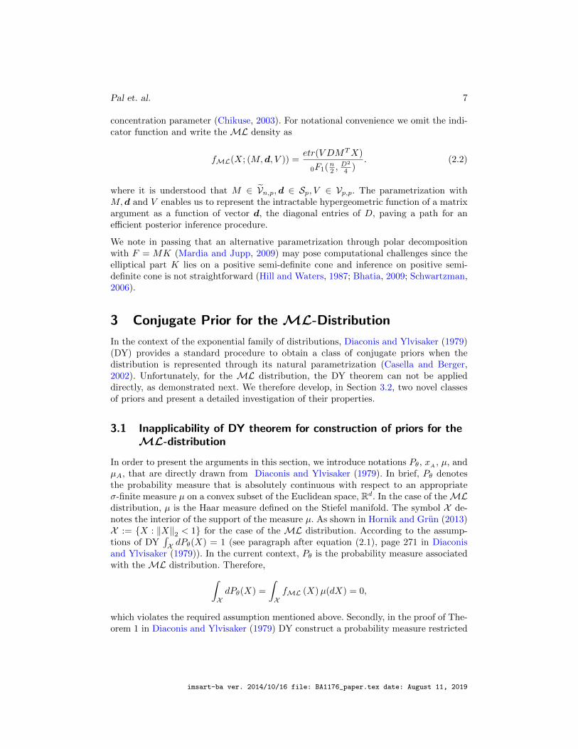

10
(b) If Ψ2 gt 1 thenintVnp
intVpp
intRp+g(Md V νΨ) dmicro1(d) dmicro2(V ) dmicro(M) =infin
where g(Md V νΨ) is defined in Definition 1
The conditions mentioned in this theorem do not span all cases we have not addressedthe case where Ψ2 = 1 As far as statistical inference for practical applications isconcerned we may not have to deal with the case where Ψ2 = 1 as the hyper-parameter selection procedure (see Section 4) and posterior inference (even in the caseof uniform improper prior see Section 53 ) only involve cases with Ψ2 lt 1 Wetherefore postpone further investigation into this case as a future research topic oftheoretical interest
Theorem 2 Let d isin Rp+ η = (η1 ηp) isin Rp and n be any integer with n ge p Thenfor any ν gt 0 int
Rp+g(d νη n) dmicro1(d) ltinfin
if and only if max1lejlep
ηj lt 1 where g(d νη n) is as defined in Definition 2
We can alternatively parametrize the CCPD class of densities by the following specifi-cation of the probability density function
f(d νη) propexp
(sumpj=1 ηjdj
)[0F1(n2
D2
4 )]ν
where max1lejlep ηj lt ν In this parametrization if we consider the parameter choicesν = 0 and β = minusη then the resulting probability distribution corresponds to theExponential distribution with rate parameter β
It is important to explore the properties for the CCPD and JCPD class of distributionsin order to use them in an effective manner Intuitive interpretations of the parametersνηΨ are desirable for example for hyper-parameter selection Due to conjugacyBayesian analysis will lead to posterior distributions involving JCPD and CCPD andtherefore it is necessary to identify features that are required to develop practicablecomputation schemes for posterior inference The following four theorems establish somecrucial properties of the CCPD and JCPD class of distributions
Theorem 3 Let d sim CCPD(middot νη) for ν gt 0 and max1lejlep ηj lt 1 where η =(η1 ηp) Then
(a) The distribution of d is log-concave
imsart-ba ver 20141016 file BA1176_papertex date August 11 2019
Pal et al 11
(b) The distribution of d has a unique mode if ηj gt 0 for all j = 1 2 middot middot middot p The modeof the distribution is given by mη = hminus1(η) where the function h(d) is defined as
follows h(d) = (h1(d) h2(d) middot middot middot hp(d))T
with
hj(d) =
(part
partdj0F1
(n
2D2
4
))0F1
(n
2D2
4
)
Notably the mode of the distribution is characterized by the parameter η and doesnot depend on the parameter ν The proof of the theorem relies on a few nontrivial
properties of 0F1
(n2
D2
4
) ie the hyper-geometric function of a matrix argument
that we have established in the supplementary material Section 1 It is easy to seethat the function hminus1 is well defined as the function h is strictly increasing in all itscoordinates Even though subsequent theoretical developments are based on the formaldefinition and theoretical properties of hminus1 and h functions numerical computation ofthe functions are tricky The evaluation of the functions depend on reliable computation
of 0F1
(n2
D2
4
)and all its partial derivatives In Section 62 we provide a reliable and
theoretically sound computation scheme for these functions
On a related note it is well known that log-concave densities correspond to unimodaldistributions if the sample space is the entire Euclidean space (Ibragimov 1956 Dhar-madhikari and Joag-Dev 1988 Doss and Wellner 2016) However the mode of thedistribution may not necessarily be at a single point Part(b) of Theorem 3 asserts thatthe CCPD has a single point mode Moreover the sample space of CCPD is d isin Rp+which merely encompasses the positive quadrant and not the whole of the p dimensionalEuclidean space Hence general theories developed for Rp (or R) do not apply In factwhen ηj le 0 the density defined in Definition 2 is decreasing as a function of dj on theset R+ and the mode does not exist as R+ does not contain the point 0 In all part(b)of Theorem 3 does not immediately follow from part(a) and requires additional effortto demonstrate
In order to introduce the notion of ldquoconcentrationrdquo for the CCPD class of distributionswe require the concept of a level set Let the unnormalized probability density functionfor the CCPD class of distributions g(x νη) (See Definition 5) achieve its maximumvalue at mη ( part(b) of Theorem 3 ensures that mη is a unique point) and let
Sl =x isin Rp+ g(x 1η)g(mη 1η) gt l
(35)
be the level set of level l containing the mode mη where 0 le l lt 1 To define the levelset we could have used g(x ν0η) for any fixed value of ν0 gt 0 instead of g(x 1η)However without loss of generality we choose ν0 = 1
Let Pν(middotη) denote the probability distribution function corresponding to the CCPD(middot νη)distribution According to Theorem3 for a fixed η isin Rp all distributions in the classPν(middotη) ν gt 0 have the mode located at the point mη
imsart-ba ver 20141016 file BA1176_papertex date August 11 2019
12
Theorem 4 Let dν sim CCPD(middot νη) for a fixed η isin Rp with mη being the mode ofthe distribution If Pν(middotη) denotes the probability distribution function correspondingto dν then
(a) Pν(Slη) is an increasing function of ν for any level set Sl with l isin (0 1)
(b) For any open set S sub Rp+ containing mη Pν(d isin Sη) goes to 1 as ν rarrinfin
The major impediment to proving Theorem 4 arises from the intractability of the nor-malizing constant of the CCPD(middot νη) distribution Although involved the proof es-
sentially uses the log convexity of 0F1
(n2
D2
4
)to get around this intractability
From Theorem 4 it is clear that the parameter ν relates to the concentration of theprobability around the mode of the distribution Larger values of ν imply larger con-centration of probability near the mode of the distribution
Definition 3 In the context of the probability distribution CCPD (middot η ν) the param-eters η and ν are labeled as the ldquomodal parameterrdquo and the ldquoconcentration parameterrdquorespectively
In Figure 1 we display three contour plots of the CCPD(middot νη) distribution with η =(085 088) Note that the corresponding mode of the distribution is hminus1(085 088) =(7 5) for all three plots We can observe the implication of part (b) of Theorem 3 asthe ldquocenterrdquo of the distributions are the same Contrastingly it can be observed thatthe ldquospreadrdquo of the distributions decrease as the value of the parameter ν increases asimplied by Theorem 4
Theorem 5 Let (Md V ) sim JCPD(middot νΨ) for some ν gt 0 and Ψ2 lt 1 If Ψ =MΨDΨV
TΨ is the unique SVD of Ψ with dΨ being the diagonal elements of DΨ then
the unique mode of the distribution is given by (MΨhminus1(dΨ) VΨ) where the function
drarr h(d) is as defined in Theorem 3
Note that the mode of the distribution is characterized by the parameter Ψ and doesnot depend on the parameter ν The proof of the theorem depends crucially on a strongresult a type of rearrangement inequality proved in Kristof (1969)
For the concentration characterization of JCPD we define the level sets in the contextof the JCPD distribution Let the unnormalized probability density function for theJCPD class of distributions g(Md V νΨ) achieve its maximum value at the point
(M d V ) ( see Theorem 5 ) and
Al =
(Md V ) isin Vnp times Rp+ times Vpp g(Md V 1Ψ)g(M d V 1Ψ) gt l
be the level set of level l from some l isin (0 1) The following theorem characterizes theconcentration property of the JCPD distribution
imsart-ba ver 20141016 file BA1176_papertex date August 11 2019
Pal et al 13
Theorem 6 Let (Md V ) sim JCPD(middot νΨ) where Ψ2 lt 1 If Pν(middot Ψ) denotes theprobability distribution function corresponding to the distribution JCPD(middot νΨ) then
(a) Pν(Al Ψ) is a strictly increasing function of ν for any level set Al with l isin (0 1)
(b) For any open set A sub Vnp times Rp+ times Vpp containing the mode of the distributionPν(A Ψ) tends to 1 as ν rarrinfin
(c) The conditional distribution of M given (d V ) and V given (Md) areML distribu-tions whereas the conditional distribution of d given (MV ) is a CCPD distribution
Parts (a) and (b) of the above theorem characterize the concentration whereas part(c)relates CCPD to the JCPD class of distributions Part(c) also motivates the develop-ment of a sampling procedure for the JCPD distribution The proof of part(a) Theo-rem 6 is similar to that of the proof of Theorem 4 The proof for part(b) of Theorem 6is more involved and depends on several key results including the rearrangement in-
equality by (Kristof 1969) the log convexity of 0F1
(n2
D2
4
) and the the fact that
g(hminus1(η) νη)) the value of the unnormalized CCPD density at the mode is astrictly increasing function of the parameter η
Note that unlike in the case of the CCPD distribution we do not attempt to establishthe log concavity of JCPD the reason being that the underlying probability spaceVnp times Rp+ times Vpp is non-convex Nevertheless it is evident that beyond a certain dis-tance (based on a suitable metric on Vnp times Rp+ times Vpp) the value of the density dropsmonotonically as one moves farther away from the center Based on the characteristicsof the parameters ν and Ψ of the JCPD class of distributions we have the followingdefinitions
Definition 4 The parameters Ψ and ν in the distribution JCPD are labeled theldquomodalrdquo parameter and the ldquoconcentrationrdquo parameter respectively
Interestingly both distributions CCPD and JCPD are parameterized by two param-eters one controlling the center and the other characterizing the probability concen-tration around that center One may therefore visualize the distributions in a fashionsimilar to that of the multivariate Normal distribution controlled by the mean andvariance parameters This intuitive understanding can help practitioners select hyper-parameter values when conducting a Bayesian analysis with the CCPD and JCPDdistributions
Thus far we have established properties of CCPD and JCPD that relate to basicfeatures of these distributions Additional properties which are required for a MCMCsampling scheme are developed in Section 51
imsart-ba ver 20141016 file BA1176_papertex date August 11 2019
14
(a) ν = 10 (b) ν = 20 (c) ν = 35
Figure 1 Density plots of CCPD(middot νη) for different values of ν where η = (089 085)Mode of the distributions are located at the point (7 5)
4 Hyperparameter Selection Procedure
41 Informative Prior
We now present procedures for the selection of hyperparameter values aimed at incor-porating prior beliefs about the parameters (Md V ) Consider the scenario where apractitioner has the prior belief that the values for the parameters Md V are closeto Mbelief dbelief Vbelief respectively A standard approach to incorporating this priorknowledge is to select the hyper-parameter values in such a manner that the mode of thecorresponding prior distribution becomes Mbelief dbelief Vbelief In order to achieve thisin the current context we first compute η = h(dbelief ) where h(middot) is defined in Equa-tion 28 in the supplementary material Note that we always get a feasible η for everyreal dbelief isin Sp
In the case of the CCPC class of priors we choose η = η ξM = Mbelief γM = Vbelief ξV = Ip γ
V = Ip in the Equation 34 Theorem 3 guarantees that the above hyper-parameter specifications yields a prior distribution that has mode at (Mbelief dbelief Vbelief )From Theorem 3 we also see that larger values of the hyper-parameter ν lead to largerconcentration of the prior probability around the mode The hyper-parameters ξD andγD play a similar role for the ML distribution Hence the hyper parameters ν ξD andγD are chosen to have larger values in case the practitioner has a higher confidence inthe prior belief
In the case of the JCPC class of priors we apply Theorem 5 to construct JCPD(see Equation 32) with mode at Mbelief dbelief Vbelief In particular we set Ψ =MbeliefDη(Vbelief )T where Dη is the diagonal matrix with diagonal elements η =h(dbelief ) Using the concentration characterization described in Theorem 5 the prac-titioner may choose the value of the hyper-parameter ν appropriately where a largervalue for the parameter ν implies greater confidence in the prior belief
imsart-ba ver 20141016 file BA1176_papertex date August 11 2019
Pal et al 15
It is noteworthy that for both the JCPC and CCPC class of priors there is an intimateconnection between the sample size and the interpretation of the hyper-parameter νAs a heuristic one may envisage ν as incorporating ldquoinformationrdquo equivalent to ν manyhistoric observations of the model
42 Uniform improper prior
In the case where the practitioner does not have a prior belief about the parametervalues an automatic procedure for hyper-parameter selection can be helpful In thisand the next subsection we discuss two automatic procedures to select the values ofthe hyper-parameters In the absence of prior information usage of uniform prior iscommon in the literature In the context of the current model for the JCPC andCCPC class of distributions the prior for the parameters (Md V ) is called a uniformprior if
g(Md V νΨ) prop 1 and
fML(M ξM ξD ξV )g(d νη)fML(V γM γD γV ) prop 1
Both classes of priors JCPC and CCPC are flexible enough to accommodate a uniformprior For JCPC this can be achieved by setting ν = 0 in Equation 32 Correspondinglyfor the CCPC class the uniform prior can be constructed by choosing ν = 0 ξD = 0 andγD = 0 in Equation 34 Note that the resulting uniform prior is improper in nature asthe above choices of hyper parameters do not lead to a proper probability distributionHence it is necessary to check the propriety of the resulting posterior (see Section 53for more details)
43 Empirical prior
Another widely used automatic method is to use empirical information contained inthe data to select appropriate values of the hyper-parameters Let W1W2 WN beindependent and identically distributed samples drawn fromML(middot Md V ) Consider
the sample mean W = (sumNi=1Wi)N Let the unique SVD of the sample mean be
W = MWDWVW Construct candidate values Mbelief = MW Vbelief = VW and η asthe diagonal elements of DW One can set Ψ = W as the hyper-parameter in the caseof the JCPC prior In the case of the CCPC class of priors one can choose η = η andfor the hyper-parameters related to M and V apply the same procedure as discussedpreviously in this section For both classes of priors a value for ν that is less than orequal to 10 percent of the sample size N is recommended
Example 1 Let the practitioner have the following prior belief for the values of the
imsart-ba ver 20141016 file BA1176_papertex date August 11 2019
16
parameters Md V
Mbelief =
1 00 10 0
dbelief =
[75
] Vbelief =
[1 00 1
]
As described previously in this section we can compute η = h(7 5) = (089 085)Hence for the JCPC class of priors we choose the hyper-parameter values
Ψ =
1 00 10 0
[089 00 085
] [1 00 1
]T=
089 00 0850 0
to ensure that JCPD(middot Ψ ν) has mode at Mbelief dbelief Vbelief for all values of ν gt 0The value of the hyper-parameter ν should be chosen according to the strength of theprior belief In Figure 1 we display the resulting conditional distribution for d givenMV Figure 1 shows that the ldquocenterrdquo of the distribution is located at (7 5) Figure 1also displays the ldquospreadrdquo of the distribution around the mode when using ν = 10 ν = 20and ν = 35
5 Properties of Posterior
The derivation of the posterior distributions for the JCPC and CCPC class of priorsis straightforward since they were built with conjugacy in mind which then entailsthat the posterior distributions lie in the corresponding classes However inference forthe resulting posterior distributions is challenging because not only are the normalizingconstants intractable for both the JCPD and CCPD distributions but also the un-
normalized version of the corresponding density functions involve 0F1
(n2
D2
4
) We first
focus our attention on developing properties of the posterior distribution when involvingJCPC and CCPC priors In particular we derive explicit forms of the posterior con-ditionals under different prior settings the linearity of the posterior mode parametersand the strong consistency of the posterior mode
51 Posterior conditionals
Let W1W2 WN be independent and identically distributed samples drawn fromML(middot Md V ) Let W =
sumNi=1WiN The likelihood of the data is
Nprodi=1
etr(V DMTWi)
0F1(n2 D2
4 ) (51)
First let us assume a JCPD prior with parameters ν and Ψ Theorem 5 not onlyimplies that the posterior has a unique mode but also provides an expression for the
imsart-ba ver 20141016 file BA1176_papertex date August 11 2019
Pal et al 17
mode Furthermore we see that the corresponding posterior distribution is JCPD with
concentration (ν +N) and posterior modal parameter ΨN =(
νν+NΨ + N
ν+NW) Let
ηΨN be the diagonal elements of the diagonal matrix DΨN where ΨN = MN DΨN VN is
the unique SVD for ΨN From Theorem 6 it follows that the full posterior conditionalsfor the parameters Md V are ML CCPD and ML distributions respectively
In Section 6 we shall use these results to construct a Gibbs algorithm A part of theGibbs scheme would require sampling from the relevant CCPD distribution which wepropose to implement by simulating from the full conditional distribution of each of thecomponents of d given the rest when d sim CCPD(middot νη) To refer to this conditionaldistribution in subsequent text we have the following definition
Definition 5 Let ν gt 0 $ isin Rpminus1+ and η isin Rp+ with max1lejlep ηj lt 1 A random vari-
able is defined to be distributed as CCPDj (middot $ νη) if the corresponding probability
density function (with respect to the Lebesgue measure on R) is proportional to
gj(x $ νη) =exp(ν ηjx)[
0F1
(n2
(∆(x))2
4
)]ν where ∆(x) is a diagonal matrix with diagonal elements (x$) isin Rp+
Let d = (d1 dp) be a random vector with d sim CCPD (middot νη) for some max1lejlep ηj lt1 ν gt 0 Let d(minusj) be the vector containing all but the j-th component of the vector dThen the conditional distribution of dj given d(minusj) is CCPD
j (middot d(minusj) νη) ie
dj | d(minusj) sim CCPDj (middot d(minusj) νη)
Now since the conditional posterior of d was shown to be CCPD the conditionalposterior distribution of dj | d(minusj)M V WiNi=1 follows a CCPD
j distribution
In the case of a Bayesian analysis with a CCPC prior Equation 34 and 51 determinethe corresponding posterior distribution to be proportional to
etr((V DMT
)N W +G0M +H0 V
)0F1(n2 D24)ν+N
exp(ν ηTd) (52)
where G0 = ξV ξD (ξM )T
and H0 = γV γD (γM )T
The conditional probability density
for the posterior distribution of d given M V WiNi=1 is proportional to
exp
((ν +N)
(ν
ν+N η + Nν+N ηW
)Td
)[0F1
(n2
D2
4
)]ν+N (53)
imsart-ba ver 20141016 file BA1176_papertex date August 11 2019
18
where ηW = (Y11 middot middot middot Ypp) with Y = MTWV It follows that the conditional posteriordistribution of d given MV WiNi=1 is CCPD(middot νN ηN ) where νN = ν + N and
ηN =(
νν+N η + N
ν+N ηW
) The conditional posterior distributions M | d V WiNi=1
and V | dM WiNi=1 are ML distributions
52 Linearity of posterior modal parameter
We observe that the posterior modal parameter is a convex combination of the priormodal parameter and the sample mean when applying the JCPC class of priors Inparticular from Section 51 we get
ΨN =
(ν
ν +NΨ +
N
ν +NW
)
In a similar fashion we observe from Equation 53 that the modal parameter for theconditional posterior distribution of d given MV WiNi=1 is a convex combination ofthe prior modal parameter and an appropriate statistic of the sample mean We shouldpoint out here that the posterior linearity of the natural parameter of an exponentialfamily distribution directly follows from Diaconis and Ylvisaker (1979) However in ourparametrization the ML density is a curved exponential family of its parameters andposterior linearity appears to hold for the ldquomodal parameterrdquo
53 Posterior propriety when using uniform improper prior
In the case where a uniform improper prior is used the corresponding posterior isproportional to
etr(N VDMTW
)[0F1(n2
D2
4 )]N (54)
where W = 1N
sumNi=1Wi (see Equation 51) It follows from Theorem 1 that the function
in Equation 54 leads to a proper distribution JCPD(middot NW ) if∥∥W∥∥
2lt 1 The
following theorem outlines the conditions under which∥∥W∥∥
2lt 1
Theorem 7 Let W1 WN be independent and identically distributed samples froman ML-distribution on the space Vnp If
(a) N ge 2 p lt n
(b) N ge 3 p = n ge 3
then∥∥W∥∥
2lt 1 with probability 1 where W = 1
N
sumNi=1Wi
imsart-ba ver 20141016 file BA1176_papertex date August 11 2019
Pal et al 19
54 Strong consistency of the posterior mode
In the case where we use a JCPD(middot νΨ) prior for Bayesian analysis of the data WiNi=1the corresponding posterior distribution is a JCPD with concentration ν +N and poste-
rior modal parameter ΨN =(
νν+NΨ + N
ν+NW)
(See Section 51) Let ΨN = MΨDΨVTΨ
be the unique SVD of ΨN with dΨ being the diagonal elements of DΨ Then from The-orem 5 the unique mode of the distribution is given by (MN dN VN ) where
MN = MΨ dN = hminus1(dΨ) and VN = VΨ
The form of the function h(d) is provided in Theorem 3 The nontrivial aspect offinding the posterior mode is the computation of the function hminus1(dΨ) In our ap-plications we use a Newton-Raphson procedure to obtain hminus1(dΨ) numerically We
use large and small argument approximations for 0F1
(n2
D2
4
)( See Jupp and Mardia
(1979)) to initialize the Newton-Raphson algorithm for faster convergence Note thatthe success of the Newton-Raphson procedure here depends on the efficient computa-
tion of 0F1
(n2
D2
4
)and its partial derivatives In Section 62 we provide a method to
compute these functions reliably
The following theorem demonstrates that the mode of the posterior distribution is astrongly consistent estimator for the parameters Md V
Theorem 8 Let W1 WN be independent and identically distributed samples fromML(middot Md V ) Let MN dN and VN be the posterior mode when a JCPC prior isused The statistic MN DN and VN are consistent estimators for the parameters MDand V Moreover
(MN dN VN )asminusrarr (Md V ) as N minusrarrinfin
where as stands for almost sure convergence
6 MCMC sampling from the Posterior
Apart from finding the posterior mode a wide range of statistical inference proceduresincluding point estimation interval estimation (see Section 8) and statistical decisionmaking (see Section 8) can be performed with the help of samples from the posteriordistribution For the JCPD and CCPD classes of distributions neither is it possibleto find the posterior mean estimate via integration nor can we directly generate iidsamples from the distributions We therefore develop procedures to generate MCMCsamples using a Gibbs sampling procedure which requires the results on posterior con-ditionals stated in Section 51
It follows from Theorem 6 and Section 51 that under JCPD prior the conditionaldistribution of M given d V and the conditional distribution of V given Md are MLdistributions while the conditional distribution of d given MV is CCPD Conse-quently the conditional distribution of dj | d(minusj)M V WiNi=1 follows a CCPD
j dis-
tribution (see Definition 5) Also let us assume that the unique SVD for νN (ΨNV D) =
imsart-ba ver 20141016 file BA1176_papertex date August 11 2019
20
MMΨDM
Ψ(VM
Ψ)T
and for νN (ΨTNMD) = MV
ΨDV
Ψ(V V
Ψ)T
Also let us denote the vector
containing the diagonal element of the matrix MT ΨNV to be ηΨ Based on the abovediscussion we can now describe the algorithm as follows
Algorithm 1 Gibbs sampling algorithm to sample from posterior when using JCPCprior
1 Sample M | d V WiNi=1 simML(middot MM
ΨdM
Ψ VM
Ψ
)
2 Sample dj | d(minusj)MV WiNi=1 sim CCPDj
(middot d(minusj) νN ηΨ
)for j = 1 p
3 Sample V | d V WiNi=1 simML(middot MV
ΨdV
Ψ V V
Ψ
)
If instead we use a CCPC prior (see Equation 34) for Bayesian analysis of the datathen the full conditional distribution of Md V areML CCPD andML distributionsrespectively The steps involved in the Gibbs sampling Markov chain are then as follows
Algorithm 2 Gibbs sampling algorithm to sample from posterior when using CCPCprior
1 Sample M | d V WiNi=1 simML(middot SMG SDG SVG
)
2 Sample dj | d(minusj)M V WiNi=1 sim CCPDj
(middot d(minusj) νN ηN
)for j = 1 p
3 Sample V |Md WiNi=1 simML(middot SMH SDH SVH
)
where νN ηN are defined in Equation 53 and (SMG SDG S
VG ) (SMH S
DH S
VH) are the
unique SVD of the matrices (DV T NWT
+G0) and (DV T NWT
+H0) respectively
To implement the above algorithms we need to sample from the ML and CCPD dis-tributions For the former we use the procedure developed in (Hoff 2009) to samplefrom the ML distributions Sampling from CCPD
j is much more involved and is ex-plained in detail in the next subsection The following result provides some theoreticalguarantees that shall be useful for this specific sampler
Theorem 9 Let d sim CCPD(middot νη) for some ν gt 0 and η = (η1 ηp) wheremax1lejlep ηj lt 1 Let g1(middot d(minus1) νη) denote the unnormalized density correspondingto CCPD
1(middot d(minus1) νη) the conditional distribution of d1 given (d2 dp)
(a) The probability density function corresponding to CCPD1(middot d(minus1) νη) is log-
concave on the support R+
(b) If 0 lt η1 lt 1 the distribution CCPD1(middot d(minus1) νη) is unimodal and the mode
of the distribution is given by m where h1(m) = η1 If η1 le 0 then the probabilitydensity is strictly decreasing on R+
(c) If B gt m is such that g1(Bd(minus1)νη)g1(md(minus1)νη)
lt ε for some ε gt 0 then P (d1 gt B |d2 dp) lt ε
imsart-ba ver 20141016 file BA1176_papertex date August 11 2019
Pal et al 21
(d) Let Mcrit be any positive number then for all d1 gt Mcrit
g1(d1 d(minus1) νη) le KdaggernpMcritdν(nminus1)21 exp( minusν(1minus η1) d1)
(61)
where
KdaggernpMcrit=
[(p4)
n2minus12 )
Γ(n2)radic
Mcric eminusMcrit In2minus1(Mcrit)]ν
Even though parts (a) and (b) of the above theorem follow immediately from Theorem 3they are included here for completeness all the properties play a crucial role in theconstruction of the sampling technique for CCPD
j The proof of part(c) is essentiallyan implication of the fact that the right tail of the distribution decays at an exponential
rate To show part(d) we have developed a nontrivial lower bound for 0F1
(n2
D2
4
)
Remark 1 The constant KdaggernpMcritin part(d) of Theorem 9 converges to a finite con-
stant as Mcrit approaches infinity It follows from the properties of the Bessel functionthat
limMcritrarrinfin
radicMcrite
minusMcritIaminus1(Mcrit) =1radic2π
for all a ge 32 Hence for larger values of Mcrit the value of KdaggernpMcrit
approaches[radic2π(p4)
n2minus12 )
Γ(n2)
]ν a nonzero finite constant depending on n p ν
Note that the ratio g1(B d(minus1) νη)g1(m d(minus1) νη) mentioned in part(c) is freeof the intractable normalizing constants of the distribution Therefore the numeri-cal computation of the ratio is possible as long as we can compute the corresponding
0F1
(n2
D2
4
) Using Theorem 9 we develop an accept-reject sampling algorithm that
can generate samples from CCPDj with high acceptance probability The detailed con-
struction of the sampler is provided next We conclude this section with a description
of an efficient procedure for computing the 0F1
(n2
D2
4
)constant
61 A rejection sampler for the CCPDj distribution
We now describe a rejection sampling procedure from the conditional distribution of(d1 | (d2 middot middot middot dp)) when d sim CCPC (middot νη) for some ν gt 0 and max
1lejlepηj lt 1 Here
η = (η1 ηp) Let m be the mode of the conditional distribution g1(middot) = g(middot νη |(d2 dp)) of the variable d1 given (d2 dp) when η1 gt 0 In case η1 le 0 we set mto be 0 Using the properties of the conditional distribution described in Theorem 9 we
compute a critical point Mcrit such that P(d1 gt Mcrit | (d2 middot middot middot dp) XjNj=1
)lt ε
Here we have chosen ε = 00001
imsart-ba ver 20141016 file BA1176_papertex date August 11 2019
22
To construct a proposal density g1(x) we employ two different strategies one for the
bounded interval (0Mcrit] and the other using Theorem 9 to tackle the tail (Mcritinfin)
of the support of the conditional posterior distribution of d1
The procedure is as follows Let δ = McritNbin where Nbin is the total number of
partitions of the interval (0Mcrit] Consider k = ([mδ] + 1) where [mδ] denotes the
greatest integer less than or equal to mδ Now define the function
g1(x) =
kminus1sumj=1
g1(j δ) I((jminus1)δjδ])(x) + g1(m)I((kminus1)δkδ])(x)
+
Nbinsumj=k+1
g1((j minus 1) δ) I(((jminus1)δjδ])(x)
+KdaggernpMcritdν(nminus1)21 exp( minusν(1minus η1) d1)I(Mcritinfin))(x) (62)
where KdaggernpMcritis as defined in part(d) of Theorem 9
From Theorem 9 it follows that g1(x) ge g1(x) for all x gt 0 as g1(middot) is a unimodal
log-concave function with maxima at m We consider
qj =
δ g1(jδ) if 1 le j lt
[mδ
]+ 1
δ g1(m) if j =[mδ
]+ 1
δ g1((j minus 1)δ) if[mδ
]+ 1 lt j le Nbin
KdaggernpMcrit
Γ( (ν(nminus1)+2)2 Mν(1minusη1))
[ν(1minusη1)]ν(nminus1)2+1 if j = Nbin + 1
where Γ(
(ν(nminus1)+2)2 Mcritν(1minus η1)
)denotes the upper incomplete gamma function
For the case where Mcrit tends toinfin (see Remark 1) the constant KdaggernpMcritapproaches
a finite constant whereas Γ(
(ν(nminus1)+2)2 Mcritν(1minus η1)
)monotonically decreases to
zero Therefore the positive constant qNbin+1
can be made arbitrary close to zero by
choosing a suitably large value for Mcrit when the value of n p ν η1 are fixed Note that
the quantities qjNbin+1j=1 may not add up to 1 therefore we construct the corresponding
set of probabilities pjNbin+1j=1 where pj = qj
sumNbin+1j=1 qj for j = 1 2 middot middot middot Nbin+1 The
following algorithm lists the steps involved in generating a sample from the distribution
corresponding to the kernel g1(middot)
imsart-ba ver 20141016 file BA1176_papertex date August 11 2019
Pal et al 23
Algorithm 3 Steps for the rejection sampler for CCPDj
1 Sample Z from the discrete distribution with the support 1 2 (Nbin+1) andcorresponding probabilities pjNbin+1
j=1 2 if Z le Nbin then3 Sample y sim Uniform ((Z minus 1) δ Zδ)
4 else Sample y sim TruncatedGamma(
shape = ν(nminus1)+22 rate = ν(1minus η1) support = (Mcritinfin)
)5 end if6 Sample U sim Uniform (0 1)
7 if U le g1(y)g1(y) then
8 Accept y as a legitimate sample from g1(middot)9 else Go to Step 1
10 end if
Figure 2 shows a typical example of the function g1(x) and the corresponding g1(x)The blue curve represents the unnormalized density g1 The black curve and the redcurve after Mcrit constitutes the function g1 ( defined in Equation 62) Note that the
red curve after the point Mcrit represents the last term (involving KdaggernpMcrit) in the
summation formula in Equation 62 In Figure 2(a) the values of δ and Mcrit are setsuch that the key components of g1 and g1(x) are easy to discern On the other handFigure 2(b) displays the plot of g1(x) when recommended specification of Mcrit and δare used
M_Crit
0
50
100
150
200
250
5 10 15
Support of the distribution
dens
ity
M_Crit
0
50
100
150
200
250
5 10 15
Support of the distribution
dens
ity
(a) (b)
Figure 2 The blue curves represent g1 the unnormalized density of CCPD1 distri-
butions The black curve and the red curve after Mcrit constitutes the function g1the proposal density for the accept reject algorithm The panel(a) displays the key as-pects of the densities while panel(b) shows the proposal density when recommendedspecifications of Mcrit and δ are used
The choice of Nbin plays a crucial role in the algorithm and is required to be determinedbefore constructing the proposal density for the accept-reject algorithm Note that Nbin
imsart-ba ver 20141016 file BA1176_papertex date August 11 2019
24
and δ are interconnected If one is specified the value of the other can be determinedWe decide to choose the parameter δ and compute the corresponding Nbin In the casewhere the concentration parameter is high a finer partition of the proposal histogram(smaller value of δ) is required to keep the acceptance rate of the algorithm high Basedon our empirical results we recommend selecting δ to be of the order of 1radic
ν The
acceptance probability remains stable across different choices of ν when the value δ isset accordingly (see Figure 3) The estimated acceptance probabilities used in Figure 3were calculated based on 10000 Monte Carlo samples for each value of ν varied from 1to 100 The relationship between Nbin and δ and ν is presented in Table 1
Finally successful implementation of the sampling algorithm developed in this subsec-
tion requires the computation of 0F1
(n2
D2
4
) a key step for the computation of g1(middot)
In Section 62 we discuss the procedure that we have adopted to compute 0F1
(n2
D2
4
)
0 20 40 60 80 100
080
085
090
095
100
Concentration
Est
imat
ed A
ccep
tenc
e P
roba
bilit
y
Figure 3 Estimated acceptance probability of the sampling algorithm when the valueof the concentration parameter varies from 1 to 100 The parameter δ is chosen to bereciprocal of
radicν
62 Computation of 0F1
(n2 D
2
4
)We first describe an efficient and reliable computational procedure to compute the
function 0F1
(n2
D2
4
)when the argument matrix D is of dimension 2times2 The procedure
is relevant to many applications considered in the field (Downs et al 1971 Downs 1972Jupp and Mardia 1979 1980 Mardia and Khatri 1977 Mardia et al 2007 Mardiaand Jupp 2009 Chikuse 1991ab 1998 2003 Sei et al 2013 Lin et al 2017) We
imsart-ba ver 20141016 file BA1176_papertex date August 11 2019
Pal et al 25
ν δ Estimated Acceptance probability Nbin1 1 095813 421 05 0977517 851 0333333 0984155 1271 02 0988924 2121 01 0996314 4251 005 0998104 8513 05 0952835 273 0333333 0963206 403 02 0977326 673 01 0988924 1353 005 0995124 2715 1 0885818 35 05 0941886 75 0333333 0960246 105 02 0973994 175 01 0989218 355 005 0993246 71
Table 1 Values of the Nbin δ and acceptance probability for algorithm to generatevalues from CCPDj(η ν) for ν = 1 3 5
emphasize that the computational procedure described below is applicable for analyzingdata on Vn2 for all n ge 2
Consider the representation developed in Muirhead (1975) for the Hypergeometricfunction of a matrix argument
0F1 (cD) =
infinsumk=0
dk1dk2(
cminus 12
)k
(c)2k k0F1 (c+ 2k d1 + d2) (63)
where D is a 2times 2 diagonal matrix with diagonal elements d1 gt 0 d2 gt 0 From Butlerand Wood (2003) (see page 361) it can be seen that
0F1 (c+ 2k d1 + d2) =Γ (c+ 2k)(radic
d1 + d2
)(c+2kminus1)Ic+2kminus1
(2radicd1 + d2
) (64)
where Ic+2kminus1(middot) is the modified Bessel function of the first kind with order (c+2kminus1)Hence from Equation 63 and Equation 64 we get that
0F1 (cD) =
infinsumk=0
dk1dk2(
cminus 12
)k
(c)2k k
Γ (c+ 2k) Ic+2kminus1
(2radicd1 + d2
)(radicd1 + d2
)(c+2kminus1)
=
infinsumk=0
Ak (65)
imsart-ba ver 20141016 file BA1176_papertex date August 11 2019
26
where Ak = Γ(cminus5)Γ(c)Γ(c+kminus5)k
(d1d2)k
(radicd1+d2)
(c+2kminus1) Ic+2kminus1
(2radicd1 + d2
) Note that
Ak+1
Ak=
Γ(c+ k minus 5)k
Γ(c+ k + 5)(k + 1)
Ic+2k+1
(2radicd1 + d2
)Ic+2kminus1
(2radicd1 + d2
) d1d2
(d1 + d2)
le 4d1d2
(2c+ 2k minus 1)(2k + 2)(2k + c)(2k + 2c+ 1) (66)
where the last inequality follows from Iν+1(x)Iν(x) lt x2(ν+1) for x gt 0 ν gt minus1 (see
page 221 in Ifantis and Siafarikas (1990)) For fixed values of d1 d2 we can find M suchthat AM le ε and M4 ge (d1 d2)(4ε1) for some ε1 lt
12 and a predetermined error bound
ε For such a choice of M if k is any integer such that k geM then
Ak+1
Akle 4d1d2
(2c+ 2k minus 1)(2k + 2)(2k + c)(2k + 2c+ 1)
le 4d1d2
(2c+ 2M minus 1)(2M + 2)(2M + c)(2M + 2c+ 1)
le(d1d2
4M4
)16M4
(2c+ 2M minus 1)(2M + 2)(2M + c)(2M + 2c+ 1)
le
(d1d2
4M4
)M4
(M + 2cminus12 )(M + 1)(M + c
2 )(M + 2c+12 )
le ε1 (67)
where the last inequality follows due to the fact that M4 le (M + 2cminus12 )(M + 1)(M +
c2 )(M + 2c+1
2 ) as c gt 12 Hence from Equation 65 we get that
|0F1 (cD)minusMsumk=0
Ak| =infinsum
k=M+1
Ak le AMinfinsum
k=M+1
εkminusM1 le ε ε11minus ε1
lt ε (68)
Consequently for a given value of the matrix D and an error level ε we can select Maccordingly so that 0F1 (cD) is approximated as
0F1 (cD) asympMsumk=0
dk1dk2(
cminus 12
)k
(c)2k k
Γ (c+ 2k) Ic+2kminus1
(2radicd1 + d2
)(radicd1 + d2
)(c+2kminus1) (69)
where the error in the approximation is at most ε
In the case when the matrix D is of dimension p times p with p gt 2 we rely on the com-putational technique developed in (Koev and Edelman 2006) Development of efficientcomputational schemes for the hyper geometric function of a matrix argument in gen-eral dimension is an active area of research (Gutierrez et al 2000 Koev and Edelman2006 Nagar et al 2015 Pearson et al 2017) In principle the theoretical frameworkdeveloped in this article integrated with the general computation scheme specified inKoev and Edelman (2006) can handle data on Vnp for arbitrary integers n ge p ge 2 butthe results from the combined procedure may lack precision as it inherits the limitations
imsart-ba ver 20141016 file BA1176_papertex date August 11 2019
Pal et al 27
of the algorithm in Koev and Edelman (2006) ( See page 835 in Koev and Edelman
(2006)) In the following remark we specify the assumptions under which the combined
procedure can be applied effectively
Remark 2 The algorithm developed in Koev and Edelman (2006) is a general pro-
cedure for computing pFq(middot) for arbitrary integers p q ge 0 Naturally the algorithm
applies to 0F1 which is the object of focus in the current context Due to its generality
the computational scheme has certain limitations In particular it requires appropri-
ate specification of a ldquotuning parameterrdquo that can not be determined in an automated
manner However from an empirical exploration of the procedure we observed that the
corresponding outputs can be quite robust Particularly the output was found to stabilize
after a certain point (we will call this the ldquostabilization pointrdquo) when the value of the
tuning parameter was gradually increased For the case of p = 2 if the tuning parameter
is specified to be larger than the stabilization point the output from Koev and Edelman
(2006) is very close to the true value as determined by our arbitrary precision algo-
rithm Extrapolating to p ge 3 we presume that the true value of the corresponding hyper
geometric function will be close to the output of Koev and Edelman (2006) if the tuning
parameter is set larger than the ldquostabilization pointrdquo As the ldquostabilization pointrdquo is ob-
served to be larger for larger values of D we can set the value of the tuning parameter
to a single pre-specified number for an entire analysis only if we assume that the diago-
nal elements of the matrix D are bounded above by a prespecified finite number Under
this assumption we can rely on Koev and Edelman (2006) for the analysis of data on
Vnp n ge p ge 3 In that case the combination of our theoretical framework and the
algorithm for the computation of the hypergeometric function from Koev and Edelman
(2006) would work effectively for practical applications (see Simulation Section72)
In contrast the procedure to compute 0F1
(n2
D2
4
)that we have developed though tar-
geted towards a specific case has a theoretical guarantee for a desired level of precision
of its output Since many statistical applications as mentioned earlier are about an-
alyzing data on Vn2 the computation procedure we have designed specifically for Vn2has its own merit
7 Simulation
To evaluate the performance of the procedure presented in the previous sections we
performed simulation experiments We considered two different setups In the first
we analyzed simulated datasets in Vnp where we varied n to assess its effect on the
posterior estimation efficiency Here the value of p was fixed at 2 and the computation
of 0F1
(n2
D2
4
)developed in Section 62 was utilized In the second setup we analyzed
data on Vnp to demonstrate the generic applicability of our framework by setting p = 3
n = 5 Here we used the procedure in Koev and Edelman (2006) to calculate the value
0F1
(n2
D2
4
)
imsart-ba ver 20141016 file BA1176_papertex date August 11 2019
28
71 Simulation Setup (p = 2)
We present results from experiments with simulated data where we varied the dimensionof the Stiefel manifold n across a range of values The objective of this simulationstudy was to see how the error rates varied with the dimension n Specifically wegenerated 3000 observations usingML distribution on V32 V52 V102 and V152 Thesecorrespond to the Stiefel Manifolds with dimension [n = 3 p = 2] [n = 5 p = 2][n = 10 p = 2] and [n = 15 p = 2] respectively We generated 50 datasets for eachsimulation setting using the algorithm mentioned in Hoff (2009) In order to generatedata for each dataset we fixed the parameters M and V to the canonical orthogonalvectors of appropriate dimension and generated two entries of the parameter D fromtwo independent gamma distributions
We ran posterior inference for each of these datasets using 3000 MCMC samples withan initial 1000 samples as burn-in We used the posterior mean of the parameter F asthe point estimate F Finally we assessed our performance by computing the relativeerror for the estimate of Ftrue = MtrueDtrueV
Ttrue We define the relative error as
F minus FtrueFtrue
where middot denotes the matrix Frobenious norm Figure 4 shows the average relativeerror with the corresponding standard deviation of estimation for V32 V52 V102 andV152 for N = 2000 (panel (a)) and for N = 3000 (panel (b)) The average relative errorsdo not seem to exceed 11 and 9 for N = 2000 and 3000 respectively even with thedimension as high as 15 The error rate tends to increase with higher dimension ievalue of n Also we investigated the relationship with the total sample size and foundthese error rates to decrease with larger sample sizes For example the reduction inaverage relative error rate for n = 5 and N = 2000 is around 2 Overall these resultsdemonstrate the robustness of our inference procedure
72 Simulation Setup (p gt 2)
Having demonstrated the efficiency of our method for a range of values of n with p = 2we now present an example of a generalized simulation scenario for p gt 2 Here weuse the procedure in Koev and Edelman (2006) to numerically approximate the value of
0F1
(n2
D2
4
)where D is a ptimesp dimensional matrix with p gt 2 (See Remark 2) Through
the entire simulation we fixed the tuning parameter required in the computation of
0F1
(n2
D2
4
)to a large prespecified value Here we give a specific example with n = 5
and p = 3 We generated 50 datasets of 500 observations each using theML distributionwith different parameters on V53 We then ran posterior inference for each of thesedatasets using 1100 MCMC samples with an initial 100 sample burn-in We used theposterior mean of the parameter F as before as the estimate of the true parameterF Using the same metric we computed the average relative error of the estimation(Figure 5) We observed that our sampling algorithm for di (i = 1 2 3) runs with a
imsart-ba ver 20141016 file BA1176_papertex date August 11 2019
Pal et al 29
(a) with 2000 data points (b) with 3000 data points
Figure 4 Relative error of F for matrices with different dimensions
001
002
003
0 10 20 30 40 50
dataset
||F_t
rminusF
_est
||^2
||F
_tr|
|^2
For matrices with dim (5x3)
Figure 5 Average relative error for datasets on V53
very low rejection rate As can be seen in Figure 5 the average relative errors do not
exceed 3 demonstrating the general applicability of our framework beyond p = 2
imsart-ba ver 20141016 file BA1176_papertex date August 11 2019
30
Codes for the algorithms are available at httpsgithubcomssra19Stiefel_Bayesgit
8 Application
Finally to showcase the methodology developed in this paper we analyzed the vec-torcardiogram dataset discussed in Downs et al (1971) The dataset contains vector-cardiograms of 56 boys and 42 girls aged between 2 and 19 years Individuals in thedataset are partitioned into four groups groups 1 and 2 consist of boys aged between2 minus 10 and 11 minus 19 years while groups 3 and 4 consist of girls aged between 2 minus 10and 11minus19 years Each sample contains vectorcardiograms acquired using two differentmeasurement systems the Frank lead system (Frank 1956 Downs et al 1971) and theMcFee lead system (Downs et al 1971) Here we restrict ourselves to groups 1 and 3and measurements acquired using the McFee lead system For each individual samplewe considered the pair of orthogonal vectors that provides the orientation of the ldquoQRSlooprdquo (Downs et al 1971) in R3 Each orientation in the sample is defined by a 3 times 2matrix with orthonormal columns ie an element in V32 Additional details regardingthe measurements data structures and data processing can be found in Downs et al(1971)
81 MCMC convergence diagnostics
We ran several MCMC convergence diagnostic tests for the MCMC samples from theposterior of F = MDV T which is the natural parameter of the Matrix Langevin distri-bution The parameter F uniquely identifies and is uniquely identified by the parametersMD V Moreover the elements of the matrix M and V are interrelated whereas thecomponents of F are not thus constrained We therefore focused the diagnostics onF and studied its estimation accuracy As notation Fij denotes the [i j]-th elementof F We first ran convergence diagnostics based on potential scale reduction factor(PSRF) Gelman et al (1992) We ran the MCMC procedure three times with differentrandom seeds for 10 000 MCMC iterations with a 1000 sample burn-in The PSRF is aweighted sum of within-chain and between-chain variances The calculated PSRF was100 with an upper confidence bound 101 indicating no evidence of lack of convergenceWe show how the PSRF changed with the iterations in Figure 6 for all components ofF We also calculated a multivariate potential scale reduction factor (MPSRF) that wasproposed by Gelman and Brooks Brooks and Gelman (1998) The calculated MPSRFwas 101 also confirming that there was no lack of convergence The log-likelihood isyet another measure representative of the multi-dimensional parameters In this casetoo the calculated PSRF for log-likelihood was 10 with an upper confidence bound 10indicating no evidence of lack of convergence Finally we calculated the Heidelberg andWelch (HW) diagnostic Heidelberger and Welch (1981 1983) which is a test statisticbased on the Cramer-von Mises test statistic to accept or reject the null hypothesis thatthe MC is from a stationary distribution This diagnostic has two parts and the MCchain for F passed both the Stationarity and Halfwidth Mean tests This test too thenshowed no evidence for lack of convergence
imsart-ba ver 20141016 file BA1176_papertex date August 11 2019
Pal et al 31
Figures 7(a) 7(b) and 8 show the traceplots autocorrelations and densities of differentcomponents of the posterior samples of F from the three runs respectively Notablythe densities of all the components of F are unimodal confirming convergence
2000 4000 6000 8000 10000
10
15
20
25
last iteration in chain
shrin
k fa
ctor
median975
F_1_1
2000 4000 6000 8000 10000
100
102
104
106
last iteration in chain
shrin
k fa
ctor
median975
F_1_2
2000 4000 6000 8000 10000
100
110
120
last iteration in chain
shrin
k fa
ctor
median975
F_2_1
2000 4000 6000 8000 10000
10
12
14
16
last iteration in chain
shrin
k fa
ctor
median975
F_2_2
2000 4000 6000 8000 10000
10
14
18
22
last iteration in chain
shrin
k fa
ctor
median975
F_3_1
2000 4000 6000 8000 10000
100
105
110
115
last iteration in chain
shrin
k fa
ctor
median975
F_3_2
Figure 6 PSRF for all six components of posterior samples of F
82 Parameter estimation
We modeled the vectorcardiogram dataset usingML distributions on V32 There were28 and 17 observations in groups 1 and 3 respectively We assumed that each iid ob-servation in group 1 follows a ML distribution with parameters Mgroup1dgroup1 andVgroup1 and likewise iid observations in group 3 follow aML distribution with param-eters Mgroup3dgroup3 and Vgroup3 We used the uniform improper prior for estimation of
imsart-ba ver 20141016 file BA1176_papertex date August 11 2019
32
F_3_2
F_3_1
F_2_2
F_2_1
F_1_2
F_1_1
1000 3500 6000 8500
1000 3500 6000 8500
1000 3500 6000 8500
1000 3500 6000 8500
1000 3500 6000 8500
1000 3500 6000 850005
1015
10
20
30
0
5
minus20minus15minus10
minus5
255075
5
10
15
Iteration
valu
e
Chain
1
2
3
1 2 3
F_1_1
F_1_2
F_2_1
F_2_2
F_3_1
F_3_2
0 10 20 30 40 50 0 10 20 30 40 50 0 10 20 30 40 50
minus10
minus05
00
05
10
minus10
minus05
00
05
10
minus10
minus05
00
05
10
minus10
minus05
00
05
10
minus10
minus05
00
05
10
minus10
minus05
00
05
10
Lag
Aut
ocor
rela
tion Chain
1
2
3
(a) traceplots (b) autocorrelations
Figure 7 Traceplots and autocorrelations of all six components of posterior samples ofF from three runs
the parameters related to both groups (see Section 4) From Equation 54 we note thatthe posterior distributions of (Mgroup1dgroup1 Vgroup1) and (Mgroup3dgroup3 Vgroup3)given the data are
JCPD(middot 28 W group1
)and JCPD
(middot 17 W group3
)where
W group1 =
0687 05760551 minus07370122 0142
and W group3 =
0682 05850557 minus07350125 0055
are the sample means of the observations in groups 1 and 3 respectively We verified thespectral norm condition in Theorem 1 for the posterior distributions to be well definedwe found
∥∥W group1
∥∥2
= 0946 and∥∥W group3
∥∥2
= 0941
Using Theorem 3 we can infer that the above-mentioned posterior distributions haveunique modes Also from Theorem 3 we can compute the posterior mode and they were
Mgroup1 =
minus0650 07330743 0668minus0157 0127
dgroup1 =
[163295953
] Vgroup1 =
[minus0059 0998minus0998 minus0059
]
Similarly we can compute the posterior mode for the parameters of group 3 (not re-ported here) To estimate the posterior mean for the parametric functions
Fgroup1 = Mgroup1Dgroup1VTgroup1 and Fgroup3 = Mgroup3Dgroup3V
Tgroup3
imsart-ba ver 20141016 file BA1176_papertex date August 11 2019
Pal et al 33
F_3_2
F_3_1
F_2_2
F_2_1
F_1_2
F_1_1
5 10 15
25 50 75
minus20 minus15 minus10 minus5
0 5
10 20 30
0 5 10 15000005010015020
000
005
010
00
01
02
000005010015
0001020304
000005010015020
value
dens
ity
Chain
1
2
3
Figure 8 Densities of all six components of posterior samples of F from three runs
we ran the MCMC based posterior inference procedure described in Section 6 to generateMCMC samples from each of the posterior distribution
For group 1 the posterior mean for the parametric function Fgroup1 = Mgroup1Dgroup1VTgroup1
was
F group1 =
5183 90863583 minus109960919 2221
SD(F group1) =
1527 23541475 26650596 0898
where the entries of the matrix SD(F group1) provides the standard deviation for the
corresponding entries of F group1 From the MCMC samples we also estimated theposterior density of each entry of Fgroup1 and Fgroup3 Figure 9 shows the corresponding
imsart-ba ver 20141016 file BA1176_papertex date August 11 2019
34
00
01
02
0 5 10
(11) th component of F
000
005
010
015
0 5 10 15 20
(12) th component of F
00
01
02
0 5 10
(21) th component of F
000
005
010
015
minus20 minus15 minus10 minus5
(22) th component of F
00
02
04
06
minus2 0 2 4
(31) th component of F
00
01
02
03
04
minus2 0 2 4 6
(32) th component of F
Figure 9 Estimated posterior density for the parameter F The estimated density forGroup 1 and Group 3 are marked with Red and Blue lines respectively
density plots The estimates related to group 3 were
F group3 =
3249 85473798 minus106581605 0796
and SD(F group3) =
1263 21231359 26240603 083
83 Hypothesis testing
Finally we conducted a two sample hypothesis test for comparing different data groupson the Stiefel manifold We have chosen hypothesis testing as one of our demonstra-tions because a general two sample test that does not rely on asymptotics or on theconcentration being very large or very small has not been reported in the literature fordata lying on the Stiefel manifold (Khatri and Mardia 1977 Chikuse 2012) The pro-cedure described here is valid for finite sample sizes and does not require any additionalassumptions on the magnitude of the parameters
We considered the VCG dataset and carried out a test to compare the data group 1against the data group 3 ie
H0 Fgroup1 = Fgroup3 vs HA Fgroup1 6= Fgroup3
To test the hypotheses in a Bayesian model selection framework we considered two mod-els Model0 and Model1 In Model0 we assumed Mgroup1 = Mgroup3 dgroup1 = dgroup3
imsart-ba ver 20141016 file BA1176_papertex date August 11 2019
Pal et al 35
Vgroup1 = Vgroup3 while in Model1 we did not impose any structural dependencies be-tween the parameters We assumed the prior odds between the models to be 1 andcomputed the Bayes factor
B01 =P (Data |Model0)
P (Data |Model1)
where Data denotes the combined data from both groups Since an analytic form for theBayes factor is not available in this case we used an MCMC based sampling techniqueto estimate the Bayes factor We used the empirical prior (see Section 4) with the choiceof prior concentration set at 1 percentage of the corresponding sample size We followedthe procedure described in Section 6 to generate MCMC samples from each of therequired posterior distribution We used the harmonic mean estimator (HME) (Newtonand Raftery 1994) to estimate the marginal likelihoods required for computing theBayes factor It is well known that the HME may not perform well when using improperpriors Consequently unlike in Section 82 where we focus on the parameter estimationwe use an informative prior for this part of the analysis We observed that the HMEestimator is stable for the current context The estimate of log(B01) was 51994 Hencewe conclude that there is not enough evidence to favor Model1 over Model0
9 Discussion and Future Directions
In this article we have formulated a comprehensive Bayesian framework for analyzingdata drawn from aML distribution We constructed two flexible classes of distributionsCCPD and JCPD which can be used for constructing conjugate priors for the MLdistribution We investigated the priors in considerable detail to build insights intotheir nature and to identify interpretations for their hyper-parameter settings Finallywe explored the features of the resulting posterior distributions and developed efficientcomputational procedures for posterior inference An immediate extension would be toexpand the framework to mixtures ofML distributions with applications to clusteringof data on the Stiefel manifold
On a related note we observed that the tractability of the set of procedures proposedin this article depends crucially on onersquos capacity to compute the hypergeometric func-tion 0F1
(n2 FTF4
)as a function the matrix F We were naturally led to a modified
representation of 0F1
(n2 D24
)(see Section 2) as a function of a vector argument
d We explored several properties of the function 0F1
(n2 D24
) that are applica-
ble to research areas far beyond the particular problem of interest in this article Asa special note we should highlight that we designed a tractable procedure to com-pute the hypergeometric function of a n times 2 dimensional matrix argument There aremany applications in the literature (Mardia and Khatri 1977 Jupp and Mardia 1979Chikuse 1998 2003 Lin et al 2017) where the mentioned computational procedure
of 0F1
(n2
D2
4
)can make a significant impact As such the manner in which we have
approached this computation is entirely novel in this area of research and the procedureis scalable to ldquohigh-dimensionalrdquo data such as in diffusion tensor imaging In the nearfuture we plan to further explore useful analytical properties of the hypergeometric
imsart-ba ver 20141016 file BA1176_papertex date August 11 2019
36
function and extend our procedure to build reliable computational techniques for thehyper-geometric function where the dimension of the matrix argument is n times p withp ge 3
Finally there is scope for extending the newly proposed family of prior distributionsto a larger class of Bayesian models involving more general densities on manifoldsThe properties of the prior and posterior discovered can also be seamlessly generalizedThe coming together of state-of-the-art Bayesian methods incorporating topologicalproperties of the underlying space promises to be a rich area of research interest
ReferencesAbsil P-A Mahony R and Sepulchre R (2009) Optimization algorithms on matrix
manifolds Princeton University Press
Bhatia R (2009) Positive definite matrices volume 24 Princeton university press
Brooks S P and Gelman A (1998) ldquoGeneral methods for monitoring convergenceof iterative simulationsrdquo Journal of Computational and Graphical Statistics 7(4)434ndash455
Butler R W and Wood A T (2003) ldquoLaplace approximation for Bessel functionsof matrix argumentrdquo Journal of Computational and Applied Mathematics 155(2)359ndash382
Casella G and Berger R L (2002) Statistical Inference volume 2 Duxbury PacificGrove CA
Chikuse Y (1991a) ldquoAsymptotic expansions for distributions of the large sample ma-trix resultant and related statistics on the Stiefel manifoldrdquo Journal of MultivariateAnalysis 39(2) 270ndash283
mdash (1991b) ldquoHigh dimensional limit theorems and matrix decompositions on the Stiefelmanifoldrdquo Journal of Multivariate Analysis 36(2) 145ndash162
mdash (1998) ldquoDensity estimation on the Stiefel manifoldrdquo Journal of Multivariate Anal-ysis 66(2) 188ndash206
mdash (2003) ldquoConcentrated matrix Langevin distributionsrdquo Journal of MultivariateAnalysis 85(2) 375 ndash 394
mdash (2012) Statistics on Special Manifolds volume 174 Springer Science amp BusinessMedia
Dharmadhikari S and Joag-Dev K (1988) Unimodality convexity and applicationsElsevier
Diaconis P and Ylvisaker D (1979) ldquoConjugate priors for exponential familiesrdquo TheAnnals of Statistics 7(2) 269ndash281
Doss C R and Wellner J A (2016) ldquoMode-constrained estimation of a log-concavedensityrdquo arXiv preprint arXiv161110335
imsart-ba ver 20141016 file BA1176_papertex date August 11 2019
Pal et al 37
Downs T Liebman J and Mackay W (1971) ldquoStatistical methods for vectorcardio-gram orientationsrdquo Vectorcardiography 2 216ndash222
Downs T D (1972) ldquoOrientation statisticsrdquo Biometrika 665ndash676
Edelman A Arias T A and Smith S T (1998) ldquoThe geometry of algorithmswith orthogonality constraintsrdquo SIAM Journal on Matrix Analysis and Applications20(2) 303ndash353
Frank E (1956) ldquoAn accurate clinically practical system for spatial vectorcardiogra-phyrdquo Circulation 13(5) 737ndash749
Gelman A Carlin J B Stern H S Dunson D B Vehtari A and Rubin D B(2014) Bayesian Data Analysis volume 2 CRC press Boca Raton FL
Gelman A Rubin D B et al (1992) ldquoInference from iterative simulation usingmultiple sequencesrdquo Statistical Science 7(4) 457ndash472
Gross K I and Richards D S P (1987) ldquoSpecial functions of matrix argument IAlgebraic induction zonal polynomials and hypergeometric functionsrdquo Transactionsof the American Mathematical Society 301(2) 781ndash811
mdash (1989) ldquoTotal positivity spherical series and hypergeometric functions of matrixargumentrdquo Journal of Approximation Theory 59(2) 224ndash246
Gupta R D and Richards D S P (1985) ldquoHypergeometric functions of scalar ma-trix argument are expressible in terms of classical hypergeometric functionsrdquo SIAMJournal on Mathematical Analysis 16(4) 852ndash858
Gutierrez R Rodriguez J and Saez A (2000) ldquoApproximation of hypergeomet-ric functions with matricial argument through their development in series of zonalpolynomialsrdquo Electronic Transactions on Numerical Analysis 11 121ndash130
Heidelberger P and Welch P D (1981) ldquoA spectral method for confidence intervalgeneration and run length control in simulationsrdquo Communications of the ACM 24(4) 233ndash245
mdash (1983) ldquoSimulation run length control in the presence of an initial transientrdquoOperations Research 31(6) 1109ndash1144
Herz C S (1955) ldquoBessel functions of matrix argumentrdquo The Annals of Mathematics474ndash523
Hill R D and Waters S R (1987) ldquoOn the cone of positive semidefinite matricesrdquoLinear Algebra and its Applications 90 81ndash88
Hobert J P Roy V and Robert C P (2011) ldquoImproving the Convergence Proper-ties of the Data Augmentation Algorithm with an Application to Bayesian MixtureModelingrdquo Statistical Science 26(3) 332ndash351
Hoff P D (2009) ldquoSimulation of the matrix Binghamndashvon MisesndashFisher distributionwith applications to multivariate and relational datardquo Journal of Computational andGraphical Statistics 18(2) 438ndash456
imsart-ba ver 20141016 file BA1176_papertex date August 11 2019
38
Hornik K and Grun B (2013) ldquoOn conjugate families and Jeffreys priors for vonMises-Fisher distributionsrdquo Journal of Statistical Planning and Inference 143(5)992ndash999
mdash (2014) ldquomovMF An R package for fitting mixtures of von Mises-Fisher distribu-tionsrdquo Journal of Statistical Software 58(10) 1ndash31
Ibragimov I A (1956) ldquoOn the composition of unimodal distributionsrdquo Theory ofProbability amp Its Applications 1(2) 255ndash260
Ifantis E and Siafarikas P (1990) ldquoInequalities involving Bessel and modified Besselfunctionsrdquo Journal of Mathematical Analysis and Applications 147(1) 214 ndash 227
James A T (1964) ldquoDistributions of matrix variates and latent roots derived fromnormal samplesrdquo The Annals of Mathematical Statistics 475ndash501
James I M (1976) The Topology of Stiefel Manifolds volume 24 Cambridge Univer-sity Press
Jupp P and Mardia K (1980) ldquoA general correlation coefficient for directional dataand related regression problemsrdquo Biometrika 163ndash173
Jupp P E and Mardia K V (1979) ldquoMaximum likelihood estimators for the matrixvon Mises-Fisher and Bingham distributionsrdquo The Annals of Statistics 599ndash606
Khare K Pal S Su Z et al (2017) ldquoA bayesian approach for envelope modelsrdquoThe Annals of Statistics 45(1) 196ndash222
Khatri C and Mardia K (1977) ldquoThe von Mises-Fisher matrix distribution in orien-tation statisticsrdquo Journal of the Royal Statistical Society Series B (Methodological)95ndash106
Koev P and Edelman A (2006) ldquoThe efficient evaluation of the hypergeometricfunction of a matrix argumentrdquo Mathematics of Computation 75(254) 833ndash846
Kristof W (1969) ldquoA theorem on the trace of certain matrix products and someapplicationsrdquo ETS Research Report Series 1969(1)
Lin L Rao V and Dunson D (2017) ldquoBayesian nonparametric inference on theStiefel manifoldrdquo Statistica Sinica 27 535ndash553
Lui Y and Beveridge J (2008) ldquoGrassmann registration manifolds for face recogni-tionrdquo Computer VisionndashECCV 2008 44ndash57
Mardia K and Khatri C (1977) ldquoUniform distribution on a Stiefel manifoldrdquo Journalof Multivariate Analysis 7(3) 468ndash473
Mardia K V and Jupp P E (2009) Directional Statistics volume 494 John Wileyamp Sons
Mardia K V Taylor C C and Subramaniam G K (2007) ldquoProtein bioinformaticsand mixtures of bivariate von Mises distributions for angular datardquo Biometrics63(2) 505ndash512
imsart-ba ver 20141016 file BA1176_papertex date August 11 2019
Pal et al 39
Muirhead R J (1975) ldquoExpressions for some hypergeometric functions of matrixargument with applicationsrdquo Journal of Multivariate Analysis 5(3) 283ndash293
mdash (2009) Aspects of multivariate statistical theory volume 197 John Wiley amp Sons
Nagar D K Moran-Vasquez R A and Gupta A K (2015) ldquoExtended matrixvariate hypergeometric functions and matrix variate distributionsrdquo InternationalJournal of Mathematics and Mathematical Sciences 2015
Newton M A and Raftery A E (1994) ldquoApproximate Bayesian Inference with theWeighted Likelihood Bootstraprdquo Journal of the Royal Statistical Society Series B(Methodological) 56(1) 3ndash48
Pearson J W Olver S and Porter M A (2017) ldquoNumerical methods for the compu-tation of the confluent and Gauss hypergeometric functionsrdquo Numerical Algorithms74(3) 821ndash866
Rao V Lin L and Dunson D B (2016) ldquoData augmentation for models based onrejection samplingrdquo Biometrika 103(2) 319ndash335
Schwartzman A (2006) ldquoRandom ellipsoids and false discovery rates Statistics fordiffusion tensor imaging datardquo PhD thesis Stanford University
Sei T Shibata H Takemura A Ohara K and Takayama N (2013) ldquoPropertiesand applications of Fisher distribution on the rotation grouprdquo Journal of MultivariateAnalysis 116(Supplement C) 440 ndash 455
Turaga P Veeraraghavan A and Chellappa R (2008) ldquoStatistical analysis on Stiefeland Grassmann manifolds with applications in computer visionrdquo In Computer Visionand Pattern Recognition 2008 CVPR 2008 IEEE Conference on 1ndash8 IEEE
van Dyk D A and Meng X-L (2001) ldquoThe Art of Data Augmentationrdquo Journal ofComputational and Graphical Statistics 10(1) 1ndash50
imsart-ba ver 20141016 file BA1176_papertex date August 11 2019

12
Theorem 4 Let dν sim CCPD(middot νη) for a fixed η isin Rp with mη being the mode ofthe distribution If Pν(middotη) denotes the probability distribution function correspondingto dν then
(a) Pν(Slη) is an increasing function of ν for any level set Sl with l isin (0 1)
(b) For any open set S sub Rp+ containing mη Pν(d isin Sη) goes to 1 as ν rarrinfin
The major impediment to proving Theorem 4 arises from the intractability of the nor-malizing constant of the CCPD(middot νη) distribution Although involved the proof es-
sentially uses the log convexity of 0F1
(n2
D2
4
)to get around this intractability
From Theorem 4 it is clear that the parameter ν relates to the concentration of theprobability around the mode of the distribution Larger values of ν imply larger con-centration of probability near the mode of the distribution
Definition 3 In the context of the probability distribution CCPD (middot η ν) the param-eters η and ν are labeled as the ldquomodal parameterrdquo and the ldquoconcentration parameterrdquorespectively
In Figure 1 we display three contour plots of the CCPD(middot νη) distribution with η =(085 088) Note that the corresponding mode of the distribution is hminus1(085 088) =(7 5) for all three plots We can observe the implication of part (b) of Theorem 3 asthe ldquocenterrdquo of the distributions are the same Contrastingly it can be observed thatthe ldquospreadrdquo of the distributions decrease as the value of the parameter ν increases asimplied by Theorem 4
Theorem 5 Let (Md V ) sim JCPD(middot νΨ) for some ν gt 0 and Ψ2 lt 1 If Ψ =MΨDΨV
TΨ is the unique SVD of Ψ with dΨ being the diagonal elements of DΨ then
the unique mode of the distribution is given by (MΨhminus1(dΨ) VΨ) where the function
drarr h(d) is as defined in Theorem 3
Note that the mode of the distribution is characterized by the parameter Ψ and doesnot depend on the parameter ν The proof of the theorem depends crucially on a strongresult a type of rearrangement inequality proved in Kristof (1969)
For the concentration characterization of JCPD we define the level sets in the contextof the JCPD distribution Let the unnormalized probability density function for theJCPD class of distributions g(Md V νΨ) achieve its maximum value at the point
(M d V ) ( see Theorem 5 ) and
Al =
(Md V ) isin Vnp times Rp+ times Vpp g(Md V 1Ψ)g(M d V 1Ψ) gt l
be the level set of level l from some l isin (0 1) The following theorem characterizes theconcentration property of the JCPD distribution
imsart-ba ver 20141016 file BA1176_papertex date August 11 2019
Pal et al 13
Theorem 6 Let (Md V ) sim JCPD(middot νΨ) where Ψ2 lt 1 If Pν(middot Ψ) denotes theprobability distribution function corresponding to the distribution JCPD(middot νΨ) then
(a) Pν(Al Ψ) is a strictly increasing function of ν for any level set Al with l isin (0 1)
(b) For any open set A sub Vnp times Rp+ times Vpp containing the mode of the distributionPν(A Ψ) tends to 1 as ν rarrinfin
(c) The conditional distribution of M given (d V ) and V given (Md) areML distribu-tions whereas the conditional distribution of d given (MV ) is a CCPD distribution
Parts (a) and (b) of the above theorem characterize the concentration whereas part(c)relates CCPD to the JCPD class of distributions Part(c) also motivates the develop-ment of a sampling procedure for the JCPD distribution The proof of part(a) Theo-rem 6 is similar to that of the proof of Theorem 4 The proof for part(b) of Theorem 6is more involved and depends on several key results including the rearrangement in-
equality by (Kristof 1969) the log convexity of 0F1
(n2
D2
4
) and the the fact that
g(hminus1(η) νη)) the value of the unnormalized CCPD density at the mode is astrictly increasing function of the parameter η
Note that unlike in the case of the CCPD distribution we do not attempt to establishthe log concavity of JCPD the reason being that the underlying probability spaceVnp times Rp+ times Vpp is non-convex Nevertheless it is evident that beyond a certain dis-tance (based on a suitable metric on Vnp times Rp+ times Vpp) the value of the density dropsmonotonically as one moves farther away from the center Based on the characteristicsof the parameters ν and Ψ of the JCPD class of distributions we have the followingdefinitions
Definition 4 The parameters Ψ and ν in the distribution JCPD are labeled theldquomodalrdquo parameter and the ldquoconcentrationrdquo parameter respectively
Interestingly both distributions CCPD and JCPD are parameterized by two param-eters one controlling the center and the other characterizing the probability concen-tration around that center One may therefore visualize the distributions in a fashionsimilar to that of the multivariate Normal distribution controlled by the mean andvariance parameters This intuitive understanding can help practitioners select hyper-parameter values when conducting a Bayesian analysis with the CCPD and JCPDdistributions
Thus far we have established properties of CCPD and JCPD that relate to basicfeatures of these distributions Additional properties which are required for a MCMCsampling scheme are developed in Section 51
imsart-ba ver 20141016 file BA1176_papertex date August 11 2019
14
(a) ν = 10 (b) ν = 20 (c) ν = 35
Figure 1 Density plots of CCPD(middot νη) for different values of ν where η = (089 085)Mode of the distributions are located at the point (7 5)
4 Hyperparameter Selection Procedure
41 Informative Prior
We now present procedures for the selection of hyperparameter values aimed at incor-porating prior beliefs about the parameters (Md V ) Consider the scenario where apractitioner has the prior belief that the values for the parameters Md V are closeto Mbelief dbelief Vbelief respectively A standard approach to incorporating this priorknowledge is to select the hyper-parameter values in such a manner that the mode of thecorresponding prior distribution becomes Mbelief dbelief Vbelief In order to achieve thisin the current context we first compute η = h(dbelief ) where h(middot) is defined in Equa-tion 28 in the supplementary material Note that we always get a feasible η for everyreal dbelief isin Sp
In the case of the CCPC class of priors we choose η = η ξM = Mbelief γM = Vbelief ξV = Ip γ
V = Ip in the Equation 34 Theorem 3 guarantees that the above hyper-parameter specifications yields a prior distribution that has mode at (Mbelief dbelief Vbelief )From Theorem 3 we also see that larger values of the hyper-parameter ν lead to largerconcentration of the prior probability around the mode The hyper-parameters ξD andγD play a similar role for the ML distribution Hence the hyper parameters ν ξD andγD are chosen to have larger values in case the practitioner has a higher confidence inthe prior belief
In the case of the JCPC class of priors we apply Theorem 5 to construct JCPD(see Equation 32) with mode at Mbelief dbelief Vbelief In particular we set Ψ =MbeliefDη(Vbelief )T where Dη is the diagonal matrix with diagonal elements η =h(dbelief ) Using the concentration characterization described in Theorem 5 the prac-titioner may choose the value of the hyper-parameter ν appropriately where a largervalue for the parameter ν implies greater confidence in the prior belief
imsart-ba ver 20141016 file BA1176_papertex date August 11 2019
Pal et al 15
It is noteworthy that for both the JCPC and CCPC class of priors there is an intimateconnection between the sample size and the interpretation of the hyper-parameter νAs a heuristic one may envisage ν as incorporating ldquoinformationrdquo equivalent to ν manyhistoric observations of the model
42 Uniform improper prior
In the case where the practitioner does not have a prior belief about the parametervalues an automatic procedure for hyper-parameter selection can be helpful In thisand the next subsection we discuss two automatic procedures to select the values ofthe hyper-parameters In the absence of prior information usage of uniform prior iscommon in the literature In the context of the current model for the JCPC andCCPC class of distributions the prior for the parameters (Md V ) is called a uniformprior if
g(Md V νΨ) prop 1 and
fML(M ξM ξD ξV )g(d νη)fML(V γM γD γV ) prop 1
Both classes of priors JCPC and CCPC are flexible enough to accommodate a uniformprior For JCPC this can be achieved by setting ν = 0 in Equation 32 Correspondinglyfor the CCPC class the uniform prior can be constructed by choosing ν = 0 ξD = 0 andγD = 0 in Equation 34 Note that the resulting uniform prior is improper in nature asthe above choices of hyper parameters do not lead to a proper probability distributionHence it is necessary to check the propriety of the resulting posterior (see Section 53for more details)
43 Empirical prior
Another widely used automatic method is to use empirical information contained inthe data to select appropriate values of the hyper-parameters Let W1W2 WN beindependent and identically distributed samples drawn fromML(middot Md V ) Consider
the sample mean W = (sumNi=1Wi)N Let the unique SVD of the sample mean be
W = MWDWVW Construct candidate values Mbelief = MW Vbelief = VW and η asthe diagonal elements of DW One can set Ψ = W as the hyper-parameter in the caseof the JCPC prior In the case of the CCPC class of priors one can choose η = η andfor the hyper-parameters related to M and V apply the same procedure as discussedpreviously in this section For both classes of priors a value for ν that is less than orequal to 10 percent of the sample size N is recommended
Example 1 Let the practitioner have the following prior belief for the values of the
imsart-ba ver 20141016 file BA1176_papertex date August 11 2019
16
parameters Md V
Mbelief =
1 00 10 0
dbelief =
[75
] Vbelief =
[1 00 1
]
As described previously in this section we can compute η = h(7 5) = (089 085)Hence for the JCPC class of priors we choose the hyper-parameter values
Ψ =
1 00 10 0
[089 00 085
] [1 00 1
]T=
089 00 0850 0
to ensure that JCPD(middot Ψ ν) has mode at Mbelief dbelief Vbelief for all values of ν gt 0The value of the hyper-parameter ν should be chosen according to the strength of theprior belief In Figure 1 we display the resulting conditional distribution for d givenMV Figure 1 shows that the ldquocenterrdquo of the distribution is located at (7 5) Figure 1also displays the ldquospreadrdquo of the distribution around the mode when using ν = 10 ν = 20and ν = 35
5 Properties of Posterior
The derivation of the posterior distributions for the JCPC and CCPC class of priorsis straightforward since they were built with conjugacy in mind which then entailsthat the posterior distributions lie in the corresponding classes However inference forthe resulting posterior distributions is challenging because not only are the normalizingconstants intractable for both the JCPD and CCPD distributions but also the un-
normalized version of the corresponding density functions involve 0F1
(n2
D2
4
) We first
focus our attention on developing properties of the posterior distribution when involvingJCPC and CCPC priors In particular we derive explicit forms of the posterior con-ditionals under different prior settings the linearity of the posterior mode parametersand the strong consistency of the posterior mode
51 Posterior conditionals
Let W1W2 WN be independent and identically distributed samples drawn fromML(middot Md V ) Let W =
sumNi=1WiN The likelihood of the data is
Nprodi=1
etr(V DMTWi)
0F1(n2 D2
4 ) (51)
First let us assume a JCPD prior with parameters ν and Ψ Theorem 5 not onlyimplies that the posterior has a unique mode but also provides an expression for the
imsart-ba ver 20141016 file BA1176_papertex date August 11 2019
Pal et al 17
mode Furthermore we see that the corresponding posterior distribution is JCPD with
concentration (ν +N) and posterior modal parameter ΨN =(
νν+NΨ + N
ν+NW) Let
ηΨN be the diagonal elements of the diagonal matrix DΨN where ΨN = MN DΨN VN is
the unique SVD for ΨN From Theorem 6 it follows that the full posterior conditionalsfor the parameters Md V are ML CCPD and ML distributions respectively
In Section 6 we shall use these results to construct a Gibbs algorithm A part of theGibbs scheme would require sampling from the relevant CCPD distribution which wepropose to implement by simulating from the full conditional distribution of each of thecomponents of d given the rest when d sim CCPD(middot νη) To refer to this conditionaldistribution in subsequent text we have the following definition
Definition 5 Let ν gt 0 $ isin Rpminus1+ and η isin Rp+ with max1lejlep ηj lt 1 A random vari-
able is defined to be distributed as CCPDj (middot $ νη) if the corresponding probability
density function (with respect to the Lebesgue measure on R) is proportional to
gj(x $ νη) =exp(ν ηjx)[
0F1
(n2
(∆(x))2
4
)]ν where ∆(x) is a diagonal matrix with diagonal elements (x$) isin Rp+
Let d = (d1 dp) be a random vector with d sim CCPD (middot νη) for some max1lejlep ηj lt1 ν gt 0 Let d(minusj) be the vector containing all but the j-th component of the vector dThen the conditional distribution of dj given d(minusj) is CCPD
j (middot d(minusj) νη) ie
dj | d(minusj) sim CCPDj (middot d(minusj) νη)
Now since the conditional posterior of d was shown to be CCPD the conditionalposterior distribution of dj | d(minusj)M V WiNi=1 follows a CCPD
j distribution
In the case of a Bayesian analysis with a CCPC prior Equation 34 and 51 determinethe corresponding posterior distribution to be proportional to
etr((V DMT
)N W +G0M +H0 V
)0F1(n2 D24)ν+N
exp(ν ηTd) (52)
where G0 = ξV ξD (ξM )T
and H0 = γV γD (γM )T
The conditional probability density
for the posterior distribution of d given M V WiNi=1 is proportional to
exp
((ν +N)
(ν
ν+N η + Nν+N ηW
)Td
)[0F1
(n2
D2
4
)]ν+N (53)
imsart-ba ver 20141016 file BA1176_papertex date August 11 2019
18
where ηW = (Y11 middot middot middot Ypp) with Y = MTWV It follows that the conditional posteriordistribution of d given MV WiNi=1 is CCPD(middot νN ηN ) where νN = ν + N and
ηN =(
νν+N η + N
ν+N ηW
) The conditional posterior distributions M | d V WiNi=1
and V | dM WiNi=1 are ML distributions
52 Linearity of posterior modal parameter
We observe that the posterior modal parameter is a convex combination of the priormodal parameter and the sample mean when applying the JCPC class of priors Inparticular from Section 51 we get
ΨN =
(ν
ν +NΨ +
N
ν +NW
)
In a similar fashion we observe from Equation 53 that the modal parameter for theconditional posterior distribution of d given MV WiNi=1 is a convex combination ofthe prior modal parameter and an appropriate statistic of the sample mean We shouldpoint out here that the posterior linearity of the natural parameter of an exponentialfamily distribution directly follows from Diaconis and Ylvisaker (1979) However in ourparametrization the ML density is a curved exponential family of its parameters andposterior linearity appears to hold for the ldquomodal parameterrdquo
53 Posterior propriety when using uniform improper prior
In the case where a uniform improper prior is used the corresponding posterior isproportional to
etr(N VDMTW
)[0F1(n2
D2
4 )]N (54)
where W = 1N
sumNi=1Wi (see Equation 51) It follows from Theorem 1 that the function
in Equation 54 leads to a proper distribution JCPD(middot NW ) if∥∥W∥∥
2lt 1 The
following theorem outlines the conditions under which∥∥W∥∥
2lt 1
Theorem 7 Let W1 WN be independent and identically distributed samples froman ML-distribution on the space Vnp If
(a) N ge 2 p lt n
(b) N ge 3 p = n ge 3
then∥∥W∥∥
2lt 1 with probability 1 where W = 1
N
sumNi=1Wi
imsart-ba ver 20141016 file BA1176_papertex date August 11 2019
Pal et al 19
54 Strong consistency of the posterior mode
In the case where we use a JCPD(middot νΨ) prior for Bayesian analysis of the data WiNi=1the corresponding posterior distribution is a JCPD with concentration ν +N and poste-
rior modal parameter ΨN =(
νν+NΨ + N
ν+NW)
(See Section 51) Let ΨN = MΨDΨVTΨ
be the unique SVD of ΨN with dΨ being the diagonal elements of DΨ Then from The-orem 5 the unique mode of the distribution is given by (MN dN VN ) where
MN = MΨ dN = hminus1(dΨ) and VN = VΨ
The form of the function h(d) is provided in Theorem 3 The nontrivial aspect offinding the posterior mode is the computation of the function hminus1(dΨ) In our ap-plications we use a Newton-Raphson procedure to obtain hminus1(dΨ) numerically We
use large and small argument approximations for 0F1
(n2
D2
4
)( See Jupp and Mardia
(1979)) to initialize the Newton-Raphson algorithm for faster convergence Note thatthe success of the Newton-Raphson procedure here depends on the efficient computa-
tion of 0F1
(n2
D2
4
)and its partial derivatives In Section 62 we provide a method to
compute these functions reliably
The following theorem demonstrates that the mode of the posterior distribution is astrongly consistent estimator for the parameters Md V
Theorem 8 Let W1 WN be independent and identically distributed samples fromML(middot Md V ) Let MN dN and VN be the posterior mode when a JCPC prior isused The statistic MN DN and VN are consistent estimators for the parameters MDand V Moreover
(MN dN VN )asminusrarr (Md V ) as N minusrarrinfin
where as stands for almost sure convergence
6 MCMC sampling from the Posterior
Apart from finding the posterior mode a wide range of statistical inference proceduresincluding point estimation interval estimation (see Section 8) and statistical decisionmaking (see Section 8) can be performed with the help of samples from the posteriordistribution For the JCPD and CCPD classes of distributions neither is it possibleto find the posterior mean estimate via integration nor can we directly generate iidsamples from the distributions We therefore develop procedures to generate MCMCsamples using a Gibbs sampling procedure which requires the results on posterior con-ditionals stated in Section 51
It follows from Theorem 6 and Section 51 that under JCPD prior the conditionaldistribution of M given d V and the conditional distribution of V given Md are MLdistributions while the conditional distribution of d given MV is CCPD Conse-quently the conditional distribution of dj | d(minusj)M V WiNi=1 follows a CCPD
j dis-
tribution (see Definition 5) Also let us assume that the unique SVD for νN (ΨNV D) =
imsart-ba ver 20141016 file BA1176_papertex date August 11 2019
20
MMΨDM
Ψ(VM
Ψ)T
and for νN (ΨTNMD) = MV
ΨDV
Ψ(V V
Ψ)T
Also let us denote the vector
containing the diagonal element of the matrix MT ΨNV to be ηΨ Based on the abovediscussion we can now describe the algorithm as follows
Algorithm 1 Gibbs sampling algorithm to sample from posterior when using JCPCprior
1 Sample M | d V WiNi=1 simML(middot MM
ΨdM
Ψ VM
Ψ
)
2 Sample dj | d(minusj)MV WiNi=1 sim CCPDj
(middot d(minusj) νN ηΨ
)for j = 1 p
3 Sample V | d V WiNi=1 simML(middot MV
ΨdV
Ψ V V
Ψ
)
If instead we use a CCPC prior (see Equation 34) for Bayesian analysis of the datathen the full conditional distribution of Md V areML CCPD andML distributionsrespectively The steps involved in the Gibbs sampling Markov chain are then as follows
Algorithm 2 Gibbs sampling algorithm to sample from posterior when using CCPCprior
1 Sample M | d V WiNi=1 simML(middot SMG SDG SVG
)
2 Sample dj | d(minusj)M V WiNi=1 sim CCPDj
(middot d(minusj) νN ηN
)for j = 1 p
3 Sample V |Md WiNi=1 simML(middot SMH SDH SVH
)
where νN ηN are defined in Equation 53 and (SMG SDG S
VG ) (SMH S
DH S
VH) are the
unique SVD of the matrices (DV T NWT
+G0) and (DV T NWT
+H0) respectively
To implement the above algorithms we need to sample from the ML and CCPD dis-tributions For the former we use the procedure developed in (Hoff 2009) to samplefrom the ML distributions Sampling from CCPD
j is much more involved and is ex-plained in detail in the next subsection The following result provides some theoreticalguarantees that shall be useful for this specific sampler
Theorem 9 Let d sim CCPD(middot νη) for some ν gt 0 and η = (η1 ηp) wheremax1lejlep ηj lt 1 Let g1(middot d(minus1) νη) denote the unnormalized density correspondingto CCPD
1(middot d(minus1) νη) the conditional distribution of d1 given (d2 dp)
(a) The probability density function corresponding to CCPD1(middot d(minus1) νη) is log-
concave on the support R+
(b) If 0 lt η1 lt 1 the distribution CCPD1(middot d(minus1) νη) is unimodal and the mode
of the distribution is given by m where h1(m) = η1 If η1 le 0 then the probabilitydensity is strictly decreasing on R+
(c) If B gt m is such that g1(Bd(minus1)νη)g1(md(minus1)νη)
lt ε for some ε gt 0 then P (d1 gt B |d2 dp) lt ε
imsart-ba ver 20141016 file BA1176_papertex date August 11 2019
Pal et al 21
(d) Let Mcrit be any positive number then for all d1 gt Mcrit
g1(d1 d(minus1) νη) le KdaggernpMcritdν(nminus1)21 exp( minusν(1minus η1) d1)
(61)
where
KdaggernpMcrit=
[(p4)
n2minus12 )
Γ(n2)radic
Mcric eminusMcrit In2minus1(Mcrit)]ν
Even though parts (a) and (b) of the above theorem follow immediately from Theorem 3they are included here for completeness all the properties play a crucial role in theconstruction of the sampling technique for CCPD
j The proof of part(c) is essentiallyan implication of the fact that the right tail of the distribution decays at an exponential
rate To show part(d) we have developed a nontrivial lower bound for 0F1
(n2
D2
4
)
Remark 1 The constant KdaggernpMcritin part(d) of Theorem 9 converges to a finite con-
stant as Mcrit approaches infinity It follows from the properties of the Bessel functionthat
limMcritrarrinfin
radicMcrite
minusMcritIaminus1(Mcrit) =1radic2π
for all a ge 32 Hence for larger values of Mcrit the value of KdaggernpMcrit
approaches[radic2π(p4)
n2minus12 )
Γ(n2)
]ν a nonzero finite constant depending on n p ν
Note that the ratio g1(B d(minus1) νη)g1(m d(minus1) νη) mentioned in part(c) is freeof the intractable normalizing constants of the distribution Therefore the numeri-cal computation of the ratio is possible as long as we can compute the corresponding
0F1
(n2
D2
4
) Using Theorem 9 we develop an accept-reject sampling algorithm that
can generate samples from CCPDj with high acceptance probability The detailed con-
struction of the sampler is provided next We conclude this section with a description
of an efficient procedure for computing the 0F1
(n2
D2
4
)constant
61 A rejection sampler for the CCPDj distribution
We now describe a rejection sampling procedure from the conditional distribution of(d1 | (d2 middot middot middot dp)) when d sim CCPC (middot νη) for some ν gt 0 and max
1lejlepηj lt 1 Here
η = (η1 ηp) Let m be the mode of the conditional distribution g1(middot) = g(middot νη |(d2 dp)) of the variable d1 given (d2 dp) when η1 gt 0 In case η1 le 0 we set mto be 0 Using the properties of the conditional distribution described in Theorem 9 we
compute a critical point Mcrit such that P(d1 gt Mcrit | (d2 middot middot middot dp) XjNj=1
)lt ε
Here we have chosen ε = 00001
imsart-ba ver 20141016 file BA1176_papertex date August 11 2019
22
To construct a proposal density g1(x) we employ two different strategies one for the
bounded interval (0Mcrit] and the other using Theorem 9 to tackle the tail (Mcritinfin)
of the support of the conditional posterior distribution of d1
The procedure is as follows Let δ = McritNbin where Nbin is the total number of
partitions of the interval (0Mcrit] Consider k = ([mδ] + 1) where [mδ] denotes the
greatest integer less than or equal to mδ Now define the function
g1(x) =
kminus1sumj=1
g1(j δ) I((jminus1)δjδ])(x) + g1(m)I((kminus1)δkδ])(x)
+
Nbinsumj=k+1
g1((j minus 1) δ) I(((jminus1)δjδ])(x)
+KdaggernpMcritdν(nminus1)21 exp( minusν(1minus η1) d1)I(Mcritinfin))(x) (62)
where KdaggernpMcritis as defined in part(d) of Theorem 9
From Theorem 9 it follows that g1(x) ge g1(x) for all x gt 0 as g1(middot) is a unimodal
log-concave function with maxima at m We consider
qj =
δ g1(jδ) if 1 le j lt
[mδ
]+ 1
δ g1(m) if j =[mδ
]+ 1
δ g1((j minus 1)δ) if[mδ
]+ 1 lt j le Nbin
KdaggernpMcrit
Γ( (ν(nminus1)+2)2 Mν(1minusη1))
[ν(1minusη1)]ν(nminus1)2+1 if j = Nbin + 1
where Γ(
(ν(nminus1)+2)2 Mcritν(1minus η1)
)denotes the upper incomplete gamma function
For the case where Mcrit tends toinfin (see Remark 1) the constant KdaggernpMcritapproaches
a finite constant whereas Γ(
(ν(nminus1)+2)2 Mcritν(1minus η1)
)monotonically decreases to
zero Therefore the positive constant qNbin+1
can be made arbitrary close to zero by
choosing a suitably large value for Mcrit when the value of n p ν η1 are fixed Note that
the quantities qjNbin+1j=1 may not add up to 1 therefore we construct the corresponding
set of probabilities pjNbin+1j=1 where pj = qj
sumNbin+1j=1 qj for j = 1 2 middot middot middot Nbin+1 The
following algorithm lists the steps involved in generating a sample from the distribution
corresponding to the kernel g1(middot)
imsart-ba ver 20141016 file BA1176_papertex date August 11 2019
Pal et al 23
Algorithm 3 Steps for the rejection sampler for CCPDj
1 Sample Z from the discrete distribution with the support 1 2 (Nbin+1) andcorresponding probabilities pjNbin+1
j=1 2 if Z le Nbin then3 Sample y sim Uniform ((Z minus 1) δ Zδ)
4 else Sample y sim TruncatedGamma(
shape = ν(nminus1)+22 rate = ν(1minus η1) support = (Mcritinfin)
)5 end if6 Sample U sim Uniform (0 1)
7 if U le g1(y)g1(y) then
8 Accept y as a legitimate sample from g1(middot)9 else Go to Step 1
10 end if
Figure 2 shows a typical example of the function g1(x) and the corresponding g1(x)The blue curve represents the unnormalized density g1 The black curve and the redcurve after Mcrit constitutes the function g1 ( defined in Equation 62) Note that the
red curve after the point Mcrit represents the last term (involving KdaggernpMcrit) in the
summation formula in Equation 62 In Figure 2(a) the values of δ and Mcrit are setsuch that the key components of g1 and g1(x) are easy to discern On the other handFigure 2(b) displays the plot of g1(x) when recommended specification of Mcrit and δare used
M_Crit
0
50
100
150
200
250
5 10 15
Support of the distribution
dens
ity
M_Crit
0
50
100
150
200
250
5 10 15
Support of the distribution
dens
ity
(a) (b)
Figure 2 The blue curves represent g1 the unnormalized density of CCPD1 distri-
butions The black curve and the red curve after Mcrit constitutes the function g1the proposal density for the accept reject algorithm The panel(a) displays the key as-pects of the densities while panel(b) shows the proposal density when recommendedspecifications of Mcrit and δ are used
The choice of Nbin plays a crucial role in the algorithm and is required to be determinedbefore constructing the proposal density for the accept-reject algorithm Note that Nbin
imsart-ba ver 20141016 file BA1176_papertex date August 11 2019
24
and δ are interconnected If one is specified the value of the other can be determinedWe decide to choose the parameter δ and compute the corresponding Nbin In the casewhere the concentration parameter is high a finer partition of the proposal histogram(smaller value of δ) is required to keep the acceptance rate of the algorithm high Basedon our empirical results we recommend selecting δ to be of the order of 1radic
ν The
acceptance probability remains stable across different choices of ν when the value δ isset accordingly (see Figure 3) The estimated acceptance probabilities used in Figure 3were calculated based on 10000 Monte Carlo samples for each value of ν varied from 1to 100 The relationship between Nbin and δ and ν is presented in Table 1
Finally successful implementation of the sampling algorithm developed in this subsec-
tion requires the computation of 0F1
(n2
D2
4
) a key step for the computation of g1(middot)
In Section 62 we discuss the procedure that we have adopted to compute 0F1
(n2
D2
4
)
0 20 40 60 80 100
080
085
090
095
100
Concentration
Est
imat
ed A
ccep
tenc
e P
roba
bilit
y
Figure 3 Estimated acceptance probability of the sampling algorithm when the valueof the concentration parameter varies from 1 to 100 The parameter δ is chosen to bereciprocal of
radicν
62 Computation of 0F1
(n2 D
2
4
)We first describe an efficient and reliable computational procedure to compute the
function 0F1
(n2
D2
4
)when the argument matrix D is of dimension 2times2 The procedure
is relevant to many applications considered in the field (Downs et al 1971 Downs 1972Jupp and Mardia 1979 1980 Mardia and Khatri 1977 Mardia et al 2007 Mardiaand Jupp 2009 Chikuse 1991ab 1998 2003 Sei et al 2013 Lin et al 2017) We
imsart-ba ver 20141016 file BA1176_papertex date August 11 2019
Pal et al 25
ν δ Estimated Acceptance probability Nbin1 1 095813 421 05 0977517 851 0333333 0984155 1271 02 0988924 2121 01 0996314 4251 005 0998104 8513 05 0952835 273 0333333 0963206 403 02 0977326 673 01 0988924 1353 005 0995124 2715 1 0885818 35 05 0941886 75 0333333 0960246 105 02 0973994 175 01 0989218 355 005 0993246 71
Table 1 Values of the Nbin δ and acceptance probability for algorithm to generatevalues from CCPDj(η ν) for ν = 1 3 5
emphasize that the computational procedure described below is applicable for analyzingdata on Vn2 for all n ge 2
Consider the representation developed in Muirhead (1975) for the Hypergeometricfunction of a matrix argument
0F1 (cD) =
infinsumk=0
dk1dk2(
cminus 12
)k
(c)2k k0F1 (c+ 2k d1 + d2) (63)
where D is a 2times 2 diagonal matrix with diagonal elements d1 gt 0 d2 gt 0 From Butlerand Wood (2003) (see page 361) it can be seen that
0F1 (c+ 2k d1 + d2) =Γ (c+ 2k)(radic
d1 + d2
)(c+2kminus1)Ic+2kminus1
(2radicd1 + d2
) (64)
where Ic+2kminus1(middot) is the modified Bessel function of the first kind with order (c+2kminus1)Hence from Equation 63 and Equation 64 we get that
0F1 (cD) =
infinsumk=0
dk1dk2(
cminus 12
)k
(c)2k k
Γ (c+ 2k) Ic+2kminus1
(2radicd1 + d2
)(radicd1 + d2
)(c+2kminus1)
=
infinsumk=0
Ak (65)
imsart-ba ver 20141016 file BA1176_papertex date August 11 2019
26
where Ak = Γ(cminus5)Γ(c)Γ(c+kminus5)k
(d1d2)k
(radicd1+d2)
(c+2kminus1) Ic+2kminus1
(2radicd1 + d2
) Note that
Ak+1
Ak=
Γ(c+ k minus 5)k
Γ(c+ k + 5)(k + 1)
Ic+2k+1
(2radicd1 + d2
)Ic+2kminus1
(2radicd1 + d2
) d1d2
(d1 + d2)
le 4d1d2
(2c+ 2k minus 1)(2k + 2)(2k + c)(2k + 2c+ 1) (66)
where the last inequality follows from Iν+1(x)Iν(x) lt x2(ν+1) for x gt 0 ν gt minus1 (see
page 221 in Ifantis and Siafarikas (1990)) For fixed values of d1 d2 we can find M suchthat AM le ε and M4 ge (d1 d2)(4ε1) for some ε1 lt
12 and a predetermined error bound
ε For such a choice of M if k is any integer such that k geM then
Ak+1
Akle 4d1d2
(2c+ 2k minus 1)(2k + 2)(2k + c)(2k + 2c+ 1)
le 4d1d2
(2c+ 2M minus 1)(2M + 2)(2M + c)(2M + 2c+ 1)
le(d1d2
4M4
)16M4
(2c+ 2M minus 1)(2M + 2)(2M + c)(2M + 2c+ 1)
le
(d1d2
4M4
)M4
(M + 2cminus12 )(M + 1)(M + c
2 )(M + 2c+12 )
le ε1 (67)
where the last inequality follows due to the fact that M4 le (M + 2cminus12 )(M + 1)(M +
c2 )(M + 2c+1
2 ) as c gt 12 Hence from Equation 65 we get that
|0F1 (cD)minusMsumk=0
Ak| =infinsum
k=M+1
Ak le AMinfinsum
k=M+1
εkminusM1 le ε ε11minus ε1
lt ε (68)
Consequently for a given value of the matrix D and an error level ε we can select Maccordingly so that 0F1 (cD) is approximated as
0F1 (cD) asympMsumk=0
dk1dk2(
cminus 12
)k
(c)2k k
Γ (c+ 2k) Ic+2kminus1
(2radicd1 + d2
)(radicd1 + d2
)(c+2kminus1) (69)
where the error in the approximation is at most ε
In the case when the matrix D is of dimension p times p with p gt 2 we rely on the com-putational technique developed in (Koev and Edelman 2006) Development of efficientcomputational schemes for the hyper geometric function of a matrix argument in gen-eral dimension is an active area of research (Gutierrez et al 2000 Koev and Edelman2006 Nagar et al 2015 Pearson et al 2017) In principle the theoretical frameworkdeveloped in this article integrated with the general computation scheme specified inKoev and Edelman (2006) can handle data on Vnp for arbitrary integers n ge p ge 2 butthe results from the combined procedure may lack precision as it inherits the limitations
imsart-ba ver 20141016 file BA1176_papertex date August 11 2019
Pal et al 27
of the algorithm in Koev and Edelman (2006) ( See page 835 in Koev and Edelman
(2006)) In the following remark we specify the assumptions under which the combined
procedure can be applied effectively
Remark 2 The algorithm developed in Koev and Edelman (2006) is a general pro-
cedure for computing pFq(middot) for arbitrary integers p q ge 0 Naturally the algorithm
applies to 0F1 which is the object of focus in the current context Due to its generality
the computational scheme has certain limitations In particular it requires appropri-
ate specification of a ldquotuning parameterrdquo that can not be determined in an automated
manner However from an empirical exploration of the procedure we observed that the
corresponding outputs can be quite robust Particularly the output was found to stabilize
after a certain point (we will call this the ldquostabilization pointrdquo) when the value of the
tuning parameter was gradually increased For the case of p = 2 if the tuning parameter
is specified to be larger than the stabilization point the output from Koev and Edelman
(2006) is very close to the true value as determined by our arbitrary precision algo-
rithm Extrapolating to p ge 3 we presume that the true value of the corresponding hyper
geometric function will be close to the output of Koev and Edelman (2006) if the tuning
parameter is set larger than the ldquostabilization pointrdquo As the ldquostabilization pointrdquo is ob-
served to be larger for larger values of D we can set the value of the tuning parameter
to a single pre-specified number for an entire analysis only if we assume that the diago-
nal elements of the matrix D are bounded above by a prespecified finite number Under
this assumption we can rely on Koev and Edelman (2006) for the analysis of data on
Vnp n ge p ge 3 In that case the combination of our theoretical framework and the
algorithm for the computation of the hypergeometric function from Koev and Edelman
(2006) would work effectively for practical applications (see Simulation Section72)
In contrast the procedure to compute 0F1
(n2
D2
4
)that we have developed though tar-
geted towards a specific case has a theoretical guarantee for a desired level of precision
of its output Since many statistical applications as mentioned earlier are about an-
alyzing data on Vn2 the computation procedure we have designed specifically for Vn2has its own merit
7 Simulation
To evaluate the performance of the procedure presented in the previous sections we
performed simulation experiments We considered two different setups In the first
we analyzed simulated datasets in Vnp where we varied n to assess its effect on the
posterior estimation efficiency Here the value of p was fixed at 2 and the computation
of 0F1
(n2
D2
4
)developed in Section 62 was utilized In the second setup we analyzed
data on Vnp to demonstrate the generic applicability of our framework by setting p = 3
n = 5 Here we used the procedure in Koev and Edelman (2006) to calculate the value
0F1
(n2
D2
4
)
imsart-ba ver 20141016 file BA1176_papertex date August 11 2019
28
71 Simulation Setup (p = 2)
We present results from experiments with simulated data where we varied the dimensionof the Stiefel manifold n across a range of values The objective of this simulationstudy was to see how the error rates varied with the dimension n Specifically wegenerated 3000 observations usingML distribution on V32 V52 V102 and V152 Thesecorrespond to the Stiefel Manifolds with dimension [n = 3 p = 2] [n = 5 p = 2][n = 10 p = 2] and [n = 15 p = 2] respectively We generated 50 datasets for eachsimulation setting using the algorithm mentioned in Hoff (2009) In order to generatedata for each dataset we fixed the parameters M and V to the canonical orthogonalvectors of appropriate dimension and generated two entries of the parameter D fromtwo independent gamma distributions
We ran posterior inference for each of these datasets using 3000 MCMC samples withan initial 1000 samples as burn-in We used the posterior mean of the parameter F asthe point estimate F Finally we assessed our performance by computing the relativeerror for the estimate of Ftrue = MtrueDtrueV
Ttrue We define the relative error as
F minus FtrueFtrue
where middot denotes the matrix Frobenious norm Figure 4 shows the average relativeerror with the corresponding standard deviation of estimation for V32 V52 V102 andV152 for N = 2000 (panel (a)) and for N = 3000 (panel (b)) The average relative errorsdo not seem to exceed 11 and 9 for N = 2000 and 3000 respectively even with thedimension as high as 15 The error rate tends to increase with higher dimension ievalue of n Also we investigated the relationship with the total sample size and foundthese error rates to decrease with larger sample sizes For example the reduction inaverage relative error rate for n = 5 and N = 2000 is around 2 Overall these resultsdemonstrate the robustness of our inference procedure
72 Simulation Setup (p gt 2)
Having demonstrated the efficiency of our method for a range of values of n with p = 2we now present an example of a generalized simulation scenario for p gt 2 Here weuse the procedure in Koev and Edelman (2006) to numerically approximate the value of
0F1
(n2
D2
4
)where D is a ptimesp dimensional matrix with p gt 2 (See Remark 2) Through
the entire simulation we fixed the tuning parameter required in the computation of
0F1
(n2
D2
4
)to a large prespecified value Here we give a specific example with n = 5
and p = 3 We generated 50 datasets of 500 observations each using theML distributionwith different parameters on V53 We then ran posterior inference for each of thesedatasets using 1100 MCMC samples with an initial 100 sample burn-in We used theposterior mean of the parameter F as before as the estimate of the true parameterF Using the same metric we computed the average relative error of the estimation(Figure 5) We observed that our sampling algorithm for di (i = 1 2 3) runs with a
imsart-ba ver 20141016 file BA1176_papertex date August 11 2019
Pal et al 29
(a) with 2000 data points (b) with 3000 data points
Figure 4 Relative error of F for matrices with different dimensions
001
002
003
0 10 20 30 40 50
dataset
||F_t
rminusF
_est
||^2
||F
_tr|
|^2
For matrices with dim (5x3)
Figure 5 Average relative error for datasets on V53
very low rejection rate As can be seen in Figure 5 the average relative errors do not
exceed 3 demonstrating the general applicability of our framework beyond p = 2
imsart-ba ver 20141016 file BA1176_papertex date August 11 2019
30
Codes for the algorithms are available at httpsgithubcomssra19Stiefel_Bayesgit
8 Application
Finally to showcase the methodology developed in this paper we analyzed the vec-torcardiogram dataset discussed in Downs et al (1971) The dataset contains vector-cardiograms of 56 boys and 42 girls aged between 2 and 19 years Individuals in thedataset are partitioned into four groups groups 1 and 2 consist of boys aged between2 minus 10 and 11 minus 19 years while groups 3 and 4 consist of girls aged between 2 minus 10and 11minus19 years Each sample contains vectorcardiograms acquired using two differentmeasurement systems the Frank lead system (Frank 1956 Downs et al 1971) and theMcFee lead system (Downs et al 1971) Here we restrict ourselves to groups 1 and 3and measurements acquired using the McFee lead system For each individual samplewe considered the pair of orthogonal vectors that provides the orientation of the ldquoQRSlooprdquo (Downs et al 1971) in R3 Each orientation in the sample is defined by a 3 times 2matrix with orthonormal columns ie an element in V32 Additional details regardingthe measurements data structures and data processing can be found in Downs et al(1971)
81 MCMC convergence diagnostics
We ran several MCMC convergence diagnostic tests for the MCMC samples from theposterior of F = MDV T which is the natural parameter of the Matrix Langevin distri-bution The parameter F uniquely identifies and is uniquely identified by the parametersMD V Moreover the elements of the matrix M and V are interrelated whereas thecomponents of F are not thus constrained We therefore focused the diagnostics onF and studied its estimation accuracy As notation Fij denotes the [i j]-th elementof F We first ran convergence diagnostics based on potential scale reduction factor(PSRF) Gelman et al (1992) We ran the MCMC procedure three times with differentrandom seeds for 10 000 MCMC iterations with a 1000 sample burn-in The PSRF is aweighted sum of within-chain and between-chain variances The calculated PSRF was100 with an upper confidence bound 101 indicating no evidence of lack of convergenceWe show how the PSRF changed with the iterations in Figure 6 for all components ofF We also calculated a multivariate potential scale reduction factor (MPSRF) that wasproposed by Gelman and Brooks Brooks and Gelman (1998) The calculated MPSRFwas 101 also confirming that there was no lack of convergence The log-likelihood isyet another measure representative of the multi-dimensional parameters In this casetoo the calculated PSRF for log-likelihood was 10 with an upper confidence bound 10indicating no evidence of lack of convergence Finally we calculated the Heidelberg andWelch (HW) diagnostic Heidelberger and Welch (1981 1983) which is a test statisticbased on the Cramer-von Mises test statistic to accept or reject the null hypothesis thatthe MC is from a stationary distribution This diagnostic has two parts and the MCchain for F passed both the Stationarity and Halfwidth Mean tests This test too thenshowed no evidence for lack of convergence
imsart-ba ver 20141016 file BA1176_papertex date August 11 2019
Pal et al 31
Figures 7(a) 7(b) and 8 show the traceplots autocorrelations and densities of differentcomponents of the posterior samples of F from the three runs respectively Notablythe densities of all the components of F are unimodal confirming convergence
2000 4000 6000 8000 10000
10
15
20
25
last iteration in chain
shrin
k fa
ctor
median975
F_1_1
2000 4000 6000 8000 10000
100
102
104
106
last iteration in chain
shrin
k fa
ctor
median975
F_1_2
2000 4000 6000 8000 10000
100
110
120
last iteration in chain
shrin
k fa
ctor
median975
F_2_1
2000 4000 6000 8000 10000
10
12
14
16
last iteration in chain
shrin
k fa
ctor
median975
F_2_2
2000 4000 6000 8000 10000
10
14
18
22
last iteration in chain
shrin
k fa
ctor
median975
F_3_1
2000 4000 6000 8000 10000
100
105
110
115
last iteration in chain
shrin
k fa
ctor
median975
F_3_2
Figure 6 PSRF for all six components of posterior samples of F
82 Parameter estimation
We modeled the vectorcardiogram dataset usingML distributions on V32 There were28 and 17 observations in groups 1 and 3 respectively We assumed that each iid ob-servation in group 1 follows a ML distribution with parameters Mgroup1dgroup1 andVgroup1 and likewise iid observations in group 3 follow aML distribution with param-eters Mgroup3dgroup3 and Vgroup3 We used the uniform improper prior for estimation of
imsart-ba ver 20141016 file BA1176_papertex date August 11 2019
32
F_3_2
F_3_1
F_2_2
F_2_1
F_1_2
F_1_1
1000 3500 6000 8500
1000 3500 6000 8500
1000 3500 6000 8500
1000 3500 6000 8500
1000 3500 6000 8500
1000 3500 6000 850005
1015
10
20
30
0
5
minus20minus15minus10
minus5
255075
5
10
15
Iteration
valu
e
Chain
1
2
3
1 2 3
F_1_1
F_1_2
F_2_1
F_2_2
F_3_1
F_3_2
0 10 20 30 40 50 0 10 20 30 40 50 0 10 20 30 40 50
minus10
minus05
00
05
10
minus10
minus05
00
05
10
minus10
minus05
00
05
10
minus10
minus05
00
05
10
minus10
minus05
00
05
10
minus10
minus05
00
05
10
Lag
Aut
ocor
rela
tion Chain
1
2
3
(a) traceplots (b) autocorrelations
Figure 7 Traceplots and autocorrelations of all six components of posterior samples ofF from three runs
the parameters related to both groups (see Section 4) From Equation 54 we note thatthe posterior distributions of (Mgroup1dgroup1 Vgroup1) and (Mgroup3dgroup3 Vgroup3)given the data are
JCPD(middot 28 W group1
)and JCPD
(middot 17 W group3
)where
W group1 =
0687 05760551 minus07370122 0142
and W group3 =
0682 05850557 minus07350125 0055
are the sample means of the observations in groups 1 and 3 respectively We verified thespectral norm condition in Theorem 1 for the posterior distributions to be well definedwe found
∥∥W group1
∥∥2
= 0946 and∥∥W group3
∥∥2
= 0941
Using Theorem 3 we can infer that the above-mentioned posterior distributions haveunique modes Also from Theorem 3 we can compute the posterior mode and they were
Mgroup1 =
minus0650 07330743 0668minus0157 0127
dgroup1 =
[163295953
] Vgroup1 =
[minus0059 0998minus0998 minus0059
]
Similarly we can compute the posterior mode for the parameters of group 3 (not re-ported here) To estimate the posterior mean for the parametric functions
Fgroup1 = Mgroup1Dgroup1VTgroup1 and Fgroup3 = Mgroup3Dgroup3V
Tgroup3
imsart-ba ver 20141016 file BA1176_papertex date August 11 2019
Pal et al 33
F_3_2
F_3_1
F_2_2
F_2_1
F_1_2
F_1_1
5 10 15
25 50 75
minus20 minus15 minus10 minus5
0 5
10 20 30
0 5 10 15000005010015020
000
005
010
00
01
02
000005010015
0001020304
000005010015020
value
dens
ity
Chain
1
2
3
Figure 8 Densities of all six components of posterior samples of F from three runs
we ran the MCMC based posterior inference procedure described in Section 6 to generateMCMC samples from each of the posterior distribution
For group 1 the posterior mean for the parametric function Fgroup1 = Mgroup1Dgroup1VTgroup1
was
F group1 =
5183 90863583 minus109960919 2221
SD(F group1) =
1527 23541475 26650596 0898
where the entries of the matrix SD(F group1) provides the standard deviation for the
corresponding entries of F group1 From the MCMC samples we also estimated theposterior density of each entry of Fgroup1 and Fgroup3 Figure 9 shows the corresponding
imsart-ba ver 20141016 file BA1176_papertex date August 11 2019
34
00
01
02
0 5 10
(11) th component of F
000
005
010
015
0 5 10 15 20
(12) th component of F
00
01
02
0 5 10
(21) th component of F
000
005
010
015
minus20 minus15 minus10 minus5
(22) th component of F
00
02
04
06
minus2 0 2 4
(31) th component of F
00
01
02
03
04
minus2 0 2 4 6
(32) th component of F
Figure 9 Estimated posterior density for the parameter F The estimated density forGroup 1 and Group 3 are marked with Red and Blue lines respectively
density plots The estimates related to group 3 were
F group3 =
3249 85473798 minus106581605 0796
and SD(F group3) =
1263 21231359 26240603 083
83 Hypothesis testing
Finally we conducted a two sample hypothesis test for comparing different data groupson the Stiefel manifold We have chosen hypothesis testing as one of our demonstra-tions because a general two sample test that does not rely on asymptotics or on theconcentration being very large or very small has not been reported in the literature fordata lying on the Stiefel manifold (Khatri and Mardia 1977 Chikuse 2012) The pro-cedure described here is valid for finite sample sizes and does not require any additionalassumptions on the magnitude of the parameters
We considered the VCG dataset and carried out a test to compare the data group 1against the data group 3 ie
H0 Fgroup1 = Fgroup3 vs HA Fgroup1 6= Fgroup3
To test the hypotheses in a Bayesian model selection framework we considered two mod-els Model0 and Model1 In Model0 we assumed Mgroup1 = Mgroup3 dgroup1 = dgroup3
imsart-ba ver 20141016 file BA1176_papertex date August 11 2019
Pal et al 35
Vgroup1 = Vgroup3 while in Model1 we did not impose any structural dependencies be-tween the parameters We assumed the prior odds between the models to be 1 andcomputed the Bayes factor
B01 =P (Data |Model0)
P (Data |Model1)
where Data denotes the combined data from both groups Since an analytic form for theBayes factor is not available in this case we used an MCMC based sampling techniqueto estimate the Bayes factor We used the empirical prior (see Section 4) with the choiceof prior concentration set at 1 percentage of the corresponding sample size We followedthe procedure described in Section 6 to generate MCMC samples from each of therequired posterior distribution We used the harmonic mean estimator (HME) (Newtonand Raftery 1994) to estimate the marginal likelihoods required for computing theBayes factor It is well known that the HME may not perform well when using improperpriors Consequently unlike in Section 82 where we focus on the parameter estimationwe use an informative prior for this part of the analysis We observed that the HMEestimator is stable for the current context The estimate of log(B01) was 51994 Hencewe conclude that there is not enough evidence to favor Model1 over Model0
9 Discussion and Future Directions
In this article we have formulated a comprehensive Bayesian framework for analyzingdata drawn from aML distribution We constructed two flexible classes of distributionsCCPD and JCPD which can be used for constructing conjugate priors for the MLdistribution We investigated the priors in considerable detail to build insights intotheir nature and to identify interpretations for their hyper-parameter settings Finallywe explored the features of the resulting posterior distributions and developed efficientcomputational procedures for posterior inference An immediate extension would be toexpand the framework to mixtures ofML distributions with applications to clusteringof data on the Stiefel manifold
On a related note we observed that the tractability of the set of procedures proposedin this article depends crucially on onersquos capacity to compute the hypergeometric func-tion 0F1
(n2 FTF4
)as a function the matrix F We were naturally led to a modified
representation of 0F1
(n2 D24
)(see Section 2) as a function of a vector argument
d We explored several properties of the function 0F1
(n2 D24
) that are applica-
ble to research areas far beyond the particular problem of interest in this article Asa special note we should highlight that we designed a tractable procedure to com-pute the hypergeometric function of a n times 2 dimensional matrix argument There aremany applications in the literature (Mardia and Khatri 1977 Jupp and Mardia 1979Chikuse 1998 2003 Lin et al 2017) where the mentioned computational procedure
of 0F1
(n2
D2
4
)can make a significant impact As such the manner in which we have
approached this computation is entirely novel in this area of research and the procedureis scalable to ldquohigh-dimensionalrdquo data such as in diffusion tensor imaging In the nearfuture we plan to further explore useful analytical properties of the hypergeometric
imsart-ba ver 20141016 file BA1176_papertex date August 11 2019
36
function and extend our procedure to build reliable computational techniques for thehyper-geometric function where the dimension of the matrix argument is n times p withp ge 3
Finally there is scope for extending the newly proposed family of prior distributionsto a larger class of Bayesian models involving more general densities on manifoldsThe properties of the prior and posterior discovered can also be seamlessly generalizedThe coming together of state-of-the-art Bayesian methods incorporating topologicalproperties of the underlying space promises to be a rich area of research interest
ReferencesAbsil P-A Mahony R and Sepulchre R (2009) Optimization algorithms on matrix
manifolds Princeton University Press
Bhatia R (2009) Positive definite matrices volume 24 Princeton university press
Brooks S P and Gelman A (1998) ldquoGeneral methods for monitoring convergenceof iterative simulationsrdquo Journal of Computational and Graphical Statistics 7(4)434ndash455
Butler R W and Wood A T (2003) ldquoLaplace approximation for Bessel functionsof matrix argumentrdquo Journal of Computational and Applied Mathematics 155(2)359ndash382
Casella G and Berger R L (2002) Statistical Inference volume 2 Duxbury PacificGrove CA
Chikuse Y (1991a) ldquoAsymptotic expansions for distributions of the large sample ma-trix resultant and related statistics on the Stiefel manifoldrdquo Journal of MultivariateAnalysis 39(2) 270ndash283
mdash (1991b) ldquoHigh dimensional limit theorems and matrix decompositions on the Stiefelmanifoldrdquo Journal of Multivariate Analysis 36(2) 145ndash162
mdash (1998) ldquoDensity estimation on the Stiefel manifoldrdquo Journal of Multivariate Anal-ysis 66(2) 188ndash206
mdash (2003) ldquoConcentrated matrix Langevin distributionsrdquo Journal of MultivariateAnalysis 85(2) 375 ndash 394
mdash (2012) Statistics on Special Manifolds volume 174 Springer Science amp BusinessMedia
Dharmadhikari S and Joag-Dev K (1988) Unimodality convexity and applicationsElsevier
Diaconis P and Ylvisaker D (1979) ldquoConjugate priors for exponential familiesrdquo TheAnnals of Statistics 7(2) 269ndash281
Doss C R and Wellner J A (2016) ldquoMode-constrained estimation of a log-concavedensityrdquo arXiv preprint arXiv161110335
imsart-ba ver 20141016 file BA1176_papertex date August 11 2019
Pal et al 37
Downs T Liebman J and Mackay W (1971) ldquoStatistical methods for vectorcardio-gram orientationsrdquo Vectorcardiography 2 216ndash222
Downs T D (1972) ldquoOrientation statisticsrdquo Biometrika 665ndash676
Edelman A Arias T A and Smith S T (1998) ldquoThe geometry of algorithmswith orthogonality constraintsrdquo SIAM Journal on Matrix Analysis and Applications20(2) 303ndash353
Frank E (1956) ldquoAn accurate clinically practical system for spatial vectorcardiogra-phyrdquo Circulation 13(5) 737ndash749
Gelman A Carlin J B Stern H S Dunson D B Vehtari A and Rubin D B(2014) Bayesian Data Analysis volume 2 CRC press Boca Raton FL
Gelman A Rubin D B et al (1992) ldquoInference from iterative simulation usingmultiple sequencesrdquo Statistical Science 7(4) 457ndash472
Gross K I and Richards D S P (1987) ldquoSpecial functions of matrix argument IAlgebraic induction zonal polynomials and hypergeometric functionsrdquo Transactionsof the American Mathematical Society 301(2) 781ndash811
mdash (1989) ldquoTotal positivity spherical series and hypergeometric functions of matrixargumentrdquo Journal of Approximation Theory 59(2) 224ndash246
Gupta R D and Richards D S P (1985) ldquoHypergeometric functions of scalar ma-trix argument are expressible in terms of classical hypergeometric functionsrdquo SIAMJournal on Mathematical Analysis 16(4) 852ndash858
Gutierrez R Rodriguez J and Saez A (2000) ldquoApproximation of hypergeomet-ric functions with matricial argument through their development in series of zonalpolynomialsrdquo Electronic Transactions on Numerical Analysis 11 121ndash130
Heidelberger P and Welch P D (1981) ldquoA spectral method for confidence intervalgeneration and run length control in simulationsrdquo Communications of the ACM 24(4) 233ndash245
mdash (1983) ldquoSimulation run length control in the presence of an initial transientrdquoOperations Research 31(6) 1109ndash1144
Herz C S (1955) ldquoBessel functions of matrix argumentrdquo The Annals of Mathematics474ndash523
Hill R D and Waters S R (1987) ldquoOn the cone of positive semidefinite matricesrdquoLinear Algebra and its Applications 90 81ndash88
Hobert J P Roy V and Robert C P (2011) ldquoImproving the Convergence Proper-ties of the Data Augmentation Algorithm with an Application to Bayesian MixtureModelingrdquo Statistical Science 26(3) 332ndash351
Hoff P D (2009) ldquoSimulation of the matrix Binghamndashvon MisesndashFisher distributionwith applications to multivariate and relational datardquo Journal of Computational andGraphical Statistics 18(2) 438ndash456
imsart-ba ver 20141016 file BA1176_papertex date August 11 2019
38
Hornik K and Grun B (2013) ldquoOn conjugate families and Jeffreys priors for vonMises-Fisher distributionsrdquo Journal of Statistical Planning and Inference 143(5)992ndash999
mdash (2014) ldquomovMF An R package for fitting mixtures of von Mises-Fisher distribu-tionsrdquo Journal of Statistical Software 58(10) 1ndash31
Ibragimov I A (1956) ldquoOn the composition of unimodal distributionsrdquo Theory ofProbability amp Its Applications 1(2) 255ndash260
Ifantis E and Siafarikas P (1990) ldquoInequalities involving Bessel and modified Besselfunctionsrdquo Journal of Mathematical Analysis and Applications 147(1) 214 ndash 227
James A T (1964) ldquoDistributions of matrix variates and latent roots derived fromnormal samplesrdquo The Annals of Mathematical Statistics 475ndash501
James I M (1976) The Topology of Stiefel Manifolds volume 24 Cambridge Univer-sity Press
Jupp P and Mardia K (1980) ldquoA general correlation coefficient for directional dataand related regression problemsrdquo Biometrika 163ndash173
Jupp P E and Mardia K V (1979) ldquoMaximum likelihood estimators for the matrixvon Mises-Fisher and Bingham distributionsrdquo The Annals of Statistics 599ndash606
Khare K Pal S Su Z et al (2017) ldquoA bayesian approach for envelope modelsrdquoThe Annals of Statistics 45(1) 196ndash222
Khatri C and Mardia K (1977) ldquoThe von Mises-Fisher matrix distribution in orien-tation statisticsrdquo Journal of the Royal Statistical Society Series B (Methodological)95ndash106
Koev P and Edelman A (2006) ldquoThe efficient evaluation of the hypergeometricfunction of a matrix argumentrdquo Mathematics of Computation 75(254) 833ndash846
Kristof W (1969) ldquoA theorem on the trace of certain matrix products and someapplicationsrdquo ETS Research Report Series 1969(1)
Lin L Rao V and Dunson D (2017) ldquoBayesian nonparametric inference on theStiefel manifoldrdquo Statistica Sinica 27 535ndash553
Lui Y and Beveridge J (2008) ldquoGrassmann registration manifolds for face recogni-tionrdquo Computer VisionndashECCV 2008 44ndash57
Mardia K and Khatri C (1977) ldquoUniform distribution on a Stiefel manifoldrdquo Journalof Multivariate Analysis 7(3) 468ndash473
Mardia K V and Jupp P E (2009) Directional Statistics volume 494 John Wileyamp Sons
Mardia K V Taylor C C and Subramaniam G K (2007) ldquoProtein bioinformaticsand mixtures of bivariate von Mises distributions for angular datardquo Biometrics63(2) 505ndash512
imsart-ba ver 20141016 file BA1176_papertex date August 11 2019
Pal et al 39
Muirhead R J (1975) ldquoExpressions for some hypergeometric functions of matrixargument with applicationsrdquo Journal of Multivariate Analysis 5(3) 283ndash293
mdash (2009) Aspects of multivariate statistical theory volume 197 John Wiley amp Sons
Nagar D K Moran-Vasquez R A and Gupta A K (2015) ldquoExtended matrixvariate hypergeometric functions and matrix variate distributionsrdquo InternationalJournal of Mathematics and Mathematical Sciences 2015
Newton M A and Raftery A E (1994) ldquoApproximate Bayesian Inference with theWeighted Likelihood Bootstraprdquo Journal of the Royal Statistical Society Series B(Methodological) 56(1) 3ndash48
Pearson J W Olver S and Porter M A (2017) ldquoNumerical methods for the compu-tation of the confluent and Gauss hypergeometric functionsrdquo Numerical Algorithms74(3) 821ndash866
Rao V Lin L and Dunson D B (2016) ldquoData augmentation for models based onrejection samplingrdquo Biometrika 103(2) 319ndash335
Schwartzman A (2006) ldquoRandom ellipsoids and false discovery rates Statistics fordiffusion tensor imaging datardquo PhD thesis Stanford University
Sei T Shibata H Takemura A Ohara K and Takayama N (2013) ldquoPropertiesand applications of Fisher distribution on the rotation grouprdquo Journal of MultivariateAnalysis 116(Supplement C) 440 ndash 455
Turaga P Veeraraghavan A and Chellappa R (2008) ldquoStatistical analysis on Stiefeland Grassmann manifolds with applications in computer visionrdquo In Computer Visionand Pattern Recognition 2008 CVPR 2008 IEEE Conference on 1ndash8 IEEE
van Dyk D A and Meng X-L (2001) ldquoThe Art of Data Augmentationrdquo Journal ofComputational and Graphical Statistics 10(1) 1ndash50
imsart-ba ver 20141016 file BA1176_papertex date August 11 2019

14
(a) ν = 10 (b) ν = 20 (c) ν = 35
Figure 1 Density plots of CCPD(middot νη) for different values of ν where η = (089 085)Mode of the distributions are located at the point (7 5)
4 Hyperparameter Selection Procedure
41 Informative Prior
We now present procedures for the selection of hyperparameter values aimed at incor-porating prior beliefs about the parameters (Md V ) Consider the scenario where apractitioner has the prior belief that the values for the parameters Md V are closeto Mbelief dbelief Vbelief respectively A standard approach to incorporating this priorknowledge is to select the hyper-parameter values in such a manner that the mode of thecorresponding prior distribution becomes Mbelief dbelief Vbelief In order to achieve thisin the current context we first compute η = h(dbelief ) where h(middot) is defined in Equa-tion 28 in the supplementary material Note that we always get a feasible η for everyreal dbelief isin Sp
In the case of the CCPC class of priors we choose η = η ξM = Mbelief γM = Vbelief ξV = Ip γ
V = Ip in the Equation 34 Theorem 3 guarantees that the above hyper-parameter specifications yields a prior distribution that has mode at (Mbelief dbelief Vbelief )From Theorem 3 we also see that larger values of the hyper-parameter ν lead to largerconcentration of the prior probability around the mode The hyper-parameters ξD andγD play a similar role for the ML distribution Hence the hyper parameters ν ξD andγD are chosen to have larger values in case the practitioner has a higher confidence inthe prior belief
In the case of the JCPC class of priors we apply Theorem 5 to construct JCPD(see Equation 32) with mode at Mbelief dbelief Vbelief In particular we set Ψ =MbeliefDη(Vbelief )T where Dη is the diagonal matrix with diagonal elements η =h(dbelief ) Using the concentration characterization described in Theorem 5 the prac-titioner may choose the value of the hyper-parameter ν appropriately where a largervalue for the parameter ν implies greater confidence in the prior belief
imsart-ba ver 20141016 file BA1176_papertex date August 11 2019
Pal et al 15
It is noteworthy that for both the JCPC and CCPC class of priors there is an intimateconnection between the sample size and the interpretation of the hyper-parameter νAs a heuristic one may envisage ν as incorporating ldquoinformationrdquo equivalent to ν manyhistoric observations of the model
42 Uniform improper prior
In the case where the practitioner does not have a prior belief about the parametervalues an automatic procedure for hyper-parameter selection can be helpful In thisand the next subsection we discuss two automatic procedures to select the values ofthe hyper-parameters In the absence of prior information usage of uniform prior iscommon in the literature In the context of the current model for the JCPC andCCPC class of distributions the prior for the parameters (Md V ) is called a uniformprior if
g(Md V νΨ) prop 1 and
fML(M ξM ξD ξV )g(d νη)fML(V γM γD γV ) prop 1
Both classes of priors JCPC and CCPC are flexible enough to accommodate a uniformprior For JCPC this can be achieved by setting ν = 0 in Equation 32 Correspondinglyfor the CCPC class the uniform prior can be constructed by choosing ν = 0 ξD = 0 andγD = 0 in Equation 34 Note that the resulting uniform prior is improper in nature asthe above choices of hyper parameters do not lead to a proper probability distributionHence it is necessary to check the propriety of the resulting posterior (see Section 53for more details)
43 Empirical prior
Another widely used automatic method is to use empirical information contained inthe data to select appropriate values of the hyper-parameters Let W1W2 WN beindependent and identically distributed samples drawn fromML(middot Md V ) Consider
the sample mean W = (sumNi=1Wi)N Let the unique SVD of the sample mean be
W = MWDWVW Construct candidate values Mbelief = MW Vbelief = VW and η asthe diagonal elements of DW One can set Ψ = W as the hyper-parameter in the caseof the JCPC prior In the case of the CCPC class of priors one can choose η = η andfor the hyper-parameters related to M and V apply the same procedure as discussedpreviously in this section For both classes of priors a value for ν that is less than orequal to 10 percent of the sample size N is recommended
Example 1 Let the practitioner have the following prior belief for the values of the
imsart-ba ver 20141016 file BA1176_papertex date August 11 2019
16
parameters Md V
Mbelief =
1 00 10 0
dbelief =
[75
] Vbelief =
[1 00 1
]
As described previously in this section we can compute η = h(7 5) = (089 085)Hence for the JCPC class of priors we choose the hyper-parameter values
Ψ =
1 00 10 0
[089 00 085
] [1 00 1
]T=
089 00 0850 0
to ensure that JCPD(middot Ψ ν) has mode at Mbelief dbelief Vbelief for all values of ν gt 0The value of the hyper-parameter ν should be chosen according to the strength of theprior belief In Figure 1 we display the resulting conditional distribution for d givenMV Figure 1 shows that the ldquocenterrdquo of the distribution is located at (7 5) Figure 1also displays the ldquospreadrdquo of the distribution around the mode when using ν = 10 ν = 20and ν = 35
5 Properties of Posterior
The derivation of the posterior distributions for the JCPC and CCPC class of priorsis straightforward since they were built with conjugacy in mind which then entailsthat the posterior distributions lie in the corresponding classes However inference forthe resulting posterior distributions is challenging because not only are the normalizingconstants intractable for both the JCPD and CCPD distributions but also the un-
normalized version of the corresponding density functions involve 0F1
(n2
D2
4
) We first
focus our attention on developing properties of the posterior distribution when involvingJCPC and CCPC priors In particular we derive explicit forms of the posterior con-ditionals under different prior settings the linearity of the posterior mode parametersand the strong consistency of the posterior mode
51 Posterior conditionals
Let W1W2 WN be independent and identically distributed samples drawn fromML(middot Md V ) Let W =
sumNi=1WiN The likelihood of the data is
Nprodi=1
etr(V DMTWi)
0F1(n2 D2
4 ) (51)
First let us assume a JCPD prior with parameters ν and Ψ Theorem 5 not onlyimplies that the posterior has a unique mode but also provides an expression for the
imsart-ba ver 20141016 file BA1176_papertex date August 11 2019
Pal et al 17
mode Furthermore we see that the corresponding posterior distribution is JCPD with
concentration (ν +N) and posterior modal parameter ΨN =(
νν+NΨ + N
ν+NW) Let
ηΨN be the diagonal elements of the diagonal matrix DΨN where ΨN = MN DΨN VN is
the unique SVD for ΨN From Theorem 6 it follows that the full posterior conditionalsfor the parameters Md V are ML CCPD and ML distributions respectively
In Section 6 we shall use these results to construct a Gibbs algorithm A part of theGibbs scheme would require sampling from the relevant CCPD distribution which wepropose to implement by simulating from the full conditional distribution of each of thecomponents of d given the rest when d sim CCPD(middot νη) To refer to this conditionaldistribution in subsequent text we have the following definition
Definition 5 Let ν gt 0 $ isin Rpminus1+ and η isin Rp+ with max1lejlep ηj lt 1 A random vari-
able is defined to be distributed as CCPDj (middot $ νη) if the corresponding probability
density function (with respect to the Lebesgue measure on R) is proportional to
gj(x $ νη) =exp(ν ηjx)[
0F1
(n2
(∆(x))2
4
)]ν where ∆(x) is a diagonal matrix with diagonal elements (x$) isin Rp+
Let d = (d1 dp) be a random vector with d sim CCPD (middot νη) for some max1lejlep ηj lt1 ν gt 0 Let d(minusj) be the vector containing all but the j-th component of the vector dThen the conditional distribution of dj given d(minusj) is CCPD
j (middot d(minusj) νη) ie
dj | d(minusj) sim CCPDj (middot d(minusj) νη)
Now since the conditional posterior of d was shown to be CCPD the conditionalposterior distribution of dj | d(minusj)M V WiNi=1 follows a CCPD
j distribution
In the case of a Bayesian analysis with a CCPC prior Equation 34 and 51 determinethe corresponding posterior distribution to be proportional to
etr((V DMT
)N W +G0M +H0 V
)0F1(n2 D24)ν+N
exp(ν ηTd) (52)
where G0 = ξV ξD (ξM )T
and H0 = γV γD (γM )T
The conditional probability density
for the posterior distribution of d given M V WiNi=1 is proportional to
exp
((ν +N)
(ν
ν+N η + Nν+N ηW
)Td
)[0F1
(n2
D2
4
)]ν+N (53)
imsart-ba ver 20141016 file BA1176_papertex date August 11 2019
18
where ηW = (Y11 middot middot middot Ypp) with Y = MTWV It follows that the conditional posteriordistribution of d given MV WiNi=1 is CCPD(middot νN ηN ) where νN = ν + N and
ηN =(
νν+N η + N
ν+N ηW
) The conditional posterior distributions M | d V WiNi=1
and V | dM WiNi=1 are ML distributions
52 Linearity of posterior modal parameter
We observe that the posterior modal parameter is a convex combination of the priormodal parameter and the sample mean when applying the JCPC class of priors Inparticular from Section 51 we get
ΨN =
(ν
ν +NΨ +
N
ν +NW
)
In a similar fashion we observe from Equation 53 that the modal parameter for theconditional posterior distribution of d given MV WiNi=1 is a convex combination ofthe prior modal parameter and an appropriate statistic of the sample mean We shouldpoint out here that the posterior linearity of the natural parameter of an exponentialfamily distribution directly follows from Diaconis and Ylvisaker (1979) However in ourparametrization the ML density is a curved exponential family of its parameters andposterior linearity appears to hold for the ldquomodal parameterrdquo
53 Posterior propriety when using uniform improper prior
In the case where a uniform improper prior is used the corresponding posterior isproportional to
etr(N VDMTW
)[0F1(n2
D2
4 )]N (54)
where W = 1N
sumNi=1Wi (see Equation 51) It follows from Theorem 1 that the function
in Equation 54 leads to a proper distribution JCPD(middot NW ) if∥∥W∥∥
2lt 1 The
following theorem outlines the conditions under which∥∥W∥∥
2lt 1
Theorem 7 Let W1 WN be independent and identically distributed samples froman ML-distribution on the space Vnp If
(a) N ge 2 p lt n
(b) N ge 3 p = n ge 3
then∥∥W∥∥
2lt 1 with probability 1 where W = 1
N
sumNi=1Wi
imsart-ba ver 20141016 file BA1176_papertex date August 11 2019
Pal et al 19
54 Strong consistency of the posterior mode
In the case where we use a JCPD(middot νΨ) prior for Bayesian analysis of the data WiNi=1the corresponding posterior distribution is a JCPD with concentration ν +N and poste-
rior modal parameter ΨN =(
νν+NΨ + N
ν+NW)
(See Section 51) Let ΨN = MΨDΨVTΨ
be the unique SVD of ΨN with dΨ being the diagonal elements of DΨ Then from The-orem 5 the unique mode of the distribution is given by (MN dN VN ) where
MN = MΨ dN = hminus1(dΨ) and VN = VΨ
The form of the function h(d) is provided in Theorem 3 The nontrivial aspect offinding the posterior mode is the computation of the function hminus1(dΨ) In our ap-plications we use a Newton-Raphson procedure to obtain hminus1(dΨ) numerically We
use large and small argument approximations for 0F1
(n2
D2
4
)( See Jupp and Mardia
(1979)) to initialize the Newton-Raphson algorithm for faster convergence Note thatthe success of the Newton-Raphson procedure here depends on the efficient computa-
tion of 0F1
(n2
D2
4
)and its partial derivatives In Section 62 we provide a method to
compute these functions reliably
The following theorem demonstrates that the mode of the posterior distribution is astrongly consistent estimator for the parameters Md V
Theorem 8 Let W1 WN be independent and identically distributed samples fromML(middot Md V ) Let MN dN and VN be the posterior mode when a JCPC prior isused The statistic MN DN and VN are consistent estimators for the parameters MDand V Moreover
(MN dN VN )asminusrarr (Md V ) as N minusrarrinfin
where as stands for almost sure convergence
6 MCMC sampling from the Posterior
Apart from finding the posterior mode a wide range of statistical inference proceduresincluding point estimation interval estimation (see Section 8) and statistical decisionmaking (see Section 8) can be performed with the help of samples from the posteriordistribution For the JCPD and CCPD classes of distributions neither is it possibleto find the posterior mean estimate via integration nor can we directly generate iidsamples from the distributions We therefore develop procedures to generate MCMCsamples using a Gibbs sampling procedure which requires the results on posterior con-ditionals stated in Section 51
It follows from Theorem 6 and Section 51 that under JCPD prior the conditionaldistribution of M given d V and the conditional distribution of V given Md are MLdistributions while the conditional distribution of d given MV is CCPD Conse-quently the conditional distribution of dj | d(minusj)M V WiNi=1 follows a CCPD
j dis-
tribution (see Definition 5) Also let us assume that the unique SVD for νN (ΨNV D) =
imsart-ba ver 20141016 file BA1176_papertex date August 11 2019
20
MMΨDM
Ψ(VM
Ψ)T
and for νN (ΨTNMD) = MV
ΨDV
Ψ(V V
Ψ)T
Also let us denote the vector
containing the diagonal element of the matrix MT ΨNV to be ηΨ Based on the abovediscussion we can now describe the algorithm as follows
Algorithm 1 Gibbs sampling algorithm to sample from posterior when using JCPCprior
1 Sample M | d V WiNi=1 simML(middot MM
ΨdM
Ψ VM
Ψ
)
2 Sample dj | d(minusj)MV WiNi=1 sim CCPDj
(middot d(minusj) νN ηΨ
)for j = 1 p
3 Sample V | d V WiNi=1 simML(middot MV
ΨdV
Ψ V V
Ψ
)
If instead we use a CCPC prior (see Equation 34) for Bayesian analysis of the datathen the full conditional distribution of Md V areML CCPD andML distributionsrespectively The steps involved in the Gibbs sampling Markov chain are then as follows
Algorithm 2 Gibbs sampling algorithm to sample from posterior when using CCPCprior
1 Sample M | d V WiNi=1 simML(middot SMG SDG SVG
)
2 Sample dj | d(minusj)M V WiNi=1 sim CCPDj
(middot d(minusj) νN ηN
)for j = 1 p
3 Sample V |Md WiNi=1 simML(middot SMH SDH SVH
)
where νN ηN are defined in Equation 53 and (SMG SDG S
VG ) (SMH S
DH S
VH) are the
unique SVD of the matrices (DV T NWT
+G0) and (DV T NWT
+H0) respectively
To implement the above algorithms we need to sample from the ML and CCPD dis-tributions For the former we use the procedure developed in (Hoff 2009) to samplefrom the ML distributions Sampling from CCPD
j is much more involved and is ex-plained in detail in the next subsection The following result provides some theoreticalguarantees that shall be useful for this specific sampler
Theorem 9 Let d sim CCPD(middot νη) for some ν gt 0 and η = (η1 ηp) wheremax1lejlep ηj lt 1 Let g1(middot d(minus1) νη) denote the unnormalized density correspondingto CCPD
1(middot d(minus1) νη) the conditional distribution of d1 given (d2 dp)
(a) The probability density function corresponding to CCPD1(middot d(minus1) νη) is log-
concave on the support R+
(b) If 0 lt η1 lt 1 the distribution CCPD1(middot d(minus1) νη) is unimodal and the mode
of the distribution is given by m where h1(m) = η1 If η1 le 0 then the probabilitydensity is strictly decreasing on R+
(c) If B gt m is such that g1(Bd(minus1)νη)g1(md(minus1)νη)
lt ε for some ε gt 0 then P (d1 gt B |d2 dp) lt ε
imsart-ba ver 20141016 file BA1176_papertex date August 11 2019
Pal et al 21
(d) Let Mcrit be any positive number then for all d1 gt Mcrit
g1(d1 d(minus1) νη) le KdaggernpMcritdν(nminus1)21 exp( minusν(1minus η1) d1)
(61)
where
KdaggernpMcrit=
[(p4)
n2minus12 )
Γ(n2)radic
Mcric eminusMcrit In2minus1(Mcrit)]ν
Even though parts (a) and (b) of the above theorem follow immediately from Theorem 3they are included here for completeness all the properties play a crucial role in theconstruction of the sampling technique for CCPD
j The proof of part(c) is essentiallyan implication of the fact that the right tail of the distribution decays at an exponential
rate To show part(d) we have developed a nontrivial lower bound for 0F1
(n2
D2
4
)
Remark 1 The constant KdaggernpMcritin part(d) of Theorem 9 converges to a finite con-
stant as Mcrit approaches infinity It follows from the properties of the Bessel functionthat
limMcritrarrinfin
radicMcrite
minusMcritIaminus1(Mcrit) =1radic2π
for all a ge 32 Hence for larger values of Mcrit the value of KdaggernpMcrit
approaches[radic2π(p4)
n2minus12 )
Γ(n2)
]ν a nonzero finite constant depending on n p ν
Note that the ratio g1(B d(minus1) νη)g1(m d(minus1) νη) mentioned in part(c) is freeof the intractable normalizing constants of the distribution Therefore the numeri-cal computation of the ratio is possible as long as we can compute the corresponding
0F1
(n2
D2
4
) Using Theorem 9 we develop an accept-reject sampling algorithm that
can generate samples from CCPDj with high acceptance probability The detailed con-
struction of the sampler is provided next We conclude this section with a description
of an efficient procedure for computing the 0F1
(n2
D2
4
)constant
61 A rejection sampler for the CCPDj distribution
We now describe a rejection sampling procedure from the conditional distribution of(d1 | (d2 middot middot middot dp)) when d sim CCPC (middot νη) for some ν gt 0 and max
1lejlepηj lt 1 Here
η = (η1 ηp) Let m be the mode of the conditional distribution g1(middot) = g(middot νη |(d2 dp)) of the variable d1 given (d2 dp) when η1 gt 0 In case η1 le 0 we set mto be 0 Using the properties of the conditional distribution described in Theorem 9 we
compute a critical point Mcrit such that P(d1 gt Mcrit | (d2 middot middot middot dp) XjNj=1
)lt ε
Here we have chosen ε = 00001
imsart-ba ver 20141016 file BA1176_papertex date August 11 2019
22
To construct a proposal density g1(x) we employ two different strategies one for the
bounded interval (0Mcrit] and the other using Theorem 9 to tackle the tail (Mcritinfin)
of the support of the conditional posterior distribution of d1
The procedure is as follows Let δ = McritNbin where Nbin is the total number of
partitions of the interval (0Mcrit] Consider k = ([mδ] + 1) where [mδ] denotes the
greatest integer less than or equal to mδ Now define the function
g1(x) =
kminus1sumj=1
g1(j δ) I((jminus1)δjδ])(x) + g1(m)I((kminus1)δkδ])(x)
+
Nbinsumj=k+1
g1((j minus 1) δ) I(((jminus1)δjδ])(x)
+KdaggernpMcritdν(nminus1)21 exp( minusν(1minus η1) d1)I(Mcritinfin))(x) (62)
where KdaggernpMcritis as defined in part(d) of Theorem 9
From Theorem 9 it follows that g1(x) ge g1(x) for all x gt 0 as g1(middot) is a unimodal
log-concave function with maxima at m We consider
qj =
δ g1(jδ) if 1 le j lt
[mδ
]+ 1
δ g1(m) if j =[mδ
]+ 1
δ g1((j minus 1)δ) if[mδ
]+ 1 lt j le Nbin
KdaggernpMcrit
Γ( (ν(nminus1)+2)2 Mν(1minusη1))
[ν(1minusη1)]ν(nminus1)2+1 if j = Nbin + 1
where Γ(
(ν(nminus1)+2)2 Mcritν(1minus η1)
)denotes the upper incomplete gamma function
For the case where Mcrit tends toinfin (see Remark 1) the constant KdaggernpMcritapproaches
a finite constant whereas Γ(
(ν(nminus1)+2)2 Mcritν(1minus η1)
)monotonically decreases to
zero Therefore the positive constant qNbin+1
can be made arbitrary close to zero by
choosing a suitably large value for Mcrit when the value of n p ν η1 are fixed Note that
the quantities qjNbin+1j=1 may not add up to 1 therefore we construct the corresponding
set of probabilities pjNbin+1j=1 where pj = qj
sumNbin+1j=1 qj for j = 1 2 middot middot middot Nbin+1 The
following algorithm lists the steps involved in generating a sample from the distribution
corresponding to the kernel g1(middot)
imsart-ba ver 20141016 file BA1176_papertex date August 11 2019
Pal et al 23
Algorithm 3 Steps for the rejection sampler for CCPDj
1 Sample Z from the discrete distribution with the support 1 2 (Nbin+1) andcorresponding probabilities pjNbin+1
j=1 2 if Z le Nbin then3 Sample y sim Uniform ((Z minus 1) δ Zδ)
4 else Sample y sim TruncatedGamma(
shape = ν(nminus1)+22 rate = ν(1minus η1) support = (Mcritinfin)
)5 end if6 Sample U sim Uniform (0 1)
7 if U le g1(y)g1(y) then
8 Accept y as a legitimate sample from g1(middot)9 else Go to Step 1
10 end if
Figure 2 shows a typical example of the function g1(x) and the corresponding g1(x)The blue curve represents the unnormalized density g1 The black curve and the redcurve after Mcrit constitutes the function g1 ( defined in Equation 62) Note that the
red curve after the point Mcrit represents the last term (involving KdaggernpMcrit) in the
summation formula in Equation 62 In Figure 2(a) the values of δ and Mcrit are setsuch that the key components of g1 and g1(x) are easy to discern On the other handFigure 2(b) displays the plot of g1(x) when recommended specification of Mcrit and δare used
M_Crit
0
50
100
150
200
250
5 10 15
Support of the distribution
dens
ity
M_Crit
0
50
100
150
200
250
5 10 15
Support of the distribution
dens
ity
(a) (b)
Figure 2 The blue curves represent g1 the unnormalized density of CCPD1 distri-
butions The black curve and the red curve after Mcrit constitutes the function g1the proposal density for the accept reject algorithm The panel(a) displays the key as-pects of the densities while panel(b) shows the proposal density when recommendedspecifications of Mcrit and δ are used
The choice of Nbin plays a crucial role in the algorithm and is required to be determinedbefore constructing the proposal density for the accept-reject algorithm Note that Nbin
imsart-ba ver 20141016 file BA1176_papertex date August 11 2019
24
and δ are interconnected If one is specified the value of the other can be determinedWe decide to choose the parameter δ and compute the corresponding Nbin In the casewhere the concentration parameter is high a finer partition of the proposal histogram(smaller value of δ) is required to keep the acceptance rate of the algorithm high Basedon our empirical results we recommend selecting δ to be of the order of 1radic
ν The
acceptance probability remains stable across different choices of ν when the value δ isset accordingly (see Figure 3) The estimated acceptance probabilities used in Figure 3were calculated based on 10000 Monte Carlo samples for each value of ν varied from 1to 100 The relationship between Nbin and δ and ν is presented in Table 1
Finally successful implementation of the sampling algorithm developed in this subsec-
tion requires the computation of 0F1
(n2
D2
4
) a key step for the computation of g1(middot)
In Section 62 we discuss the procedure that we have adopted to compute 0F1
(n2
D2
4
)
0 20 40 60 80 100
080
085
090
095
100
Concentration
Est
imat
ed A
ccep
tenc
e P
roba
bilit
y
Figure 3 Estimated acceptance probability of the sampling algorithm when the valueof the concentration parameter varies from 1 to 100 The parameter δ is chosen to bereciprocal of
radicν
62 Computation of 0F1
(n2 D
2
4
)We first describe an efficient and reliable computational procedure to compute the
function 0F1
(n2
D2
4
)when the argument matrix D is of dimension 2times2 The procedure
is relevant to many applications considered in the field (Downs et al 1971 Downs 1972Jupp and Mardia 1979 1980 Mardia and Khatri 1977 Mardia et al 2007 Mardiaand Jupp 2009 Chikuse 1991ab 1998 2003 Sei et al 2013 Lin et al 2017) We
imsart-ba ver 20141016 file BA1176_papertex date August 11 2019
Pal et al 25
ν δ Estimated Acceptance probability Nbin1 1 095813 421 05 0977517 851 0333333 0984155 1271 02 0988924 2121 01 0996314 4251 005 0998104 8513 05 0952835 273 0333333 0963206 403 02 0977326 673 01 0988924 1353 005 0995124 2715 1 0885818 35 05 0941886 75 0333333 0960246 105 02 0973994 175 01 0989218 355 005 0993246 71
Table 1 Values of the Nbin δ and acceptance probability for algorithm to generatevalues from CCPDj(η ν) for ν = 1 3 5
emphasize that the computational procedure described below is applicable for analyzingdata on Vn2 for all n ge 2
Consider the representation developed in Muirhead (1975) for the Hypergeometricfunction of a matrix argument
0F1 (cD) =
infinsumk=0
dk1dk2(
cminus 12
)k
(c)2k k0F1 (c+ 2k d1 + d2) (63)
where D is a 2times 2 diagonal matrix with diagonal elements d1 gt 0 d2 gt 0 From Butlerand Wood (2003) (see page 361) it can be seen that
0F1 (c+ 2k d1 + d2) =Γ (c+ 2k)(radic
d1 + d2
)(c+2kminus1)Ic+2kminus1
(2radicd1 + d2
) (64)
where Ic+2kminus1(middot) is the modified Bessel function of the first kind with order (c+2kminus1)Hence from Equation 63 and Equation 64 we get that
0F1 (cD) =
infinsumk=0
dk1dk2(
cminus 12
)k
(c)2k k
Γ (c+ 2k) Ic+2kminus1
(2radicd1 + d2
)(radicd1 + d2
)(c+2kminus1)
=
infinsumk=0
Ak (65)
imsart-ba ver 20141016 file BA1176_papertex date August 11 2019
26
where Ak = Γ(cminus5)Γ(c)Γ(c+kminus5)k
(d1d2)k
(radicd1+d2)
(c+2kminus1) Ic+2kminus1
(2radicd1 + d2
) Note that
Ak+1
Ak=
Γ(c+ k minus 5)k
Γ(c+ k + 5)(k + 1)
Ic+2k+1
(2radicd1 + d2
)Ic+2kminus1
(2radicd1 + d2
) d1d2
(d1 + d2)
le 4d1d2
(2c+ 2k minus 1)(2k + 2)(2k + c)(2k + 2c+ 1) (66)
where the last inequality follows from Iν+1(x)Iν(x) lt x2(ν+1) for x gt 0 ν gt minus1 (see
page 221 in Ifantis and Siafarikas (1990)) For fixed values of d1 d2 we can find M suchthat AM le ε and M4 ge (d1 d2)(4ε1) for some ε1 lt
12 and a predetermined error bound
ε For such a choice of M if k is any integer such that k geM then
Ak+1
Akle 4d1d2
(2c+ 2k minus 1)(2k + 2)(2k + c)(2k + 2c+ 1)
le 4d1d2
(2c+ 2M minus 1)(2M + 2)(2M + c)(2M + 2c+ 1)
le(d1d2
4M4
)16M4
(2c+ 2M minus 1)(2M + 2)(2M + c)(2M + 2c+ 1)
le
(d1d2
4M4
)M4
(M + 2cminus12 )(M + 1)(M + c
2 )(M + 2c+12 )
le ε1 (67)
where the last inequality follows due to the fact that M4 le (M + 2cminus12 )(M + 1)(M +
c2 )(M + 2c+1
2 ) as c gt 12 Hence from Equation 65 we get that
|0F1 (cD)minusMsumk=0
Ak| =infinsum
k=M+1
Ak le AMinfinsum
k=M+1
εkminusM1 le ε ε11minus ε1
lt ε (68)
Consequently for a given value of the matrix D and an error level ε we can select Maccordingly so that 0F1 (cD) is approximated as
0F1 (cD) asympMsumk=0
dk1dk2(
cminus 12
)k
(c)2k k
Γ (c+ 2k) Ic+2kminus1
(2radicd1 + d2
)(radicd1 + d2
)(c+2kminus1) (69)
where the error in the approximation is at most ε
In the case when the matrix D is of dimension p times p with p gt 2 we rely on the com-putational technique developed in (Koev and Edelman 2006) Development of efficientcomputational schemes for the hyper geometric function of a matrix argument in gen-eral dimension is an active area of research (Gutierrez et al 2000 Koev and Edelman2006 Nagar et al 2015 Pearson et al 2017) In principle the theoretical frameworkdeveloped in this article integrated with the general computation scheme specified inKoev and Edelman (2006) can handle data on Vnp for arbitrary integers n ge p ge 2 butthe results from the combined procedure may lack precision as it inherits the limitations
imsart-ba ver 20141016 file BA1176_papertex date August 11 2019
Pal et al 27
of the algorithm in Koev and Edelman (2006) ( See page 835 in Koev and Edelman
(2006)) In the following remark we specify the assumptions under which the combined
procedure can be applied effectively
Remark 2 The algorithm developed in Koev and Edelman (2006) is a general pro-
cedure for computing pFq(middot) for arbitrary integers p q ge 0 Naturally the algorithm
applies to 0F1 which is the object of focus in the current context Due to its generality
the computational scheme has certain limitations In particular it requires appropri-
ate specification of a ldquotuning parameterrdquo that can not be determined in an automated
manner However from an empirical exploration of the procedure we observed that the
corresponding outputs can be quite robust Particularly the output was found to stabilize
after a certain point (we will call this the ldquostabilization pointrdquo) when the value of the
tuning parameter was gradually increased For the case of p = 2 if the tuning parameter
is specified to be larger than the stabilization point the output from Koev and Edelman
(2006) is very close to the true value as determined by our arbitrary precision algo-
rithm Extrapolating to p ge 3 we presume that the true value of the corresponding hyper
geometric function will be close to the output of Koev and Edelman (2006) if the tuning
parameter is set larger than the ldquostabilization pointrdquo As the ldquostabilization pointrdquo is ob-
served to be larger for larger values of D we can set the value of the tuning parameter
to a single pre-specified number for an entire analysis only if we assume that the diago-
nal elements of the matrix D are bounded above by a prespecified finite number Under
this assumption we can rely on Koev and Edelman (2006) for the analysis of data on
Vnp n ge p ge 3 In that case the combination of our theoretical framework and the
algorithm for the computation of the hypergeometric function from Koev and Edelman
(2006) would work effectively for practical applications (see Simulation Section72)
In contrast the procedure to compute 0F1
(n2
D2
4
)that we have developed though tar-
geted towards a specific case has a theoretical guarantee for a desired level of precision
of its output Since many statistical applications as mentioned earlier are about an-
alyzing data on Vn2 the computation procedure we have designed specifically for Vn2has its own merit
7 Simulation
To evaluate the performance of the procedure presented in the previous sections we
performed simulation experiments We considered two different setups In the first
we analyzed simulated datasets in Vnp where we varied n to assess its effect on the
posterior estimation efficiency Here the value of p was fixed at 2 and the computation
of 0F1
(n2
D2
4
)developed in Section 62 was utilized In the second setup we analyzed
data on Vnp to demonstrate the generic applicability of our framework by setting p = 3
n = 5 Here we used the procedure in Koev and Edelman (2006) to calculate the value
0F1
(n2
D2
4
)
imsart-ba ver 20141016 file BA1176_papertex date August 11 2019
28
71 Simulation Setup (p = 2)
We present results from experiments with simulated data where we varied the dimensionof the Stiefel manifold n across a range of values The objective of this simulationstudy was to see how the error rates varied with the dimension n Specifically wegenerated 3000 observations usingML distribution on V32 V52 V102 and V152 Thesecorrespond to the Stiefel Manifolds with dimension [n = 3 p = 2] [n = 5 p = 2][n = 10 p = 2] and [n = 15 p = 2] respectively We generated 50 datasets for eachsimulation setting using the algorithm mentioned in Hoff (2009) In order to generatedata for each dataset we fixed the parameters M and V to the canonical orthogonalvectors of appropriate dimension and generated two entries of the parameter D fromtwo independent gamma distributions
We ran posterior inference for each of these datasets using 3000 MCMC samples withan initial 1000 samples as burn-in We used the posterior mean of the parameter F asthe point estimate F Finally we assessed our performance by computing the relativeerror for the estimate of Ftrue = MtrueDtrueV
Ttrue We define the relative error as
F minus FtrueFtrue
where middot denotes the matrix Frobenious norm Figure 4 shows the average relativeerror with the corresponding standard deviation of estimation for V32 V52 V102 andV152 for N = 2000 (panel (a)) and for N = 3000 (panel (b)) The average relative errorsdo not seem to exceed 11 and 9 for N = 2000 and 3000 respectively even with thedimension as high as 15 The error rate tends to increase with higher dimension ievalue of n Also we investigated the relationship with the total sample size and foundthese error rates to decrease with larger sample sizes For example the reduction inaverage relative error rate for n = 5 and N = 2000 is around 2 Overall these resultsdemonstrate the robustness of our inference procedure
72 Simulation Setup (p gt 2)
Having demonstrated the efficiency of our method for a range of values of n with p = 2we now present an example of a generalized simulation scenario for p gt 2 Here weuse the procedure in Koev and Edelman (2006) to numerically approximate the value of
0F1
(n2
D2
4
)where D is a ptimesp dimensional matrix with p gt 2 (See Remark 2) Through
the entire simulation we fixed the tuning parameter required in the computation of
0F1
(n2
D2
4
)to a large prespecified value Here we give a specific example with n = 5
and p = 3 We generated 50 datasets of 500 observations each using theML distributionwith different parameters on V53 We then ran posterior inference for each of thesedatasets using 1100 MCMC samples with an initial 100 sample burn-in We used theposterior mean of the parameter F as before as the estimate of the true parameterF Using the same metric we computed the average relative error of the estimation(Figure 5) We observed that our sampling algorithm for di (i = 1 2 3) runs with a
imsart-ba ver 20141016 file BA1176_papertex date August 11 2019
Pal et al 29
(a) with 2000 data points (b) with 3000 data points
Figure 4 Relative error of F for matrices with different dimensions
001
002
003
0 10 20 30 40 50
dataset
||F_t
rminusF
_est
||^2
||F
_tr|
|^2
For matrices with dim (5x3)
Figure 5 Average relative error for datasets on V53
very low rejection rate As can be seen in Figure 5 the average relative errors do not
exceed 3 demonstrating the general applicability of our framework beyond p = 2
imsart-ba ver 20141016 file BA1176_papertex date August 11 2019
30
Codes for the algorithms are available at httpsgithubcomssra19Stiefel_Bayesgit
8 Application
Finally to showcase the methodology developed in this paper we analyzed the vec-torcardiogram dataset discussed in Downs et al (1971) The dataset contains vector-cardiograms of 56 boys and 42 girls aged between 2 and 19 years Individuals in thedataset are partitioned into four groups groups 1 and 2 consist of boys aged between2 minus 10 and 11 minus 19 years while groups 3 and 4 consist of girls aged between 2 minus 10and 11minus19 years Each sample contains vectorcardiograms acquired using two differentmeasurement systems the Frank lead system (Frank 1956 Downs et al 1971) and theMcFee lead system (Downs et al 1971) Here we restrict ourselves to groups 1 and 3and measurements acquired using the McFee lead system For each individual samplewe considered the pair of orthogonal vectors that provides the orientation of the ldquoQRSlooprdquo (Downs et al 1971) in R3 Each orientation in the sample is defined by a 3 times 2matrix with orthonormal columns ie an element in V32 Additional details regardingthe measurements data structures and data processing can be found in Downs et al(1971)
81 MCMC convergence diagnostics
We ran several MCMC convergence diagnostic tests for the MCMC samples from theposterior of F = MDV T which is the natural parameter of the Matrix Langevin distri-bution The parameter F uniquely identifies and is uniquely identified by the parametersMD V Moreover the elements of the matrix M and V are interrelated whereas thecomponents of F are not thus constrained We therefore focused the diagnostics onF and studied its estimation accuracy As notation Fij denotes the [i j]-th elementof F We first ran convergence diagnostics based on potential scale reduction factor(PSRF) Gelman et al (1992) We ran the MCMC procedure three times with differentrandom seeds for 10 000 MCMC iterations with a 1000 sample burn-in The PSRF is aweighted sum of within-chain and between-chain variances The calculated PSRF was100 with an upper confidence bound 101 indicating no evidence of lack of convergenceWe show how the PSRF changed with the iterations in Figure 6 for all components ofF We also calculated a multivariate potential scale reduction factor (MPSRF) that wasproposed by Gelman and Brooks Brooks and Gelman (1998) The calculated MPSRFwas 101 also confirming that there was no lack of convergence The log-likelihood isyet another measure representative of the multi-dimensional parameters In this casetoo the calculated PSRF for log-likelihood was 10 with an upper confidence bound 10indicating no evidence of lack of convergence Finally we calculated the Heidelberg andWelch (HW) diagnostic Heidelberger and Welch (1981 1983) which is a test statisticbased on the Cramer-von Mises test statistic to accept or reject the null hypothesis thatthe MC is from a stationary distribution This diagnostic has two parts and the MCchain for F passed both the Stationarity and Halfwidth Mean tests This test too thenshowed no evidence for lack of convergence
imsart-ba ver 20141016 file BA1176_papertex date August 11 2019
Pal et al 31
Figures 7(a) 7(b) and 8 show the traceplots autocorrelations and densities of differentcomponents of the posterior samples of F from the three runs respectively Notablythe densities of all the components of F are unimodal confirming convergence
2000 4000 6000 8000 10000
10
15
20
25
last iteration in chain
shrin
k fa
ctor
median975
F_1_1
2000 4000 6000 8000 10000
100
102
104
106
last iteration in chain
shrin
k fa
ctor
median975
F_1_2
2000 4000 6000 8000 10000
100
110
120
last iteration in chain
shrin
k fa
ctor
median975
F_2_1
2000 4000 6000 8000 10000
10
12
14
16
last iteration in chain
shrin
k fa
ctor
median975
F_2_2
2000 4000 6000 8000 10000
10
14
18
22
last iteration in chain
shrin
k fa
ctor
median975
F_3_1
2000 4000 6000 8000 10000
100
105
110
115
last iteration in chain
shrin
k fa
ctor
median975
F_3_2
Figure 6 PSRF for all six components of posterior samples of F
82 Parameter estimation
We modeled the vectorcardiogram dataset usingML distributions on V32 There were28 and 17 observations in groups 1 and 3 respectively We assumed that each iid ob-servation in group 1 follows a ML distribution with parameters Mgroup1dgroup1 andVgroup1 and likewise iid observations in group 3 follow aML distribution with param-eters Mgroup3dgroup3 and Vgroup3 We used the uniform improper prior for estimation of
imsart-ba ver 20141016 file BA1176_papertex date August 11 2019
32
F_3_2
F_3_1
F_2_2
F_2_1
F_1_2
F_1_1
1000 3500 6000 8500
1000 3500 6000 8500
1000 3500 6000 8500
1000 3500 6000 8500
1000 3500 6000 8500
1000 3500 6000 850005
1015
10
20
30
0
5
minus20minus15minus10
minus5
255075
5
10
15
Iteration
valu
e
Chain
1
2
3
1 2 3
F_1_1
F_1_2
F_2_1
F_2_2
F_3_1
F_3_2
0 10 20 30 40 50 0 10 20 30 40 50 0 10 20 30 40 50
minus10
minus05
00
05
10
minus10
minus05
00
05
10
minus10
minus05
00
05
10
minus10
minus05
00
05
10
minus10
minus05
00
05
10
minus10
minus05
00
05
10
Lag
Aut
ocor
rela
tion Chain
1
2
3
(a) traceplots (b) autocorrelations
Figure 7 Traceplots and autocorrelations of all six components of posterior samples ofF from three runs
the parameters related to both groups (see Section 4) From Equation 54 we note thatthe posterior distributions of (Mgroup1dgroup1 Vgroup1) and (Mgroup3dgroup3 Vgroup3)given the data are
JCPD(middot 28 W group1
)and JCPD
(middot 17 W group3
)where
W group1 =
0687 05760551 minus07370122 0142
and W group3 =
0682 05850557 minus07350125 0055
are the sample means of the observations in groups 1 and 3 respectively We verified thespectral norm condition in Theorem 1 for the posterior distributions to be well definedwe found
∥∥W group1
∥∥2
= 0946 and∥∥W group3
∥∥2
= 0941
Using Theorem 3 we can infer that the above-mentioned posterior distributions haveunique modes Also from Theorem 3 we can compute the posterior mode and they were
Mgroup1 =
minus0650 07330743 0668minus0157 0127
dgroup1 =
[163295953
] Vgroup1 =
[minus0059 0998minus0998 minus0059
]
Similarly we can compute the posterior mode for the parameters of group 3 (not re-ported here) To estimate the posterior mean for the parametric functions
Fgroup1 = Mgroup1Dgroup1VTgroup1 and Fgroup3 = Mgroup3Dgroup3V
Tgroup3
imsart-ba ver 20141016 file BA1176_papertex date August 11 2019
Pal et al 33
F_3_2
F_3_1
F_2_2
F_2_1
F_1_2
F_1_1
5 10 15
25 50 75
minus20 minus15 minus10 minus5
0 5
10 20 30
0 5 10 15000005010015020
000
005
010
00
01
02
000005010015
0001020304
000005010015020
value
dens
ity
Chain
1
2
3
Figure 8 Densities of all six components of posterior samples of F from three runs
we ran the MCMC based posterior inference procedure described in Section 6 to generateMCMC samples from each of the posterior distribution
For group 1 the posterior mean for the parametric function Fgroup1 = Mgroup1Dgroup1VTgroup1
was
F group1 =
5183 90863583 minus109960919 2221
SD(F group1) =
1527 23541475 26650596 0898
where the entries of the matrix SD(F group1) provides the standard deviation for the
corresponding entries of F group1 From the MCMC samples we also estimated theposterior density of each entry of Fgroup1 and Fgroup3 Figure 9 shows the corresponding
imsart-ba ver 20141016 file BA1176_papertex date August 11 2019
34
00
01
02
0 5 10
(11) th component of F
000
005
010
015
0 5 10 15 20
(12) th component of F
00
01
02
0 5 10
(21) th component of F
000
005
010
015
minus20 minus15 minus10 minus5
(22) th component of F
00
02
04
06
minus2 0 2 4
(31) th component of F
00
01
02
03
04
minus2 0 2 4 6
(32) th component of F
Figure 9 Estimated posterior density for the parameter F The estimated density forGroup 1 and Group 3 are marked with Red and Blue lines respectively
density plots The estimates related to group 3 were
F group3 =
3249 85473798 minus106581605 0796
and SD(F group3) =
1263 21231359 26240603 083
83 Hypothesis testing
Finally we conducted a two sample hypothesis test for comparing different data groupson the Stiefel manifold We have chosen hypothesis testing as one of our demonstra-tions because a general two sample test that does not rely on asymptotics or on theconcentration being very large or very small has not been reported in the literature fordata lying on the Stiefel manifold (Khatri and Mardia 1977 Chikuse 2012) The pro-cedure described here is valid for finite sample sizes and does not require any additionalassumptions on the magnitude of the parameters
We considered the VCG dataset and carried out a test to compare the data group 1against the data group 3 ie
H0 Fgroup1 = Fgroup3 vs HA Fgroup1 6= Fgroup3
To test the hypotheses in a Bayesian model selection framework we considered two mod-els Model0 and Model1 In Model0 we assumed Mgroup1 = Mgroup3 dgroup1 = dgroup3
imsart-ba ver 20141016 file BA1176_papertex date August 11 2019
Pal et al 35
Vgroup1 = Vgroup3 while in Model1 we did not impose any structural dependencies be-tween the parameters We assumed the prior odds between the models to be 1 andcomputed the Bayes factor
B01 =P (Data |Model0)
P (Data |Model1)
where Data denotes the combined data from both groups Since an analytic form for theBayes factor is not available in this case we used an MCMC based sampling techniqueto estimate the Bayes factor We used the empirical prior (see Section 4) with the choiceof prior concentration set at 1 percentage of the corresponding sample size We followedthe procedure described in Section 6 to generate MCMC samples from each of therequired posterior distribution We used the harmonic mean estimator (HME) (Newtonand Raftery 1994) to estimate the marginal likelihoods required for computing theBayes factor It is well known that the HME may not perform well when using improperpriors Consequently unlike in Section 82 where we focus on the parameter estimationwe use an informative prior for this part of the analysis We observed that the HMEestimator is stable for the current context The estimate of log(B01) was 51994 Hencewe conclude that there is not enough evidence to favor Model1 over Model0
9 Discussion and Future Directions
In this article we have formulated a comprehensive Bayesian framework for analyzingdata drawn from aML distribution We constructed two flexible classes of distributionsCCPD and JCPD which can be used for constructing conjugate priors for the MLdistribution We investigated the priors in considerable detail to build insights intotheir nature and to identify interpretations for their hyper-parameter settings Finallywe explored the features of the resulting posterior distributions and developed efficientcomputational procedures for posterior inference An immediate extension would be toexpand the framework to mixtures ofML distributions with applications to clusteringof data on the Stiefel manifold
On a related note we observed that the tractability of the set of procedures proposedin this article depends crucially on onersquos capacity to compute the hypergeometric func-tion 0F1
(n2 FTF4
)as a function the matrix F We were naturally led to a modified
representation of 0F1
(n2 D24
)(see Section 2) as a function of a vector argument
d We explored several properties of the function 0F1
(n2 D24
) that are applica-
ble to research areas far beyond the particular problem of interest in this article Asa special note we should highlight that we designed a tractable procedure to com-pute the hypergeometric function of a n times 2 dimensional matrix argument There aremany applications in the literature (Mardia and Khatri 1977 Jupp and Mardia 1979Chikuse 1998 2003 Lin et al 2017) where the mentioned computational procedure
of 0F1
(n2
D2
4
)can make a significant impact As such the manner in which we have
approached this computation is entirely novel in this area of research and the procedureis scalable to ldquohigh-dimensionalrdquo data such as in diffusion tensor imaging In the nearfuture we plan to further explore useful analytical properties of the hypergeometric
imsart-ba ver 20141016 file BA1176_papertex date August 11 2019
36
function and extend our procedure to build reliable computational techniques for thehyper-geometric function where the dimension of the matrix argument is n times p withp ge 3
Finally there is scope for extending the newly proposed family of prior distributionsto a larger class of Bayesian models involving more general densities on manifoldsThe properties of the prior and posterior discovered can also be seamlessly generalizedThe coming together of state-of-the-art Bayesian methods incorporating topologicalproperties of the underlying space promises to be a rich area of research interest
ReferencesAbsil P-A Mahony R and Sepulchre R (2009) Optimization algorithms on matrix
manifolds Princeton University Press
Bhatia R (2009) Positive definite matrices volume 24 Princeton university press
Brooks S P and Gelman A (1998) ldquoGeneral methods for monitoring convergenceof iterative simulationsrdquo Journal of Computational and Graphical Statistics 7(4)434ndash455
Butler R W and Wood A T (2003) ldquoLaplace approximation for Bessel functionsof matrix argumentrdquo Journal of Computational and Applied Mathematics 155(2)359ndash382
Casella G and Berger R L (2002) Statistical Inference volume 2 Duxbury PacificGrove CA
Chikuse Y (1991a) ldquoAsymptotic expansions for distributions of the large sample ma-trix resultant and related statistics on the Stiefel manifoldrdquo Journal of MultivariateAnalysis 39(2) 270ndash283
mdash (1991b) ldquoHigh dimensional limit theorems and matrix decompositions on the Stiefelmanifoldrdquo Journal of Multivariate Analysis 36(2) 145ndash162
mdash (1998) ldquoDensity estimation on the Stiefel manifoldrdquo Journal of Multivariate Anal-ysis 66(2) 188ndash206
mdash (2003) ldquoConcentrated matrix Langevin distributionsrdquo Journal of MultivariateAnalysis 85(2) 375 ndash 394
mdash (2012) Statistics on Special Manifolds volume 174 Springer Science amp BusinessMedia
Dharmadhikari S and Joag-Dev K (1988) Unimodality convexity and applicationsElsevier
Diaconis P and Ylvisaker D (1979) ldquoConjugate priors for exponential familiesrdquo TheAnnals of Statistics 7(2) 269ndash281
Doss C R and Wellner J A (2016) ldquoMode-constrained estimation of a log-concavedensityrdquo arXiv preprint arXiv161110335
imsart-ba ver 20141016 file BA1176_papertex date August 11 2019
Pal et al 37
Downs T Liebman J and Mackay W (1971) ldquoStatistical methods for vectorcardio-gram orientationsrdquo Vectorcardiography 2 216ndash222
Downs T D (1972) ldquoOrientation statisticsrdquo Biometrika 665ndash676
Edelman A Arias T A and Smith S T (1998) ldquoThe geometry of algorithmswith orthogonality constraintsrdquo SIAM Journal on Matrix Analysis and Applications20(2) 303ndash353
Frank E (1956) ldquoAn accurate clinically practical system for spatial vectorcardiogra-phyrdquo Circulation 13(5) 737ndash749
Gelman A Carlin J B Stern H S Dunson D B Vehtari A and Rubin D B(2014) Bayesian Data Analysis volume 2 CRC press Boca Raton FL
Gelman A Rubin D B et al (1992) ldquoInference from iterative simulation usingmultiple sequencesrdquo Statistical Science 7(4) 457ndash472
Gross K I and Richards D S P (1987) ldquoSpecial functions of matrix argument IAlgebraic induction zonal polynomials and hypergeometric functionsrdquo Transactionsof the American Mathematical Society 301(2) 781ndash811
mdash (1989) ldquoTotal positivity spherical series and hypergeometric functions of matrixargumentrdquo Journal of Approximation Theory 59(2) 224ndash246
Gupta R D and Richards D S P (1985) ldquoHypergeometric functions of scalar ma-trix argument are expressible in terms of classical hypergeometric functionsrdquo SIAMJournal on Mathematical Analysis 16(4) 852ndash858
Gutierrez R Rodriguez J and Saez A (2000) ldquoApproximation of hypergeomet-ric functions with matricial argument through their development in series of zonalpolynomialsrdquo Electronic Transactions on Numerical Analysis 11 121ndash130
Heidelberger P and Welch P D (1981) ldquoA spectral method for confidence intervalgeneration and run length control in simulationsrdquo Communications of the ACM 24(4) 233ndash245
mdash (1983) ldquoSimulation run length control in the presence of an initial transientrdquoOperations Research 31(6) 1109ndash1144
Herz C S (1955) ldquoBessel functions of matrix argumentrdquo The Annals of Mathematics474ndash523
Hill R D and Waters S R (1987) ldquoOn the cone of positive semidefinite matricesrdquoLinear Algebra and its Applications 90 81ndash88
Hobert J P Roy V and Robert C P (2011) ldquoImproving the Convergence Proper-ties of the Data Augmentation Algorithm with an Application to Bayesian MixtureModelingrdquo Statistical Science 26(3) 332ndash351
Hoff P D (2009) ldquoSimulation of the matrix Binghamndashvon MisesndashFisher distributionwith applications to multivariate and relational datardquo Journal of Computational andGraphical Statistics 18(2) 438ndash456
imsart-ba ver 20141016 file BA1176_papertex date August 11 2019
38
Hornik K and Grun B (2013) ldquoOn conjugate families and Jeffreys priors for vonMises-Fisher distributionsrdquo Journal of Statistical Planning and Inference 143(5)992ndash999
mdash (2014) ldquomovMF An R package for fitting mixtures of von Mises-Fisher distribu-tionsrdquo Journal of Statistical Software 58(10) 1ndash31
Ibragimov I A (1956) ldquoOn the composition of unimodal distributionsrdquo Theory ofProbability amp Its Applications 1(2) 255ndash260
Ifantis E and Siafarikas P (1990) ldquoInequalities involving Bessel and modified Besselfunctionsrdquo Journal of Mathematical Analysis and Applications 147(1) 214 ndash 227
James A T (1964) ldquoDistributions of matrix variates and latent roots derived fromnormal samplesrdquo The Annals of Mathematical Statistics 475ndash501
James I M (1976) The Topology of Stiefel Manifolds volume 24 Cambridge Univer-sity Press
Jupp P and Mardia K (1980) ldquoA general correlation coefficient for directional dataand related regression problemsrdquo Biometrika 163ndash173
Jupp P E and Mardia K V (1979) ldquoMaximum likelihood estimators for the matrixvon Mises-Fisher and Bingham distributionsrdquo The Annals of Statistics 599ndash606
Khare K Pal S Su Z et al (2017) ldquoA bayesian approach for envelope modelsrdquoThe Annals of Statistics 45(1) 196ndash222
Khatri C and Mardia K (1977) ldquoThe von Mises-Fisher matrix distribution in orien-tation statisticsrdquo Journal of the Royal Statistical Society Series B (Methodological)95ndash106
Koev P and Edelman A (2006) ldquoThe efficient evaluation of the hypergeometricfunction of a matrix argumentrdquo Mathematics of Computation 75(254) 833ndash846
Kristof W (1969) ldquoA theorem on the trace of certain matrix products and someapplicationsrdquo ETS Research Report Series 1969(1)
Lin L Rao V and Dunson D (2017) ldquoBayesian nonparametric inference on theStiefel manifoldrdquo Statistica Sinica 27 535ndash553
Lui Y and Beveridge J (2008) ldquoGrassmann registration manifolds for face recogni-tionrdquo Computer VisionndashECCV 2008 44ndash57
Mardia K and Khatri C (1977) ldquoUniform distribution on a Stiefel manifoldrdquo Journalof Multivariate Analysis 7(3) 468ndash473
Mardia K V and Jupp P E (2009) Directional Statistics volume 494 John Wileyamp Sons
Mardia K V Taylor C C and Subramaniam G K (2007) ldquoProtein bioinformaticsand mixtures of bivariate von Mises distributions for angular datardquo Biometrics63(2) 505ndash512
imsart-ba ver 20141016 file BA1176_papertex date August 11 2019
Pal et al 39
Muirhead R J (1975) ldquoExpressions for some hypergeometric functions of matrixargument with applicationsrdquo Journal of Multivariate Analysis 5(3) 283ndash293
mdash (2009) Aspects of multivariate statistical theory volume 197 John Wiley amp Sons
Nagar D K Moran-Vasquez R A and Gupta A K (2015) ldquoExtended matrixvariate hypergeometric functions and matrix variate distributionsrdquo InternationalJournal of Mathematics and Mathematical Sciences 2015
Newton M A and Raftery A E (1994) ldquoApproximate Bayesian Inference with theWeighted Likelihood Bootstraprdquo Journal of the Royal Statistical Society Series B(Methodological) 56(1) 3ndash48
Pearson J W Olver S and Porter M A (2017) ldquoNumerical methods for the compu-tation of the confluent and Gauss hypergeometric functionsrdquo Numerical Algorithms74(3) 821ndash866
Rao V Lin L and Dunson D B (2016) ldquoData augmentation for models based onrejection samplingrdquo Biometrika 103(2) 319ndash335
Schwartzman A (2006) ldquoRandom ellipsoids and false discovery rates Statistics fordiffusion tensor imaging datardquo PhD thesis Stanford University
Sei T Shibata H Takemura A Ohara K and Takayama N (2013) ldquoPropertiesand applications of Fisher distribution on the rotation grouprdquo Journal of MultivariateAnalysis 116(Supplement C) 440 ndash 455
Turaga P Veeraraghavan A and Chellappa R (2008) ldquoStatistical analysis on Stiefeland Grassmann manifolds with applications in computer visionrdquo In Computer Visionand Pattern Recognition 2008 CVPR 2008 IEEE Conference on 1ndash8 IEEE
van Dyk D A and Meng X-L (2001) ldquoThe Art of Data Augmentationrdquo Journal ofComputational and Graphical Statistics 10(1) 1ndash50
imsart-ba ver 20141016 file BA1176_papertex date August 11 2019

16
parameters Md V
Mbelief =
1 00 10 0
dbelief =
[75
] Vbelief =
[1 00 1
]
As described previously in this section we can compute η = h(7 5) = (089 085)Hence for the JCPC class of priors we choose the hyper-parameter values
Ψ =
1 00 10 0
[089 00 085
] [1 00 1
]T=
089 00 0850 0
to ensure that JCPD(middot Ψ ν) has mode at Mbelief dbelief Vbelief for all values of ν gt 0The value of the hyper-parameter ν should be chosen according to the strength of theprior belief In Figure 1 we display the resulting conditional distribution for d givenMV Figure 1 shows that the ldquocenterrdquo of the distribution is located at (7 5) Figure 1also displays the ldquospreadrdquo of the distribution around the mode when using ν = 10 ν = 20and ν = 35
5 Properties of Posterior
The derivation of the posterior distributions for the JCPC and CCPC class of priorsis straightforward since they were built with conjugacy in mind which then entailsthat the posterior distributions lie in the corresponding classes However inference forthe resulting posterior distributions is challenging because not only are the normalizingconstants intractable for both the JCPD and CCPD distributions but also the un-
normalized version of the corresponding density functions involve 0F1
(n2
D2
4
) We first
focus our attention on developing properties of the posterior distribution when involvingJCPC and CCPC priors In particular we derive explicit forms of the posterior con-ditionals under different prior settings the linearity of the posterior mode parametersand the strong consistency of the posterior mode
51 Posterior conditionals
Let W1W2 WN be independent and identically distributed samples drawn fromML(middot Md V ) Let W =
sumNi=1WiN The likelihood of the data is
Nprodi=1
etr(V DMTWi)
0F1(n2 D2
4 ) (51)
First let us assume a JCPD prior with parameters ν and Ψ Theorem 5 not onlyimplies that the posterior has a unique mode but also provides an expression for the
imsart-ba ver 20141016 file BA1176_papertex date August 11 2019
Pal et al 17
mode Furthermore we see that the corresponding posterior distribution is JCPD with
concentration (ν +N) and posterior modal parameter ΨN =(
νν+NΨ + N
ν+NW) Let
ηΨN be the diagonal elements of the diagonal matrix DΨN where ΨN = MN DΨN VN is
the unique SVD for ΨN From Theorem 6 it follows that the full posterior conditionalsfor the parameters Md V are ML CCPD and ML distributions respectively
In Section 6 we shall use these results to construct a Gibbs algorithm A part of theGibbs scheme would require sampling from the relevant CCPD distribution which wepropose to implement by simulating from the full conditional distribution of each of thecomponents of d given the rest when d sim CCPD(middot νη) To refer to this conditionaldistribution in subsequent text we have the following definition
Definition 5 Let ν gt 0 $ isin Rpminus1+ and η isin Rp+ with max1lejlep ηj lt 1 A random vari-
able is defined to be distributed as CCPDj (middot $ νη) if the corresponding probability
density function (with respect to the Lebesgue measure on R) is proportional to
gj(x $ νη) =exp(ν ηjx)[
0F1
(n2
(∆(x))2
4
)]ν where ∆(x) is a diagonal matrix with diagonal elements (x$) isin Rp+
Let d = (d1 dp) be a random vector with d sim CCPD (middot νη) for some max1lejlep ηj lt1 ν gt 0 Let d(minusj) be the vector containing all but the j-th component of the vector dThen the conditional distribution of dj given d(minusj) is CCPD
j (middot d(minusj) νη) ie
dj | d(minusj) sim CCPDj (middot d(minusj) νη)
Now since the conditional posterior of d was shown to be CCPD the conditionalposterior distribution of dj | d(minusj)M V WiNi=1 follows a CCPD
j distribution
In the case of a Bayesian analysis with a CCPC prior Equation 34 and 51 determinethe corresponding posterior distribution to be proportional to
etr((V DMT
)N W +G0M +H0 V
)0F1(n2 D24)ν+N
exp(ν ηTd) (52)
where G0 = ξV ξD (ξM )T
and H0 = γV γD (γM )T
The conditional probability density
for the posterior distribution of d given M V WiNi=1 is proportional to
exp
((ν +N)
(ν
ν+N η + Nν+N ηW
)Td
)[0F1
(n2
D2
4
)]ν+N (53)
imsart-ba ver 20141016 file BA1176_papertex date August 11 2019
18
where ηW = (Y11 middot middot middot Ypp) with Y = MTWV It follows that the conditional posteriordistribution of d given MV WiNi=1 is CCPD(middot νN ηN ) where νN = ν + N and
ηN =(
νν+N η + N
ν+N ηW
) The conditional posterior distributions M | d V WiNi=1
and V | dM WiNi=1 are ML distributions
52 Linearity of posterior modal parameter
We observe that the posterior modal parameter is a convex combination of the priormodal parameter and the sample mean when applying the JCPC class of priors Inparticular from Section 51 we get
ΨN =
(ν
ν +NΨ +
N
ν +NW
)
In a similar fashion we observe from Equation 53 that the modal parameter for theconditional posterior distribution of d given MV WiNi=1 is a convex combination ofthe prior modal parameter and an appropriate statistic of the sample mean We shouldpoint out here that the posterior linearity of the natural parameter of an exponentialfamily distribution directly follows from Diaconis and Ylvisaker (1979) However in ourparametrization the ML density is a curved exponential family of its parameters andposterior linearity appears to hold for the ldquomodal parameterrdquo
53 Posterior propriety when using uniform improper prior
In the case where a uniform improper prior is used the corresponding posterior isproportional to
etr(N VDMTW
)[0F1(n2
D2
4 )]N (54)
where W = 1N
sumNi=1Wi (see Equation 51) It follows from Theorem 1 that the function
in Equation 54 leads to a proper distribution JCPD(middot NW ) if∥∥W∥∥
2lt 1 The
following theorem outlines the conditions under which∥∥W∥∥
2lt 1
Theorem 7 Let W1 WN be independent and identically distributed samples froman ML-distribution on the space Vnp If
(a) N ge 2 p lt n
(b) N ge 3 p = n ge 3
then∥∥W∥∥
2lt 1 with probability 1 where W = 1
N
sumNi=1Wi
imsart-ba ver 20141016 file BA1176_papertex date August 11 2019
Pal et al 19
54 Strong consistency of the posterior mode
In the case where we use a JCPD(middot νΨ) prior for Bayesian analysis of the data WiNi=1the corresponding posterior distribution is a JCPD with concentration ν +N and poste-
rior modal parameter ΨN =(
νν+NΨ + N
ν+NW)
(See Section 51) Let ΨN = MΨDΨVTΨ
be the unique SVD of ΨN with dΨ being the diagonal elements of DΨ Then from The-orem 5 the unique mode of the distribution is given by (MN dN VN ) where
MN = MΨ dN = hminus1(dΨ) and VN = VΨ
The form of the function h(d) is provided in Theorem 3 The nontrivial aspect offinding the posterior mode is the computation of the function hminus1(dΨ) In our ap-plications we use a Newton-Raphson procedure to obtain hminus1(dΨ) numerically We
use large and small argument approximations for 0F1
(n2
D2
4
)( See Jupp and Mardia
(1979)) to initialize the Newton-Raphson algorithm for faster convergence Note thatthe success of the Newton-Raphson procedure here depends on the efficient computa-
tion of 0F1
(n2
D2
4
)and its partial derivatives In Section 62 we provide a method to
compute these functions reliably
The following theorem demonstrates that the mode of the posterior distribution is astrongly consistent estimator for the parameters Md V
Theorem 8 Let W1 WN be independent and identically distributed samples fromML(middot Md V ) Let MN dN and VN be the posterior mode when a JCPC prior isused The statistic MN DN and VN are consistent estimators for the parameters MDand V Moreover
(MN dN VN )asminusrarr (Md V ) as N minusrarrinfin
where as stands for almost sure convergence
6 MCMC sampling from the Posterior
Apart from finding the posterior mode a wide range of statistical inference proceduresincluding point estimation interval estimation (see Section 8) and statistical decisionmaking (see Section 8) can be performed with the help of samples from the posteriordistribution For the JCPD and CCPD classes of distributions neither is it possibleto find the posterior mean estimate via integration nor can we directly generate iidsamples from the distributions We therefore develop procedures to generate MCMCsamples using a Gibbs sampling procedure which requires the results on posterior con-ditionals stated in Section 51
It follows from Theorem 6 and Section 51 that under JCPD prior the conditionaldistribution of M given d V and the conditional distribution of V given Md are MLdistributions while the conditional distribution of d given MV is CCPD Conse-quently the conditional distribution of dj | d(minusj)M V WiNi=1 follows a CCPD
j dis-
tribution (see Definition 5) Also let us assume that the unique SVD for νN (ΨNV D) =
imsart-ba ver 20141016 file BA1176_papertex date August 11 2019
20
MMΨDM
Ψ(VM
Ψ)T
and for νN (ΨTNMD) = MV
ΨDV
Ψ(V V
Ψ)T
Also let us denote the vector
containing the diagonal element of the matrix MT ΨNV to be ηΨ Based on the abovediscussion we can now describe the algorithm as follows
Algorithm 1 Gibbs sampling algorithm to sample from posterior when using JCPCprior
1 Sample M | d V WiNi=1 simML(middot MM
ΨdM
Ψ VM
Ψ
)
2 Sample dj | d(minusj)MV WiNi=1 sim CCPDj
(middot d(minusj) νN ηΨ
)for j = 1 p
3 Sample V | d V WiNi=1 simML(middot MV
ΨdV
Ψ V V
Ψ
)
If instead we use a CCPC prior (see Equation 34) for Bayesian analysis of the datathen the full conditional distribution of Md V areML CCPD andML distributionsrespectively The steps involved in the Gibbs sampling Markov chain are then as follows
Algorithm 2 Gibbs sampling algorithm to sample from posterior when using CCPCprior
1 Sample M | d V WiNi=1 simML(middot SMG SDG SVG
)
2 Sample dj | d(minusj)M V WiNi=1 sim CCPDj
(middot d(minusj) νN ηN
)for j = 1 p
3 Sample V |Md WiNi=1 simML(middot SMH SDH SVH
)
where νN ηN are defined in Equation 53 and (SMG SDG S
VG ) (SMH S
DH S
VH) are the
unique SVD of the matrices (DV T NWT
+G0) and (DV T NWT
+H0) respectively
To implement the above algorithms we need to sample from the ML and CCPD dis-tributions For the former we use the procedure developed in (Hoff 2009) to samplefrom the ML distributions Sampling from CCPD
j is much more involved and is ex-plained in detail in the next subsection The following result provides some theoreticalguarantees that shall be useful for this specific sampler
Theorem 9 Let d sim CCPD(middot νη) for some ν gt 0 and η = (η1 ηp) wheremax1lejlep ηj lt 1 Let g1(middot d(minus1) νη) denote the unnormalized density correspondingto CCPD
1(middot d(minus1) νη) the conditional distribution of d1 given (d2 dp)
(a) The probability density function corresponding to CCPD1(middot d(minus1) νη) is log-
concave on the support R+
(b) If 0 lt η1 lt 1 the distribution CCPD1(middot d(minus1) νη) is unimodal and the mode
of the distribution is given by m where h1(m) = η1 If η1 le 0 then the probabilitydensity is strictly decreasing on R+
(c) If B gt m is such that g1(Bd(minus1)νη)g1(md(minus1)νη)
lt ε for some ε gt 0 then P (d1 gt B |d2 dp) lt ε
imsart-ba ver 20141016 file BA1176_papertex date August 11 2019
Pal et al 21
(d) Let Mcrit be any positive number then for all d1 gt Mcrit
g1(d1 d(minus1) νη) le KdaggernpMcritdν(nminus1)21 exp( minusν(1minus η1) d1)
(61)
where
KdaggernpMcrit=
[(p4)
n2minus12 )
Γ(n2)radic
Mcric eminusMcrit In2minus1(Mcrit)]ν
Even though parts (a) and (b) of the above theorem follow immediately from Theorem 3they are included here for completeness all the properties play a crucial role in theconstruction of the sampling technique for CCPD
j The proof of part(c) is essentiallyan implication of the fact that the right tail of the distribution decays at an exponential
rate To show part(d) we have developed a nontrivial lower bound for 0F1
(n2
D2
4
)
Remark 1 The constant KdaggernpMcritin part(d) of Theorem 9 converges to a finite con-
stant as Mcrit approaches infinity It follows from the properties of the Bessel functionthat
limMcritrarrinfin
radicMcrite
minusMcritIaminus1(Mcrit) =1radic2π
for all a ge 32 Hence for larger values of Mcrit the value of KdaggernpMcrit
approaches[radic2π(p4)
n2minus12 )
Γ(n2)
]ν a nonzero finite constant depending on n p ν
Note that the ratio g1(B d(minus1) νη)g1(m d(minus1) νη) mentioned in part(c) is freeof the intractable normalizing constants of the distribution Therefore the numeri-cal computation of the ratio is possible as long as we can compute the corresponding
0F1
(n2
D2
4
) Using Theorem 9 we develop an accept-reject sampling algorithm that
can generate samples from CCPDj with high acceptance probability The detailed con-
struction of the sampler is provided next We conclude this section with a description
of an efficient procedure for computing the 0F1
(n2
D2
4
)constant
61 A rejection sampler for the CCPDj distribution
We now describe a rejection sampling procedure from the conditional distribution of(d1 | (d2 middot middot middot dp)) when d sim CCPC (middot νη) for some ν gt 0 and max
1lejlepηj lt 1 Here
η = (η1 ηp) Let m be the mode of the conditional distribution g1(middot) = g(middot νη |(d2 dp)) of the variable d1 given (d2 dp) when η1 gt 0 In case η1 le 0 we set mto be 0 Using the properties of the conditional distribution described in Theorem 9 we
compute a critical point Mcrit such that P(d1 gt Mcrit | (d2 middot middot middot dp) XjNj=1
)lt ε
Here we have chosen ε = 00001
imsart-ba ver 20141016 file BA1176_papertex date August 11 2019
22
To construct a proposal density g1(x) we employ two different strategies one for the
bounded interval (0Mcrit] and the other using Theorem 9 to tackle the tail (Mcritinfin)
of the support of the conditional posterior distribution of d1
The procedure is as follows Let δ = McritNbin where Nbin is the total number of
partitions of the interval (0Mcrit] Consider k = ([mδ] + 1) where [mδ] denotes the
greatest integer less than or equal to mδ Now define the function
g1(x) =
kminus1sumj=1
g1(j δ) I((jminus1)δjδ])(x) + g1(m)I((kminus1)δkδ])(x)
+
Nbinsumj=k+1
g1((j minus 1) δ) I(((jminus1)δjδ])(x)
+KdaggernpMcritdν(nminus1)21 exp( minusν(1minus η1) d1)I(Mcritinfin))(x) (62)
where KdaggernpMcritis as defined in part(d) of Theorem 9
From Theorem 9 it follows that g1(x) ge g1(x) for all x gt 0 as g1(middot) is a unimodal
log-concave function with maxima at m We consider
qj =
δ g1(jδ) if 1 le j lt
[mδ
]+ 1
δ g1(m) if j =[mδ
]+ 1
δ g1((j minus 1)δ) if[mδ
]+ 1 lt j le Nbin
KdaggernpMcrit
Γ( (ν(nminus1)+2)2 Mν(1minusη1))
[ν(1minusη1)]ν(nminus1)2+1 if j = Nbin + 1
where Γ(
(ν(nminus1)+2)2 Mcritν(1minus η1)
)denotes the upper incomplete gamma function
For the case where Mcrit tends toinfin (see Remark 1) the constant KdaggernpMcritapproaches
a finite constant whereas Γ(
(ν(nminus1)+2)2 Mcritν(1minus η1)
)monotonically decreases to
zero Therefore the positive constant qNbin+1
can be made arbitrary close to zero by
choosing a suitably large value for Mcrit when the value of n p ν η1 are fixed Note that
the quantities qjNbin+1j=1 may not add up to 1 therefore we construct the corresponding
set of probabilities pjNbin+1j=1 where pj = qj
sumNbin+1j=1 qj for j = 1 2 middot middot middot Nbin+1 The
following algorithm lists the steps involved in generating a sample from the distribution
corresponding to the kernel g1(middot)
imsart-ba ver 20141016 file BA1176_papertex date August 11 2019
Pal et al 23
Algorithm 3 Steps for the rejection sampler for CCPDj
1 Sample Z from the discrete distribution with the support 1 2 (Nbin+1) andcorresponding probabilities pjNbin+1
j=1 2 if Z le Nbin then3 Sample y sim Uniform ((Z minus 1) δ Zδ)
4 else Sample y sim TruncatedGamma(
shape = ν(nminus1)+22 rate = ν(1minus η1) support = (Mcritinfin)
)5 end if6 Sample U sim Uniform (0 1)
7 if U le g1(y)g1(y) then
8 Accept y as a legitimate sample from g1(middot)9 else Go to Step 1
10 end if
Figure 2 shows a typical example of the function g1(x) and the corresponding g1(x)The blue curve represents the unnormalized density g1 The black curve and the redcurve after Mcrit constitutes the function g1 ( defined in Equation 62) Note that the
red curve after the point Mcrit represents the last term (involving KdaggernpMcrit) in the
summation formula in Equation 62 In Figure 2(a) the values of δ and Mcrit are setsuch that the key components of g1 and g1(x) are easy to discern On the other handFigure 2(b) displays the plot of g1(x) when recommended specification of Mcrit and δare used
M_Crit
0
50
100
150
200
250
5 10 15
Support of the distribution
dens
ity
M_Crit
0
50
100
150
200
250
5 10 15
Support of the distribution
dens
ity
(a) (b)
Figure 2 The blue curves represent g1 the unnormalized density of CCPD1 distri-
butions The black curve and the red curve after Mcrit constitutes the function g1the proposal density for the accept reject algorithm The panel(a) displays the key as-pects of the densities while panel(b) shows the proposal density when recommendedspecifications of Mcrit and δ are used
The choice of Nbin plays a crucial role in the algorithm and is required to be determinedbefore constructing the proposal density for the accept-reject algorithm Note that Nbin
imsart-ba ver 20141016 file BA1176_papertex date August 11 2019
24
and δ are interconnected If one is specified the value of the other can be determinedWe decide to choose the parameter δ and compute the corresponding Nbin In the casewhere the concentration parameter is high a finer partition of the proposal histogram(smaller value of δ) is required to keep the acceptance rate of the algorithm high Basedon our empirical results we recommend selecting δ to be of the order of 1radic
ν The
acceptance probability remains stable across different choices of ν when the value δ isset accordingly (see Figure 3) The estimated acceptance probabilities used in Figure 3were calculated based on 10000 Monte Carlo samples for each value of ν varied from 1to 100 The relationship between Nbin and δ and ν is presented in Table 1
Finally successful implementation of the sampling algorithm developed in this subsec-
tion requires the computation of 0F1
(n2
D2
4
) a key step for the computation of g1(middot)
In Section 62 we discuss the procedure that we have adopted to compute 0F1
(n2
D2
4
)
0 20 40 60 80 100
080
085
090
095
100
Concentration
Est
imat
ed A
ccep
tenc
e P
roba
bilit
y
Figure 3 Estimated acceptance probability of the sampling algorithm when the valueof the concentration parameter varies from 1 to 100 The parameter δ is chosen to bereciprocal of
radicν
62 Computation of 0F1
(n2 D
2
4
)We first describe an efficient and reliable computational procedure to compute the
function 0F1
(n2
D2
4
)when the argument matrix D is of dimension 2times2 The procedure
is relevant to many applications considered in the field (Downs et al 1971 Downs 1972Jupp and Mardia 1979 1980 Mardia and Khatri 1977 Mardia et al 2007 Mardiaand Jupp 2009 Chikuse 1991ab 1998 2003 Sei et al 2013 Lin et al 2017) We
imsart-ba ver 20141016 file BA1176_papertex date August 11 2019
Pal et al 25
ν δ Estimated Acceptance probability Nbin1 1 095813 421 05 0977517 851 0333333 0984155 1271 02 0988924 2121 01 0996314 4251 005 0998104 8513 05 0952835 273 0333333 0963206 403 02 0977326 673 01 0988924 1353 005 0995124 2715 1 0885818 35 05 0941886 75 0333333 0960246 105 02 0973994 175 01 0989218 355 005 0993246 71
Table 1 Values of the Nbin δ and acceptance probability for algorithm to generatevalues from CCPDj(η ν) for ν = 1 3 5
emphasize that the computational procedure described below is applicable for analyzingdata on Vn2 for all n ge 2
Consider the representation developed in Muirhead (1975) for the Hypergeometricfunction of a matrix argument
0F1 (cD) =
infinsumk=0
dk1dk2(
cminus 12
)k
(c)2k k0F1 (c+ 2k d1 + d2) (63)
where D is a 2times 2 diagonal matrix with diagonal elements d1 gt 0 d2 gt 0 From Butlerand Wood (2003) (see page 361) it can be seen that
0F1 (c+ 2k d1 + d2) =Γ (c+ 2k)(radic
d1 + d2
)(c+2kminus1)Ic+2kminus1
(2radicd1 + d2
) (64)
where Ic+2kminus1(middot) is the modified Bessel function of the first kind with order (c+2kminus1)Hence from Equation 63 and Equation 64 we get that
0F1 (cD) =
infinsumk=0
dk1dk2(
cminus 12
)k
(c)2k k
Γ (c+ 2k) Ic+2kminus1
(2radicd1 + d2
)(radicd1 + d2
)(c+2kminus1)
=
infinsumk=0
Ak (65)
imsart-ba ver 20141016 file BA1176_papertex date August 11 2019
26
where Ak = Γ(cminus5)Γ(c)Γ(c+kminus5)k
(d1d2)k
(radicd1+d2)
(c+2kminus1) Ic+2kminus1
(2radicd1 + d2
) Note that
Ak+1
Ak=
Γ(c+ k minus 5)k
Γ(c+ k + 5)(k + 1)
Ic+2k+1
(2radicd1 + d2
)Ic+2kminus1
(2radicd1 + d2
) d1d2
(d1 + d2)
le 4d1d2
(2c+ 2k minus 1)(2k + 2)(2k + c)(2k + 2c+ 1) (66)
where the last inequality follows from Iν+1(x)Iν(x) lt x2(ν+1) for x gt 0 ν gt minus1 (see
page 221 in Ifantis and Siafarikas (1990)) For fixed values of d1 d2 we can find M suchthat AM le ε and M4 ge (d1 d2)(4ε1) for some ε1 lt
12 and a predetermined error bound
ε For such a choice of M if k is any integer such that k geM then
Ak+1
Akle 4d1d2
(2c+ 2k minus 1)(2k + 2)(2k + c)(2k + 2c+ 1)
le 4d1d2
(2c+ 2M minus 1)(2M + 2)(2M + c)(2M + 2c+ 1)
le(d1d2
4M4
)16M4
(2c+ 2M minus 1)(2M + 2)(2M + c)(2M + 2c+ 1)
le
(d1d2
4M4
)M4
(M + 2cminus12 )(M + 1)(M + c
2 )(M + 2c+12 )
le ε1 (67)
where the last inequality follows due to the fact that M4 le (M + 2cminus12 )(M + 1)(M +
c2 )(M + 2c+1
2 ) as c gt 12 Hence from Equation 65 we get that
|0F1 (cD)minusMsumk=0
Ak| =infinsum
k=M+1
Ak le AMinfinsum
k=M+1
εkminusM1 le ε ε11minus ε1
lt ε (68)
Consequently for a given value of the matrix D and an error level ε we can select Maccordingly so that 0F1 (cD) is approximated as
0F1 (cD) asympMsumk=0
dk1dk2(
cminus 12
)k
(c)2k k
Γ (c+ 2k) Ic+2kminus1
(2radicd1 + d2
)(radicd1 + d2
)(c+2kminus1) (69)
where the error in the approximation is at most ε
In the case when the matrix D is of dimension p times p with p gt 2 we rely on the com-putational technique developed in (Koev and Edelman 2006) Development of efficientcomputational schemes for the hyper geometric function of a matrix argument in gen-eral dimension is an active area of research (Gutierrez et al 2000 Koev and Edelman2006 Nagar et al 2015 Pearson et al 2017) In principle the theoretical frameworkdeveloped in this article integrated with the general computation scheme specified inKoev and Edelman (2006) can handle data on Vnp for arbitrary integers n ge p ge 2 butthe results from the combined procedure may lack precision as it inherits the limitations
imsart-ba ver 20141016 file BA1176_papertex date August 11 2019
Pal et al 27
of the algorithm in Koev and Edelman (2006) ( See page 835 in Koev and Edelman
(2006)) In the following remark we specify the assumptions under which the combined
procedure can be applied effectively
Remark 2 The algorithm developed in Koev and Edelman (2006) is a general pro-
cedure for computing pFq(middot) for arbitrary integers p q ge 0 Naturally the algorithm
applies to 0F1 which is the object of focus in the current context Due to its generality
the computational scheme has certain limitations In particular it requires appropri-
ate specification of a ldquotuning parameterrdquo that can not be determined in an automated
manner However from an empirical exploration of the procedure we observed that the
corresponding outputs can be quite robust Particularly the output was found to stabilize
after a certain point (we will call this the ldquostabilization pointrdquo) when the value of the
tuning parameter was gradually increased For the case of p = 2 if the tuning parameter
is specified to be larger than the stabilization point the output from Koev and Edelman
(2006) is very close to the true value as determined by our arbitrary precision algo-
rithm Extrapolating to p ge 3 we presume that the true value of the corresponding hyper
geometric function will be close to the output of Koev and Edelman (2006) if the tuning
parameter is set larger than the ldquostabilization pointrdquo As the ldquostabilization pointrdquo is ob-
served to be larger for larger values of D we can set the value of the tuning parameter
to a single pre-specified number for an entire analysis only if we assume that the diago-
nal elements of the matrix D are bounded above by a prespecified finite number Under
this assumption we can rely on Koev and Edelman (2006) for the analysis of data on
Vnp n ge p ge 3 In that case the combination of our theoretical framework and the
algorithm for the computation of the hypergeometric function from Koev and Edelman
(2006) would work effectively for practical applications (see Simulation Section72)
In contrast the procedure to compute 0F1
(n2
D2
4
)that we have developed though tar-
geted towards a specific case has a theoretical guarantee for a desired level of precision
of its output Since many statistical applications as mentioned earlier are about an-
alyzing data on Vn2 the computation procedure we have designed specifically for Vn2has its own merit
7 Simulation
To evaluate the performance of the procedure presented in the previous sections we
performed simulation experiments We considered two different setups In the first
we analyzed simulated datasets in Vnp where we varied n to assess its effect on the
posterior estimation efficiency Here the value of p was fixed at 2 and the computation
of 0F1
(n2
D2
4
)developed in Section 62 was utilized In the second setup we analyzed
data on Vnp to demonstrate the generic applicability of our framework by setting p = 3
n = 5 Here we used the procedure in Koev and Edelman (2006) to calculate the value
0F1
(n2
D2
4
)
imsart-ba ver 20141016 file BA1176_papertex date August 11 2019
28
71 Simulation Setup (p = 2)
We present results from experiments with simulated data where we varied the dimensionof the Stiefel manifold n across a range of values The objective of this simulationstudy was to see how the error rates varied with the dimension n Specifically wegenerated 3000 observations usingML distribution on V32 V52 V102 and V152 Thesecorrespond to the Stiefel Manifolds with dimension [n = 3 p = 2] [n = 5 p = 2][n = 10 p = 2] and [n = 15 p = 2] respectively We generated 50 datasets for eachsimulation setting using the algorithm mentioned in Hoff (2009) In order to generatedata for each dataset we fixed the parameters M and V to the canonical orthogonalvectors of appropriate dimension and generated two entries of the parameter D fromtwo independent gamma distributions
We ran posterior inference for each of these datasets using 3000 MCMC samples withan initial 1000 samples as burn-in We used the posterior mean of the parameter F asthe point estimate F Finally we assessed our performance by computing the relativeerror for the estimate of Ftrue = MtrueDtrueV
Ttrue We define the relative error as
F minus FtrueFtrue
where middot denotes the matrix Frobenious norm Figure 4 shows the average relativeerror with the corresponding standard deviation of estimation for V32 V52 V102 andV152 for N = 2000 (panel (a)) and for N = 3000 (panel (b)) The average relative errorsdo not seem to exceed 11 and 9 for N = 2000 and 3000 respectively even with thedimension as high as 15 The error rate tends to increase with higher dimension ievalue of n Also we investigated the relationship with the total sample size and foundthese error rates to decrease with larger sample sizes For example the reduction inaverage relative error rate for n = 5 and N = 2000 is around 2 Overall these resultsdemonstrate the robustness of our inference procedure
72 Simulation Setup (p gt 2)
Having demonstrated the efficiency of our method for a range of values of n with p = 2we now present an example of a generalized simulation scenario for p gt 2 Here weuse the procedure in Koev and Edelman (2006) to numerically approximate the value of
0F1
(n2
D2
4
)where D is a ptimesp dimensional matrix with p gt 2 (See Remark 2) Through
the entire simulation we fixed the tuning parameter required in the computation of
0F1
(n2
D2
4
)to a large prespecified value Here we give a specific example with n = 5
and p = 3 We generated 50 datasets of 500 observations each using theML distributionwith different parameters on V53 We then ran posterior inference for each of thesedatasets using 1100 MCMC samples with an initial 100 sample burn-in We used theposterior mean of the parameter F as before as the estimate of the true parameterF Using the same metric we computed the average relative error of the estimation(Figure 5) We observed that our sampling algorithm for di (i = 1 2 3) runs with a
imsart-ba ver 20141016 file BA1176_papertex date August 11 2019
Pal et al 29
(a) with 2000 data points (b) with 3000 data points
Figure 4 Relative error of F for matrices with different dimensions
001
002
003
0 10 20 30 40 50
dataset
||F_t
rminusF
_est
||^2
||F
_tr|
|^2
For matrices with dim (5x3)
Figure 5 Average relative error for datasets on V53
very low rejection rate As can be seen in Figure 5 the average relative errors do not
exceed 3 demonstrating the general applicability of our framework beyond p = 2
imsart-ba ver 20141016 file BA1176_papertex date August 11 2019
30
Codes for the algorithms are available at httpsgithubcomssra19Stiefel_Bayesgit
8 Application
Finally to showcase the methodology developed in this paper we analyzed the vec-torcardiogram dataset discussed in Downs et al (1971) The dataset contains vector-cardiograms of 56 boys and 42 girls aged between 2 and 19 years Individuals in thedataset are partitioned into four groups groups 1 and 2 consist of boys aged between2 minus 10 and 11 minus 19 years while groups 3 and 4 consist of girls aged between 2 minus 10and 11minus19 years Each sample contains vectorcardiograms acquired using two differentmeasurement systems the Frank lead system (Frank 1956 Downs et al 1971) and theMcFee lead system (Downs et al 1971) Here we restrict ourselves to groups 1 and 3and measurements acquired using the McFee lead system For each individual samplewe considered the pair of orthogonal vectors that provides the orientation of the ldquoQRSlooprdquo (Downs et al 1971) in R3 Each orientation in the sample is defined by a 3 times 2matrix with orthonormal columns ie an element in V32 Additional details regardingthe measurements data structures and data processing can be found in Downs et al(1971)
81 MCMC convergence diagnostics
We ran several MCMC convergence diagnostic tests for the MCMC samples from theposterior of F = MDV T which is the natural parameter of the Matrix Langevin distri-bution The parameter F uniquely identifies and is uniquely identified by the parametersMD V Moreover the elements of the matrix M and V are interrelated whereas thecomponents of F are not thus constrained We therefore focused the diagnostics onF and studied its estimation accuracy As notation Fij denotes the [i j]-th elementof F We first ran convergence diagnostics based on potential scale reduction factor(PSRF) Gelman et al (1992) We ran the MCMC procedure three times with differentrandom seeds for 10 000 MCMC iterations with a 1000 sample burn-in The PSRF is aweighted sum of within-chain and between-chain variances The calculated PSRF was100 with an upper confidence bound 101 indicating no evidence of lack of convergenceWe show how the PSRF changed with the iterations in Figure 6 for all components ofF We also calculated a multivariate potential scale reduction factor (MPSRF) that wasproposed by Gelman and Brooks Brooks and Gelman (1998) The calculated MPSRFwas 101 also confirming that there was no lack of convergence The log-likelihood isyet another measure representative of the multi-dimensional parameters In this casetoo the calculated PSRF for log-likelihood was 10 with an upper confidence bound 10indicating no evidence of lack of convergence Finally we calculated the Heidelberg andWelch (HW) diagnostic Heidelberger and Welch (1981 1983) which is a test statisticbased on the Cramer-von Mises test statistic to accept or reject the null hypothesis thatthe MC is from a stationary distribution This diagnostic has two parts and the MCchain for F passed both the Stationarity and Halfwidth Mean tests This test too thenshowed no evidence for lack of convergence
imsart-ba ver 20141016 file BA1176_papertex date August 11 2019
Pal et al 31
Figures 7(a) 7(b) and 8 show the traceplots autocorrelations and densities of differentcomponents of the posterior samples of F from the three runs respectively Notablythe densities of all the components of F are unimodal confirming convergence
2000 4000 6000 8000 10000
10
15
20
25
last iteration in chain
shrin
k fa
ctor
median975
F_1_1
2000 4000 6000 8000 10000
100
102
104
106
last iteration in chain
shrin
k fa
ctor
median975
F_1_2
2000 4000 6000 8000 10000
100
110
120
last iteration in chain
shrin
k fa
ctor
median975
F_2_1
2000 4000 6000 8000 10000
10
12
14
16
last iteration in chain
shrin
k fa
ctor
median975
F_2_2
2000 4000 6000 8000 10000
10
14
18
22
last iteration in chain
shrin
k fa
ctor
median975
F_3_1
2000 4000 6000 8000 10000
100
105
110
115
last iteration in chain
shrin
k fa
ctor
median975
F_3_2
Figure 6 PSRF for all six components of posterior samples of F
82 Parameter estimation
We modeled the vectorcardiogram dataset usingML distributions on V32 There were28 and 17 observations in groups 1 and 3 respectively We assumed that each iid ob-servation in group 1 follows a ML distribution with parameters Mgroup1dgroup1 andVgroup1 and likewise iid observations in group 3 follow aML distribution with param-eters Mgroup3dgroup3 and Vgroup3 We used the uniform improper prior for estimation of
imsart-ba ver 20141016 file BA1176_papertex date August 11 2019
32
F_3_2
F_3_1
F_2_2
F_2_1
F_1_2
F_1_1
1000 3500 6000 8500
1000 3500 6000 8500
1000 3500 6000 8500
1000 3500 6000 8500
1000 3500 6000 8500
1000 3500 6000 850005
1015
10
20
30
0
5
minus20minus15minus10
minus5
255075
5
10
15
Iteration
valu
e
Chain
1
2
3
1 2 3
F_1_1
F_1_2
F_2_1
F_2_2
F_3_1
F_3_2
0 10 20 30 40 50 0 10 20 30 40 50 0 10 20 30 40 50
minus10
minus05
00
05
10
minus10
minus05
00
05
10
minus10
minus05
00
05
10
minus10
minus05
00
05
10
minus10
minus05
00
05
10
minus10
minus05
00
05
10
Lag
Aut
ocor
rela
tion Chain
1
2
3
(a) traceplots (b) autocorrelations
Figure 7 Traceplots and autocorrelations of all six components of posterior samples ofF from three runs
the parameters related to both groups (see Section 4) From Equation 54 we note thatthe posterior distributions of (Mgroup1dgroup1 Vgroup1) and (Mgroup3dgroup3 Vgroup3)given the data are
JCPD(middot 28 W group1
)and JCPD
(middot 17 W group3
)where
W group1 =
0687 05760551 minus07370122 0142
and W group3 =
0682 05850557 minus07350125 0055
are the sample means of the observations in groups 1 and 3 respectively We verified thespectral norm condition in Theorem 1 for the posterior distributions to be well definedwe found
∥∥W group1
∥∥2
= 0946 and∥∥W group3
∥∥2
= 0941
Using Theorem 3 we can infer that the above-mentioned posterior distributions haveunique modes Also from Theorem 3 we can compute the posterior mode and they were
Mgroup1 =
minus0650 07330743 0668minus0157 0127
dgroup1 =
[163295953
] Vgroup1 =
[minus0059 0998minus0998 minus0059
]
Similarly we can compute the posterior mode for the parameters of group 3 (not re-ported here) To estimate the posterior mean for the parametric functions
Fgroup1 = Mgroup1Dgroup1VTgroup1 and Fgroup3 = Mgroup3Dgroup3V
Tgroup3
imsart-ba ver 20141016 file BA1176_papertex date August 11 2019
Pal et al 33
F_3_2
F_3_1
F_2_2
F_2_1
F_1_2
F_1_1
5 10 15
25 50 75
minus20 minus15 minus10 minus5
0 5
10 20 30
0 5 10 15000005010015020
000
005
010
00
01
02
000005010015
0001020304
000005010015020
value
dens
ity
Chain
1
2
3
Figure 8 Densities of all six components of posterior samples of F from three runs
we ran the MCMC based posterior inference procedure described in Section 6 to generateMCMC samples from each of the posterior distribution
For group 1 the posterior mean for the parametric function Fgroup1 = Mgroup1Dgroup1VTgroup1
was
F group1 =
5183 90863583 minus109960919 2221
SD(F group1) =
1527 23541475 26650596 0898
where the entries of the matrix SD(F group1) provides the standard deviation for the
corresponding entries of F group1 From the MCMC samples we also estimated theposterior density of each entry of Fgroup1 and Fgroup3 Figure 9 shows the corresponding
imsart-ba ver 20141016 file BA1176_papertex date August 11 2019
34
00
01
02
0 5 10
(11) th component of F
000
005
010
015
0 5 10 15 20
(12) th component of F
00
01
02
0 5 10
(21) th component of F
000
005
010
015
minus20 minus15 minus10 minus5
(22) th component of F
00
02
04
06
minus2 0 2 4
(31) th component of F
00
01
02
03
04
minus2 0 2 4 6
(32) th component of F
Figure 9 Estimated posterior density for the parameter F The estimated density forGroup 1 and Group 3 are marked with Red and Blue lines respectively
density plots The estimates related to group 3 were
F group3 =
3249 85473798 minus106581605 0796
and SD(F group3) =
1263 21231359 26240603 083
83 Hypothesis testing
Finally we conducted a two sample hypothesis test for comparing different data groupson the Stiefel manifold We have chosen hypothesis testing as one of our demonstra-tions because a general two sample test that does not rely on asymptotics or on theconcentration being very large or very small has not been reported in the literature fordata lying on the Stiefel manifold (Khatri and Mardia 1977 Chikuse 2012) The pro-cedure described here is valid for finite sample sizes and does not require any additionalassumptions on the magnitude of the parameters
We considered the VCG dataset and carried out a test to compare the data group 1against the data group 3 ie
H0 Fgroup1 = Fgroup3 vs HA Fgroup1 6= Fgroup3
To test the hypotheses in a Bayesian model selection framework we considered two mod-els Model0 and Model1 In Model0 we assumed Mgroup1 = Mgroup3 dgroup1 = dgroup3
imsart-ba ver 20141016 file BA1176_papertex date August 11 2019
Pal et al 35
Vgroup1 = Vgroup3 while in Model1 we did not impose any structural dependencies be-tween the parameters We assumed the prior odds between the models to be 1 andcomputed the Bayes factor
B01 =P (Data |Model0)
P (Data |Model1)
where Data denotes the combined data from both groups Since an analytic form for theBayes factor is not available in this case we used an MCMC based sampling techniqueto estimate the Bayes factor We used the empirical prior (see Section 4) with the choiceof prior concentration set at 1 percentage of the corresponding sample size We followedthe procedure described in Section 6 to generate MCMC samples from each of therequired posterior distribution We used the harmonic mean estimator (HME) (Newtonand Raftery 1994) to estimate the marginal likelihoods required for computing theBayes factor It is well known that the HME may not perform well when using improperpriors Consequently unlike in Section 82 where we focus on the parameter estimationwe use an informative prior for this part of the analysis We observed that the HMEestimator is stable for the current context The estimate of log(B01) was 51994 Hencewe conclude that there is not enough evidence to favor Model1 over Model0
9 Discussion and Future Directions
In this article we have formulated a comprehensive Bayesian framework for analyzingdata drawn from aML distribution We constructed two flexible classes of distributionsCCPD and JCPD which can be used for constructing conjugate priors for the MLdistribution We investigated the priors in considerable detail to build insights intotheir nature and to identify interpretations for their hyper-parameter settings Finallywe explored the features of the resulting posterior distributions and developed efficientcomputational procedures for posterior inference An immediate extension would be toexpand the framework to mixtures ofML distributions with applications to clusteringof data on the Stiefel manifold
On a related note we observed that the tractability of the set of procedures proposedin this article depends crucially on onersquos capacity to compute the hypergeometric func-tion 0F1
(n2 FTF4
)as a function the matrix F We were naturally led to a modified
representation of 0F1
(n2 D24
)(see Section 2) as a function of a vector argument
d We explored several properties of the function 0F1
(n2 D24
) that are applica-
ble to research areas far beyond the particular problem of interest in this article Asa special note we should highlight that we designed a tractable procedure to com-pute the hypergeometric function of a n times 2 dimensional matrix argument There aremany applications in the literature (Mardia and Khatri 1977 Jupp and Mardia 1979Chikuse 1998 2003 Lin et al 2017) where the mentioned computational procedure
of 0F1
(n2
D2
4
)can make a significant impact As such the manner in which we have
approached this computation is entirely novel in this area of research and the procedureis scalable to ldquohigh-dimensionalrdquo data such as in diffusion tensor imaging In the nearfuture we plan to further explore useful analytical properties of the hypergeometric
imsart-ba ver 20141016 file BA1176_papertex date August 11 2019
36
function and extend our procedure to build reliable computational techniques for thehyper-geometric function where the dimension of the matrix argument is n times p withp ge 3
Finally there is scope for extending the newly proposed family of prior distributionsto a larger class of Bayesian models involving more general densities on manifoldsThe properties of the prior and posterior discovered can also be seamlessly generalizedThe coming together of state-of-the-art Bayesian methods incorporating topologicalproperties of the underlying space promises to be a rich area of research interest
ReferencesAbsil P-A Mahony R and Sepulchre R (2009) Optimization algorithms on matrix
manifolds Princeton University Press
Bhatia R (2009) Positive definite matrices volume 24 Princeton university press
Brooks S P and Gelman A (1998) ldquoGeneral methods for monitoring convergenceof iterative simulationsrdquo Journal of Computational and Graphical Statistics 7(4)434ndash455
Butler R W and Wood A T (2003) ldquoLaplace approximation for Bessel functionsof matrix argumentrdquo Journal of Computational and Applied Mathematics 155(2)359ndash382
Casella G and Berger R L (2002) Statistical Inference volume 2 Duxbury PacificGrove CA
Chikuse Y (1991a) ldquoAsymptotic expansions for distributions of the large sample ma-trix resultant and related statistics on the Stiefel manifoldrdquo Journal of MultivariateAnalysis 39(2) 270ndash283
mdash (1991b) ldquoHigh dimensional limit theorems and matrix decompositions on the Stiefelmanifoldrdquo Journal of Multivariate Analysis 36(2) 145ndash162
mdash (1998) ldquoDensity estimation on the Stiefel manifoldrdquo Journal of Multivariate Anal-ysis 66(2) 188ndash206
mdash (2003) ldquoConcentrated matrix Langevin distributionsrdquo Journal of MultivariateAnalysis 85(2) 375 ndash 394
mdash (2012) Statistics on Special Manifolds volume 174 Springer Science amp BusinessMedia
Dharmadhikari S and Joag-Dev K (1988) Unimodality convexity and applicationsElsevier
Diaconis P and Ylvisaker D (1979) ldquoConjugate priors for exponential familiesrdquo TheAnnals of Statistics 7(2) 269ndash281
Doss C R and Wellner J A (2016) ldquoMode-constrained estimation of a log-concavedensityrdquo arXiv preprint arXiv161110335
imsart-ba ver 20141016 file BA1176_papertex date August 11 2019
Pal et al 37
Downs T Liebman J and Mackay W (1971) ldquoStatistical methods for vectorcardio-gram orientationsrdquo Vectorcardiography 2 216ndash222
Downs T D (1972) ldquoOrientation statisticsrdquo Biometrika 665ndash676
Edelman A Arias T A and Smith S T (1998) ldquoThe geometry of algorithmswith orthogonality constraintsrdquo SIAM Journal on Matrix Analysis and Applications20(2) 303ndash353
Frank E (1956) ldquoAn accurate clinically practical system for spatial vectorcardiogra-phyrdquo Circulation 13(5) 737ndash749
Gelman A Carlin J B Stern H S Dunson D B Vehtari A and Rubin D B(2014) Bayesian Data Analysis volume 2 CRC press Boca Raton FL
Gelman A Rubin D B et al (1992) ldquoInference from iterative simulation usingmultiple sequencesrdquo Statistical Science 7(4) 457ndash472
Gross K I and Richards D S P (1987) ldquoSpecial functions of matrix argument IAlgebraic induction zonal polynomials and hypergeometric functionsrdquo Transactionsof the American Mathematical Society 301(2) 781ndash811
mdash (1989) ldquoTotal positivity spherical series and hypergeometric functions of matrixargumentrdquo Journal of Approximation Theory 59(2) 224ndash246
Gupta R D and Richards D S P (1985) ldquoHypergeometric functions of scalar ma-trix argument are expressible in terms of classical hypergeometric functionsrdquo SIAMJournal on Mathematical Analysis 16(4) 852ndash858
Gutierrez R Rodriguez J and Saez A (2000) ldquoApproximation of hypergeomet-ric functions with matricial argument through their development in series of zonalpolynomialsrdquo Electronic Transactions on Numerical Analysis 11 121ndash130
Heidelberger P and Welch P D (1981) ldquoA spectral method for confidence intervalgeneration and run length control in simulationsrdquo Communications of the ACM 24(4) 233ndash245
mdash (1983) ldquoSimulation run length control in the presence of an initial transientrdquoOperations Research 31(6) 1109ndash1144
Herz C S (1955) ldquoBessel functions of matrix argumentrdquo The Annals of Mathematics474ndash523
Hill R D and Waters S R (1987) ldquoOn the cone of positive semidefinite matricesrdquoLinear Algebra and its Applications 90 81ndash88
Hobert J P Roy V and Robert C P (2011) ldquoImproving the Convergence Proper-ties of the Data Augmentation Algorithm with an Application to Bayesian MixtureModelingrdquo Statistical Science 26(3) 332ndash351
Hoff P D (2009) ldquoSimulation of the matrix Binghamndashvon MisesndashFisher distributionwith applications to multivariate and relational datardquo Journal of Computational andGraphical Statistics 18(2) 438ndash456
imsart-ba ver 20141016 file BA1176_papertex date August 11 2019
38
Hornik K and Grun B (2013) ldquoOn conjugate families and Jeffreys priors for vonMises-Fisher distributionsrdquo Journal of Statistical Planning and Inference 143(5)992ndash999
mdash (2014) ldquomovMF An R package for fitting mixtures of von Mises-Fisher distribu-tionsrdquo Journal of Statistical Software 58(10) 1ndash31
Ibragimov I A (1956) ldquoOn the composition of unimodal distributionsrdquo Theory ofProbability amp Its Applications 1(2) 255ndash260
Ifantis E and Siafarikas P (1990) ldquoInequalities involving Bessel and modified Besselfunctionsrdquo Journal of Mathematical Analysis and Applications 147(1) 214 ndash 227
James A T (1964) ldquoDistributions of matrix variates and latent roots derived fromnormal samplesrdquo The Annals of Mathematical Statistics 475ndash501
James I M (1976) The Topology of Stiefel Manifolds volume 24 Cambridge Univer-sity Press
Jupp P and Mardia K (1980) ldquoA general correlation coefficient for directional dataand related regression problemsrdquo Biometrika 163ndash173
Jupp P E and Mardia K V (1979) ldquoMaximum likelihood estimators for the matrixvon Mises-Fisher and Bingham distributionsrdquo The Annals of Statistics 599ndash606
Khare K Pal S Su Z et al (2017) ldquoA bayesian approach for envelope modelsrdquoThe Annals of Statistics 45(1) 196ndash222
Khatri C and Mardia K (1977) ldquoThe von Mises-Fisher matrix distribution in orien-tation statisticsrdquo Journal of the Royal Statistical Society Series B (Methodological)95ndash106
Koev P and Edelman A (2006) ldquoThe efficient evaluation of the hypergeometricfunction of a matrix argumentrdquo Mathematics of Computation 75(254) 833ndash846
Kristof W (1969) ldquoA theorem on the trace of certain matrix products and someapplicationsrdquo ETS Research Report Series 1969(1)
Lin L Rao V and Dunson D (2017) ldquoBayesian nonparametric inference on theStiefel manifoldrdquo Statistica Sinica 27 535ndash553
Lui Y and Beveridge J (2008) ldquoGrassmann registration manifolds for face recogni-tionrdquo Computer VisionndashECCV 2008 44ndash57
Mardia K and Khatri C (1977) ldquoUniform distribution on a Stiefel manifoldrdquo Journalof Multivariate Analysis 7(3) 468ndash473
Mardia K V and Jupp P E (2009) Directional Statistics volume 494 John Wileyamp Sons
Mardia K V Taylor C C and Subramaniam G K (2007) ldquoProtein bioinformaticsand mixtures of bivariate von Mises distributions for angular datardquo Biometrics63(2) 505ndash512
imsart-ba ver 20141016 file BA1176_papertex date August 11 2019
Pal et al 39
Muirhead R J (1975) ldquoExpressions for some hypergeometric functions of matrixargument with applicationsrdquo Journal of Multivariate Analysis 5(3) 283ndash293
mdash (2009) Aspects of multivariate statistical theory volume 197 John Wiley amp Sons
Nagar D K Moran-Vasquez R A and Gupta A K (2015) ldquoExtended matrixvariate hypergeometric functions and matrix variate distributionsrdquo InternationalJournal of Mathematics and Mathematical Sciences 2015
Newton M A and Raftery A E (1994) ldquoApproximate Bayesian Inference with theWeighted Likelihood Bootstraprdquo Journal of the Royal Statistical Society Series B(Methodological) 56(1) 3ndash48
Pearson J W Olver S and Porter M A (2017) ldquoNumerical methods for the compu-tation of the confluent and Gauss hypergeometric functionsrdquo Numerical Algorithms74(3) 821ndash866
Rao V Lin L and Dunson D B (2016) ldquoData augmentation for models based onrejection samplingrdquo Biometrika 103(2) 319ndash335
Schwartzman A (2006) ldquoRandom ellipsoids and false discovery rates Statistics fordiffusion tensor imaging datardquo PhD thesis Stanford University
Sei T Shibata H Takemura A Ohara K and Takayama N (2013) ldquoPropertiesand applications of Fisher distribution on the rotation grouprdquo Journal of MultivariateAnalysis 116(Supplement C) 440 ndash 455
Turaga P Veeraraghavan A and Chellappa R (2008) ldquoStatistical analysis on Stiefeland Grassmann manifolds with applications in computer visionrdquo In Computer Visionand Pattern Recognition 2008 CVPR 2008 IEEE Conference on 1ndash8 IEEE
van Dyk D A and Meng X-L (2001) ldquoThe Art of Data Augmentationrdquo Journal ofComputational and Graphical Statistics 10(1) 1ndash50
imsart-ba ver 20141016 file BA1176_papertex date August 11 2019

18
where ηW = (Y11 middot middot middot Ypp) with Y = MTWV It follows that the conditional posteriordistribution of d given MV WiNi=1 is CCPD(middot νN ηN ) where νN = ν + N and
ηN =(
νν+N η + N
ν+N ηW
) The conditional posterior distributions M | d V WiNi=1
and V | dM WiNi=1 are ML distributions
52 Linearity of posterior modal parameter
We observe that the posterior modal parameter is a convex combination of the priormodal parameter and the sample mean when applying the JCPC class of priors Inparticular from Section 51 we get
ΨN =
(ν
ν +NΨ +
N
ν +NW
)
In a similar fashion we observe from Equation 53 that the modal parameter for theconditional posterior distribution of d given MV WiNi=1 is a convex combination ofthe prior modal parameter and an appropriate statistic of the sample mean We shouldpoint out here that the posterior linearity of the natural parameter of an exponentialfamily distribution directly follows from Diaconis and Ylvisaker (1979) However in ourparametrization the ML density is a curved exponential family of its parameters andposterior linearity appears to hold for the ldquomodal parameterrdquo
53 Posterior propriety when using uniform improper prior
In the case where a uniform improper prior is used the corresponding posterior isproportional to
etr(N VDMTW
)[0F1(n2
D2
4 )]N (54)
where W = 1N
sumNi=1Wi (see Equation 51) It follows from Theorem 1 that the function
in Equation 54 leads to a proper distribution JCPD(middot NW ) if∥∥W∥∥
2lt 1 The
following theorem outlines the conditions under which∥∥W∥∥
2lt 1
Theorem 7 Let W1 WN be independent and identically distributed samples froman ML-distribution on the space Vnp If
(a) N ge 2 p lt n
(b) N ge 3 p = n ge 3
then∥∥W∥∥
2lt 1 with probability 1 where W = 1
N
sumNi=1Wi
imsart-ba ver 20141016 file BA1176_papertex date August 11 2019
Pal et al 19
54 Strong consistency of the posterior mode
In the case where we use a JCPD(middot νΨ) prior for Bayesian analysis of the data WiNi=1the corresponding posterior distribution is a JCPD with concentration ν +N and poste-
rior modal parameter ΨN =(
νν+NΨ + N
ν+NW)
(See Section 51) Let ΨN = MΨDΨVTΨ
be the unique SVD of ΨN with dΨ being the diagonal elements of DΨ Then from The-orem 5 the unique mode of the distribution is given by (MN dN VN ) where
MN = MΨ dN = hminus1(dΨ) and VN = VΨ
The form of the function h(d) is provided in Theorem 3 The nontrivial aspect offinding the posterior mode is the computation of the function hminus1(dΨ) In our ap-plications we use a Newton-Raphson procedure to obtain hminus1(dΨ) numerically We
use large and small argument approximations for 0F1
(n2
D2
4
)( See Jupp and Mardia
(1979)) to initialize the Newton-Raphson algorithm for faster convergence Note thatthe success of the Newton-Raphson procedure here depends on the efficient computa-
tion of 0F1
(n2
D2
4
)and its partial derivatives In Section 62 we provide a method to
compute these functions reliably
The following theorem demonstrates that the mode of the posterior distribution is astrongly consistent estimator for the parameters Md V
Theorem 8 Let W1 WN be independent and identically distributed samples fromML(middot Md V ) Let MN dN and VN be the posterior mode when a JCPC prior isused The statistic MN DN and VN are consistent estimators for the parameters MDand V Moreover
(MN dN VN )asminusrarr (Md V ) as N minusrarrinfin
where as stands for almost sure convergence
6 MCMC sampling from the Posterior
Apart from finding the posterior mode a wide range of statistical inference proceduresincluding point estimation interval estimation (see Section 8) and statistical decisionmaking (see Section 8) can be performed with the help of samples from the posteriordistribution For the JCPD and CCPD classes of distributions neither is it possibleto find the posterior mean estimate via integration nor can we directly generate iidsamples from the distributions We therefore develop procedures to generate MCMCsamples using a Gibbs sampling procedure which requires the results on posterior con-ditionals stated in Section 51
It follows from Theorem 6 and Section 51 that under JCPD prior the conditionaldistribution of M given d V and the conditional distribution of V given Md are MLdistributions while the conditional distribution of d given MV is CCPD Conse-quently the conditional distribution of dj | d(minusj)M V WiNi=1 follows a CCPD
j dis-
tribution (see Definition 5) Also let us assume that the unique SVD for νN (ΨNV D) =
imsart-ba ver 20141016 file BA1176_papertex date August 11 2019
20
MMΨDM
Ψ(VM
Ψ)T
and for νN (ΨTNMD) = MV
ΨDV
Ψ(V V
Ψ)T
Also let us denote the vector
containing the diagonal element of the matrix MT ΨNV to be ηΨ Based on the abovediscussion we can now describe the algorithm as follows
Algorithm 1 Gibbs sampling algorithm to sample from posterior when using JCPCprior
1 Sample M | d V WiNi=1 simML(middot MM
ΨdM
Ψ VM
Ψ
)
2 Sample dj | d(minusj)MV WiNi=1 sim CCPDj
(middot d(minusj) νN ηΨ
)for j = 1 p
3 Sample V | d V WiNi=1 simML(middot MV
ΨdV
Ψ V V
Ψ
)
If instead we use a CCPC prior (see Equation 34) for Bayesian analysis of the datathen the full conditional distribution of Md V areML CCPD andML distributionsrespectively The steps involved in the Gibbs sampling Markov chain are then as follows
Algorithm 2 Gibbs sampling algorithm to sample from posterior when using CCPCprior
1 Sample M | d V WiNi=1 simML(middot SMG SDG SVG
)
2 Sample dj | d(minusj)M V WiNi=1 sim CCPDj
(middot d(minusj) νN ηN
)for j = 1 p
3 Sample V |Md WiNi=1 simML(middot SMH SDH SVH
)
where νN ηN are defined in Equation 53 and (SMG SDG S
VG ) (SMH S
DH S
VH) are the
unique SVD of the matrices (DV T NWT
+G0) and (DV T NWT
+H0) respectively
To implement the above algorithms we need to sample from the ML and CCPD dis-tributions For the former we use the procedure developed in (Hoff 2009) to samplefrom the ML distributions Sampling from CCPD
j is much more involved and is ex-plained in detail in the next subsection The following result provides some theoreticalguarantees that shall be useful for this specific sampler
Theorem 9 Let d sim CCPD(middot νη) for some ν gt 0 and η = (η1 ηp) wheremax1lejlep ηj lt 1 Let g1(middot d(minus1) νη) denote the unnormalized density correspondingto CCPD
1(middot d(minus1) νη) the conditional distribution of d1 given (d2 dp)
(a) The probability density function corresponding to CCPD1(middot d(minus1) νη) is log-
concave on the support R+
(b) If 0 lt η1 lt 1 the distribution CCPD1(middot d(minus1) νη) is unimodal and the mode
of the distribution is given by m where h1(m) = η1 If η1 le 0 then the probabilitydensity is strictly decreasing on R+
(c) If B gt m is such that g1(Bd(minus1)νη)g1(md(minus1)νη)
lt ε for some ε gt 0 then P (d1 gt B |d2 dp) lt ε
imsart-ba ver 20141016 file BA1176_papertex date August 11 2019
Pal et al 21
(d) Let Mcrit be any positive number then for all d1 gt Mcrit
g1(d1 d(minus1) νη) le KdaggernpMcritdν(nminus1)21 exp( minusν(1minus η1) d1)
(61)
where
KdaggernpMcrit=
[(p4)
n2minus12 )
Γ(n2)radic
Mcric eminusMcrit In2minus1(Mcrit)]ν
Even though parts (a) and (b) of the above theorem follow immediately from Theorem 3they are included here for completeness all the properties play a crucial role in theconstruction of the sampling technique for CCPD
j The proof of part(c) is essentiallyan implication of the fact that the right tail of the distribution decays at an exponential
rate To show part(d) we have developed a nontrivial lower bound for 0F1
(n2
D2
4
)
Remark 1 The constant KdaggernpMcritin part(d) of Theorem 9 converges to a finite con-
stant as Mcrit approaches infinity It follows from the properties of the Bessel functionthat
limMcritrarrinfin
radicMcrite
minusMcritIaminus1(Mcrit) =1radic2π
for all a ge 32 Hence for larger values of Mcrit the value of KdaggernpMcrit
approaches[radic2π(p4)
n2minus12 )
Γ(n2)
]ν a nonzero finite constant depending on n p ν
Note that the ratio g1(B d(minus1) νη)g1(m d(minus1) νη) mentioned in part(c) is freeof the intractable normalizing constants of the distribution Therefore the numeri-cal computation of the ratio is possible as long as we can compute the corresponding
0F1
(n2
D2
4
) Using Theorem 9 we develop an accept-reject sampling algorithm that
can generate samples from CCPDj with high acceptance probability The detailed con-
struction of the sampler is provided next We conclude this section with a description
of an efficient procedure for computing the 0F1
(n2
D2
4
)constant
61 A rejection sampler for the CCPDj distribution
We now describe a rejection sampling procedure from the conditional distribution of(d1 | (d2 middot middot middot dp)) when d sim CCPC (middot νη) for some ν gt 0 and max
1lejlepηj lt 1 Here
η = (η1 ηp) Let m be the mode of the conditional distribution g1(middot) = g(middot νη |(d2 dp)) of the variable d1 given (d2 dp) when η1 gt 0 In case η1 le 0 we set mto be 0 Using the properties of the conditional distribution described in Theorem 9 we
compute a critical point Mcrit such that P(d1 gt Mcrit | (d2 middot middot middot dp) XjNj=1
)lt ε
Here we have chosen ε = 00001
imsart-ba ver 20141016 file BA1176_papertex date August 11 2019
22
To construct a proposal density g1(x) we employ two different strategies one for the
bounded interval (0Mcrit] and the other using Theorem 9 to tackle the tail (Mcritinfin)
of the support of the conditional posterior distribution of d1
The procedure is as follows Let δ = McritNbin where Nbin is the total number of
partitions of the interval (0Mcrit] Consider k = ([mδ] + 1) where [mδ] denotes the
greatest integer less than or equal to mδ Now define the function
g1(x) =
kminus1sumj=1
g1(j δ) I((jminus1)δjδ])(x) + g1(m)I((kminus1)δkδ])(x)
+
Nbinsumj=k+1
g1((j minus 1) δ) I(((jminus1)δjδ])(x)
+KdaggernpMcritdν(nminus1)21 exp( minusν(1minus η1) d1)I(Mcritinfin))(x) (62)
where KdaggernpMcritis as defined in part(d) of Theorem 9
From Theorem 9 it follows that g1(x) ge g1(x) for all x gt 0 as g1(middot) is a unimodal
log-concave function with maxima at m We consider
qj =
δ g1(jδ) if 1 le j lt
[mδ
]+ 1
δ g1(m) if j =[mδ
]+ 1
δ g1((j minus 1)δ) if[mδ
]+ 1 lt j le Nbin
KdaggernpMcrit
Γ( (ν(nminus1)+2)2 Mν(1minusη1))
[ν(1minusη1)]ν(nminus1)2+1 if j = Nbin + 1
where Γ(
(ν(nminus1)+2)2 Mcritν(1minus η1)
)denotes the upper incomplete gamma function
For the case where Mcrit tends toinfin (see Remark 1) the constant KdaggernpMcritapproaches
a finite constant whereas Γ(
(ν(nminus1)+2)2 Mcritν(1minus η1)
)monotonically decreases to
zero Therefore the positive constant qNbin+1
can be made arbitrary close to zero by
choosing a suitably large value for Mcrit when the value of n p ν η1 are fixed Note that
the quantities qjNbin+1j=1 may not add up to 1 therefore we construct the corresponding
set of probabilities pjNbin+1j=1 where pj = qj
sumNbin+1j=1 qj for j = 1 2 middot middot middot Nbin+1 The
following algorithm lists the steps involved in generating a sample from the distribution
corresponding to the kernel g1(middot)
imsart-ba ver 20141016 file BA1176_papertex date August 11 2019
Pal et al 23
Algorithm 3 Steps for the rejection sampler for CCPDj
1 Sample Z from the discrete distribution with the support 1 2 (Nbin+1) andcorresponding probabilities pjNbin+1
j=1 2 if Z le Nbin then3 Sample y sim Uniform ((Z minus 1) δ Zδ)
4 else Sample y sim TruncatedGamma(
shape = ν(nminus1)+22 rate = ν(1minus η1) support = (Mcritinfin)
)5 end if6 Sample U sim Uniform (0 1)
7 if U le g1(y)g1(y) then
8 Accept y as a legitimate sample from g1(middot)9 else Go to Step 1
10 end if
Figure 2 shows a typical example of the function g1(x) and the corresponding g1(x)The blue curve represents the unnormalized density g1 The black curve and the redcurve after Mcrit constitutes the function g1 ( defined in Equation 62) Note that the
red curve after the point Mcrit represents the last term (involving KdaggernpMcrit) in the
summation formula in Equation 62 In Figure 2(a) the values of δ and Mcrit are setsuch that the key components of g1 and g1(x) are easy to discern On the other handFigure 2(b) displays the plot of g1(x) when recommended specification of Mcrit and δare used
M_Crit
0
50
100
150
200
250
5 10 15
Support of the distribution
dens
ity
M_Crit
0
50
100
150
200
250
5 10 15
Support of the distribution
dens
ity
(a) (b)
Figure 2 The blue curves represent g1 the unnormalized density of CCPD1 distri-
butions The black curve and the red curve after Mcrit constitutes the function g1the proposal density for the accept reject algorithm The panel(a) displays the key as-pects of the densities while panel(b) shows the proposal density when recommendedspecifications of Mcrit and δ are used
The choice of Nbin plays a crucial role in the algorithm and is required to be determinedbefore constructing the proposal density for the accept-reject algorithm Note that Nbin
imsart-ba ver 20141016 file BA1176_papertex date August 11 2019
24
and δ are interconnected If one is specified the value of the other can be determinedWe decide to choose the parameter δ and compute the corresponding Nbin In the casewhere the concentration parameter is high a finer partition of the proposal histogram(smaller value of δ) is required to keep the acceptance rate of the algorithm high Basedon our empirical results we recommend selecting δ to be of the order of 1radic
ν The
acceptance probability remains stable across different choices of ν when the value δ isset accordingly (see Figure 3) The estimated acceptance probabilities used in Figure 3were calculated based on 10000 Monte Carlo samples for each value of ν varied from 1to 100 The relationship between Nbin and δ and ν is presented in Table 1
Finally successful implementation of the sampling algorithm developed in this subsec-
tion requires the computation of 0F1
(n2
D2
4
) a key step for the computation of g1(middot)
In Section 62 we discuss the procedure that we have adopted to compute 0F1
(n2
D2
4
)
0 20 40 60 80 100
080
085
090
095
100
Concentration
Est
imat
ed A
ccep
tenc
e P
roba
bilit
y
Figure 3 Estimated acceptance probability of the sampling algorithm when the valueof the concentration parameter varies from 1 to 100 The parameter δ is chosen to bereciprocal of
radicν
62 Computation of 0F1
(n2 D
2
4
)We first describe an efficient and reliable computational procedure to compute the
function 0F1
(n2
D2
4
)when the argument matrix D is of dimension 2times2 The procedure
is relevant to many applications considered in the field (Downs et al 1971 Downs 1972Jupp and Mardia 1979 1980 Mardia and Khatri 1977 Mardia et al 2007 Mardiaand Jupp 2009 Chikuse 1991ab 1998 2003 Sei et al 2013 Lin et al 2017) We
imsart-ba ver 20141016 file BA1176_papertex date August 11 2019
Pal et al 25
ν δ Estimated Acceptance probability Nbin1 1 095813 421 05 0977517 851 0333333 0984155 1271 02 0988924 2121 01 0996314 4251 005 0998104 8513 05 0952835 273 0333333 0963206 403 02 0977326 673 01 0988924 1353 005 0995124 2715 1 0885818 35 05 0941886 75 0333333 0960246 105 02 0973994 175 01 0989218 355 005 0993246 71
Table 1 Values of the Nbin δ and acceptance probability for algorithm to generatevalues from CCPDj(η ν) for ν = 1 3 5
emphasize that the computational procedure described below is applicable for analyzingdata on Vn2 for all n ge 2
Consider the representation developed in Muirhead (1975) for the Hypergeometricfunction of a matrix argument
0F1 (cD) =
infinsumk=0
dk1dk2(
cminus 12
)k
(c)2k k0F1 (c+ 2k d1 + d2) (63)
where D is a 2times 2 diagonal matrix with diagonal elements d1 gt 0 d2 gt 0 From Butlerand Wood (2003) (see page 361) it can be seen that
0F1 (c+ 2k d1 + d2) =Γ (c+ 2k)(radic
d1 + d2
)(c+2kminus1)Ic+2kminus1
(2radicd1 + d2
) (64)
where Ic+2kminus1(middot) is the modified Bessel function of the first kind with order (c+2kminus1)Hence from Equation 63 and Equation 64 we get that
0F1 (cD) =
infinsumk=0
dk1dk2(
cminus 12
)k
(c)2k k
Γ (c+ 2k) Ic+2kminus1
(2radicd1 + d2
)(radicd1 + d2
)(c+2kminus1)
=
infinsumk=0
Ak (65)
imsart-ba ver 20141016 file BA1176_papertex date August 11 2019
26
where Ak = Γ(cminus5)Γ(c)Γ(c+kminus5)k
(d1d2)k
(radicd1+d2)
(c+2kminus1) Ic+2kminus1
(2radicd1 + d2
) Note that
Ak+1
Ak=
Γ(c+ k minus 5)k
Γ(c+ k + 5)(k + 1)
Ic+2k+1
(2radicd1 + d2
)Ic+2kminus1
(2radicd1 + d2
) d1d2
(d1 + d2)
le 4d1d2
(2c+ 2k minus 1)(2k + 2)(2k + c)(2k + 2c+ 1) (66)
where the last inequality follows from Iν+1(x)Iν(x) lt x2(ν+1) for x gt 0 ν gt minus1 (see
page 221 in Ifantis and Siafarikas (1990)) For fixed values of d1 d2 we can find M suchthat AM le ε and M4 ge (d1 d2)(4ε1) for some ε1 lt
12 and a predetermined error bound
ε For such a choice of M if k is any integer such that k geM then
Ak+1
Akle 4d1d2
(2c+ 2k minus 1)(2k + 2)(2k + c)(2k + 2c+ 1)
le 4d1d2
(2c+ 2M minus 1)(2M + 2)(2M + c)(2M + 2c+ 1)
le(d1d2
4M4
)16M4
(2c+ 2M minus 1)(2M + 2)(2M + c)(2M + 2c+ 1)
le
(d1d2
4M4
)M4
(M + 2cminus12 )(M + 1)(M + c
2 )(M + 2c+12 )
le ε1 (67)
where the last inequality follows due to the fact that M4 le (M + 2cminus12 )(M + 1)(M +
c2 )(M + 2c+1
2 ) as c gt 12 Hence from Equation 65 we get that
|0F1 (cD)minusMsumk=0
Ak| =infinsum
k=M+1
Ak le AMinfinsum
k=M+1
εkminusM1 le ε ε11minus ε1
lt ε (68)
Consequently for a given value of the matrix D and an error level ε we can select Maccordingly so that 0F1 (cD) is approximated as
0F1 (cD) asympMsumk=0
dk1dk2(
cminus 12
)k
(c)2k k
Γ (c+ 2k) Ic+2kminus1
(2radicd1 + d2
)(radicd1 + d2
)(c+2kminus1) (69)
where the error in the approximation is at most ε
In the case when the matrix D is of dimension p times p with p gt 2 we rely on the com-putational technique developed in (Koev and Edelman 2006) Development of efficientcomputational schemes for the hyper geometric function of a matrix argument in gen-eral dimension is an active area of research (Gutierrez et al 2000 Koev and Edelman2006 Nagar et al 2015 Pearson et al 2017) In principle the theoretical frameworkdeveloped in this article integrated with the general computation scheme specified inKoev and Edelman (2006) can handle data on Vnp for arbitrary integers n ge p ge 2 butthe results from the combined procedure may lack precision as it inherits the limitations
imsart-ba ver 20141016 file BA1176_papertex date August 11 2019
Pal et al 27
of the algorithm in Koev and Edelman (2006) ( See page 835 in Koev and Edelman
(2006)) In the following remark we specify the assumptions under which the combined
procedure can be applied effectively
Remark 2 The algorithm developed in Koev and Edelman (2006) is a general pro-
cedure for computing pFq(middot) for arbitrary integers p q ge 0 Naturally the algorithm
applies to 0F1 which is the object of focus in the current context Due to its generality
the computational scheme has certain limitations In particular it requires appropri-
ate specification of a ldquotuning parameterrdquo that can not be determined in an automated
manner However from an empirical exploration of the procedure we observed that the
corresponding outputs can be quite robust Particularly the output was found to stabilize
after a certain point (we will call this the ldquostabilization pointrdquo) when the value of the
tuning parameter was gradually increased For the case of p = 2 if the tuning parameter
is specified to be larger than the stabilization point the output from Koev and Edelman
(2006) is very close to the true value as determined by our arbitrary precision algo-
rithm Extrapolating to p ge 3 we presume that the true value of the corresponding hyper
geometric function will be close to the output of Koev and Edelman (2006) if the tuning
parameter is set larger than the ldquostabilization pointrdquo As the ldquostabilization pointrdquo is ob-
served to be larger for larger values of D we can set the value of the tuning parameter
to a single pre-specified number for an entire analysis only if we assume that the diago-
nal elements of the matrix D are bounded above by a prespecified finite number Under
this assumption we can rely on Koev and Edelman (2006) for the analysis of data on
Vnp n ge p ge 3 In that case the combination of our theoretical framework and the
algorithm for the computation of the hypergeometric function from Koev and Edelman
(2006) would work effectively for practical applications (see Simulation Section72)
In contrast the procedure to compute 0F1
(n2
D2
4
)that we have developed though tar-
geted towards a specific case has a theoretical guarantee for a desired level of precision
of its output Since many statistical applications as mentioned earlier are about an-
alyzing data on Vn2 the computation procedure we have designed specifically for Vn2has its own merit
7 Simulation
To evaluate the performance of the procedure presented in the previous sections we
performed simulation experiments We considered two different setups In the first
we analyzed simulated datasets in Vnp where we varied n to assess its effect on the
posterior estimation efficiency Here the value of p was fixed at 2 and the computation
of 0F1
(n2
D2
4
)developed in Section 62 was utilized In the second setup we analyzed
data on Vnp to demonstrate the generic applicability of our framework by setting p = 3
n = 5 Here we used the procedure in Koev and Edelman (2006) to calculate the value
0F1
(n2
D2
4
)
imsart-ba ver 20141016 file BA1176_papertex date August 11 2019
28
71 Simulation Setup (p = 2)
We present results from experiments with simulated data where we varied the dimensionof the Stiefel manifold n across a range of values The objective of this simulationstudy was to see how the error rates varied with the dimension n Specifically wegenerated 3000 observations usingML distribution on V32 V52 V102 and V152 Thesecorrespond to the Stiefel Manifolds with dimension [n = 3 p = 2] [n = 5 p = 2][n = 10 p = 2] and [n = 15 p = 2] respectively We generated 50 datasets for eachsimulation setting using the algorithm mentioned in Hoff (2009) In order to generatedata for each dataset we fixed the parameters M and V to the canonical orthogonalvectors of appropriate dimension and generated two entries of the parameter D fromtwo independent gamma distributions
We ran posterior inference for each of these datasets using 3000 MCMC samples withan initial 1000 samples as burn-in We used the posterior mean of the parameter F asthe point estimate F Finally we assessed our performance by computing the relativeerror for the estimate of Ftrue = MtrueDtrueV
Ttrue We define the relative error as
F minus FtrueFtrue
where middot denotes the matrix Frobenious norm Figure 4 shows the average relativeerror with the corresponding standard deviation of estimation for V32 V52 V102 andV152 for N = 2000 (panel (a)) and for N = 3000 (panel (b)) The average relative errorsdo not seem to exceed 11 and 9 for N = 2000 and 3000 respectively even with thedimension as high as 15 The error rate tends to increase with higher dimension ievalue of n Also we investigated the relationship with the total sample size and foundthese error rates to decrease with larger sample sizes For example the reduction inaverage relative error rate for n = 5 and N = 2000 is around 2 Overall these resultsdemonstrate the robustness of our inference procedure
72 Simulation Setup (p gt 2)
Having demonstrated the efficiency of our method for a range of values of n with p = 2we now present an example of a generalized simulation scenario for p gt 2 Here weuse the procedure in Koev and Edelman (2006) to numerically approximate the value of
0F1
(n2
D2
4
)where D is a ptimesp dimensional matrix with p gt 2 (See Remark 2) Through
the entire simulation we fixed the tuning parameter required in the computation of
0F1
(n2
D2
4
)to a large prespecified value Here we give a specific example with n = 5
and p = 3 We generated 50 datasets of 500 observations each using theML distributionwith different parameters on V53 We then ran posterior inference for each of thesedatasets using 1100 MCMC samples with an initial 100 sample burn-in We used theposterior mean of the parameter F as before as the estimate of the true parameterF Using the same metric we computed the average relative error of the estimation(Figure 5) We observed that our sampling algorithm for di (i = 1 2 3) runs with a
imsart-ba ver 20141016 file BA1176_papertex date August 11 2019
Pal et al 29
(a) with 2000 data points (b) with 3000 data points
Figure 4 Relative error of F for matrices with different dimensions
001
002
003
0 10 20 30 40 50
dataset
||F_t
rminusF
_est
||^2
||F
_tr|
|^2
For matrices with dim (5x3)
Figure 5 Average relative error for datasets on V53
very low rejection rate As can be seen in Figure 5 the average relative errors do not
exceed 3 demonstrating the general applicability of our framework beyond p = 2
imsart-ba ver 20141016 file BA1176_papertex date August 11 2019
30
Codes for the algorithms are available at httpsgithubcomssra19Stiefel_Bayesgit
8 Application
Finally to showcase the methodology developed in this paper we analyzed the vec-torcardiogram dataset discussed in Downs et al (1971) The dataset contains vector-cardiograms of 56 boys and 42 girls aged between 2 and 19 years Individuals in thedataset are partitioned into four groups groups 1 and 2 consist of boys aged between2 minus 10 and 11 minus 19 years while groups 3 and 4 consist of girls aged between 2 minus 10and 11minus19 years Each sample contains vectorcardiograms acquired using two differentmeasurement systems the Frank lead system (Frank 1956 Downs et al 1971) and theMcFee lead system (Downs et al 1971) Here we restrict ourselves to groups 1 and 3and measurements acquired using the McFee lead system For each individual samplewe considered the pair of orthogonal vectors that provides the orientation of the ldquoQRSlooprdquo (Downs et al 1971) in R3 Each orientation in the sample is defined by a 3 times 2matrix with orthonormal columns ie an element in V32 Additional details regardingthe measurements data structures and data processing can be found in Downs et al(1971)
81 MCMC convergence diagnostics
We ran several MCMC convergence diagnostic tests for the MCMC samples from theposterior of F = MDV T which is the natural parameter of the Matrix Langevin distri-bution The parameter F uniquely identifies and is uniquely identified by the parametersMD V Moreover the elements of the matrix M and V are interrelated whereas thecomponents of F are not thus constrained We therefore focused the diagnostics onF and studied its estimation accuracy As notation Fij denotes the [i j]-th elementof F We first ran convergence diagnostics based on potential scale reduction factor(PSRF) Gelman et al (1992) We ran the MCMC procedure three times with differentrandom seeds for 10 000 MCMC iterations with a 1000 sample burn-in The PSRF is aweighted sum of within-chain and between-chain variances The calculated PSRF was100 with an upper confidence bound 101 indicating no evidence of lack of convergenceWe show how the PSRF changed with the iterations in Figure 6 for all components ofF We also calculated a multivariate potential scale reduction factor (MPSRF) that wasproposed by Gelman and Brooks Brooks and Gelman (1998) The calculated MPSRFwas 101 also confirming that there was no lack of convergence The log-likelihood isyet another measure representative of the multi-dimensional parameters In this casetoo the calculated PSRF for log-likelihood was 10 with an upper confidence bound 10indicating no evidence of lack of convergence Finally we calculated the Heidelberg andWelch (HW) diagnostic Heidelberger and Welch (1981 1983) which is a test statisticbased on the Cramer-von Mises test statistic to accept or reject the null hypothesis thatthe MC is from a stationary distribution This diagnostic has two parts and the MCchain for F passed both the Stationarity and Halfwidth Mean tests This test too thenshowed no evidence for lack of convergence
imsart-ba ver 20141016 file BA1176_papertex date August 11 2019
Pal et al 31
Figures 7(a) 7(b) and 8 show the traceplots autocorrelations and densities of differentcomponents of the posterior samples of F from the three runs respectively Notablythe densities of all the components of F are unimodal confirming convergence
2000 4000 6000 8000 10000
10
15
20
25
last iteration in chain
shrin
k fa
ctor
median975
F_1_1
2000 4000 6000 8000 10000
100
102
104
106
last iteration in chain
shrin
k fa
ctor
median975
F_1_2
2000 4000 6000 8000 10000
100
110
120
last iteration in chain
shrin
k fa
ctor
median975
F_2_1
2000 4000 6000 8000 10000
10
12
14
16
last iteration in chain
shrin
k fa
ctor
median975
F_2_2
2000 4000 6000 8000 10000
10
14
18
22
last iteration in chain
shrin
k fa
ctor
median975
F_3_1
2000 4000 6000 8000 10000
100
105
110
115
last iteration in chain
shrin
k fa
ctor
median975
F_3_2
Figure 6 PSRF for all six components of posterior samples of F
82 Parameter estimation
We modeled the vectorcardiogram dataset usingML distributions on V32 There were28 and 17 observations in groups 1 and 3 respectively We assumed that each iid ob-servation in group 1 follows a ML distribution with parameters Mgroup1dgroup1 andVgroup1 and likewise iid observations in group 3 follow aML distribution with param-eters Mgroup3dgroup3 and Vgroup3 We used the uniform improper prior for estimation of
imsart-ba ver 20141016 file BA1176_papertex date August 11 2019
32
F_3_2
F_3_1
F_2_2
F_2_1
F_1_2
F_1_1
1000 3500 6000 8500
1000 3500 6000 8500
1000 3500 6000 8500
1000 3500 6000 8500
1000 3500 6000 8500
1000 3500 6000 850005
1015
10
20
30
0
5
minus20minus15minus10
minus5
255075
5
10
15
Iteration
valu
e
Chain
1
2
3
1 2 3
F_1_1
F_1_2
F_2_1
F_2_2
F_3_1
F_3_2
0 10 20 30 40 50 0 10 20 30 40 50 0 10 20 30 40 50
minus10
minus05
00
05
10
minus10
minus05
00
05
10
minus10
minus05
00
05
10
minus10
minus05
00
05
10
minus10
minus05
00
05
10
minus10
minus05
00
05
10
Lag
Aut
ocor
rela
tion Chain
1
2
3
(a) traceplots (b) autocorrelations
Figure 7 Traceplots and autocorrelations of all six components of posterior samples ofF from three runs
the parameters related to both groups (see Section 4) From Equation 54 we note thatthe posterior distributions of (Mgroup1dgroup1 Vgroup1) and (Mgroup3dgroup3 Vgroup3)given the data are
JCPD(middot 28 W group1
)and JCPD
(middot 17 W group3
)where
W group1 =
0687 05760551 minus07370122 0142
and W group3 =
0682 05850557 minus07350125 0055
are the sample means of the observations in groups 1 and 3 respectively We verified thespectral norm condition in Theorem 1 for the posterior distributions to be well definedwe found
∥∥W group1
∥∥2
= 0946 and∥∥W group3
∥∥2
= 0941
Using Theorem 3 we can infer that the above-mentioned posterior distributions haveunique modes Also from Theorem 3 we can compute the posterior mode and they were
Mgroup1 =
minus0650 07330743 0668minus0157 0127
dgroup1 =
[163295953
] Vgroup1 =
[minus0059 0998minus0998 minus0059
]
Similarly we can compute the posterior mode for the parameters of group 3 (not re-ported here) To estimate the posterior mean for the parametric functions
Fgroup1 = Mgroup1Dgroup1VTgroup1 and Fgroup3 = Mgroup3Dgroup3V
Tgroup3
imsart-ba ver 20141016 file BA1176_papertex date August 11 2019
Pal et al 33
F_3_2
F_3_1
F_2_2
F_2_1
F_1_2
F_1_1
5 10 15
25 50 75
minus20 minus15 minus10 minus5
0 5
10 20 30
0 5 10 15000005010015020
000
005
010
00
01
02
000005010015
0001020304
000005010015020
value
dens
ity
Chain
1
2
3
Figure 8 Densities of all six components of posterior samples of F from three runs
we ran the MCMC based posterior inference procedure described in Section 6 to generateMCMC samples from each of the posterior distribution
For group 1 the posterior mean for the parametric function Fgroup1 = Mgroup1Dgroup1VTgroup1
was
F group1 =
5183 90863583 minus109960919 2221
SD(F group1) =
1527 23541475 26650596 0898
where the entries of the matrix SD(F group1) provides the standard deviation for the
corresponding entries of F group1 From the MCMC samples we also estimated theposterior density of each entry of Fgroup1 and Fgroup3 Figure 9 shows the corresponding
imsart-ba ver 20141016 file BA1176_papertex date August 11 2019
34
00
01
02
0 5 10
(11) th component of F
000
005
010
015
0 5 10 15 20
(12) th component of F
00
01
02
0 5 10
(21) th component of F
000
005
010
015
minus20 minus15 minus10 minus5
(22) th component of F
00
02
04
06
minus2 0 2 4
(31) th component of F
00
01
02
03
04
minus2 0 2 4 6
(32) th component of F
Figure 9 Estimated posterior density for the parameter F The estimated density forGroup 1 and Group 3 are marked with Red and Blue lines respectively
density plots The estimates related to group 3 were
F group3 =
3249 85473798 minus106581605 0796
and SD(F group3) =
1263 21231359 26240603 083
83 Hypothesis testing
Finally we conducted a two sample hypothesis test for comparing different data groupson the Stiefel manifold We have chosen hypothesis testing as one of our demonstra-tions because a general two sample test that does not rely on asymptotics or on theconcentration being very large or very small has not been reported in the literature fordata lying on the Stiefel manifold (Khatri and Mardia 1977 Chikuse 2012) The pro-cedure described here is valid for finite sample sizes and does not require any additionalassumptions on the magnitude of the parameters
We considered the VCG dataset and carried out a test to compare the data group 1against the data group 3 ie
H0 Fgroup1 = Fgroup3 vs HA Fgroup1 6= Fgroup3
To test the hypotheses in a Bayesian model selection framework we considered two mod-els Model0 and Model1 In Model0 we assumed Mgroup1 = Mgroup3 dgroup1 = dgroup3
imsart-ba ver 20141016 file BA1176_papertex date August 11 2019
Pal et al 35
Vgroup1 = Vgroup3 while in Model1 we did not impose any structural dependencies be-tween the parameters We assumed the prior odds between the models to be 1 andcomputed the Bayes factor
B01 =P (Data |Model0)
P (Data |Model1)
where Data denotes the combined data from both groups Since an analytic form for theBayes factor is not available in this case we used an MCMC based sampling techniqueto estimate the Bayes factor We used the empirical prior (see Section 4) with the choiceof prior concentration set at 1 percentage of the corresponding sample size We followedthe procedure described in Section 6 to generate MCMC samples from each of therequired posterior distribution We used the harmonic mean estimator (HME) (Newtonand Raftery 1994) to estimate the marginal likelihoods required for computing theBayes factor It is well known that the HME may not perform well when using improperpriors Consequently unlike in Section 82 where we focus on the parameter estimationwe use an informative prior for this part of the analysis We observed that the HMEestimator is stable for the current context The estimate of log(B01) was 51994 Hencewe conclude that there is not enough evidence to favor Model1 over Model0
9 Discussion and Future Directions
In this article we have formulated a comprehensive Bayesian framework for analyzingdata drawn from aML distribution We constructed two flexible classes of distributionsCCPD and JCPD which can be used for constructing conjugate priors for the MLdistribution We investigated the priors in considerable detail to build insights intotheir nature and to identify interpretations for their hyper-parameter settings Finallywe explored the features of the resulting posterior distributions and developed efficientcomputational procedures for posterior inference An immediate extension would be toexpand the framework to mixtures ofML distributions with applications to clusteringof data on the Stiefel manifold
On a related note we observed that the tractability of the set of procedures proposedin this article depends crucially on onersquos capacity to compute the hypergeometric func-tion 0F1
(n2 FTF4
)as a function the matrix F We were naturally led to a modified
representation of 0F1
(n2 D24
)(see Section 2) as a function of a vector argument
d We explored several properties of the function 0F1
(n2 D24
) that are applica-
ble to research areas far beyond the particular problem of interest in this article Asa special note we should highlight that we designed a tractable procedure to com-pute the hypergeometric function of a n times 2 dimensional matrix argument There aremany applications in the literature (Mardia and Khatri 1977 Jupp and Mardia 1979Chikuse 1998 2003 Lin et al 2017) where the mentioned computational procedure
of 0F1
(n2
D2
4
)can make a significant impact As such the manner in which we have
approached this computation is entirely novel in this area of research and the procedureis scalable to ldquohigh-dimensionalrdquo data such as in diffusion tensor imaging In the nearfuture we plan to further explore useful analytical properties of the hypergeometric
imsart-ba ver 20141016 file BA1176_papertex date August 11 2019
36
function and extend our procedure to build reliable computational techniques for thehyper-geometric function where the dimension of the matrix argument is n times p withp ge 3
Finally there is scope for extending the newly proposed family of prior distributionsto a larger class of Bayesian models involving more general densities on manifoldsThe properties of the prior and posterior discovered can also be seamlessly generalizedThe coming together of state-of-the-art Bayesian methods incorporating topologicalproperties of the underlying space promises to be a rich area of research interest
ReferencesAbsil P-A Mahony R and Sepulchre R (2009) Optimization algorithms on matrix
manifolds Princeton University Press
Bhatia R (2009) Positive definite matrices volume 24 Princeton university press
Brooks S P and Gelman A (1998) ldquoGeneral methods for monitoring convergenceof iterative simulationsrdquo Journal of Computational and Graphical Statistics 7(4)434ndash455
Butler R W and Wood A T (2003) ldquoLaplace approximation for Bessel functionsof matrix argumentrdquo Journal of Computational and Applied Mathematics 155(2)359ndash382
Casella G and Berger R L (2002) Statistical Inference volume 2 Duxbury PacificGrove CA
Chikuse Y (1991a) ldquoAsymptotic expansions for distributions of the large sample ma-trix resultant and related statistics on the Stiefel manifoldrdquo Journal of MultivariateAnalysis 39(2) 270ndash283
mdash (1991b) ldquoHigh dimensional limit theorems and matrix decompositions on the Stiefelmanifoldrdquo Journal of Multivariate Analysis 36(2) 145ndash162
mdash (1998) ldquoDensity estimation on the Stiefel manifoldrdquo Journal of Multivariate Anal-ysis 66(2) 188ndash206
mdash (2003) ldquoConcentrated matrix Langevin distributionsrdquo Journal of MultivariateAnalysis 85(2) 375 ndash 394
mdash (2012) Statistics on Special Manifolds volume 174 Springer Science amp BusinessMedia
Dharmadhikari S and Joag-Dev K (1988) Unimodality convexity and applicationsElsevier
Diaconis P and Ylvisaker D (1979) ldquoConjugate priors for exponential familiesrdquo TheAnnals of Statistics 7(2) 269ndash281
Doss C R and Wellner J A (2016) ldquoMode-constrained estimation of a log-concavedensityrdquo arXiv preprint arXiv161110335
imsart-ba ver 20141016 file BA1176_papertex date August 11 2019
Pal et al 37
Downs T Liebman J and Mackay W (1971) ldquoStatistical methods for vectorcardio-gram orientationsrdquo Vectorcardiography 2 216ndash222
Downs T D (1972) ldquoOrientation statisticsrdquo Biometrika 665ndash676
Edelman A Arias T A and Smith S T (1998) ldquoThe geometry of algorithmswith orthogonality constraintsrdquo SIAM Journal on Matrix Analysis and Applications20(2) 303ndash353
Frank E (1956) ldquoAn accurate clinically practical system for spatial vectorcardiogra-phyrdquo Circulation 13(5) 737ndash749
Gelman A Carlin J B Stern H S Dunson D B Vehtari A and Rubin D B(2014) Bayesian Data Analysis volume 2 CRC press Boca Raton FL
Gelman A Rubin D B et al (1992) ldquoInference from iterative simulation usingmultiple sequencesrdquo Statistical Science 7(4) 457ndash472
Gross K I and Richards D S P (1987) ldquoSpecial functions of matrix argument IAlgebraic induction zonal polynomials and hypergeometric functionsrdquo Transactionsof the American Mathematical Society 301(2) 781ndash811
mdash (1989) ldquoTotal positivity spherical series and hypergeometric functions of matrixargumentrdquo Journal of Approximation Theory 59(2) 224ndash246
Gupta R D and Richards D S P (1985) ldquoHypergeometric functions of scalar ma-trix argument are expressible in terms of classical hypergeometric functionsrdquo SIAMJournal on Mathematical Analysis 16(4) 852ndash858
Gutierrez R Rodriguez J and Saez A (2000) ldquoApproximation of hypergeomet-ric functions with matricial argument through their development in series of zonalpolynomialsrdquo Electronic Transactions on Numerical Analysis 11 121ndash130
Heidelberger P and Welch P D (1981) ldquoA spectral method for confidence intervalgeneration and run length control in simulationsrdquo Communications of the ACM 24(4) 233ndash245
mdash (1983) ldquoSimulation run length control in the presence of an initial transientrdquoOperations Research 31(6) 1109ndash1144
Herz C S (1955) ldquoBessel functions of matrix argumentrdquo The Annals of Mathematics474ndash523
Hill R D and Waters S R (1987) ldquoOn the cone of positive semidefinite matricesrdquoLinear Algebra and its Applications 90 81ndash88
Hobert J P Roy V and Robert C P (2011) ldquoImproving the Convergence Proper-ties of the Data Augmentation Algorithm with an Application to Bayesian MixtureModelingrdquo Statistical Science 26(3) 332ndash351
Hoff P D (2009) ldquoSimulation of the matrix Binghamndashvon MisesndashFisher distributionwith applications to multivariate and relational datardquo Journal of Computational andGraphical Statistics 18(2) 438ndash456
imsart-ba ver 20141016 file BA1176_papertex date August 11 2019
38
Hornik K and Grun B (2013) ldquoOn conjugate families and Jeffreys priors for vonMises-Fisher distributionsrdquo Journal of Statistical Planning and Inference 143(5)992ndash999
mdash (2014) ldquomovMF An R package for fitting mixtures of von Mises-Fisher distribu-tionsrdquo Journal of Statistical Software 58(10) 1ndash31
Ibragimov I A (1956) ldquoOn the composition of unimodal distributionsrdquo Theory ofProbability amp Its Applications 1(2) 255ndash260
Ifantis E and Siafarikas P (1990) ldquoInequalities involving Bessel and modified Besselfunctionsrdquo Journal of Mathematical Analysis and Applications 147(1) 214 ndash 227
James A T (1964) ldquoDistributions of matrix variates and latent roots derived fromnormal samplesrdquo The Annals of Mathematical Statistics 475ndash501
James I M (1976) The Topology of Stiefel Manifolds volume 24 Cambridge Univer-sity Press
Jupp P and Mardia K (1980) ldquoA general correlation coefficient for directional dataand related regression problemsrdquo Biometrika 163ndash173
Jupp P E and Mardia K V (1979) ldquoMaximum likelihood estimators for the matrixvon Mises-Fisher and Bingham distributionsrdquo The Annals of Statistics 599ndash606
Khare K Pal S Su Z et al (2017) ldquoA bayesian approach for envelope modelsrdquoThe Annals of Statistics 45(1) 196ndash222
Khatri C and Mardia K (1977) ldquoThe von Mises-Fisher matrix distribution in orien-tation statisticsrdquo Journal of the Royal Statistical Society Series B (Methodological)95ndash106
Koev P and Edelman A (2006) ldquoThe efficient evaluation of the hypergeometricfunction of a matrix argumentrdquo Mathematics of Computation 75(254) 833ndash846
Kristof W (1969) ldquoA theorem on the trace of certain matrix products and someapplicationsrdquo ETS Research Report Series 1969(1)
Lin L Rao V and Dunson D (2017) ldquoBayesian nonparametric inference on theStiefel manifoldrdquo Statistica Sinica 27 535ndash553
Lui Y and Beveridge J (2008) ldquoGrassmann registration manifolds for face recogni-tionrdquo Computer VisionndashECCV 2008 44ndash57
Mardia K and Khatri C (1977) ldquoUniform distribution on a Stiefel manifoldrdquo Journalof Multivariate Analysis 7(3) 468ndash473
Mardia K V and Jupp P E (2009) Directional Statistics volume 494 John Wileyamp Sons
Mardia K V Taylor C C and Subramaniam G K (2007) ldquoProtein bioinformaticsand mixtures of bivariate von Mises distributions for angular datardquo Biometrics63(2) 505ndash512
imsart-ba ver 20141016 file BA1176_papertex date August 11 2019
Pal et al 39
Muirhead R J (1975) ldquoExpressions for some hypergeometric functions of matrixargument with applicationsrdquo Journal of Multivariate Analysis 5(3) 283ndash293
mdash (2009) Aspects of multivariate statistical theory volume 197 John Wiley amp Sons
Nagar D K Moran-Vasquez R A and Gupta A K (2015) ldquoExtended matrixvariate hypergeometric functions and matrix variate distributionsrdquo InternationalJournal of Mathematics and Mathematical Sciences 2015
Newton M A and Raftery A E (1994) ldquoApproximate Bayesian Inference with theWeighted Likelihood Bootstraprdquo Journal of the Royal Statistical Society Series B(Methodological) 56(1) 3ndash48
Pearson J W Olver S and Porter M A (2017) ldquoNumerical methods for the compu-tation of the confluent and Gauss hypergeometric functionsrdquo Numerical Algorithms74(3) 821ndash866
Rao V Lin L and Dunson D B (2016) ldquoData augmentation for models based onrejection samplingrdquo Biometrika 103(2) 319ndash335
Schwartzman A (2006) ldquoRandom ellipsoids and false discovery rates Statistics fordiffusion tensor imaging datardquo PhD thesis Stanford University
Sei T Shibata H Takemura A Ohara K and Takayama N (2013) ldquoPropertiesand applications of Fisher distribution on the rotation grouprdquo Journal of MultivariateAnalysis 116(Supplement C) 440 ndash 455
Turaga P Veeraraghavan A and Chellappa R (2008) ldquoStatistical analysis on Stiefeland Grassmann manifolds with applications in computer visionrdquo In Computer Visionand Pattern Recognition 2008 CVPR 2008 IEEE Conference on 1ndash8 IEEE
van Dyk D A and Meng X-L (2001) ldquoThe Art of Data Augmentationrdquo Journal ofComputational and Graphical Statistics 10(1) 1ndash50
imsart-ba ver 20141016 file BA1176_papertex date August 11 2019

20
MMΨDM
Ψ(VM
Ψ)T
and for νN (ΨTNMD) = MV
ΨDV
Ψ(V V
Ψ)T
Also let us denote the vector
containing the diagonal element of the matrix MT ΨNV to be ηΨ Based on the abovediscussion we can now describe the algorithm as follows
Algorithm 1 Gibbs sampling algorithm to sample from posterior when using JCPCprior
1 Sample M | d V WiNi=1 simML(middot MM
ΨdM
Ψ VM
Ψ
)
2 Sample dj | d(minusj)MV WiNi=1 sim CCPDj
(middot d(minusj) νN ηΨ
)for j = 1 p
3 Sample V | d V WiNi=1 simML(middot MV
ΨdV
Ψ V V
Ψ
)
If instead we use a CCPC prior (see Equation 34) for Bayesian analysis of the datathen the full conditional distribution of Md V areML CCPD andML distributionsrespectively The steps involved in the Gibbs sampling Markov chain are then as follows
Algorithm 2 Gibbs sampling algorithm to sample from posterior when using CCPCprior
1 Sample M | d V WiNi=1 simML(middot SMG SDG SVG
)
2 Sample dj | d(minusj)M V WiNi=1 sim CCPDj
(middot d(minusj) νN ηN
)for j = 1 p
3 Sample V |Md WiNi=1 simML(middot SMH SDH SVH
)
where νN ηN are defined in Equation 53 and (SMG SDG S
VG ) (SMH S
DH S
VH) are the
unique SVD of the matrices (DV T NWT
+G0) and (DV T NWT
+H0) respectively
To implement the above algorithms we need to sample from the ML and CCPD dis-tributions For the former we use the procedure developed in (Hoff 2009) to samplefrom the ML distributions Sampling from CCPD
j is much more involved and is ex-plained in detail in the next subsection The following result provides some theoreticalguarantees that shall be useful for this specific sampler
Theorem 9 Let d sim CCPD(middot νη) for some ν gt 0 and η = (η1 ηp) wheremax1lejlep ηj lt 1 Let g1(middot d(minus1) νη) denote the unnormalized density correspondingto CCPD
1(middot d(minus1) νη) the conditional distribution of d1 given (d2 dp)
(a) The probability density function corresponding to CCPD1(middot d(minus1) νη) is log-
concave on the support R+
(b) If 0 lt η1 lt 1 the distribution CCPD1(middot d(minus1) νη) is unimodal and the mode
of the distribution is given by m where h1(m) = η1 If η1 le 0 then the probabilitydensity is strictly decreasing on R+
(c) If B gt m is such that g1(Bd(minus1)νη)g1(md(minus1)νη)
lt ε for some ε gt 0 then P (d1 gt B |d2 dp) lt ε
imsart-ba ver 20141016 file BA1176_papertex date August 11 2019
Pal et al 21
(d) Let Mcrit be any positive number then for all d1 gt Mcrit
g1(d1 d(minus1) νη) le KdaggernpMcritdν(nminus1)21 exp( minusν(1minus η1) d1)
(61)
where
KdaggernpMcrit=
[(p4)
n2minus12 )
Γ(n2)radic
Mcric eminusMcrit In2minus1(Mcrit)]ν
Even though parts (a) and (b) of the above theorem follow immediately from Theorem 3they are included here for completeness all the properties play a crucial role in theconstruction of the sampling technique for CCPD
j The proof of part(c) is essentiallyan implication of the fact that the right tail of the distribution decays at an exponential
rate To show part(d) we have developed a nontrivial lower bound for 0F1
(n2
D2
4
)
Remark 1 The constant KdaggernpMcritin part(d) of Theorem 9 converges to a finite con-
stant as Mcrit approaches infinity It follows from the properties of the Bessel functionthat
limMcritrarrinfin
radicMcrite
minusMcritIaminus1(Mcrit) =1radic2π
for all a ge 32 Hence for larger values of Mcrit the value of KdaggernpMcrit
approaches[radic2π(p4)
n2minus12 )
Γ(n2)
]ν a nonzero finite constant depending on n p ν
Note that the ratio g1(B d(minus1) νη)g1(m d(minus1) νη) mentioned in part(c) is freeof the intractable normalizing constants of the distribution Therefore the numeri-cal computation of the ratio is possible as long as we can compute the corresponding
0F1
(n2
D2
4
) Using Theorem 9 we develop an accept-reject sampling algorithm that
can generate samples from CCPDj with high acceptance probability The detailed con-
struction of the sampler is provided next We conclude this section with a description
of an efficient procedure for computing the 0F1
(n2
D2
4
)constant
61 A rejection sampler for the CCPDj distribution
We now describe a rejection sampling procedure from the conditional distribution of(d1 | (d2 middot middot middot dp)) when d sim CCPC (middot νη) for some ν gt 0 and max
1lejlepηj lt 1 Here
η = (η1 ηp) Let m be the mode of the conditional distribution g1(middot) = g(middot νη |(d2 dp)) of the variable d1 given (d2 dp) when η1 gt 0 In case η1 le 0 we set mto be 0 Using the properties of the conditional distribution described in Theorem 9 we
compute a critical point Mcrit such that P(d1 gt Mcrit | (d2 middot middot middot dp) XjNj=1
)lt ε
Here we have chosen ε = 00001
imsart-ba ver 20141016 file BA1176_papertex date August 11 2019
22
To construct a proposal density g1(x) we employ two different strategies one for the
bounded interval (0Mcrit] and the other using Theorem 9 to tackle the tail (Mcritinfin)
of the support of the conditional posterior distribution of d1
The procedure is as follows Let δ = McritNbin where Nbin is the total number of
partitions of the interval (0Mcrit] Consider k = ([mδ] + 1) where [mδ] denotes the
greatest integer less than or equal to mδ Now define the function
g1(x) =
kminus1sumj=1
g1(j δ) I((jminus1)δjδ])(x) + g1(m)I((kminus1)δkδ])(x)
+
Nbinsumj=k+1
g1((j minus 1) δ) I(((jminus1)δjδ])(x)
+KdaggernpMcritdν(nminus1)21 exp( minusν(1minus η1) d1)I(Mcritinfin))(x) (62)
where KdaggernpMcritis as defined in part(d) of Theorem 9
From Theorem 9 it follows that g1(x) ge g1(x) for all x gt 0 as g1(middot) is a unimodal
log-concave function with maxima at m We consider
qj =
δ g1(jδ) if 1 le j lt
[mδ
]+ 1
δ g1(m) if j =[mδ
]+ 1
δ g1((j minus 1)δ) if[mδ
]+ 1 lt j le Nbin
KdaggernpMcrit
Γ( (ν(nminus1)+2)2 Mν(1minusη1))
[ν(1minusη1)]ν(nminus1)2+1 if j = Nbin + 1
where Γ(
(ν(nminus1)+2)2 Mcritν(1minus η1)
)denotes the upper incomplete gamma function
For the case where Mcrit tends toinfin (see Remark 1) the constant KdaggernpMcritapproaches
a finite constant whereas Γ(
(ν(nminus1)+2)2 Mcritν(1minus η1)
)monotonically decreases to
zero Therefore the positive constant qNbin+1
can be made arbitrary close to zero by
choosing a suitably large value for Mcrit when the value of n p ν η1 are fixed Note that
the quantities qjNbin+1j=1 may not add up to 1 therefore we construct the corresponding
set of probabilities pjNbin+1j=1 where pj = qj
sumNbin+1j=1 qj for j = 1 2 middot middot middot Nbin+1 The
following algorithm lists the steps involved in generating a sample from the distribution
corresponding to the kernel g1(middot)
imsart-ba ver 20141016 file BA1176_papertex date August 11 2019
Pal et al 23
Algorithm 3 Steps for the rejection sampler for CCPDj
1 Sample Z from the discrete distribution with the support 1 2 (Nbin+1) andcorresponding probabilities pjNbin+1
j=1 2 if Z le Nbin then3 Sample y sim Uniform ((Z minus 1) δ Zδ)
4 else Sample y sim TruncatedGamma(
shape = ν(nminus1)+22 rate = ν(1minus η1) support = (Mcritinfin)
)5 end if6 Sample U sim Uniform (0 1)
7 if U le g1(y)g1(y) then
8 Accept y as a legitimate sample from g1(middot)9 else Go to Step 1
10 end if
Figure 2 shows a typical example of the function g1(x) and the corresponding g1(x)The blue curve represents the unnormalized density g1 The black curve and the redcurve after Mcrit constitutes the function g1 ( defined in Equation 62) Note that the
red curve after the point Mcrit represents the last term (involving KdaggernpMcrit) in the
summation formula in Equation 62 In Figure 2(a) the values of δ and Mcrit are setsuch that the key components of g1 and g1(x) are easy to discern On the other handFigure 2(b) displays the plot of g1(x) when recommended specification of Mcrit and δare used
M_Crit
0
50
100
150
200
250
5 10 15
Support of the distribution
dens
ity
M_Crit
0
50
100
150
200
250
5 10 15
Support of the distribution
dens
ity
(a) (b)
Figure 2 The blue curves represent g1 the unnormalized density of CCPD1 distri-
butions The black curve and the red curve after Mcrit constitutes the function g1the proposal density for the accept reject algorithm The panel(a) displays the key as-pects of the densities while panel(b) shows the proposal density when recommendedspecifications of Mcrit and δ are used
The choice of Nbin plays a crucial role in the algorithm and is required to be determinedbefore constructing the proposal density for the accept-reject algorithm Note that Nbin
imsart-ba ver 20141016 file BA1176_papertex date August 11 2019
24
and δ are interconnected If one is specified the value of the other can be determinedWe decide to choose the parameter δ and compute the corresponding Nbin In the casewhere the concentration parameter is high a finer partition of the proposal histogram(smaller value of δ) is required to keep the acceptance rate of the algorithm high Basedon our empirical results we recommend selecting δ to be of the order of 1radic
ν The
acceptance probability remains stable across different choices of ν when the value δ isset accordingly (see Figure 3) The estimated acceptance probabilities used in Figure 3were calculated based on 10000 Monte Carlo samples for each value of ν varied from 1to 100 The relationship between Nbin and δ and ν is presented in Table 1
Finally successful implementation of the sampling algorithm developed in this subsec-
tion requires the computation of 0F1
(n2
D2
4
) a key step for the computation of g1(middot)
In Section 62 we discuss the procedure that we have adopted to compute 0F1
(n2
D2
4
)
0 20 40 60 80 100
080
085
090
095
100
Concentration
Est
imat
ed A
ccep
tenc
e P
roba
bilit
y
Figure 3 Estimated acceptance probability of the sampling algorithm when the valueof the concentration parameter varies from 1 to 100 The parameter δ is chosen to bereciprocal of
radicν
62 Computation of 0F1
(n2 D
2
4
)We first describe an efficient and reliable computational procedure to compute the
function 0F1
(n2
D2
4
)when the argument matrix D is of dimension 2times2 The procedure
is relevant to many applications considered in the field (Downs et al 1971 Downs 1972Jupp and Mardia 1979 1980 Mardia and Khatri 1977 Mardia et al 2007 Mardiaand Jupp 2009 Chikuse 1991ab 1998 2003 Sei et al 2013 Lin et al 2017) We
imsart-ba ver 20141016 file BA1176_papertex date August 11 2019
Pal et al 25
ν δ Estimated Acceptance probability Nbin1 1 095813 421 05 0977517 851 0333333 0984155 1271 02 0988924 2121 01 0996314 4251 005 0998104 8513 05 0952835 273 0333333 0963206 403 02 0977326 673 01 0988924 1353 005 0995124 2715 1 0885818 35 05 0941886 75 0333333 0960246 105 02 0973994 175 01 0989218 355 005 0993246 71
Table 1 Values of the Nbin δ and acceptance probability for algorithm to generatevalues from CCPDj(η ν) for ν = 1 3 5
emphasize that the computational procedure described below is applicable for analyzingdata on Vn2 for all n ge 2
Consider the representation developed in Muirhead (1975) for the Hypergeometricfunction of a matrix argument
0F1 (cD) =
infinsumk=0
dk1dk2(
cminus 12
)k
(c)2k k0F1 (c+ 2k d1 + d2) (63)
where D is a 2times 2 diagonal matrix with diagonal elements d1 gt 0 d2 gt 0 From Butlerand Wood (2003) (see page 361) it can be seen that
0F1 (c+ 2k d1 + d2) =Γ (c+ 2k)(radic
d1 + d2
)(c+2kminus1)Ic+2kminus1
(2radicd1 + d2
) (64)
where Ic+2kminus1(middot) is the modified Bessel function of the first kind with order (c+2kminus1)Hence from Equation 63 and Equation 64 we get that
0F1 (cD) =
infinsumk=0
dk1dk2(
cminus 12
)k
(c)2k k
Γ (c+ 2k) Ic+2kminus1
(2radicd1 + d2
)(radicd1 + d2
)(c+2kminus1)
=
infinsumk=0
Ak (65)
imsart-ba ver 20141016 file BA1176_papertex date August 11 2019
26
where Ak = Γ(cminus5)Γ(c)Γ(c+kminus5)k
(d1d2)k
(radicd1+d2)
(c+2kminus1) Ic+2kminus1
(2radicd1 + d2
) Note that
Ak+1
Ak=
Γ(c+ k minus 5)k
Γ(c+ k + 5)(k + 1)
Ic+2k+1
(2radicd1 + d2
)Ic+2kminus1
(2radicd1 + d2
) d1d2
(d1 + d2)
le 4d1d2
(2c+ 2k minus 1)(2k + 2)(2k + c)(2k + 2c+ 1) (66)
where the last inequality follows from Iν+1(x)Iν(x) lt x2(ν+1) for x gt 0 ν gt minus1 (see
page 221 in Ifantis and Siafarikas (1990)) For fixed values of d1 d2 we can find M suchthat AM le ε and M4 ge (d1 d2)(4ε1) for some ε1 lt
12 and a predetermined error bound
ε For such a choice of M if k is any integer such that k geM then
Ak+1
Akle 4d1d2
(2c+ 2k minus 1)(2k + 2)(2k + c)(2k + 2c+ 1)
le 4d1d2
(2c+ 2M minus 1)(2M + 2)(2M + c)(2M + 2c+ 1)
le(d1d2
4M4
)16M4
(2c+ 2M minus 1)(2M + 2)(2M + c)(2M + 2c+ 1)
le
(d1d2
4M4
)M4
(M + 2cminus12 )(M + 1)(M + c
2 )(M + 2c+12 )
le ε1 (67)
where the last inequality follows due to the fact that M4 le (M + 2cminus12 )(M + 1)(M +
c2 )(M + 2c+1
2 ) as c gt 12 Hence from Equation 65 we get that
|0F1 (cD)minusMsumk=0
Ak| =infinsum
k=M+1
Ak le AMinfinsum
k=M+1
εkminusM1 le ε ε11minus ε1
lt ε (68)
Consequently for a given value of the matrix D and an error level ε we can select Maccordingly so that 0F1 (cD) is approximated as
0F1 (cD) asympMsumk=0
dk1dk2(
cminus 12
)k
(c)2k k
Γ (c+ 2k) Ic+2kminus1
(2radicd1 + d2
)(radicd1 + d2
)(c+2kminus1) (69)
where the error in the approximation is at most ε
In the case when the matrix D is of dimension p times p with p gt 2 we rely on the com-putational technique developed in (Koev and Edelman 2006) Development of efficientcomputational schemes for the hyper geometric function of a matrix argument in gen-eral dimension is an active area of research (Gutierrez et al 2000 Koev and Edelman2006 Nagar et al 2015 Pearson et al 2017) In principle the theoretical frameworkdeveloped in this article integrated with the general computation scheme specified inKoev and Edelman (2006) can handle data on Vnp for arbitrary integers n ge p ge 2 butthe results from the combined procedure may lack precision as it inherits the limitations
imsart-ba ver 20141016 file BA1176_papertex date August 11 2019
Pal et al 27
of the algorithm in Koev and Edelman (2006) ( See page 835 in Koev and Edelman
(2006)) In the following remark we specify the assumptions under which the combined
procedure can be applied effectively
Remark 2 The algorithm developed in Koev and Edelman (2006) is a general pro-
cedure for computing pFq(middot) for arbitrary integers p q ge 0 Naturally the algorithm
applies to 0F1 which is the object of focus in the current context Due to its generality
the computational scheme has certain limitations In particular it requires appropri-
ate specification of a ldquotuning parameterrdquo that can not be determined in an automated
manner However from an empirical exploration of the procedure we observed that the
corresponding outputs can be quite robust Particularly the output was found to stabilize
after a certain point (we will call this the ldquostabilization pointrdquo) when the value of the
tuning parameter was gradually increased For the case of p = 2 if the tuning parameter
is specified to be larger than the stabilization point the output from Koev and Edelman
(2006) is very close to the true value as determined by our arbitrary precision algo-
rithm Extrapolating to p ge 3 we presume that the true value of the corresponding hyper
geometric function will be close to the output of Koev and Edelman (2006) if the tuning
parameter is set larger than the ldquostabilization pointrdquo As the ldquostabilization pointrdquo is ob-
served to be larger for larger values of D we can set the value of the tuning parameter
to a single pre-specified number for an entire analysis only if we assume that the diago-
nal elements of the matrix D are bounded above by a prespecified finite number Under
this assumption we can rely on Koev and Edelman (2006) for the analysis of data on
Vnp n ge p ge 3 In that case the combination of our theoretical framework and the
algorithm for the computation of the hypergeometric function from Koev and Edelman
(2006) would work effectively for practical applications (see Simulation Section72)
In contrast the procedure to compute 0F1
(n2
D2
4
)that we have developed though tar-
geted towards a specific case has a theoretical guarantee for a desired level of precision
of its output Since many statistical applications as mentioned earlier are about an-
alyzing data on Vn2 the computation procedure we have designed specifically for Vn2has its own merit
7 Simulation
To evaluate the performance of the procedure presented in the previous sections we
performed simulation experiments We considered two different setups In the first
we analyzed simulated datasets in Vnp where we varied n to assess its effect on the
posterior estimation efficiency Here the value of p was fixed at 2 and the computation
of 0F1
(n2
D2
4
)developed in Section 62 was utilized In the second setup we analyzed
data on Vnp to demonstrate the generic applicability of our framework by setting p = 3
n = 5 Here we used the procedure in Koev and Edelman (2006) to calculate the value
0F1
(n2
D2
4
)
imsart-ba ver 20141016 file BA1176_papertex date August 11 2019
28
71 Simulation Setup (p = 2)
We present results from experiments with simulated data where we varied the dimensionof the Stiefel manifold n across a range of values The objective of this simulationstudy was to see how the error rates varied with the dimension n Specifically wegenerated 3000 observations usingML distribution on V32 V52 V102 and V152 Thesecorrespond to the Stiefel Manifolds with dimension [n = 3 p = 2] [n = 5 p = 2][n = 10 p = 2] and [n = 15 p = 2] respectively We generated 50 datasets for eachsimulation setting using the algorithm mentioned in Hoff (2009) In order to generatedata for each dataset we fixed the parameters M and V to the canonical orthogonalvectors of appropriate dimension and generated two entries of the parameter D fromtwo independent gamma distributions
We ran posterior inference for each of these datasets using 3000 MCMC samples withan initial 1000 samples as burn-in We used the posterior mean of the parameter F asthe point estimate F Finally we assessed our performance by computing the relativeerror for the estimate of Ftrue = MtrueDtrueV
Ttrue We define the relative error as
F minus FtrueFtrue
where middot denotes the matrix Frobenious norm Figure 4 shows the average relativeerror with the corresponding standard deviation of estimation for V32 V52 V102 andV152 for N = 2000 (panel (a)) and for N = 3000 (panel (b)) The average relative errorsdo not seem to exceed 11 and 9 for N = 2000 and 3000 respectively even with thedimension as high as 15 The error rate tends to increase with higher dimension ievalue of n Also we investigated the relationship with the total sample size and foundthese error rates to decrease with larger sample sizes For example the reduction inaverage relative error rate for n = 5 and N = 2000 is around 2 Overall these resultsdemonstrate the robustness of our inference procedure
72 Simulation Setup (p gt 2)
Having demonstrated the efficiency of our method for a range of values of n with p = 2we now present an example of a generalized simulation scenario for p gt 2 Here weuse the procedure in Koev and Edelman (2006) to numerically approximate the value of
0F1
(n2
D2
4
)where D is a ptimesp dimensional matrix with p gt 2 (See Remark 2) Through
the entire simulation we fixed the tuning parameter required in the computation of
0F1
(n2
D2
4
)to a large prespecified value Here we give a specific example with n = 5
and p = 3 We generated 50 datasets of 500 observations each using theML distributionwith different parameters on V53 We then ran posterior inference for each of thesedatasets using 1100 MCMC samples with an initial 100 sample burn-in We used theposterior mean of the parameter F as before as the estimate of the true parameterF Using the same metric we computed the average relative error of the estimation(Figure 5) We observed that our sampling algorithm for di (i = 1 2 3) runs with a
imsart-ba ver 20141016 file BA1176_papertex date August 11 2019
Pal et al 29
(a) with 2000 data points (b) with 3000 data points
Figure 4 Relative error of F for matrices with different dimensions
001
002
003
0 10 20 30 40 50
dataset
||F_t
rminusF
_est
||^2
||F
_tr|
|^2
For matrices with dim (5x3)
Figure 5 Average relative error for datasets on V53
very low rejection rate As can be seen in Figure 5 the average relative errors do not
exceed 3 demonstrating the general applicability of our framework beyond p = 2
imsart-ba ver 20141016 file BA1176_papertex date August 11 2019
30
Codes for the algorithms are available at httpsgithubcomssra19Stiefel_Bayesgit
8 Application
Finally to showcase the methodology developed in this paper we analyzed the vec-torcardiogram dataset discussed in Downs et al (1971) The dataset contains vector-cardiograms of 56 boys and 42 girls aged between 2 and 19 years Individuals in thedataset are partitioned into four groups groups 1 and 2 consist of boys aged between2 minus 10 and 11 minus 19 years while groups 3 and 4 consist of girls aged between 2 minus 10and 11minus19 years Each sample contains vectorcardiograms acquired using two differentmeasurement systems the Frank lead system (Frank 1956 Downs et al 1971) and theMcFee lead system (Downs et al 1971) Here we restrict ourselves to groups 1 and 3and measurements acquired using the McFee lead system For each individual samplewe considered the pair of orthogonal vectors that provides the orientation of the ldquoQRSlooprdquo (Downs et al 1971) in R3 Each orientation in the sample is defined by a 3 times 2matrix with orthonormal columns ie an element in V32 Additional details regardingthe measurements data structures and data processing can be found in Downs et al(1971)
81 MCMC convergence diagnostics
We ran several MCMC convergence diagnostic tests for the MCMC samples from theposterior of F = MDV T which is the natural parameter of the Matrix Langevin distri-bution The parameter F uniquely identifies and is uniquely identified by the parametersMD V Moreover the elements of the matrix M and V are interrelated whereas thecomponents of F are not thus constrained We therefore focused the diagnostics onF and studied its estimation accuracy As notation Fij denotes the [i j]-th elementof F We first ran convergence diagnostics based on potential scale reduction factor(PSRF) Gelman et al (1992) We ran the MCMC procedure three times with differentrandom seeds for 10 000 MCMC iterations with a 1000 sample burn-in The PSRF is aweighted sum of within-chain and between-chain variances The calculated PSRF was100 with an upper confidence bound 101 indicating no evidence of lack of convergenceWe show how the PSRF changed with the iterations in Figure 6 for all components ofF We also calculated a multivariate potential scale reduction factor (MPSRF) that wasproposed by Gelman and Brooks Brooks and Gelman (1998) The calculated MPSRFwas 101 also confirming that there was no lack of convergence The log-likelihood isyet another measure representative of the multi-dimensional parameters In this casetoo the calculated PSRF for log-likelihood was 10 with an upper confidence bound 10indicating no evidence of lack of convergence Finally we calculated the Heidelberg andWelch (HW) diagnostic Heidelberger and Welch (1981 1983) which is a test statisticbased on the Cramer-von Mises test statistic to accept or reject the null hypothesis thatthe MC is from a stationary distribution This diagnostic has two parts and the MCchain for F passed both the Stationarity and Halfwidth Mean tests This test too thenshowed no evidence for lack of convergence
imsart-ba ver 20141016 file BA1176_papertex date August 11 2019
Pal et al 31
Figures 7(a) 7(b) and 8 show the traceplots autocorrelations and densities of differentcomponents of the posterior samples of F from the three runs respectively Notablythe densities of all the components of F are unimodal confirming convergence
2000 4000 6000 8000 10000
10
15
20
25
last iteration in chain
shrin
k fa
ctor
median975
F_1_1
2000 4000 6000 8000 10000
100
102
104
106
last iteration in chain
shrin
k fa
ctor
median975
F_1_2
2000 4000 6000 8000 10000
100
110
120
last iteration in chain
shrin
k fa
ctor
median975
F_2_1
2000 4000 6000 8000 10000
10
12
14
16
last iteration in chain
shrin
k fa
ctor
median975
F_2_2
2000 4000 6000 8000 10000
10
14
18
22
last iteration in chain
shrin
k fa
ctor
median975
F_3_1
2000 4000 6000 8000 10000
100
105
110
115
last iteration in chain
shrin
k fa
ctor
median975
F_3_2
Figure 6 PSRF for all six components of posterior samples of F
82 Parameter estimation
We modeled the vectorcardiogram dataset usingML distributions on V32 There were28 and 17 observations in groups 1 and 3 respectively We assumed that each iid ob-servation in group 1 follows a ML distribution with parameters Mgroup1dgroup1 andVgroup1 and likewise iid observations in group 3 follow aML distribution with param-eters Mgroup3dgroup3 and Vgroup3 We used the uniform improper prior for estimation of
imsart-ba ver 20141016 file BA1176_papertex date August 11 2019
32
F_3_2
F_3_1
F_2_2
F_2_1
F_1_2
F_1_1
1000 3500 6000 8500
1000 3500 6000 8500
1000 3500 6000 8500
1000 3500 6000 8500
1000 3500 6000 8500
1000 3500 6000 850005
1015
10
20
30
0
5
minus20minus15minus10
minus5
255075
5
10
15
Iteration
valu
e
Chain
1
2
3
1 2 3
F_1_1
F_1_2
F_2_1
F_2_2
F_3_1
F_3_2
0 10 20 30 40 50 0 10 20 30 40 50 0 10 20 30 40 50
minus10
minus05
00
05
10
minus10
minus05
00
05
10
minus10
minus05
00
05
10
minus10
minus05
00
05
10
minus10
minus05
00
05
10
minus10
minus05
00
05
10
Lag
Aut
ocor
rela
tion Chain
1
2
3
(a) traceplots (b) autocorrelations
Figure 7 Traceplots and autocorrelations of all six components of posterior samples ofF from three runs
the parameters related to both groups (see Section 4) From Equation 54 we note thatthe posterior distributions of (Mgroup1dgroup1 Vgroup1) and (Mgroup3dgroup3 Vgroup3)given the data are
JCPD(middot 28 W group1
)and JCPD
(middot 17 W group3
)where
W group1 =
0687 05760551 minus07370122 0142
and W group3 =
0682 05850557 minus07350125 0055
are the sample means of the observations in groups 1 and 3 respectively We verified thespectral norm condition in Theorem 1 for the posterior distributions to be well definedwe found
∥∥W group1
∥∥2
= 0946 and∥∥W group3
∥∥2
= 0941
Using Theorem 3 we can infer that the above-mentioned posterior distributions haveunique modes Also from Theorem 3 we can compute the posterior mode and they were
Mgroup1 =
minus0650 07330743 0668minus0157 0127
dgroup1 =
[163295953
] Vgroup1 =
[minus0059 0998minus0998 minus0059
]
Similarly we can compute the posterior mode for the parameters of group 3 (not re-ported here) To estimate the posterior mean for the parametric functions
Fgroup1 = Mgroup1Dgroup1VTgroup1 and Fgroup3 = Mgroup3Dgroup3V
Tgroup3
imsart-ba ver 20141016 file BA1176_papertex date August 11 2019
Pal et al 33
F_3_2
F_3_1
F_2_2
F_2_1
F_1_2
F_1_1
5 10 15
25 50 75
minus20 minus15 minus10 minus5
0 5
10 20 30
0 5 10 15000005010015020
000
005
010
00
01
02
000005010015
0001020304
000005010015020
value
dens
ity
Chain
1
2
3
Figure 8 Densities of all six components of posterior samples of F from three runs
we ran the MCMC based posterior inference procedure described in Section 6 to generateMCMC samples from each of the posterior distribution
For group 1 the posterior mean for the parametric function Fgroup1 = Mgroup1Dgroup1VTgroup1
was
F group1 =
5183 90863583 minus109960919 2221
SD(F group1) =
1527 23541475 26650596 0898
where the entries of the matrix SD(F group1) provides the standard deviation for the
corresponding entries of F group1 From the MCMC samples we also estimated theposterior density of each entry of Fgroup1 and Fgroup3 Figure 9 shows the corresponding
imsart-ba ver 20141016 file BA1176_papertex date August 11 2019
34
00
01
02
0 5 10
(11) th component of F
000
005
010
015
0 5 10 15 20
(12) th component of F
00
01
02
0 5 10
(21) th component of F
000
005
010
015
minus20 minus15 minus10 minus5
(22) th component of F
00
02
04
06
minus2 0 2 4
(31) th component of F
00
01
02
03
04
minus2 0 2 4 6
(32) th component of F
Figure 9 Estimated posterior density for the parameter F The estimated density forGroup 1 and Group 3 are marked with Red and Blue lines respectively
density plots The estimates related to group 3 were
F group3 =
3249 85473798 minus106581605 0796
and SD(F group3) =
1263 21231359 26240603 083
83 Hypothesis testing
Finally we conducted a two sample hypothesis test for comparing different data groupson the Stiefel manifold We have chosen hypothesis testing as one of our demonstra-tions because a general two sample test that does not rely on asymptotics or on theconcentration being very large or very small has not been reported in the literature fordata lying on the Stiefel manifold (Khatri and Mardia 1977 Chikuse 2012) The pro-cedure described here is valid for finite sample sizes and does not require any additionalassumptions on the magnitude of the parameters
We considered the VCG dataset and carried out a test to compare the data group 1against the data group 3 ie
H0 Fgroup1 = Fgroup3 vs HA Fgroup1 6= Fgroup3
To test the hypotheses in a Bayesian model selection framework we considered two mod-els Model0 and Model1 In Model0 we assumed Mgroup1 = Mgroup3 dgroup1 = dgroup3
imsart-ba ver 20141016 file BA1176_papertex date August 11 2019
Pal et al 35
Vgroup1 = Vgroup3 while in Model1 we did not impose any structural dependencies be-tween the parameters We assumed the prior odds between the models to be 1 andcomputed the Bayes factor
B01 =P (Data |Model0)
P (Data |Model1)
where Data denotes the combined data from both groups Since an analytic form for theBayes factor is not available in this case we used an MCMC based sampling techniqueto estimate the Bayes factor We used the empirical prior (see Section 4) with the choiceof prior concentration set at 1 percentage of the corresponding sample size We followedthe procedure described in Section 6 to generate MCMC samples from each of therequired posterior distribution We used the harmonic mean estimator (HME) (Newtonand Raftery 1994) to estimate the marginal likelihoods required for computing theBayes factor It is well known that the HME may not perform well when using improperpriors Consequently unlike in Section 82 where we focus on the parameter estimationwe use an informative prior for this part of the analysis We observed that the HMEestimator is stable for the current context The estimate of log(B01) was 51994 Hencewe conclude that there is not enough evidence to favor Model1 over Model0
9 Discussion and Future Directions
In this article we have formulated a comprehensive Bayesian framework for analyzingdata drawn from aML distribution We constructed two flexible classes of distributionsCCPD and JCPD which can be used for constructing conjugate priors for the MLdistribution We investigated the priors in considerable detail to build insights intotheir nature and to identify interpretations for their hyper-parameter settings Finallywe explored the features of the resulting posterior distributions and developed efficientcomputational procedures for posterior inference An immediate extension would be toexpand the framework to mixtures ofML distributions with applications to clusteringof data on the Stiefel manifold
On a related note we observed that the tractability of the set of procedures proposedin this article depends crucially on onersquos capacity to compute the hypergeometric func-tion 0F1
(n2 FTF4
)as a function the matrix F We were naturally led to a modified
representation of 0F1
(n2 D24
)(see Section 2) as a function of a vector argument
d We explored several properties of the function 0F1
(n2 D24
) that are applica-
ble to research areas far beyond the particular problem of interest in this article Asa special note we should highlight that we designed a tractable procedure to com-pute the hypergeometric function of a n times 2 dimensional matrix argument There aremany applications in the literature (Mardia and Khatri 1977 Jupp and Mardia 1979Chikuse 1998 2003 Lin et al 2017) where the mentioned computational procedure
of 0F1
(n2
D2
4
)can make a significant impact As such the manner in which we have
approached this computation is entirely novel in this area of research and the procedureis scalable to ldquohigh-dimensionalrdquo data such as in diffusion tensor imaging In the nearfuture we plan to further explore useful analytical properties of the hypergeometric
imsart-ba ver 20141016 file BA1176_papertex date August 11 2019
36
function and extend our procedure to build reliable computational techniques for thehyper-geometric function where the dimension of the matrix argument is n times p withp ge 3
Finally there is scope for extending the newly proposed family of prior distributionsto a larger class of Bayesian models involving more general densities on manifoldsThe properties of the prior and posterior discovered can also be seamlessly generalizedThe coming together of state-of-the-art Bayesian methods incorporating topologicalproperties of the underlying space promises to be a rich area of research interest
ReferencesAbsil P-A Mahony R and Sepulchre R (2009) Optimization algorithms on matrix
manifolds Princeton University Press
Bhatia R (2009) Positive definite matrices volume 24 Princeton university press
Brooks S P and Gelman A (1998) ldquoGeneral methods for monitoring convergenceof iterative simulationsrdquo Journal of Computational and Graphical Statistics 7(4)434ndash455
Butler R W and Wood A T (2003) ldquoLaplace approximation for Bessel functionsof matrix argumentrdquo Journal of Computational and Applied Mathematics 155(2)359ndash382
Casella G and Berger R L (2002) Statistical Inference volume 2 Duxbury PacificGrove CA
Chikuse Y (1991a) ldquoAsymptotic expansions for distributions of the large sample ma-trix resultant and related statistics on the Stiefel manifoldrdquo Journal of MultivariateAnalysis 39(2) 270ndash283
mdash (1991b) ldquoHigh dimensional limit theorems and matrix decompositions on the Stiefelmanifoldrdquo Journal of Multivariate Analysis 36(2) 145ndash162
mdash (1998) ldquoDensity estimation on the Stiefel manifoldrdquo Journal of Multivariate Anal-ysis 66(2) 188ndash206
mdash (2003) ldquoConcentrated matrix Langevin distributionsrdquo Journal of MultivariateAnalysis 85(2) 375 ndash 394
mdash (2012) Statistics on Special Manifolds volume 174 Springer Science amp BusinessMedia
Dharmadhikari S and Joag-Dev K (1988) Unimodality convexity and applicationsElsevier
Diaconis P and Ylvisaker D (1979) ldquoConjugate priors for exponential familiesrdquo TheAnnals of Statistics 7(2) 269ndash281
Doss C R and Wellner J A (2016) ldquoMode-constrained estimation of a log-concavedensityrdquo arXiv preprint arXiv161110335
imsart-ba ver 20141016 file BA1176_papertex date August 11 2019
Pal et al 37
Downs T Liebman J and Mackay W (1971) ldquoStatistical methods for vectorcardio-gram orientationsrdquo Vectorcardiography 2 216ndash222
Downs T D (1972) ldquoOrientation statisticsrdquo Biometrika 665ndash676
Edelman A Arias T A and Smith S T (1998) ldquoThe geometry of algorithmswith orthogonality constraintsrdquo SIAM Journal on Matrix Analysis and Applications20(2) 303ndash353
Frank E (1956) ldquoAn accurate clinically practical system for spatial vectorcardiogra-phyrdquo Circulation 13(5) 737ndash749
Gelman A Carlin J B Stern H S Dunson D B Vehtari A and Rubin D B(2014) Bayesian Data Analysis volume 2 CRC press Boca Raton FL
Gelman A Rubin D B et al (1992) ldquoInference from iterative simulation usingmultiple sequencesrdquo Statistical Science 7(4) 457ndash472
Gross K I and Richards D S P (1987) ldquoSpecial functions of matrix argument IAlgebraic induction zonal polynomials and hypergeometric functionsrdquo Transactionsof the American Mathematical Society 301(2) 781ndash811
mdash (1989) ldquoTotal positivity spherical series and hypergeometric functions of matrixargumentrdquo Journal of Approximation Theory 59(2) 224ndash246
Gupta R D and Richards D S P (1985) ldquoHypergeometric functions of scalar ma-trix argument are expressible in terms of classical hypergeometric functionsrdquo SIAMJournal on Mathematical Analysis 16(4) 852ndash858
Gutierrez R Rodriguez J and Saez A (2000) ldquoApproximation of hypergeomet-ric functions with matricial argument through their development in series of zonalpolynomialsrdquo Electronic Transactions on Numerical Analysis 11 121ndash130
Heidelberger P and Welch P D (1981) ldquoA spectral method for confidence intervalgeneration and run length control in simulationsrdquo Communications of the ACM 24(4) 233ndash245
mdash (1983) ldquoSimulation run length control in the presence of an initial transientrdquoOperations Research 31(6) 1109ndash1144
Herz C S (1955) ldquoBessel functions of matrix argumentrdquo The Annals of Mathematics474ndash523
Hill R D and Waters S R (1987) ldquoOn the cone of positive semidefinite matricesrdquoLinear Algebra and its Applications 90 81ndash88
Hobert J P Roy V and Robert C P (2011) ldquoImproving the Convergence Proper-ties of the Data Augmentation Algorithm with an Application to Bayesian MixtureModelingrdquo Statistical Science 26(3) 332ndash351
Hoff P D (2009) ldquoSimulation of the matrix Binghamndashvon MisesndashFisher distributionwith applications to multivariate and relational datardquo Journal of Computational andGraphical Statistics 18(2) 438ndash456
imsart-ba ver 20141016 file BA1176_papertex date August 11 2019
38
Hornik K and Grun B (2013) ldquoOn conjugate families and Jeffreys priors for vonMises-Fisher distributionsrdquo Journal of Statistical Planning and Inference 143(5)992ndash999
mdash (2014) ldquomovMF An R package for fitting mixtures of von Mises-Fisher distribu-tionsrdquo Journal of Statistical Software 58(10) 1ndash31
Ibragimov I A (1956) ldquoOn the composition of unimodal distributionsrdquo Theory ofProbability amp Its Applications 1(2) 255ndash260
Ifantis E and Siafarikas P (1990) ldquoInequalities involving Bessel and modified Besselfunctionsrdquo Journal of Mathematical Analysis and Applications 147(1) 214 ndash 227
James A T (1964) ldquoDistributions of matrix variates and latent roots derived fromnormal samplesrdquo The Annals of Mathematical Statistics 475ndash501
James I M (1976) The Topology of Stiefel Manifolds volume 24 Cambridge Univer-sity Press
Jupp P and Mardia K (1980) ldquoA general correlation coefficient for directional dataand related regression problemsrdquo Biometrika 163ndash173
Jupp P E and Mardia K V (1979) ldquoMaximum likelihood estimators for the matrixvon Mises-Fisher and Bingham distributionsrdquo The Annals of Statistics 599ndash606
Khare K Pal S Su Z et al (2017) ldquoA bayesian approach for envelope modelsrdquoThe Annals of Statistics 45(1) 196ndash222
Khatri C and Mardia K (1977) ldquoThe von Mises-Fisher matrix distribution in orien-tation statisticsrdquo Journal of the Royal Statistical Society Series B (Methodological)95ndash106
Koev P and Edelman A (2006) ldquoThe efficient evaluation of the hypergeometricfunction of a matrix argumentrdquo Mathematics of Computation 75(254) 833ndash846
Kristof W (1969) ldquoA theorem on the trace of certain matrix products and someapplicationsrdquo ETS Research Report Series 1969(1)
Lin L Rao V and Dunson D (2017) ldquoBayesian nonparametric inference on theStiefel manifoldrdquo Statistica Sinica 27 535ndash553
Lui Y and Beveridge J (2008) ldquoGrassmann registration manifolds for face recogni-tionrdquo Computer VisionndashECCV 2008 44ndash57
Mardia K and Khatri C (1977) ldquoUniform distribution on a Stiefel manifoldrdquo Journalof Multivariate Analysis 7(3) 468ndash473
Mardia K V and Jupp P E (2009) Directional Statistics volume 494 John Wileyamp Sons
Mardia K V Taylor C C and Subramaniam G K (2007) ldquoProtein bioinformaticsand mixtures of bivariate von Mises distributions for angular datardquo Biometrics63(2) 505ndash512
imsart-ba ver 20141016 file BA1176_papertex date August 11 2019
Pal et al 39
Muirhead R J (1975) ldquoExpressions for some hypergeometric functions of matrixargument with applicationsrdquo Journal of Multivariate Analysis 5(3) 283ndash293
mdash (2009) Aspects of multivariate statistical theory volume 197 John Wiley amp Sons
Nagar D K Moran-Vasquez R A and Gupta A K (2015) ldquoExtended matrixvariate hypergeometric functions and matrix variate distributionsrdquo InternationalJournal of Mathematics and Mathematical Sciences 2015
Newton M A and Raftery A E (1994) ldquoApproximate Bayesian Inference with theWeighted Likelihood Bootstraprdquo Journal of the Royal Statistical Society Series B(Methodological) 56(1) 3ndash48
Pearson J W Olver S and Porter M A (2017) ldquoNumerical methods for the compu-tation of the confluent and Gauss hypergeometric functionsrdquo Numerical Algorithms74(3) 821ndash866
Rao V Lin L and Dunson D B (2016) ldquoData augmentation for models based onrejection samplingrdquo Biometrika 103(2) 319ndash335
Schwartzman A (2006) ldquoRandom ellipsoids and false discovery rates Statistics fordiffusion tensor imaging datardquo PhD thesis Stanford University
Sei T Shibata H Takemura A Ohara K and Takayama N (2013) ldquoPropertiesand applications of Fisher distribution on the rotation grouprdquo Journal of MultivariateAnalysis 116(Supplement C) 440 ndash 455
Turaga P Veeraraghavan A and Chellappa R (2008) ldquoStatistical analysis on Stiefeland Grassmann manifolds with applications in computer visionrdquo In Computer Visionand Pattern Recognition 2008 CVPR 2008 IEEE Conference on 1ndash8 IEEE
van Dyk D A and Meng X-L (2001) ldquoThe Art of Data Augmentationrdquo Journal ofComputational and Graphical Statistics 10(1) 1ndash50
imsart-ba ver 20141016 file BA1176_papertex date August 11 2019

22
To construct a proposal density g1(x) we employ two different strategies one for the
bounded interval (0Mcrit] and the other using Theorem 9 to tackle the tail (Mcritinfin)
of the support of the conditional posterior distribution of d1
The procedure is as follows Let δ = McritNbin where Nbin is the total number of
partitions of the interval (0Mcrit] Consider k = ([mδ] + 1) where [mδ] denotes the
greatest integer less than or equal to mδ Now define the function
g1(x) =
kminus1sumj=1
g1(j δ) I((jminus1)δjδ])(x) + g1(m)I((kminus1)δkδ])(x)
+
Nbinsumj=k+1
g1((j minus 1) δ) I(((jminus1)δjδ])(x)
+KdaggernpMcritdν(nminus1)21 exp( minusν(1minus η1) d1)I(Mcritinfin))(x) (62)
where KdaggernpMcritis as defined in part(d) of Theorem 9
From Theorem 9 it follows that g1(x) ge g1(x) for all x gt 0 as g1(middot) is a unimodal
log-concave function with maxima at m We consider
qj =
δ g1(jδ) if 1 le j lt
[mδ
]+ 1
δ g1(m) if j =[mδ
]+ 1
δ g1((j minus 1)δ) if[mδ
]+ 1 lt j le Nbin
KdaggernpMcrit
Γ( (ν(nminus1)+2)2 Mν(1minusη1))
[ν(1minusη1)]ν(nminus1)2+1 if j = Nbin + 1
where Γ(
(ν(nminus1)+2)2 Mcritν(1minus η1)
)denotes the upper incomplete gamma function
For the case where Mcrit tends toinfin (see Remark 1) the constant KdaggernpMcritapproaches
a finite constant whereas Γ(
(ν(nminus1)+2)2 Mcritν(1minus η1)
)monotonically decreases to
zero Therefore the positive constant qNbin+1
can be made arbitrary close to zero by
choosing a suitably large value for Mcrit when the value of n p ν η1 are fixed Note that
the quantities qjNbin+1j=1 may not add up to 1 therefore we construct the corresponding
set of probabilities pjNbin+1j=1 where pj = qj
sumNbin+1j=1 qj for j = 1 2 middot middot middot Nbin+1 The
following algorithm lists the steps involved in generating a sample from the distribution
corresponding to the kernel g1(middot)
imsart-ba ver 20141016 file BA1176_papertex date August 11 2019
Pal et al 23
Algorithm 3 Steps for the rejection sampler for CCPDj
1 Sample Z from the discrete distribution with the support 1 2 (Nbin+1) andcorresponding probabilities pjNbin+1
j=1 2 if Z le Nbin then3 Sample y sim Uniform ((Z minus 1) δ Zδ)
4 else Sample y sim TruncatedGamma(
shape = ν(nminus1)+22 rate = ν(1minus η1) support = (Mcritinfin)
)5 end if6 Sample U sim Uniform (0 1)
7 if U le g1(y)g1(y) then
8 Accept y as a legitimate sample from g1(middot)9 else Go to Step 1
10 end if
Figure 2 shows a typical example of the function g1(x) and the corresponding g1(x)The blue curve represents the unnormalized density g1 The black curve and the redcurve after Mcrit constitutes the function g1 ( defined in Equation 62) Note that the
red curve after the point Mcrit represents the last term (involving KdaggernpMcrit) in the
summation formula in Equation 62 In Figure 2(a) the values of δ and Mcrit are setsuch that the key components of g1 and g1(x) are easy to discern On the other handFigure 2(b) displays the plot of g1(x) when recommended specification of Mcrit and δare used
M_Crit
0
50
100
150
200
250
5 10 15
Support of the distribution
dens
ity
M_Crit
0
50
100
150
200
250
5 10 15
Support of the distribution
dens
ity
(a) (b)
Figure 2 The blue curves represent g1 the unnormalized density of CCPD1 distri-
butions The black curve and the red curve after Mcrit constitutes the function g1the proposal density for the accept reject algorithm The panel(a) displays the key as-pects of the densities while panel(b) shows the proposal density when recommendedspecifications of Mcrit and δ are used
The choice of Nbin plays a crucial role in the algorithm and is required to be determinedbefore constructing the proposal density for the accept-reject algorithm Note that Nbin
imsart-ba ver 20141016 file BA1176_papertex date August 11 2019
24
and δ are interconnected If one is specified the value of the other can be determinedWe decide to choose the parameter δ and compute the corresponding Nbin In the casewhere the concentration parameter is high a finer partition of the proposal histogram(smaller value of δ) is required to keep the acceptance rate of the algorithm high Basedon our empirical results we recommend selecting δ to be of the order of 1radic
ν The
acceptance probability remains stable across different choices of ν when the value δ isset accordingly (see Figure 3) The estimated acceptance probabilities used in Figure 3were calculated based on 10000 Monte Carlo samples for each value of ν varied from 1to 100 The relationship between Nbin and δ and ν is presented in Table 1
Finally successful implementation of the sampling algorithm developed in this subsec-
tion requires the computation of 0F1
(n2
D2
4
) a key step for the computation of g1(middot)
In Section 62 we discuss the procedure that we have adopted to compute 0F1
(n2
D2
4
)
0 20 40 60 80 100
080
085
090
095
100
Concentration
Est
imat
ed A
ccep
tenc
e P
roba
bilit
y
Figure 3 Estimated acceptance probability of the sampling algorithm when the valueof the concentration parameter varies from 1 to 100 The parameter δ is chosen to bereciprocal of
radicν
62 Computation of 0F1
(n2 D
2
4
)We first describe an efficient and reliable computational procedure to compute the
function 0F1
(n2
D2
4
)when the argument matrix D is of dimension 2times2 The procedure
is relevant to many applications considered in the field (Downs et al 1971 Downs 1972Jupp and Mardia 1979 1980 Mardia and Khatri 1977 Mardia et al 2007 Mardiaand Jupp 2009 Chikuse 1991ab 1998 2003 Sei et al 2013 Lin et al 2017) We
imsart-ba ver 20141016 file BA1176_papertex date August 11 2019
Pal et al 25
ν δ Estimated Acceptance probability Nbin1 1 095813 421 05 0977517 851 0333333 0984155 1271 02 0988924 2121 01 0996314 4251 005 0998104 8513 05 0952835 273 0333333 0963206 403 02 0977326 673 01 0988924 1353 005 0995124 2715 1 0885818 35 05 0941886 75 0333333 0960246 105 02 0973994 175 01 0989218 355 005 0993246 71
Table 1 Values of the Nbin δ and acceptance probability for algorithm to generatevalues from CCPDj(η ν) for ν = 1 3 5
emphasize that the computational procedure described below is applicable for analyzingdata on Vn2 for all n ge 2
Consider the representation developed in Muirhead (1975) for the Hypergeometricfunction of a matrix argument
0F1 (cD) =
infinsumk=0
dk1dk2(
cminus 12
)k
(c)2k k0F1 (c+ 2k d1 + d2) (63)
where D is a 2times 2 diagonal matrix with diagonal elements d1 gt 0 d2 gt 0 From Butlerand Wood (2003) (see page 361) it can be seen that
0F1 (c+ 2k d1 + d2) =Γ (c+ 2k)(radic
d1 + d2
)(c+2kminus1)Ic+2kminus1
(2radicd1 + d2
) (64)
where Ic+2kminus1(middot) is the modified Bessel function of the first kind with order (c+2kminus1)Hence from Equation 63 and Equation 64 we get that
0F1 (cD) =
infinsumk=0
dk1dk2(
cminus 12
)k
(c)2k k
Γ (c+ 2k) Ic+2kminus1
(2radicd1 + d2
)(radicd1 + d2
)(c+2kminus1)
=
infinsumk=0
Ak (65)
imsart-ba ver 20141016 file BA1176_papertex date August 11 2019
26
where Ak = Γ(cminus5)Γ(c)Γ(c+kminus5)k
(d1d2)k
(radicd1+d2)
(c+2kminus1) Ic+2kminus1
(2radicd1 + d2
) Note that
Ak+1
Ak=
Γ(c+ k minus 5)k
Γ(c+ k + 5)(k + 1)
Ic+2k+1
(2radicd1 + d2
)Ic+2kminus1
(2radicd1 + d2
) d1d2
(d1 + d2)
le 4d1d2
(2c+ 2k minus 1)(2k + 2)(2k + c)(2k + 2c+ 1) (66)
where the last inequality follows from Iν+1(x)Iν(x) lt x2(ν+1) for x gt 0 ν gt minus1 (see
page 221 in Ifantis and Siafarikas (1990)) For fixed values of d1 d2 we can find M suchthat AM le ε and M4 ge (d1 d2)(4ε1) for some ε1 lt
12 and a predetermined error bound
ε For such a choice of M if k is any integer such that k geM then
Ak+1
Akle 4d1d2
(2c+ 2k minus 1)(2k + 2)(2k + c)(2k + 2c+ 1)
le 4d1d2
(2c+ 2M minus 1)(2M + 2)(2M + c)(2M + 2c+ 1)
le(d1d2
4M4
)16M4
(2c+ 2M minus 1)(2M + 2)(2M + c)(2M + 2c+ 1)
le
(d1d2
4M4
)M4
(M + 2cminus12 )(M + 1)(M + c
2 )(M + 2c+12 )
le ε1 (67)
where the last inequality follows due to the fact that M4 le (M + 2cminus12 )(M + 1)(M +
c2 )(M + 2c+1
2 ) as c gt 12 Hence from Equation 65 we get that
|0F1 (cD)minusMsumk=0
Ak| =infinsum
k=M+1
Ak le AMinfinsum
k=M+1
εkminusM1 le ε ε11minus ε1
lt ε (68)
Consequently for a given value of the matrix D and an error level ε we can select Maccordingly so that 0F1 (cD) is approximated as
0F1 (cD) asympMsumk=0
dk1dk2(
cminus 12
)k
(c)2k k
Γ (c+ 2k) Ic+2kminus1
(2radicd1 + d2
)(radicd1 + d2
)(c+2kminus1) (69)
where the error in the approximation is at most ε
In the case when the matrix D is of dimension p times p with p gt 2 we rely on the com-putational technique developed in (Koev and Edelman 2006) Development of efficientcomputational schemes for the hyper geometric function of a matrix argument in gen-eral dimension is an active area of research (Gutierrez et al 2000 Koev and Edelman2006 Nagar et al 2015 Pearson et al 2017) In principle the theoretical frameworkdeveloped in this article integrated with the general computation scheme specified inKoev and Edelman (2006) can handle data on Vnp for arbitrary integers n ge p ge 2 butthe results from the combined procedure may lack precision as it inherits the limitations
imsart-ba ver 20141016 file BA1176_papertex date August 11 2019
Pal et al 27
of the algorithm in Koev and Edelman (2006) ( See page 835 in Koev and Edelman
(2006)) In the following remark we specify the assumptions under which the combined
procedure can be applied effectively
Remark 2 The algorithm developed in Koev and Edelman (2006) is a general pro-
cedure for computing pFq(middot) for arbitrary integers p q ge 0 Naturally the algorithm
applies to 0F1 which is the object of focus in the current context Due to its generality
the computational scheme has certain limitations In particular it requires appropri-
ate specification of a ldquotuning parameterrdquo that can not be determined in an automated
manner However from an empirical exploration of the procedure we observed that the
corresponding outputs can be quite robust Particularly the output was found to stabilize
after a certain point (we will call this the ldquostabilization pointrdquo) when the value of the
tuning parameter was gradually increased For the case of p = 2 if the tuning parameter
is specified to be larger than the stabilization point the output from Koev and Edelman
(2006) is very close to the true value as determined by our arbitrary precision algo-
rithm Extrapolating to p ge 3 we presume that the true value of the corresponding hyper
geometric function will be close to the output of Koev and Edelman (2006) if the tuning
parameter is set larger than the ldquostabilization pointrdquo As the ldquostabilization pointrdquo is ob-
served to be larger for larger values of D we can set the value of the tuning parameter
to a single pre-specified number for an entire analysis only if we assume that the diago-
nal elements of the matrix D are bounded above by a prespecified finite number Under
this assumption we can rely on Koev and Edelman (2006) for the analysis of data on
Vnp n ge p ge 3 In that case the combination of our theoretical framework and the
algorithm for the computation of the hypergeometric function from Koev and Edelman
(2006) would work effectively for practical applications (see Simulation Section72)
In contrast the procedure to compute 0F1
(n2
D2
4
)that we have developed though tar-
geted towards a specific case has a theoretical guarantee for a desired level of precision
of its output Since many statistical applications as mentioned earlier are about an-
alyzing data on Vn2 the computation procedure we have designed specifically for Vn2has its own merit
7 Simulation
To evaluate the performance of the procedure presented in the previous sections we
performed simulation experiments We considered two different setups In the first
we analyzed simulated datasets in Vnp where we varied n to assess its effect on the
posterior estimation efficiency Here the value of p was fixed at 2 and the computation
of 0F1
(n2
D2
4
)developed in Section 62 was utilized In the second setup we analyzed
data on Vnp to demonstrate the generic applicability of our framework by setting p = 3
n = 5 Here we used the procedure in Koev and Edelman (2006) to calculate the value
0F1
(n2
D2
4
)
imsart-ba ver 20141016 file BA1176_papertex date August 11 2019
28
71 Simulation Setup (p = 2)
We present results from experiments with simulated data where we varied the dimensionof the Stiefel manifold n across a range of values The objective of this simulationstudy was to see how the error rates varied with the dimension n Specifically wegenerated 3000 observations usingML distribution on V32 V52 V102 and V152 Thesecorrespond to the Stiefel Manifolds with dimension [n = 3 p = 2] [n = 5 p = 2][n = 10 p = 2] and [n = 15 p = 2] respectively We generated 50 datasets for eachsimulation setting using the algorithm mentioned in Hoff (2009) In order to generatedata for each dataset we fixed the parameters M and V to the canonical orthogonalvectors of appropriate dimension and generated two entries of the parameter D fromtwo independent gamma distributions
We ran posterior inference for each of these datasets using 3000 MCMC samples withan initial 1000 samples as burn-in We used the posterior mean of the parameter F asthe point estimate F Finally we assessed our performance by computing the relativeerror for the estimate of Ftrue = MtrueDtrueV
Ttrue We define the relative error as
F minus FtrueFtrue
where middot denotes the matrix Frobenious norm Figure 4 shows the average relativeerror with the corresponding standard deviation of estimation for V32 V52 V102 andV152 for N = 2000 (panel (a)) and for N = 3000 (panel (b)) The average relative errorsdo not seem to exceed 11 and 9 for N = 2000 and 3000 respectively even with thedimension as high as 15 The error rate tends to increase with higher dimension ievalue of n Also we investigated the relationship with the total sample size and foundthese error rates to decrease with larger sample sizes For example the reduction inaverage relative error rate for n = 5 and N = 2000 is around 2 Overall these resultsdemonstrate the robustness of our inference procedure
72 Simulation Setup (p gt 2)
Having demonstrated the efficiency of our method for a range of values of n with p = 2we now present an example of a generalized simulation scenario for p gt 2 Here weuse the procedure in Koev and Edelman (2006) to numerically approximate the value of
0F1
(n2
D2
4
)where D is a ptimesp dimensional matrix with p gt 2 (See Remark 2) Through
the entire simulation we fixed the tuning parameter required in the computation of
0F1
(n2
D2
4
)to a large prespecified value Here we give a specific example with n = 5
and p = 3 We generated 50 datasets of 500 observations each using theML distributionwith different parameters on V53 We then ran posterior inference for each of thesedatasets using 1100 MCMC samples with an initial 100 sample burn-in We used theposterior mean of the parameter F as before as the estimate of the true parameterF Using the same metric we computed the average relative error of the estimation(Figure 5) We observed that our sampling algorithm for di (i = 1 2 3) runs with a
imsart-ba ver 20141016 file BA1176_papertex date August 11 2019
Pal et al 29
(a) with 2000 data points (b) with 3000 data points
Figure 4 Relative error of F for matrices with different dimensions
001
002
003
0 10 20 30 40 50
dataset
||F_t
rminusF
_est
||^2
||F
_tr|
|^2
For matrices with dim (5x3)
Figure 5 Average relative error for datasets on V53
very low rejection rate As can be seen in Figure 5 the average relative errors do not
exceed 3 demonstrating the general applicability of our framework beyond p = 2
imsart-ba ver 20141016 file BA1176_papertex date August 11 2019
30
Codes for the algorithms are available at httpsgithubcomssra19Stiefel_Bayesgit
8 Application
Finally to showcase the methodology developed in this paper we analyzed the vec-torcardiogram dataset discussed in Downs et al (1971) The dataset contains vector-cardiograms of 56 boys and 42 girls aged between 2 and 19 years Individuals in thedataset are partitioned into four groups groups 1 and 2 consist of boys aged between2 minus 10 and 11 minus 19 years while groups 3 and 4 consist of girls aged between 2 minus 10and 11minus19 years Each sample contains vectorcardiograms acquired using two differentmeasurement systems the Frank lead system (Frank 1956 Downs et al 1971) and theMcFee lead system (Downs et al 1971) Here we restrict ourselves to groups 1 and 3and measurements acquired using the McFee lead system For each individual samplewe considered the pair of orthogonal vectors that provides the orientation of the ldquoQRSlooprdquo (Downs et al 1971) in R3 Each orientation in the sample is defined by a 3 times 2matrix with orthonormal columns ie an element in V32 Additional details regardingthe measurements data structures and data processing can be found in Downs et al(1971)
81 MCMC convergence diagnostics
We ran several MCMC convergence diagnostic tests for the MCMC samples from theposterior of F = MDV T which is the natural parameter of the Matrix Langevin distri-bution The parameter F uniquely identifies and is uniquely identified by the parametersMD V Moreover the elements of the matrix M and V are interrelated whereas thecomponents of F are not thus constrained We therefore focused the diagnostics onF and studied its estimation accuracy As notation Fij denotes the [i j]-th elementof F We first ran convergence diagnostics based on potential scale reduction factor(PSRF) Gelman et al (1992) We ran the MCMC procedure three times with differentrandom seeds for 10 000 MCMC iterations with a 1000 sample burn-in The PSRF is aweighted sum of within-chain and between-chain variances The calculated PSRF was100 with an upper confidence bound 101 indicating no evidence of lack of convergenceWe show how the PSRF changed with the iterations in Figure 6 for all components ofF We also calculated a multivariate potential scale reduction factor (MPSRF) that wasproposed by Gelman and Brooks Brooks and Gelman (1998) The calculated MPSRFwas 101 also confirming that there was no lack of convergence The log-likelihood isyet another measure representative of the multi-dimensional parameters In this casetoo the calculated PSRF for log-likelihood was 10 with an upper confidence bound 10indicating no evidence of lack of convergence Finally we calculated the Heidelberg andWelch (HW) diagnostic Heidelberger and Welch (1981 1983) which is a test statisticbased on the Cramer-von Mises test statistic to accept or reject the null hypothesis thatthe MC is from a stationary distribution This diagnostic has two parts and the MCchain for F passed both the Stationarity and Halfwidth Mean tests This test too thenshowed no evidence for lack of convergence
imsart-ba ver 20141016 file BA1176_papertex date August 11 2019
Pal et al 31
Figures 7(a) 7(b) and 8 show the traceplots autocorrelations and densities of differentcomponents of the posterior samples of F from the three runs respectively Notablythe densities of all the components of F are unimodal confirming convergence
2000 4000 6000 8000 10000
10
15
20
25
last iteration in chain
shrin
k fa
ctor
median975
F_1_1
2000 4000 6000 8000 10000
100
102
104
106
last iteration in chain
shrin
k fa
ctor
median975
F_1_2
2000 4000 6000 8000 10000
100
110
120
last iteration in chain
shrin
k fa
ctor
median975
F_2_1
2000 4000 6000 8000 10000
10
12
14
16
last iteration in chain
shrin
k fa
ctor
median975
F_2_2
2000 4000 6000 8000 10000
10
14
18
22
last iteration in chain
shrin
k fa
ctor
median975
F_3_1
2000 4000 6000 8000 10000
100
105
110
115
last iteration in chain
shrin
k fa
ctor
median975
F_3_2
Figure 6 PSRF for all six components of posterior samples of F
82 Parameter estimation
We modeled the vectorcardiogram dataset usingML distributions on V32 There were28 and 17 observations in groups 1 and 3 respectively We assumed that each iid ob-servation in group 1 follows a ML distribution with parameters Mgroup1dgroup1 andVgroup1 and likewise iid observations in group 3 follow aML distribution with param-eters Mgroup3dgroup3 and Vgroup3 We used the uniform improper prior for estimation of
imsart-ba ver 20141016 file BA1176_papertex date August 11 2019
32
F_3_2
F_3_1
F_2_2
F_2_1
F_1_2
F_1_1
1000 3500 6000 8500
1000 3500 6000 8500
1000 3500 6000 8500
1000 3500 6000 8500
1000 3500 6000 8500
1000 3500 6000 850005
1015
10
20
30
0
5
minus20minus15minus10
minus5
255075
5
10
15
Iteration
valu
e
Chain
1
2
3
1 2 3
F_1_1
F_1_2
F_2_1
F_2_2
F_3_1
F_3_2
0 10 20 30 40 50 0 10 20 30 40 50 0 10 20 30 40 50
minus10
minus05
00
05
10
minus10
minus05
00
05
10
minus10
minus05
00
05
10
minus10
minus05
00
05
10
minus10
minus05
00
05
10
minus10
minus05
00
05
10
Lag
Aut
ocor
rela
tion Chain
1
2
3
(a) traceplots (b) autocorrelations
Figure 7 Traceplots and autocorrelations of all six components of posterior samples ofF from three runs
the parameters related to both groups (see Section 4) From Equation 54 we note thatthe posterior distributions of (Mgroup1dgroup1 Vgroup1) and (Mgroup3dgroup3 Vgroup3)given the data are
JCPD(middot 28 W group1
)and JCPD
(middot 17 W group3
)where
W group1 =
0687 05760551 minus07370122 0142
and W group3 =
0682 05850557 minus07350125 0055
are the sample means of the observations in groups 1 and 3 respectively We verified thespectral norm condition in Theorem 1 for the posterior distributions to be well definedwe found
∥∥W group1
∥∥2
= 0946 and∥∥W group3
∥∥2
= 0941
Using Theorem 3 we can infer that the above-mentioned posterior distributions haveunique modes Also from Theorem 3 we can compute the posterior mode and they were
Mgroup1 =
minus0650 07330743 0668minus0157 0127
dgroup1 =
[163295953
] Vgroup1 =
[minus0059 0998minus0998 minus0059
]
Similarly we can compute the posterior mode for the parameters of group 3 (not re-ported here) To estimate the posterior mean for the parametric functions
Fgroup1 = Mgroup1Dgroup1VTgroup1 and Fgroup3 = Mgroup3Dgroup3V
Tgroup3
imsart-ba ver 20141016 file BA1176_papertex date August 11 2019
Pal et al 33
F_3_2
F_3_1
F_2_2
F_2_1
F_1_2
F_1_1
5 10 15
25 50 75
minus20 minus15 minus10 minus5
0 5
10 20 30
0 5 10 15000005010015020
000
005
010
00
01
02
000005010015
0001020304
000005010015020
value
dens
ity
Chain
1
2
3
Figure 8 Densities of all six components of posterior samples of F from three runs
we ran the MCMC based posterior inference procedure described in Section 6 to generateMCMC samples from each of the posterior distribution
For group 1 the posterior mean for the parametric function Fgroup1 = Mgroup1Dgroup1VTgroup1
was
F group1 =
5183 90863583 minus109960919 2221
SD(F group1) =
1527 23541475 26650596 0898
where the entries of the matrix SD(F group1) provides the standard deviation for the
corresponding entries of F group1 From the MCMC samples we also estimated theposterior density of each entry of Fgroup1 and Fgroup3 Figure 9 shows the corresponding
imsart-ba ver 20141016 file BA1176_papertex date August 11 2019
34
00
01
02
0 5 10
(11) th component of F
000
005
010
015
0 5 10 15 20
(12) th component of F
00
01
02
0 5 10
(21) th component of F
000
005
010
015
minus20 minus15 minus10 minus5
(22) th component of F
00
02
04
06
minus2 0 2 4
(31) th component of F
00
01
02
03
04
minus2 0 2 4 6
(32) th component of F
Figure 9 Estimated posterior density for the parameter F The estimated density forGroup 1 and Group 3 are marked with Red and Blue lines respectively
density plots The estimates related to group 3 were
F group3 =
3249 85473798 minus106581605 0796
and SD(F group3) =
1263 21231359 26240603 083
83 Hypothesis testing
Finally we conducted a two sample hypothesis test for comparing different data groupson the Stiefel manifold We have chosen hypothesis testing as one of our demonstra-tions because a general two sample test that does not rely on asymptotics or on theconcentration being very large or very small has not been reported in the literature fordata lying on the Stiefel manifold (Khatri and Mardia 1977 Chikuse 2012) The pro-cedure described here is valid for finite sample sizes and does not require any additionalassumptions on the magnitude of the parameters
We considered the VCG dataset and carried out a test to compare the data group 1against the data group 3 ie
H0 Fgroup1 = Fgroup3 vs HA Fgroup1 6= Fgroup3
To test the hypotheses in a Bayesian model selection framework we considered two mod-els Model0 and Model1 In Model0 we assumed Mgroup1 = Mgroup3 dgroup1 = dgroup3
imsart-ba ver 20141016 file BA1176_papertex date August 11 2019
Pal et al 35
Vgroup1 = Vgroup3 while in Model1 we did not impose any structural dependencies be-tween the parameters We assumed the prior odds between the models to be 1 andcomputed the Bayes factor
B01 =P (Data |Model0)
P (Data |Model1)
where Data denotes the combined data from both groups Since an analytic form for theBayes factor is not available in this case we used an MCMC based sampling techniqueto estimate the Bayes factor We used the empirical prior (see Section 4) with the choiceof prior concentration set at 1 percentage of the corresponding sample size We followedthe procedure described in Section 6 to generate MCMC samples from each of therequired posterior distribution We used the harmonic mean estimator (HME) (Newtonand Raftery 1994) to estimate the marginal likelihoods required for computing theBayes factor It is well known that the HME may not perform well when using improperpriors Consequently unlike in Section 82 where we focus on the parameter estimationwe use an informative prior for this part of the analysis We observed that the HMEestimator is stable for the current context The estimate of log(B01) was 51994 Hencewe conclude that there is not enough evidence to favor Model1 over Model0
9 Discussion and Future Directions
In this article we have formulated a comprehensive Bayesian framework for analyzingdata drawn from aML distribution We constructed two flexible classes of distributionsCCPD and JCPD which can be used for constructing conjugate priors for the MLdistribution We investigated the priors in considerable detail to build insights intotheir nature and to identify interpretations for their hyper-parameter settings Finallywe explored the features of the resulting posterior distributions and developed efficientcomputational procedures for posterior inference An immediate extension would be toexpand the framework to mixtures ofML distributions with applications to clusteringof data on the Stiefel manifold
On a related note we observed that the tractability of the set of procedures proposedin this article depends crucially on onersquos capacity to compute the hypergeometric func-tion 0F1
(n2 FTF4
)as a function the matrix F We were naturally led to a modified
representation of 0F1
(n2 D24
)(see Section 2) as a function of a vector argument
d We explored several properties of the function 0F1
(n2 D24
) that are applica-
ble to research areas far beyond the particular problem of interest in this article Asa special note we should highlight that we designed a tractable procedure to com-pute the hypergeometric function of a n times 2 dimensional matrix argument There aremany applications in the literature (Mardia and Khatri 1977 Jupp and Mardia 1979Chikuse 1998 2003 Lin et al 2017) where the mentioned computational procedure
of 0F1
(n2
D2
4
)can make a significant impact As such the manner in which we have
approached this computation is entirely novel in this area of research and the procedureis scalable to ldquohigh-dimensionalrdquo data such as in diffusion tensor imaging In the nearfuture we plan to further explore useful analytical properties of the hypergeometric
imsart-ba ver 20141016 file BA1176_papertex date August 11 2019
36
function and extend our procedure to build reliable computational techniques for thehyper-geometric function where the dimension of the matrix argument is n times p withp ge 3
Finally there is scope for extending the newly proposed family of prior distributionsto a larger class of Bayesian models involving more general densities on manifoldsThe properties of the prior and posterior discovered can also be seamlessly generalizedThe coming together of state-of-the-art Bayesian methods incorporating topologicalproperties of the underlying space promises to be a rich area of research interest
ReferencesAbsil P-A Mahony R and Sepulchre R (2009) Optimization algorithms on matrix
manifolds Princeton University Press
Bhatia R (2009) Positive definite matrices volume 24 Princeton university press
Brooks S P and Gelman A (1998) ldquoGeneral methods for monitoring convergenceof iterative simulationsrdquo Journal of Computational and Graphical Statistics 7(4)434ndash455
Butler R W and Wood A T (2003) ldquoLaplace approximation for Bessel functionsof matrix argumentrdquo Journal of Computational and Applied Mathematics 155(2)359ndash382
Casella G and Berger R L (2002) Statistical Inference volume 2 Duxbury PacificGrove CA
Chikuse Y (1991a) ldquoAsymptotic expansions for distributions of the large sample ma-trix resultant and related statistics on the Stiefel manifoldrdquo Journal of MultivariateAnalysis 39(2) 270ndash283
mdash (1991b) ldquoHigh dimensional limit theorems and matrix decompositions on the Stiefelmanifoldrdquo Journal of Multivariate Analysis 36(2) 145ndash162
mdash (1998) ldquoDensity estimation on the Stiefel manifoldrdquo Journal of Multivariate Anal-ysis 66(2) 188ndash206
mdash (2003) ldquoConcentrated matrix Langevin distributionsrdquo Journal of MultivariateAnalysis 85(2) 375 ndash 394
mdash (2012) Statistics on Special Manifolds volume 174 Springer Science amp BusinessMedia
Dharmadhikari S and Joag-Dev K (1988) Unimodality convexity and applicationsElsevier
Diaconis P and Ylvisaker D (1979) ldquoConjugate priors for exponential familiesrdquo TheAnnals of Statistics 7(2) 269ndash281
Doss C R and Wellner J A (2016) ldquoMode-constrained estimation of a log-concavedensityrdquo arXiv preprint arXiv161110335
imsart-ba ver 20141016 file BA1176_papertex date August 11 2019
Pal et al 37
Downs T Liebman J and Mackay W (1971) ldquoStatistical methods for vectorcardio-gram orientationsrdquo Vectorcardiography 2 216ndash222
Downs T D (1972) ldquoOrientation statisticsrdquo Biometrika 665ndash676
Edelman A Arias T A and Smith S T (1998) ldquoThe geometry of algorithmswith orthogonality constraintsrdquo SIAM Journal on Matrix Analysis and Applications20(2) 303ndash353
Frank E (1956) ldquoAn accurate clinically practical system for spatial vectorcardiogra-phyrdquo Circulation 13(5) 737ndash749
Gelman A Carlin J B Stern H S Dunson D B Vehtari A and Rubin D B(2014) Bayesian Data Analysis volume 2 CRC press Boca Raton FL
Gelman A Rubin D B et al (1992) ldquoInference from iterative simulation usingmultiple sequencesrdquo Statistical Science 7(4) 457ndash472
Gross K I and Richards D S P (1987) ldquoSpecial functions of matrix argument IAlgebraic induction zonal polynomials and hypergeometric functionsrdquo Transactionsof the American Mathematical Society 301(2) 781ndash811
mdash (1989) ldquoTotal positivity spherical series and hypergeometric functions of matrixargumentrdquo Journal of Approximation Theory 59(2) 224ndash246
Gupta R D and Richards D S P (1985) ldquoHypergeometric functions of scalar ma-trix argument are expressible in terms of classical hypergeometric functionsrdquo SIAMJournal on Mathematical Analysis 16(4) 852ndash858
Gutierrez R Rodriguez J and Saez A (2000) ldquoApproximation of hypergeomet-ric functions with matricial argument through their development in series of zonalpolynomialsrdquo Electronic Transactions on Numerical Analysis 11 121ndash130
Heidelberger P and Welch P D (1981) ldquoA spectral method for confidence intervalgeneration and run length control in simulationsrdquo Communications of the ACM 24(4) 233ndash245
mdash (1983) ldquoSimulation run length control in the presence of an initial transientrdquoOperations Research 31(6) 1109ndash1144
Herz C S (1955) ldquoBessel functions of matrix argumentrdquo The Annals of Mathematics474ndash523
Hill R D and Waters S R (1987) ldquoOn the cone of positive semidefinite matricesrdquoLinear Algebra and its Applications 90 81ndash88
Hobert J P Roy V and Robert C P (2011) ldquoImproving the Convergence Proper-ties of the Data Augmentation Algorithm with an Application to Bayesian MixtureModelingrdquo Statistical Science 26(3) 332ndash351
Hoff P D (2009) ldquoSimulation of the matrix Binghamndashvon MisesndashFisher distributionwith applications to multivariate and relational datardquo Journal of Computational andGraphical Statistics 18(2) 438ndash456
imsart-ba ver 20141016 file BA1176_papertex date August 11 2019
38
Hornik K and Grun B (2013) ldquoOn conjugate families and Jeffreys priors for vonMises-Fisher distributionsrdquo Journal of Statistical Planning and Inference 143(5)992ndash999
mdash (2014) ldquomovMF An R package for fitting mixtures of von Mises-Fisher distribu-tionsrdquo Journal of Statistical Software 58(10) 1ndash31
Ibragimov I A (1956) ldquoOn the composition of unimodal distributionsrdquo Theory ofProbability amp Its Applications 1(2) 255ndash260
Ifantis E and Siafarikas P (1990) ldquoInequalities involving Bessel and modified Besselfunctionsrdquo Journal of Mathematical Analysis and Applications 147(1) 214 ndash 227
James A T (1964) ldquoDistributions of matrix variates and latent roots derived fromnormal samplesrdquo The Annals of Mathematical Statistics 475ndash501
James I M (1976) The Topology of Stiefel Manifolds volume 24 Cambridge Univer-sity Press
Jupp P and Mardia K (1980) ldquoA general correlation coefficient for directional dataand related regression problemsrdquo Biometrika 163ndash173
Jupp P E and Mardia K V (1979) ldquoMaximum likelihood estimators for the matrixvon Mises-Fisher and Bingham distributionsrdquo The Annals of Statistics 599ndash606
Khare K Pal S Su Z et al (2017) ldquoA bayesian approach for envelope modelsrdquoThe Annals of Statistics 45(1) 196ndash222
Khatri C and Mardia K (1977) ldquoThe von Mises-Fisher matrix distribution in orien-tation statisticsrdquo Journal of the Royal Statistical Society Series B (Methodological)95ndash106
Koev P and Edelman A (2006) ldquoThe efficient evaluation of the hypergeometricfunction of a matrix argumentrdquo Mathematics of Computation 75(254) 833ndash846
Kristof W (1969) ldquoA theorem on the trace of certain matrix products and someapplicationsrdquo ETS Research Report Series 1969(1)
Lin L Rao V and Dunson D (2017) ldquoBayesian nonparametric inference on theStiefel manifoldrdquo Statistica Sinica 27 535ndash553
Lui Y and Beveridge J (2008) ldquoGrassmann registration manifolds for face recogni-tionrdquo Computer VisionndashECCV 2008 44ndash57
Mardia K and Khatri C (1977) ldquoUniform distribution on a Stiefel manifoldrdquo Journalof Multivariate Analysis 7(3) 468ndash473
Mardia K V and Jupp P E (2009) Directional Statistics volume 494 John Wileyamp Sons
Mardia K V Taylor C C and Subramaniam G K (2007) ldquoProtein bioinformaticsand mixtures of bivariate von Mises distributions for angular datardquo Biometrics63(2) 505ndash512
imsart-ba ver 20141016 file BA1176_papertex date August 11 2019
Pal et al 39
Muirhead R J (1975) ldquoExpressions for some hypergeometric functions of matrixargument with applicationsrdquo Journal of Multivariate Analysis 5(3) 283ndash293
mdash (2009) Aspects of multivariate statistical theory volume 197 John Wiley amp Sons
Nagar D K Moran-Vasquez R A and Gupta A K (2015) ldquoExtended matrixvariate hypergeometric functions and matrix variate distributionsrdquo InternationalJournal of Mathematics and Mathematical Sciences 2015
Newton M A and Raftery A E (1994) ldquoApproximate Bayesian Inference with theWeighted Likelihood Bootstraprdquo Journal of the Royal Statistical Society Series B(Methodological) 56(1) 3ndash48
Pearson J W Olver S and Porter M A (2017) ldquoNumerical methods for the compu-tation of the confluent and Gauss hypergeometric functionsrdquo Numerical Algorithms74(3) 821ndash866
Rao V Lin L and Dunson D B (2016) ldquoData augmentation for models based onrejection samplingrdquo Biometrika 103(2) 319ndash335
Schwartzman A (2006) ldquoRandom ellipsoids and false discovery rates Statistics fordiffusion tensor imaging datardquo PhD thesis Stanford University
Sei T Shibata H Takemura A Ohara K and Takayama N (2013) ldquoPropertiesand applications of Fisher distribution on the rotation grouprdquo Journal of MultivariateAnalysis 116(Supplement C) 440 ndash 455
Turaga P Veeraraghavan A and Chellappa R (2008) ldquoStatistical analysis on Stiefeland Grassmann manifolds with applications in computer visionrdquo In Computer Visionand Pattern Recognition 2008 CVPR 2008 IEEE Conference on 1ndash8 IEEE
van Dyk D A and Meng X-L (2001) ldquoThe Art of Data Augmentationrdquo Journal ofComputational and Graphical Statistics 10(1) 1ndash50
imsart-ba ver 20141016 file BA1176_papertex date August 11 2019

30
Codes for the algorithms are available at httpsgithubcomssra19Stiefel_Bayesgit
8 Application
Finally to showcase the methodology developed in this paper we analyzed the vec-torcardiogram dataset discussed in Downs et al (1971) The dataset contains vector-cardiograms of 56 boys and 42 girls aged between 2 and 19 years Individuals in thedataset are partitioned into four groups groups 1 and 2 consist of boys aged between2 minus 10 and 11 minus 19 years while groups 3 and 4 consist of girls aged between 2 minus 10and 11minus19 years Each sample contains vectorcardiograms acquired using two differentmeasurement systems the Frank lead system (Frank 1956 Downs et al 1971) and theMcFee lead system (Downs et al 1971) Here we restrict ourselves to groups 1 and 3and measurements acquired using the McFee lead system For each individual samplewe considered the pair of orthogonal vectors that provides the orientation of the ldquoQRSlooprdquo (Downs et al 1971) in R3 Each orientation in the sample is defined by a 3 times 2matrix with orthonormal columns ie an element in V32 Additional details regardingthe measurements data structures and data processing can be found in Downs et al(1971)
81 MCMC convergence diagnostics
We ran several MCMC convergence diagnostic tests for the MCMC samples from theposterior of F = MDV T which is the natural parameter of the Matrix Langevin distri-bution The parameter F uniquely identifies and is uniquely identified by the parametersMD V Moreover the elements of the matrix M and V are interrelated whereas thecomponents of F are not thus constrained We therefore focused the diagnostics onF and studied its estimation accuracy As notation Fij denotes the [i j]-th elementof F We first ran convergence diagnostics based on potential scale reduction factor(PSRF) Gelman et al (1992) We ran the MCMC procedure three times with differentrandom seeds for 10 000 MCMC iterations with a 1000 sample burn-in The PSRF is aweighted sum of within-chain and between-chain variances The calculated PSRF was100 with an upper confidence bound 101 indicating no evidence of lack of convergenceWe show how the PSRF changed with the iterations in Figure 6 for all components ofF We also calculated a multivariate potential scale reduction factor (MPSRF) that wasproposed by Gelman and Brooks Brooks and Gelman (1998) The calculated MPSRFwas 101 also confirming that there was no lack of convergence The log-likelihood isyet another measure representative of the multi-dimensional parameters In this casetoo the calculated PSRF for log-likelihood was 10 with an upper confidence bound 10indicating no evidence of lack of convergence Finally we calculated the Heidelberg andWelch (HW) diagnostic Heidelberger and Welch (1981 1983) which is a test statisticbased on the Cramer-von Mises test statistic to accept or reject the null hypothesis thatthe MC is from a stationary distribution This diagnostic has two parts and the MCchain for F passed both the Stationarity and Halfwidth Mean tests This test too thenshowed no evidence for lack of convergence
imsart-ba ver 20141016 file BA1176_papertex date August 11 2019
Pal et al 31
Figures 7(a) 7(b) and 8 show the traceplots autocorrelations and densities of differentcomponents of the posterior samples of F from the three runs respectively Notablythe densities of all the components of F are unimodal confirming convergence
2000 4000 6000 8000 10000
10
15
20
25
last iteration in chain
shrin
k fa
ctor
median975
F_1_1
2000 4000 6000 8000 10000
100
102
104
106
last iteration in chain
shrin
k fa
ctor
median975
F_1_2
2000 4000 6000 8000 10000
100
110
120
last iteration in chain
shrin
k fa
ctor
median975
F_2_1
2000 4000 6000 8000 10000
10
12
14
16
last iteration in chain
shrin
k fa
ctor
median975
F_2_2
2000 4000 6000 8000 10000
10
14
18
22
last iteration in chain
shrin
k fa
ctor
median975
F_3_1
2000 4000 6000 8000 10000
100
105
110
115
last iteration in chain
shrin
k fa
ctor
median975
F_3_2
Figure 6 PSRF for all six components of posterior samples of F
82 Parameter estimation
We modeled the vectorcardiogram dataset usingML distributions on V32 There were28 and 17 observations in groups 1 and 3 respectively We assumed that each iid ob-servation in group 1 follows a ML distribution with parameters Mgroup1dgroup1 andVgroup1 and likewise iid observations in group 3 follow aML distribution with param-eters Mgroup3dgroup3 and Vgroup3 We used the uniform improper prior for estimation of
imsart-ba ver 20141016 file BA1176_papertex date August 11 2019
32
F_3_2
F_3_1
F_2_2
F_2_1
F_1_2
F_1_1
1000 3500 6000 8500
1000 3500 6000 8500
1000 3500 6000 8500
1000 3500 6000 8500
1000 3500 6000 8500
1000 3500 6000 850005
1015
10
20
30
0
5
minus20minus15minus10
minus5
255075
5
10
15
Iteration
valu
e
Chain
1
2
3
1 2 3
F_1_1
F_1_2
F_2_1
F_2_2
F_3_1
F_3_2
0 10 20 30 40 50 0 10 20 30 40 50 0 10 20 30 40 50
minus10
minus05
00
05
10
minus10
minus05
00
05
10
minus10
minus05
00
05
10
minus10
minus05
00
05
10
minus10
minus05
00
05
10
minus10
minus05
00
05
10
Lag
Aut
ocor
rela
tion Chain
1
2
3
(a) traceplots (b) autocorrelations
Figure 7 Traceplots and autocorrelations of all six components of posterior samples ofF from three runs
the parameters related to both groups (see Section 4) From Equation 54 we note thatthe posterior distributions of (Mgroup1dgroup1 Vgroup1) and (Mgroup3dgroup3 Vgroup3)given the data are
JCPD(middot 28 W group1
)and JCPD
(middot 17 W group3
)where
W group1 =
0687 05760551 minus07370122 0142
and W group3 =
0682 05850557 minus07350125 0055
are the sample means of the observations in groups 1 and 3 respectively We verified thespectral norm condition in Theorem 1 for the posterior distributions to be well definedwe found
∥∥W group1
∥∥2
= 0946 and∥∥W group3
∥∥2
= 0941
Using Theorem 3 we can infer that the above-mentioned posterior distributions haveunique modes Also from Theorem 3 we can compute the posterior mode and they were
Mgroup1 =
minus0650 07330743 0668minus0157 0127
dgroup1 =
[163295953
] Vgroup1 =
[minus0059 0998minus0998 minus0059
]
Similarly we can compute the posterior mode for the parameters of group 3 (not re-ported here) To estimate the posterior mean for the parametric functions
Fgroup1 = Mgroup1Dgroup1VTgroup1 and Fgroup3 = Mgroup3Dgroup3V
Tgroup3
imsart-ba ver 20141016 file BA1176_papertex date August 11 2019
Pal et al 33
F_3_2
F_3_1
F_2_2
F_2_1
F_1_2
F_1_1
5 10 15
25 50 75
minus20 minus15 minus10 minus5
0 5
10 20 30
0 5 10 15000005010015020
000
005
010
00
01
02
000005010015
0001020304
000005010015020
value
dens
ity
Chain
1
2
3
Figure 8 Densities of all six components of posterior samples of F from three runs
we ran the MCMC based posterior inference procedure described in Section 6 to generateMCMC samples from each of the posterior distribution
For group 1 the posterior mean for the parametric function Fgroup1 = Mgroup1Dgroup1VTgroup1
was
F group1 =
5183 90863583 minus109960919 2221
SD(F group1) =
1527 23541475 26650596 0898
where the entries of the matrix SD(F group1) provides the standard deviation for the
corresponding entries of F group1 From the MCMC samples we also estimated theposterior density of each entry of Fgroup1 and Fgroup3 Figure 9 shows the corresponding
imsart-ba ver 20141016 file BA1176_papertex date August 11 2019
34
00
01
02
0 5 10
(11) th component of F
000
005
010
015
0 5 10 15 20
(12) th component of F
00
01
02
0 5 10
(21) th component of F
000
005
010
015
minus20 minus15 minus10 minus5
(22) th component of F
00
02
04
06
minus2 0 2 4
(31) th component of F
00
01
02
03
04
minus2 0 2 4 6
(32) th component of F
Figure 9 Estimated posterior density for the parameter F The estimated density forGroup 1 and Group 3 are marked with Red and Blue lines respectively
density plots The estimates related to group 3 were
F group3 =
3249 85473798 minus106581605 0796
and SD(F group3) =
1263 21231359 26240603 083
83 Hypothesis testing
Finally we conducted a two sample hypothesis test for comparing different data groupson the Stiefel manifold We have chosen hypothesis testing as one of our demonstra-tions because a general two sample test that does not rely on asymptotics or on theconcentration being very large or very small has not been reported in the literature fordata lying on the Stiefel manifold (Khatri and Mardia 1977 Chikuse 2012) The pro-cedure described here is valid for finite sample sizes and does not require any additionalassumptions on the magnitude of the parameters
We considered the VCG dataset and carried out a test to compare the data group 1against the data group 3 ie
H0 Fgroup1 = Fgroup3 vs HA Fgroup1 6= Fgroup3
To test the hypotheses in a Bayesian model selection framework we considered two mod-els Model0 and Model1 In Model0 we assumed Mgroup1 = Mgroup3 dgroup1 = dgroup3
imsart-ba ver 20141016 file BA1176_papertex date August 11 2019
Pal et al 35
Vgroup1 = Vgroup3 while in Model1 we did not impose any structural dependencies be-tween the parameters We assumed the prior odds between the models to be 1 andcomputed the Bayes factor
B01 =P (Data |Model0)
P (Data |Model1)
where Data denotes the combined data from both groups Since an analytic form for theBayes factor is not available in this case we used an MCMC based sampling techniqueto estimate the Bayes factor We used the empirical prior (see Section 4) with the choiceof prior concentration set at 1 percentage of the corresponding sample size We followedthe procedure described in Section 6 to generate MCMC samples from each of therequired posterior distribution We used the harmonic mean estimator (HME) (Newtonand Raftery 1994) to estimate the marginal likelihoods required for computing theBayes factor It is well known that the HME may not perform well when using improperpriors Consequently unlike in Section 82 where we focus on the parameter estimationwe use an informative prior for this part of the analysis We observed that the HMEestimator is stable for the current context The estimate of log(B01) was 51994 Hencewe conclude that there is not enough evidence to favor Model1 over Model0
9 Discussion and Future Directions
In this article we have formulated a comprehensive Bayesian framework for analyzingdata drawn from aML distribution We constructed two flexible classes of distributionsCCPD and JCPD which can be used for constructing conjugate priors for the MLdistribution We investigated the priors in considerable detail to build insights intotheir nature and to identify interpretations for their hyper-parameter settings Finallywe explored the features of the resulting posterior distributions and developed efficientcomputational procedures for posterior inference An immediate extension would be toexpand the framework to mixtures ofML distributions with applications to clusteringof data on the Stiefel manifold
On a related note we observed that the tractability of the set of procedures proposedin this article depends crucially on onersquos capacity to compute the hypergeometric func-tion 0F1
(n2 FTF4
)as a function the matrix F We were naturally led to a modified
representation of 0F1
(n2 D24
)(see Section 2) as a function of a vector argument
d We explored several properties of the function 0F1
(n2 D24
) that are applica-
ble to research areas far beyond the particular problem of interest in this article Asa special note we should highlight that we designed a tractable procedure to com-pute the hypergeometric function of a n times 2 dimensional matrix argument There aremany applications in the literature (Mardia and Khatri 1977 Jupp and Mardia 1979Chikuse 1998 2003 Lin et al 2017) where the mentioned computational procedure
of 0F1
(n2
D2
4
)can make a significant impact As such the manner in which we have
approached this computation is entirely novel in this area of research and the procedureis scalable to ldquohigh-dimensionalrdquo data such as in diffusion tensor imaging In the nearfuture we plan to further explore useful analytical properties of the hypergeometric
imsart-ba ver 20141016 file BA1176_papertex date August 11 2019
36
function and extend our procedure to build reliable computational techniques for thehyper-geometric function where the dimension of the matrix argument is n times p withp ge 3
Finally there is scope for extending the newly proposed family of prior distributionsto a larger class of Bayesian models involving more general densities on manifoldsThe properties of the prior and posterior discovered can also be seamlessly generalizedThe coming together of state-of-the-art Bayesian methods incorporating topologicalproperties of the underlying space promises to be a rich area of research interest
ReferencesAbsil P-A Mahony R and Sepulchre R (2009) Optimization algorithms on matrix
manifolds Princeton University Press
Bhatia R (2009) Positive definite matrices volume 24 Princeton university press
Brooks S P and Gelman A (1998) ldquoGeneral methods for monitoring convergenceof iterative simulationsrdquo Journal of Computational and Graphical Statistics 7(4)434ndash455
Butler R W and Wood A T (2003) ldquoLaplace approximation for Bessel functionsof matrix argumentrdquo Journal of Computational and Applied Mathematics 155(2)359ndash382
Casella G and Berger R L (2002) Statistical Inference volume 2 Duxbury PacificGrove CA
Chikuse Y (1991a) ldquoAsymptotic expansions for distributions of the large sample ma-trix resultant and related statistics on the Stiefel manifoldrdquo Journal of MultivariateAnalysis 39(2) 270ndash283
mdash (1991b) ldquoHigh dimensional limit theorems and matrix decompositions on the Stiefelmanifoldrdquo Journal of Multivariate Analysis 36(2) 145ndash162
mdash (1998) ldquoDensity estimation on the Stiefel manifoldrdquo Journal of Multivariate Anal-ysis 66(2) 188ndash206
mdash (2003) ldquoConcentrated matrix Langevin distributionsrdquo Journal of MultivariateAnalysis 85(2) 375 ndash 394
mdash (2012) Statistics on Special Manifolds volume 174 Springer Science amp BusinessMedia
Dharmadhikari S and Joag-Dev K (1988) Unimodality convexity and applicationsElsevier
Diaconis P and Ylvisaker D (1979) ldquoConjugate priors for exponential familiesrdquo TheAnnals of Statistics 7(2) 269ndash281
Doss C R and Wellner J A (2016) ldquoMode-constrained estimation of a log-concavedensityrdquo arXiv preprint arXiv161110335
imsart-ba ver 20141016 file BA1176_papertex date August 11 2019
Pal et al 37
Downs T Liebman J and Mackay W (1971) ldquoStatistical methods for vectorcardio-gram orientationsrdquo Vectorcardiography 2 216ndash222
Downs T D (1972) ldquoOrientation statisticsrdquo Biometrika 665ndash676
Edelman A Arias T A and Smith S T (1998) ldquoThe geometry of algorithmswith orthogonality constraintsrdquo SIAM Journal on Matrix Analysis and Applications20(2) 303ndash353
Frank E (1956) ldquoAn accurate clinically practical system for spatial vectorcardiogra-phyrdquo Circulation 13(5) 737ndash749
Gelman A Carlin J B Stern H S Dunson D B Vehtari A and Rubin D B(2014) Bayesian Data Analysis volume 2 CRC press Boca Raton FL
Gelman A Rubin D B et al (1992) ldquoInference from iterative simulation usingmultiple sequencesrdquo Statistical Science 7(4) 457ndash472
Gross K I and Richards D S P (1987) ldquoSpecial functions of matrix argument IAlgebraic induction zonal polynomials and hypergeometric functionsrdquo Transactionsof the American Mathematical Society 301(2) 781ndash811
mdash (1989) ldquoTotal positivity spherical series and hypergeometric functions of matrixargumentrdquo Journal of Approximation Theory 59(2) 224ndash246
Gupta R D and Richards D S P (1985) ldquoHypergeometric functions of scalar ma-trix argument are expressible in terms of classical hypergeometric functionsrdquo SIAMJournal on Mathematical Analysis 16(4) 852ndash858
Gutierrez R Rodriguez J and Saez A (2000) ldquoApproximation of hypergeomet-ric functions with matricial argument through their development in series of zonalpolynomialsrdquo Electronic Transactions on Numerical Analysis 11 121ndash130
Heidelberger P and Welch P D (1981) ldquoA spectral method for confidence intervalgeneration and run length control in simulationsrdquo Communications of the ACM 24(4) 233ndash245
mdash (1983) ldquoSimulation run length control in the presence of an initial transientrdquoOperations Research 31(6) 1109ndash1144
Herz C S (1955) ldquoBessel functions of matrix argumentrdquo The Annals of Mathematics474ndash523
Hill R D and Waters S R (1987) ldquoOn the cone of positive semidefinite matricesrdquoLinear Algebra and its Applications 90 81ndash88
Hobert J P Roy V and Robert C P (2011) ldquoImproving the Convergence Proper-ties of the Data Augmentation Algorithm with an Application to Bayesian MixtureModelingrdquo Statistical Science 26(3) 332ndash351
Hoff P D (2009) ldquoSimulation of the matrix Binghamndashvon MisesndashFisher distributionwith applications to multivariate and relational datardquo Journal of Computational andGraphical Statistics 18(2) 438ndash456
imsart-ba ver 20141016 file BA1176_papertex date August 11 2019
38
Hornik K and Grun B (2013) ldquoOn conjugate families and Jeffreys priors for vonMises-Fisher distributionsrdquo Journal of Statistical Planning and Inference 143(5)992ndash999
mdash (2014) ldquomovMF An R package for fitting mixtures of von Mises-Fisher distribu-tionsrdquo Journal of Statistical Software 58(10) 1ndash31
Ibragimov I A (1956) ldquoOn the composition of unimodal distributionsrdquo Theory ofProbability amp Its Applications 1(2) 255ndash260
Ifantis E and Siafarikas P (1990) ldquoInequalities involving Bessel and modified Besselfunctionsrdquo Journal of Mathematical Analysis and Applications 147(1) 214 ndash 227
James A T (1964) ldquoDistributions of matrix variates and latent roots derived fromnormal samplesrdquo The Annals of Mathematical Statistics 475ndash501
James I M (1976) The Topology of Stiefel Manifolds volume 24 Cambridge Univer-sity Press
Jupp P and Mardia K (1980) ldquoA general correlation coefficient for directional dataand related regression problemsrdquo Biometrika 163ndash173
Jupp P E and Mardia K V (1979) ldquoMaximum likelihood estimators for the matrixvon Mises-Fisher and Bingham distributionsrdquo The Annals of Statistics 599ndash606
Khare K Pal S Su Z et al (2017) ldquoA bayesian approach for envelope modelsrdquoThe Annals of Statistics 45(1) 196ndash222
Khatri C and Mardia K (1977) ldquoThe von Mises-Fisher matrix distribution in orien-tation statisticsrdquo Journal of the Royal Statistical Society Series B (Methodological)95ndash106
Koev P and Edelman A (2006) ldquoThe efficient evaluation of the hypergeometricfunction of a matrix argumentrdquo Mathematics of Computation 75(254) 833ndash846
Kristof W (1969) ldquoA theorem on the trace of certain matrix products and someapplicationsrdquo ETS Research Report Series 1969(1)
Lin L Rao V and Dunson D (2017) ldquoBayesian nonparametric inference on theStiefel manifoldrdquo Statistica Sinica 27 535ndash553
Lui Y and Beveridge J (2008) ldquoGrassmann registration manifolds for face recogni-tionrdquo Computer VisionndashECCV 2008 44ndash57
Mardia K and Khatri C (1977) ldquoUniform distribution on a Stiefel manifoldrdquo Journalof Multivariate Analysis 7(3) 468ndash473
Mardia K V and Jupp P E (2009) Directional Statistics volume 494 John Wileyamp Sons
Mardia K V Taylor C C and Subramaniam G K (2007) ldquoProtein bioinformaticsand mixtures of bivariate von Mises distributions for angular datardquo Biometrics63(2) 505ndash512
imsart-ba ver 20141016 file BA1176_papertex date August 11 2019
Pal et al 39
Muirhead R J (1975) ldquoExpressions for some hypergeometric functions of matrixargument with applicationsrdquo Journal of Multivariate Analysis 5(3) 283ndash293
mdash (2009) Aspects of multivariate statistical theory volume 197 John Wiley amp Sons
Nagar D K Moran-Vasquez R A and Gupta A K (2015) ldquoExtended matrixvariate hypergeometric functions and matrix variate distributionsrdquo InternationalJournal of Mathematics and Mathematical Sciences 2015
Newton M A and Raftery A E (1994) ldquoApproximate Bayesian Inference with theWeighted Likelihood Bootstraprdquo Journal of the Royal Statistical Society Series B(Methodological) 56(1) 3ndash48
Pearson J W Olver S and Porter M A (2017) ldquoNumerical methods for the compu-tation of the confluent and Gauss hypergeometric functionsrdquo Numerical Algorithms74(3) 821ndash866
Rao V Lin L and Dunson D B (2016) ldquoData augmentation for models based onrejection samplingrdquo Biometrika 103(2) 319ndash335
Schwartzman A (2006) ldquoRandom ellipsoids and false discovery rates Statistics fordiffusion tensor imaging datardquo PhD thesis Stanford University
Sei T Shibata H Takemura A Ohara K and Takayama N (2013) ldquoPropertiesand applications of Fisher distribution on the rotation grouprdquo Journal of MultivariateAnalysis 116(Supplement C) 440 ndash 455
Turaga P Veeraraghavan A and Chellappa R (2008) ldquoStatistical analysis on Stiefeland Grassmann manifolds with applications in computer visionrdquo In Computer Visionand Pattern Recognition 2008 CVPR 2008 IEEE Conference on 1ndash8 IEEE
van Dyk D A and Meng X-L (2001) ldquoThe Art of Data Augmentationrdquo Journal ofComputational and Graphical Statistics 10(1) 1ndash50
imsart-ba ver 20141016 file BA1176_papertex date August 11 2019
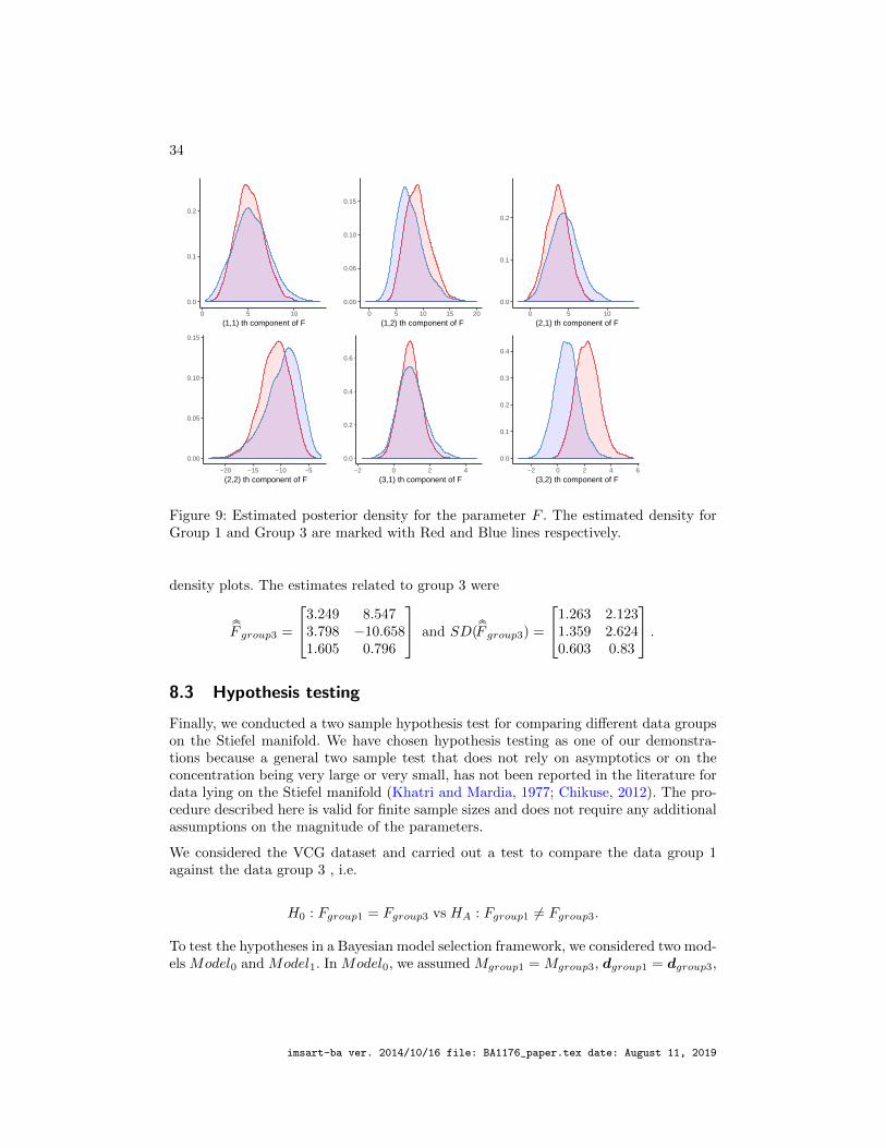