Takustr. 714195 Berlin

GermanyZuse Institute Berlin

JAKOB WITZIG1 AMBROS GLEIXNER2

Conflict-Driven Heuristics for MixedInteger Programming

1 0000-0003-2698-07672 0000-0003-0391-5903

ZIB Report 19-08 (February 2019)

Zuse Institute BerlinTakustr. 714195 BerlinGermany

Telephone: +49 30-84185-0Telefax: +49 30-84185-125

E-mail: bibliothek@zib.deURL: http://www.zib.de

ZIB-Report (Print) ISSN 1438-0064ZIB-Report (Internet) ISSN 2192-7782

Conflict-Driven Heuristics for Mixed Integer

Programming

Jakob Witzig and Ambros Gleixner

Zuse Institute Berlin, Takustr. 7, 14195 Berlin, Germany{witzig,gleixner}@zib.de

February 6, 2019

Abstract

Two essential ingredients of modern mixed-integer programming (MIP)solvers are diving heuristics that simulate a partial depth-first search ina branch-and-bound search tree and conflict analysis of infeasible sub-problems to learn valid constraints. So far, these techniques have mostlybeen studied independently: primal heuristics under the aspect of findinghigh-quality feasible solutions early during the solving process and conflictanalysis for fathoming nodes of the search tree and improving the dualbound. Here, we combine both concepts in two different ways. First,we develop a diving heuristic that targets the generation of valid conflictconstraints from the Farkas dual. We show that in the primal this isequivalent to the optimistic strategy of diving towards the best bound withrespect to the objective function. Secondly, we use information derivedfrom conflict analysis to enhance the search of a diving heuristic akinto classical coefficient diving. The computational performance of bothmethods is evaluated using an implementation in the source-open MIPsolver SCIP. Experiments are carried out on publicly available test setsincluding Miplib 2010 and Cor@l.

1 Introduction

The most commonly used method to solve mixed-integer programs (MIPs) is thelinear programming-based (LP-based) branch-and-bound algorithm (Dakin 1965,Land and Doig 1960). In modern MIP solvers, this procedure is accelerated byvarious extensions (see e.g., Bixby et al. 2000, Laundy et al. 2009). Two examplesof those extensions are primal heuristics (see e.g., Fischetti and Lodi 2010, Lodi2013, Berthold 2014a) and conflict analysis (see e.g., Davey et al. 2002, Sandholmand Shields 2006, Achterberg 2007a, Witzig et al. 2017). A primal heuristic isan incomplete method without any guarantee of success, which is used to findfeasible and improving solutions. Computational studies indicate that within a

1

MIP solver, disabling all primal heuristics would lead to a deterioration of solvingtime by approximately 11% – 32% (Berthold 2014a) and 5% – 15% (Achterbergand Wunderling 2013). Conflict analysis denotes a collection of techniquesto learn from infeasible subproblems encountered during the MIP solve. Theoutcome of conflict analysis is a set of so-called conflict constraints that are usedin the remainder of the solving process, e.g., for propagation. As a consequence,the proof of global optimality can be accelerated, mostly by reducing the numberof subproblems that need to be explored, according to the study of Achterbergand Wunderling (2013) by as much as 28% on affected instances.

In this paper, we propose two complementary ways of combining bothconcepts. Firstly, we develop a primal diving heuristic that explicitly aimsto generate conflict constraints. As we show by elementary calculations, thisamounts to an optimistic fixing of variables to their best bound with respect tothe objective function. Previous approaches that are targeted to gain additionalconflict information starting from a feasible subproblem are based on, for example,an involved random sampling approach (Dickerson and Sandholm 2013) oruse a black-box solver to perform a hybrid constraint programming and MIPsearch (Berthold et al. 2010, 2018). In contrast to that, our approach constitutesa more direct method.

Secondly, we use the information obtained by conflict analysis in order toguide the LP relaxation towards feasibility. To this end, we apply the concept ofvariable locks to conflict constraints and show that this type of locks is richer oninformation and yield a more dynamic criterion compared to variable locks asknown from the literature (Achterberg 2007b). We use this to develop a newdiving heuristic that harnesses variable locks implied by conflict constraints. Ourexperiments indicate that this heuristic outperforms the well-known coefficientdiving heuristic (Berthold 2008).

To show how a MIP solver can benefit from the techniques presented in thispaper as supplementary features, we carry out a detailed computational studyfor which both heuristics were implemented within the academic MIP solverSCIP 6.0 (Gleixner et al. 2018). The heuristics presented in this paper are – tothe best of our knowledge – the first LP-based heuristics for MIP which explicitlyproduce and exploit conflict constraints.

This paper is organized as follows. In Section 2 we give a brief overview of allthe background we need in the remainder of this paper: LP-based branch-and-bound, diving heuristics, and conflict analysis. In Section 3 we discuss how adiving heuristic can be used to generate additional conflict information explicitly.Afterward, we present a modification and extension of the well-known divingheuristic coefficient diving by using conflict information in Section 4. Finally,an intense computational study of the individual impact of both presentedapproaches is presented in Section 5. In Section 6 we conclude.

2

2 Background

We consider MIPs of the form

min{cTx | Ax ≥ b, ` ≤ x ≤ u, xj ∈ Z∀j ∈ I}, (1)

with objective coefficient vector c ∈ Rn, constraint coefficient matrix A ∈ Rm×n,constraint right-hand side b ∈ Rm, and variable bounds `, u ∈ Rn

, whereR := R ∪ {±∞}. Moreover, let I ⊆ N := {1, . . . , n} be the index set of integervariables.

LP-based Branch-and-bound. Branch-and-bound (Dakin 1965, Land andDoig 1960) is a divide-and-conquer method which splits the search space se-quentially into smaller subproblems that are ideally easier to solve. For eachsubproblem a lower bound is computed. To this end, the integrality requirementsare omitted and the LP relaxation

min{cTx | Ax ≥ b, ` ≤ x ≤ u, x ∈ Rn} (2)

is solved. On the other hand, an upper bound on the global problem is given bythe objective value of the incumbent solution, i.e., the best solution found so far,if available.

During the branch-and-bound procedure subproblems are regularly fathomed,either due to bounding or infeasibility. In the first case, subproblems whose lowerbound exceeds the global upper bound are disregarded because they cannotcontain an improving solution. Therefore, it is evident that branch-and-boundalgorithms benefit directly from finding good solutions as early as possible. Thesesolutions either originate directly from the LP relaxation when all variables fulfillthe integrality conditions in the LP solution, or are constructed by so-calledprimal heuristics (Fischetti and Lodi 2010, Lodi 2013, Berthold 2014a). In thesecond case, the infeasibility of a subproblem is either proven by contradictingvariable bound changes or by an infeasible LP relaxation. If a node is fathomeddue to infeasibility modern MIP solvers use conflict analysis (Davey et al. 2002,Achterberg 2007b, Witzig et al. 2017) to “learn” from those subproblems. Notethat every subproblem fathomed due to bounding can be interpreted as aninfeasible subproblem after adding a cutoff constraint on the objective functionthat restricts the feasible region to improving solutions.

Diving Heuristics. A special type of primal heuristics are so-called divingheuristics such as fractional-diving and pseudo-cost diving (Berthold 2008). Theprinciple idea of diving heuristics comes from the branch-and-bound procedureitself. Starting from a feasible but fractional LP solution, diving heuristicsalternate between fixing some integer variables to a rounded value based on afractional LP solution and reoptimizing the LP relaxation. This procedure canbe viewed as a partial tree search along one path from the current subproblemto a leaf. Diving heuristics use a special branching rule that usually tendstowards feasibility. By contrast, branching rules for complete tree search such as

3

Algorithm 1: GenericDivingProcedure

Input : LP solution xLP , rounding function φ, score function ψOutput : Solution candidate x or NULL

1 x← NULL, x← xLP

2 D ← {j ∈ I | xj /∈ Z} // diving candidates

3 while x == NULL and D 6= ∅ do4 forall i ∈ D do

1. Determine rounding direction: dj ← φ(j)

2. Calculate variable score: sj ← ψ(j)

5 Select candidate xj with maximal score sj and current local bounds`j and uj

6 Update D ← D \ j7 if dj == up then `j ← dxje else uj ← bxjc8 (optional) Propagate this bound change9 Update D if propagation fixed some j ∈ D

10 if Infeasibility detected then11 Analyze infeasibility, add conflict constraints, perform 1-level

backtrack12 If D = ∅ goto 20 or 5 otherwise

13 (optional) Solve local LP relaxation14 if Infeasibility detected then15 Analyze infeasibility, add conflict constraints, perform 1-level

backtrack16 If D = ∅ goto 20 or 5 otherwise

17 Update x and D if LP was solved18 if xj ∈ Z for all j ∈ I or D == ∅ then19 x← x

20 return x

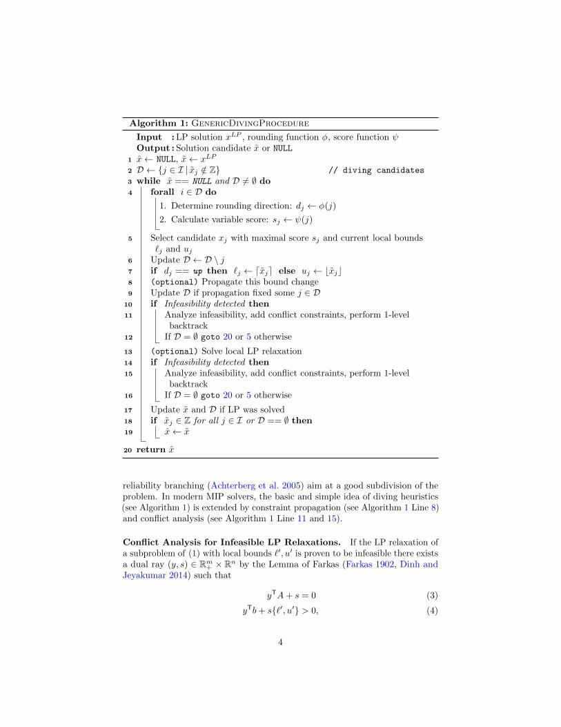
reliability branching (Achterberg et al. 2005) aim at a good subdivision of theproblem. In modern MIP solvers, the basic and simple idea of diving heuristics(see Algorithm 1) is extended by constraint propagation (see Algorithm 1 Line 8)and conflict analysis (see Algorithm 1 Line 11 and 15).

Conflict Analysis for Infeasible LP Relaxations. If the LP relaxation ofa subproblem of (1) with local bounds `′, u′ is proven to be infeasible there existsa dual ray (y, s) ∈ Rm

+ × Rn by the Lemma of Farkas (Farkas 1902, Dinh andJeyakumar 2014) such that

yTA+ s = 0 (3)

yTb+ s{`′, u′} > 0, (4)

4

where we use the notations{`′, u′} :=∑

j∈N : sj>0 sj`′j+

∑j∈N : sj<0 sju

′j . There-

fore, the inequality

(yTA)x ≥ yTb (5)

is globally valid. We refer to (5) also as Farkas proof. Polik (2015) and Witziget al. (2017) describe how these constraints can be collected, managed, and usedfor constraint propagation to deduce tighter variable bounds in modern MIPsolvers.

3 Farkas Diving

Our first aim is the design of a diving procedure such that the dual solutionof the LP relaxation moves towards a valid Farkas proof, i.e., constraints (3)and (4) are satisfied. Suppose x? is an optimal but fractional solution of a localLP relaxation with respect to bounds `′ and u′. Let (y?, r?) be an optimalsolution of the dual LP

max{yTb+ r{`′, u′} | yTA+ r = c, y ∈ Rm+ , r ∈ Rn}, (6)

where rj is the reduced cost of xj , for all j ∈ N . The dual solution (y?, r?) is notfeasible for (3) and (4) with (y, s) = (y?, r?), but note that (y, s) = (y?, r? − c)fulfills (3).

In order to reduce the violation of (4), we need to increase the lower bound`′j of xj if r?j − cj > 0 and decrease the upper bound u′j if r?j − cj < 0. Bycomplementary slackness, all integer variables with fractional LP solution valuehave reduced costs zero, i.e., r?j = 0. Here, without loss of generality we assume`′j , u

′j ∈ Z for all j ∈ I. Hence, tightening the lower or upper bound of variable

j reduces the violation of (4) by |cj | · dj , where

dj :=

{dx?je − `′j if cj < 0,

u′j − bx?jc if cj > 0.(7)

Therefore, the rounding direction of a variable j is implied by the sign of theobjective coefficient cj , i.e., upwards if cj < 0, downwards if cj > 0.

The previous part of this section took a strictly dual point of view. Whenswitching the perspective to the primal side, the above rounding procedure can beinterpreted as follows. On variables with negative objective coefficients we alwaystighten the lower bounds, i.e., the solution values of those variables are pushedtowards the upper bound, and vice versa. Since (1) is a minimization problem,all variables are rounded into the best direction with respect to the objectivefunction c. If cj = 0 neither pushing to the lower nor upper bound has a directimpact on the objective function. In that case, a natural choice for breakingthis tie is to consider the fractionality fj := x?j − bx?jc of the corresponding LPsolution value. This leads to the following diving heuristic, defined by a rounding

5

function φF and scoring function ψF . For every variable j ∈ I, let

φF (j) :=

{up if cj < 0 or cj = 0 ∧ fj ≥ 1

2 ,

down if cj > 0 or cj = 0 ∧ fj < 12 .

(8)

While we use the fractionality only for tie-breaking, other diving heuristics, e.g.,fractionality diving (Achterberg 2007b), use this criterion solely to determiningthe rounding directions.

In addition to the rounding direction φF , an order needs to be defined inwhich the diving candidates are explored. As discussed before, the violation ofthe dual infeasibility constraint (4) can be reduced by |cj | · dj when tighteningthe lower or upper bound of variable j. From the primal point of view, thepotential change in the objective function depends on how much a variable canbe pushed until it reaches one of its bounds. This change can be approximatedby |cj | · frelj , where

frelj :=

{1− fj if φF (j) = up,

fj if φF (j) = down,(9)

is the relative fractionality of x?j , for all j ∈ I. This measure is used by, e.g.,pseudo cost diving (Achterberg 2007b), to define an ordering in which thevariables are explored during diving.

Combining both criteria, let the score of j ∈ I be given by

ψF (j) := |cj | · dj · frelj . (10)

A higher score is preferred.In the following, we refer to this diving heuristic as Farkas diving. Its rounding

procedure pushes all variable towards the so-called pseudo solution (Achterberg2007b). In the pseudo solution, each variable takes the best bound with respectto its objective coefficient as solution value. This relaxation solution is overlyoptimistic and most of the time not feasible for the constraints Ax ≥ b. However,if this strategy leads to a feasible solution, it may be expected to be very good.

4 Conflict Diving

We continue by exploring the complementary question of how conflict constraintscan be used to guide the search of a diving heuristic. First, consider the followingwell-known concept.

Definition 1 (Variable Locks (Achterberg 2007b)). For a mixed integer programof form (1), the number of down-locks and up-locks of variable j ∈ N is definedas the number of positive coefficients per column ζ+

j := |{i | Aij > 0}| and the

number of negative coefficients per column ζ−j := |{i | Aij < 0}|, respectively.

6

Starting at an LP solution x? satisfying Ax ≥ b, a variable j ∈ I with zerodown-locks ζ+

j (with zero up-locks ζ−j ) can always be set to its lower bound(upper bound) without increasing the violation of any constraint. On the otherhand, if a variable has down-locks (up-locks), rounding the variable downwards(upwards) might increase the violation of at least one constraint. If a constraintdown-locks variable j and is tight with respect to the LP solution candidatex?, rounding x?j downwards will violate the constraint. Hence, the variablelocks measure the “risk” that rounding a variable leads to additional constraintviolations.

Usually, only variable locks that are implied by model constraints (short:variable locks) are used during a MIP solve, e.g., during presolving, propagation,or primal heuristics. A well-known diving heuristic that solely relies on variablelocks is coefficient diving (Berthold 2008). coefficient diving as implemented inSCIP follows the diving scheme of Algorithm 1. For every variable the roundingdirection is determined based on the variable locks only. For a variable j that islocked in both directions, i.e., ζ−j > 0 and ζ+

j > 0, coefficient diving prefers thedirection with less variable locks, i.e., the “safe” direction. The order to processthe variables during diving is given by the number of variable locks, too. Here,variables with many variable locks on the chosen direction are preferred.

Processing variables first that tend to lead to infeasibilities is often called afail fast strategy. This strategy was introduced by Haralick and Elliott (1980) inthe context of artificial intelligence and constraint programming. Later, Berthold(2014a) verified that taking the most critical decisions first is a good strategy forMIP.

Variable locks are a very static criterion and include also model constraintsthat either do not propagate frequently or are not tight at the current LPrelaxation. For this reason, we propose to consider also variable locks impliedonly by conflict constraints (short: conflict locks), which can be defined analogousto Definition 1. The following lemma shows that conflict locks can have theeffect of measuring the “risk” more accurately.

Lemma 2. Let (yTA)x ≥ yTb be a Farkas proof derived from an infeasibleLP and (y, r) a dual ray proving the infeasibility of this local subproblem. Ifthe conflict contributes to the conflict up-locks (conflict down-locks) of j, then,there exists at least one model constraint that contributes to the variable up-locks(variable down-locks) of j.

Proof. The coefficient of xj in the conflict constraint (yTA)x ≥ yTb is aj :=∑mk=1 akj · yi. If aj < 0, i.e., the conflict up-locks xj then there must exist

at least one constraint k with akj < 0 because y ≥ 0. Hence, constraint kcontributes to the variable up-locks of xj . The analogous argument holds foraj > 0.

This motivates the use of conflict locks: they measure the “risk” of violatingboth model and conflict constraints but focus on constraints that have beenactively involved in pruning branch-and-bound nodes.

7

A similar concept which is used in SAT is VSIDS (variable state independentdecaying sum) (Moskewicz et al. 2001). The VSIDS score takes the contributionof every variable (and its negated complement) into account. For every variablethe number of clauses (in MIP speaking: conflict constraints) the variable is partof is counted. During continuing the search the VSIDS are periodically scaled bya predefined constant. With this periodically scaling the weight of older clausesis reduced over the time and more recent observation are weighted higher. Incontrast to VSIDS, conflict locks are not periodically scaled and only respectconflict constraints that are part at the current subproblem. This is especiallyinteresting within a MIP solver that uses a pool-based approach to maintain theconflict constraints (Witzig et al. 2017). Therefore, conflict locks give rise to thecurrent set of variables that are involved in conflict constraints, whereas VSIDSalso incorporate past conflict information.

While classical coefficient diving solely relies on variable locks, we exploitLemma 2 and use a combination of both variable and conflict locks. Given aweight κ ∈ [0, 1], the up-weight ρ−j and down-weight ρ+

j of a variable j is given

as a convex combination of both lock types, i.e., ρ−j := κ · ξ−j + (1 − κ) · ζ−jand ρ+

j := κ · ξ+j + (1− κ) · ζ+

j , where ξ−j and ξ+j denote the number of conflict

up-locks and conflict down-locks, respectively.Furthermore, we revert the rounding strategy of coefficient diving: we use

a rounding function preferring the direction that is more likely to lead toinfeasibilities whenever variable j has locks in at most one direction,

φC(j) :=

{up if ρ−j > ρ+

j or ρ−j = ρ+j ∧ fj ≥ 1

2 ,

down if ρ+j > ρ−j or ρ−j = ρ+

j ∧ fj < 12 ,

(11)

Here we may assume that all variables that have no locks at all, i.e., free variables,are already set to their best bound with respect to their objective coefficient.With this strategy we aim to guide the heuristic into parts of the search treethat are usually not explored by other heuristics. The order in which the divingcandidates are explored is identical to the one used in coefficient diving,

ψC(j) :=

{ρ−j if φC(j) = up,

ρ+j if φC(j) = down.

(12)

i.e., variables that have a large number of locks on the chosen rounding directionare preferred. With this scoring function we pursue a fail fast strategy in orderto reduce the time spent by this heuristic. We use a fail fast strategy that iseven more aggressive then coefficient diving since we already choose the criticaldirection. As a result, the heuristic tries to process variables that tend toinfeasibility at the beginning of the diving path before the degree of freedom isfurther reduced during the dive. In the following, we refer to this diving heuristicas conflict diving.

8

5 Computational Results

In order to investigate whether and how MIP solvers can benefit from themethods presented in this paper, we carried out an extensive computationalstudy regarding the individual impact of each heuristic. For each heuristic,we present computational results on its general performance impact, followedby additional experiments that provide more detailed insights regarding theirparticular properties.

In the first part of this section, we compare SCIP in its default configuration(default) to SCIP extended by Farkas diving. We will refer to the latter settingby farkdiving. In the second part of this section, we compare the individualimpact of coefficient diving and conflict diving, to which we will refer by coef-

diving and confdiving, respectively. As a baseline we use SCIP without bothlock-exploiting diving heuristics (nolockdiving).

All experiments were performed with the academic MIP solver SCIP (Gleixneret al. 2018) (git hash bf6a486, based on SCIP 6.0), using SoPlex 4.0 as LPsolver. To evaluate the generated data the interactive performance evaluationtool (IPET) (Hendel) was used. The experiments were run on a cluster ofidentical machines equipped with Intel Xeon E5-2690 CPUs with 2.6 GHz and128 GB of RAM; a time limit of 7200 seconds was set. To account for the effect ofperformance variability (Danna 2008, Lodi and Tramontani 2013) all experimentswere performed with four different global random seeds. As test set we used aunion of Miplib 3 (Bixby et al. 1998), Miplib 2003 (Achterberg et al. 2006),Miplib 2010 (Koch et al. 2011), and the Cor@l (Linderoth and Ralphs 2005)benchmark set. After removing all duplicates and problems that are knownto be numerically unstable, the test set consists of 488 publicly available MIPproblems, which we will refer to as MMMC. Every pair of MIP problem and seedis treated as an individual observation, effectively resulting in a test set of 1952instances. We will use the term “instance” when referring to a problem-seedcombination.

Aggregated results over all random seeds are shown in Table 1 and Table 3.Here, 5 and 11 instances, respectively, are excluded because at least one settingfinished with numerical violations. Besides the results on MMMC, the tablesstate the impact on affected instances, i.e., instances for which the solving pathdiffers among settings. Further, the subset of affected instances is grouped intoa hierarchy of increasingly harder classes [k,tilim]. Class [k,tilim] contains allinstances for which all settings need at least k seconds and can be solved byat least one setting within the time limit. As explained by Achterberg andWunderling (2013), this excludes instances that are “easy” for all settings in anunbiased manner. Detailed tables with instance-wise computational results canbe found in the electronic supplement.

5.1 Farkas Diving

We first present computational experiments regarding the general impact ofFarkas diving as proposed in Section 3. In this setup, Farkas diving solved the

9

Table 1: Aggregated computational results for Farkas diving on MMMC over fourdifferent random seeds. Relative changes by at least 5% are highlighted in bold.

default farkdiving

# S T N Fvirt Ivirt S TQ NQ F I

all 1947 1401 183 3366 2.653 0.806 1408 0.982 0.947 3.725 0.335Miplib 2010 348 305 349 6225 3.454 0.828 307 0.966 0.940 4.862 0.379

affected 706 686 66 1204 4.238 0.564 693 0.946 0.852 5.924 0.585[10,tilim] 529 509 186 2420 5.168 0.733 516 0.918 0.808 6.112 0.573[100,tilim] 297 277 697 4444 6.997 0.980 284 0.852 0.737 6.862 0.690[1000,tilim] 127 107 2599 8072 11.764 1.291 114 0.837 0.715 10.803 1.150afterroot 273 270 34 1095 9.747 0.689 272 0.879 0.783 15.319 1.513

LP relaxation at every diving node (cf. Line 13). Since this strategy is costlycompared to other diving heuristics in SCIP, Farkas diving was executed at localnodes of the search tree, if the heuristic could already find a feasible solution atthe root node. Moreover, since Farkas diving relies on the objective function,we executed the heuristic on instances with a nonzero objective function only.In the second part, we discuss additional computational experiments used toanalyze the effect of the individual components of Farkas diving.

Overall Impact of Farkas Diving. Aggregated computational results com-paring SCIP in its default configuration (default) and SCIP extended by Farkasdiving (farkdiving) on MMMC are shown in Table 1. Due to the restrictedexecution strategy described above, farkdiving affected only 706 out of 1947instances. However, on these 706 instances farkdiving led to a speed-up of5.4 % (TQ) and reduced the tree size by 14.8 % (NQ).

On the subset of harder instances [100,tilim] the overall performance couldeven be improved by 14.8 % and the size of the search tree could be reducedby more than 25 %. The observed performance improvement is spread overthe complete group of affected instances. This becomes apparent also in theperformance profiles (Dolan and More 2002, Gould and Scott 2016) displayed inFigure 1. For a time factor of 1.0 the respective amount of instances that couldbe solved best with the respective setting is marked with a colored cross. In ourexperiments, we observed that on the set of affected instances default performsbest on 369 instances, whereas farkdiving was marginal worse and performsbest on 365 affected instances. On this group of instances, both profiles crossexactly once at time factor 1.021. Afterward, farkdiving is always superior todefault. This fact indicates that farkdiving is especially superior to default

on harder instances and is confirmed by the performance profiles over instanceswhere both settings need at least 10, 100 or 1000 settings. On these groups ofaffected instances, farkdiving is clearly superior to default. For a time factorof 1.0 farkdiving performs best the harder the instances are. On the group ofaffected instances for which both settings need at least 10 seconds 248 can besolved best by default, whereas farkdiving performs best on 281 instances.

10

These results indicate that Farkas diving is expensive on easy instances comparedto default, but superior on harder instances.

Success in Generating Conflicts. Farkas diving is motivated by the idea ofexplicitly diving towards a valid Farkas proof. To analyze how successful Farkasdiving is in generating conflict constraints we considered all affected instanceswhere Farkas diving was allowed to run after the root node, i.e., instanceswhere Farkas diving was able to find a feasible solution at the root node. Thissubset contains 273 instances and is displayed in line “afterroot” of Table 1.On this subset of instances, Farkas diving was able to find 7.3 % more conflictconstraint than the “virtual best diving heuristic” in this regard. Here, thevirtual best diving heuristic is determined by taking, for each instance run withdefault settings, the diving heuristic that generated the largest number ofconflict constraints. Hence, Farkas diving indeed succeeded in generating anabove-average number of conflict constraints. Figure 2 provides a more detailedcomparison of the number of generated conflict constraints for increasingly hardsubgroups of afterroot. The box plots (McGill et al. 1978) show for every settingand instance group the 1st and 3rd quartile (shaded box) as well as the median(dashed line). All observations below the 1st or above the 3rd quartile aremarked with shaded diamonds. On all four groups of instances, Farkas divingled to more conflict constraints in the median and 3rd quartile than the virtualbest diving heuristic in this regard. On instances where both settings neededat least 1000 seconds, Farkas diving produced on 50 % of the instances moreconflict constraints than the virtual best diving heuristic of SCIP with default

settings on 75 % did. These results indicate that the strategy of diving towardsa valid Farkas proof as performed by Farkas diving leads to additional conflictinformation and succeeds over the whole set where this strategy is pursued.Note that our analysis is conservative. The virtual best diving heuristic strictlyoverestimates every single diving heuristic, hence the number of additionallygenerated conflict constraints would only increase when comparing to each divingheuristic individually.

Success in Generating Solution. Usually, the number of solutions foundby diving heuristics is quite small (Khalil et al. 2017). From a primal viewpoint,Farkas diving follows a rounding strategy which leads to overly optimisticsolutions that are expected to be infeasible most of the time. However, if thisstrategy succeeds, the solutions can be expected to be very good. A more detailedlook into the success rate of Farkas diving with respect to finding primal solutionsanswers the question about the impact of these overly optimistic solutions on theoverall MIP solver. In our experiments over several seeds, we could observe thaton affected instances Farkas diving was able to find 39.7 % more feasible solutions(F) and 3.7 % more improving solutions (I) than the virtual best diving heuristic(Fvirt and Ivirt) of SCIP with default settings. Here, the virtual best divingheuristic is determined as above, for each instance selecting the heuristic with thelargest number of feasible and improving solutions, respectively. Again, both F

11

2 4 6 8 100.3

0.4

0.5

0.6

0.7

0.8

0.9

1.0

Time factor

default farkdiving

(a) affected

2 4 6 8 100.3

0.4

0.5

0.6

0.7

0.8

0.9

1.0

Time factor

(b) [10,tilim]

2 4 6 8 100.3

0.4

0.5

0.6

0.7

0.8

0.9

1.0

Time factor

(c) [100,tilim]

2 4 6 8 100.3

0.4

0.5

0.6

0.7

0.8

0.9

1.0

Time factor

(d) [1000,tilim]

Figure 1: Performance profiles of default and farkdiving for four hierarchical groupsof increasingly hard, affected instances.

12

100

1000

10000

Gen

erate

dC

on

flic

ts

default farkdiving

afterroot [10, tilim] [100, tilim] [1000, tilim]0

20

40

60

Instance Group

Figure 2: Box plot showing the number of generated conflicts by Farkas diving whenrunning with farkdiving and the virtual best diving heuristic when running withdefault on increasingly hard subgroups of afterroot.

virt and Ivirt overestimate every single diving heuristic in default setting. Notethat this evaluation is conservative also in the sense that it includes instancesfor which Farkas diving was not allowed to run at local nodes of the tree, i.e.,instances where Farkas diving did not find a solution at the root node, and,therefore, did not find a solution at all in these instances.

On the group of instances where Farkas diving was allowed to run within thetree (afterroot), the results are even more pronounced. Farkas diving was ableto find 57.2 % more feasible solutions and more than twice as many improvingsolutions than the virtual best diving heuristic in default setting. Figure 3 plotsthe relation of feasible and improving solutions found by Farkas diving and thevirtual best diving heuristic of default on increasingly hard groups of afterroot.The box plots show for every setting and instance group the 1st and 3rd quartileof all numbers of feasible and improving solutions, respectively, (shaded box)as well the median (dashed line). All observations below the 1st or above the3rd quartile are marked with shaded diamonds. On all four groups of instances,Farkas diving was able to find 10 or more feasible solution on at least 25 % of theinstances (observations above the 3rd quartile), whereas the 3rd quartile of thevirtual best diving heuristic in this regard is always 1 for affected and [10,tilim].On hard instances for which both setting need at least 1000 seconds the 1stand 3rd quartiles of both default and farkdiving are identical. Note, the setafterroot only contains instances for which Farkas diving was able to find atleast one feasible solution at the root node. Thus, this set of instances is slightlybiased; hence, it is not suitable to conclude that Farkas diving finds more feasiblesolutions than the virtual best diving heuristic in general. However, the resultson this set of instances indicate that the rule we used to decide whether Farkasdiving is allowed to run within the tree succeeds. On the complementary setconsisting of 1562 instances that could be solved by at least one setting, i.e., thosefor which Farkas diving was not able to find a solution root node, farkdivingsucceeded with respect to finding at least one feasible solution within the tree

13

10

100

Fou

nd

Solu

tion

s

default farkdiving

afterroot [10, tilim] [100, tilim] [1000, tilim]0

2

4

6

Instance Group

10

100

Imp

rovin

gS

olu

tion

s

default farkdiving

afterroot [10, tilim] [100, tilim] [1000, tilim]0

1

2

3

Instance Group

Figure 3: Box plots showing the number of feasible and improving solutions foundby Farkas diving when running with farkdiving and the virtual best diving heuristicwhen running with default.

14

Table 2: farkdiving with and without adding feasible solutions and generated conflictconstraints, respectively.

# S T N TQ NQ

default 273 270 33.82 1095 1.000 1.000farkdiving 273 272 29.75 857 0.879 0.783farkdiving-noconfs 273 266 31.79 976 0.940 0.891farkdiving-nosols 273 269 32.73 1045 0.968 0.954

on only 0.019 % of the instances. Considering the improving solutions found bythe virtual best diving heuristic when running SCIP with default settings andFarkas diving indicates that whenever Farkas diving was allowed to run withinthe tree, i.e., it founds a feasible solution at the root node, Farkas diving yieldsat least one improving solution on 75 % (all observations above the 1st quartile)of the instances of afterroot, [10,tilim], and [100,tilim]. By contrast, the 1stand 3rd quartile of the virtual best diving heuristic are 0 and 1, respectively.Consequently, we can conclude that on instances that are cumbersome for theestablished diving heuristics of SCIP 6.0 with respect to finding solutions, Farkasdiving can easily find both feasible and improving solutions if it is allowed torun within the tree.

However, the pure amount of feasible and improving solutions alone is notmeaningful enough to conclude whether the solutions found by Farkas divinghave a positive impact on the overall MIP solver. Therefore, we consider also theprimal integral (Berthold 2013), which measures the progress of the primal boundtowards the optimal solution. Compared to default, farkdiving improvedthe primal integral by 12.3 %. This exhibits, maybe surprisingly so, that theoptimistic strategy of Farkas diving is also very successful on the primal sideand, thus, a valuable extension to the portfolio of primal heuristics.

Impact of Primal Solutions and Generated Conflicts. The previousresults indicate that Farkas diving both produces an over-average number ofsolutions and conflict constraints if it is allowed to run within the tree, but donot finally answer which component is more relevant for performance. We triedto quantify this by testing two modified versions of Farkas diving: one thatdisables conflict analysis (farkdiving-noconfs) and one that discards feasiblesolutions found by Farkas diving (farkdiving-nosols). The aggregated resultsare reported in Table 2. For this experiment, we used the subset of 273 instanceswhere Farkas diving was allowed to be executed after the root node when runningFarkas diving, i.e., afterroot.

Both settings solve fewer instances than default. This result is not surprisingsince both farkdiving-noconfs and farkdiving-nosols spend computationaltime for running Farkas diving. As we have already discussed, Farkas diving ismuch more expensive than other diving heuristics in SCIP since it solves the LPat every node during diving. Consequently, by not performing conflict analysis

15

or not adding feasible solutions during Farkas diving one of the key ingredients ismissing. Thus, on a few instances, Farkas diving needs the impact of both foundsolutions and generated conflict constraints to compensate the computationaloverhead compared to default.

When disabling conflict analysis (farkdiving-noconfs) the performanceimprovement compared to default decreased from 12.1 % to 6 %. The numberof nodes explored during the tree search also increased (compared to fark-

diving) but is still 10.9 % smaller than SCIP with default settings. Disablingthe addition of primal solutions found by Farkas diving to the main search (fark-diving-nosols) reduced the performance improvement compared to default

from 12.1 % to 3.2 %, which corresponds to a slowdown by 9.2 % comparedto farkdiving. Interestingly, the tree increased by 17.9 % compared to fark-

diving. However, farkdiving-nosols still led to 4.6 % smaller trees than SCIP

with default settings.In hindsight, it is not very surprising that disabling the addition of solutions

has a larger impact than disabling conflict analysis during Farkas diving. Withthe very optimistic rounding strategy, Farkas diving was able to find 3.2 timesas many best solutions1 as all remaining diving heuristics together. Overall,on afterroot, 5.7 % of all best solutions were found by Farkas diving. Theonly heuristic that was even more effective on this set of instances is the largeneighborhood search heuristic Rens (Berthold 2014b), which contributed 7.9 %of all best solutions. Thus, Farkas diving has a remarkable success rate, whichleads to a not negligible impact on the primal side. As mentioned above, this isalso reflected by the primal integral (Berthold 2013), which improved by 12.3 %when running Farkas diving during the tree search (afterroot).

These results make clear that both the primal and dual aspects of Farkasdiving contributes to the improved performance, but that the solutions foundwith the strategy of Farkas diving seem to be the main driver of the heuristic.This may come as a surprise because our initial motivation for the design ofFarkas diving was the targeted generation of conflict constraints.

Impact of LP Frequency. By default, all diving heuristics in SCIP areconfigured to solve the LP dependent on the number of found bound deductionsduring constraint propagation over all variables. An LP solve is triggeredwhenever the number of bound changes since the last LP solve exceeds 0.15 timesthe number of variables. By contrast, Farkas diving solves the LP at every divingnode. One motivation for this high LP frequency is to “pull” the variableassignments back towards the feasible region in order to counteract the veryoptimistic rounding strategy of Farkas diving, which tends to “push” the variableassignments out of the feasible region.

Within SCIP, every LP solution found during diving is automatically roundedto a solution satisfying all integrality requirements of the variables. If thissolution also satisfies all constraints, i.e., is feasible for the entire MIP, the

1A solution is called ’best’ if it is an optimal solution or the best-known solution whenreaching the time limit.

16

solution is added to the solution storage, whereby the diving heuristic thatperforms the current dive is credited for finding the feasible solution. Thus,Farkas diving may have a slight advantage over all other diving heuristics sinceit solves the LP relaxation more frequently. This fact might be one reason whyFarkas diving was able to find more than 40 % more solutions than the virtualbest (Fvirt), see Table 1. Hence, in a final control experiment, we configuredFarkas diving identically to all remaining diving heuristics in order to measurethe impact of the increased LP frequency. We will refer to this configuration byfarkdiving-lp.

On the set of affected instances for which our criteria for running Farkasdiving within the tree is satisfied (afterroot), farkdiving-lp performed almostas “poorly” as farkdiving-nosols (see Table 2) with respect to solving time,nodes, and number of solved instances. Thus, when using farkdiving-lp thesolving time could be improved by only 3.5 % compared to default. Note, onthe same set of instances farkdiving led to a speed-up of 12.1 %. Comparedto farkdiving, the amount of feasible solutions found by farkdiving-lp wasreduced by 90 %.

These results show that solving the LP relaxation frequently gives an im-portant boost to the degree by how much Farkas diving improves performance.However, also Farkas diving with less LP solves, i.e., configured identically to allremaining diving heuristics, outperforms the default settings. Consequently,the fact that Farkas diving works indeed seems to be a result of its specific choiceof rounding function φF and scoring function ψF .

5.2 Conflict Diving

The new conflict diving is closely related to the existing coefficient diving inthe sense that they both exploit lock information and follow the same divingframework of Algorithm 1. Hence, we chose to include both in the computationalanalysis and compare their impact individually to SCIP without any of theselock-exploiting diving heuristics. In the following, we will refer to the lattersetting by nolockdiving. We will refer to SCIP with conflict diving and withcoefficient diving activated by confdiving and coefdiving, respectively. Wefirst present computational experiments to quantify the general performanceimpact, followed by further computational results to analyze the impact ofindividual components in more detail.

Overall Impact of Conflict Diving. In our computational setup, conflictdiving used the same parameter settings as coefficient diving, e.g., frequency ofexecution and LP solve frequency. The parameter to weight variable and conflictlocks within conflict diving was set to κ = 0.75, i.e., conflict locks dominate bya factor of 3. Aggregated computational results of all three configurations onMMMC are shown in Table 3.

While coefdiving only showed minimally improved performance comparedto nolockdiving, the setting confdiving was clearly superior. Conflict divingincreased the number of solved instances by 16 (S), led to an overall speed-up

17

Table 3: Aggregated computational results for coefficient and conflict diving on MMMCover four different random seeds. Relative changes by at least 5% are highlighted inbold.

nolockdiving coefdiving confdiving

# S T N S TQ NQ C S TQ NQ C

all 1941 1372 216 3108 1381 0.998 1.003 1386.4 1388 0.978 0.972 1364.4Miplib 2010 347 297 425 5788 299 1.008 1.015 374.9 300 0.986 0.975 343.6

affected 861 822 186 4259 831 0.998 1.014 686.2 838 0.952 0.945 892.2[10,tilim] 775 736 287 5356 745 0.998 1.018 760.9 752 0.948 0.941 990.0[100,tilim] 542 503 707 7982 512 0.988 1.000 1045.2 519 0.932 0.923 1377.9[1000,tilim] 246 207 2365 19538 216 0.984 0.981 2068.5 223 0.874 0.882 2820.5

of 4.8 % (TQ), and reduced the tree size by 5.5 % (NQ) on affected instances.On the subset of affected instances, confdiving needed 4.6 % less solving timeand up to 6.8 % fewer nodes compared to coefdiving. The node reduction onthe affected instances may be explained by the increased number of generatedconflict constraints (C).

Concerning the number of solutions, we observed that confdiving wasonly slightly more successful: confdiving found 11.1 % more feasible solutionsand 4.7 % more improving solutions than coefdiving. The impact of theseadditional solutions is reflected by the primal integral, which decreased by 4.7 %compared to coefdiving and by 4.9 % compared to nolockdiving. However,both heuristics had a small success rate with respect to finding solutions: 0.037(conflict diving) and 0.035 (coefficient diving) solutions per dive.

Finally, the performance profiles in Figure 4 show that the overall performanceimprovement was not caused by few instances but was spread over the completegroup of affected instances: confdiving dominates coefdiving on all fourgroups of increasingly hard instances. For a time factor of 1.0 the respectivepercentage of instances that could be solved fastest with the respective settingis marked with a colored cross. On all four groups of instances, confdivingis clearly superior to coefdiving in the sense that the profiles do not cross.Between 52.0 % and 54.8 % of the instances in the respective group were solvedfastest by confdiving, whereas only between 44.8 % and 46.5 % of the instanceswere solved fastest by default.

Length of Diving Paths. Both the rounding and scoring functions used byconflict diving aim for a fail fast strategy (Haralick and Elliott 1980, Berthold2014a). In order to analyze whether conflict diving indeed achieves this designgoal, we additionally measured the average length of diving paths for coefdivingand confdiving. On average, confdiving exhibits 30.2 % shorter diving pathsthan coefdiving on affected instances.

The distribution of the length of diving paths over the subsets of affectedinstances can be seen in Figure 5. The box plots show for every setting andinstance group the 1st and 3rd quartile of all diving path lengths (shaded box)

18

2 4 6 8 100.3

0.4

0.5

0.6

0.7

0.8

0.9

1.0

Time factor

coefdiving confdiving

(a) affected

2 4 6 8 100.3

0.4

0.5

0.6

0.7

0.8

0.9

1.0

Time factor

(b) [10,tilim]

2 4 6 8 100.3

0.4

0.5

0.6

0.7

0.8

0.9

1.0

Time factor

(c) [100,tilim]

2 4 6 8 100.3

0.4

0.5

0.6

0.7

0.8

0.9

1.0

Time factor

(d) [1000,tilim]

Figure 4: Performance profiles of coefdiving and confdiving for four hierarchicalgroups of increasingly hard affected instances.

19

100

1000

avg.

Dep

th

coefdiving confdiving

affected [10, tilim] [100, tilim] [1000, tilim]0

20

40

Instance Group

Figure 5: Box plots showing the average depth of diving paths generated coefficientdiving with coefdiving and conflict diving with confdiving on the set of affectedinstances.

as well the median (dashed line). All observations below the 1st or above the3rd quartile are marked with shaded diamonds. For all four instance groups, the1st and 3rd quartile corresponding to conflict diving are smaller than for coef-

diving. The same observation holds for the median in all cases. For example,on [100,tilim] the 3rd quartile (149) of coefficient diving is 69.3 % larger thanthe 3rd quartile (87) of conflict diving. On the same group of instances, theobserved median path length of conflict diving is 23.6 % shorter than the one ofcoefficient diving.

As we already discussed, both coefficient diving and conflict diving showedonly a small number of found solutions per diving path, which is a good proxyfor the number of successful paths, i.e., paths without backtracking due toinfeasibility (cf. Line 11 and 15). Thus, these statistics confirm that conflictdiving succeeds better in implementing a fail fast strategy and aborting themany “unsuccessful” dives not leading to a feasible solution early.

Moreover, this does not come at the expense of learning less conflict con-straints. As can be seen in column C of Table 3, confdiving created 30.0 %more conflict constraints.

Impact of Conflict Locks. In order to investigate whether conflict divingoutperforms coefficient diving because of the inclusion of conflict locks or merelybecause of the difference in the rounding and scoring function, we conductedtwo further control experiments with

• a modified rounding function within conflict diving and

• different weights κ.

For the first control experiment we modified conflict diving to use the samerounding function as coefdiving and κ = 0.5 for the scoring function. The

20

resulting diving heuristic conf-like-coefdiving behaves the same as coefficientdiving except for using a convex combination of variable and conflict locks inthe variable selection score.

In our experiment conf-like-coefdiving was superior to coefdiving andled to a performance improvement of 2.3 % on the set of affected instances. Atthe same time, the tree size could be reduced by 3.6 % and four more instancescould be solved. Similar to the actual version of conflict diving evaluated at thebeginning of this section, conflict diving with conf-like-coefdiving settingsgenerated more than twice as many conflict constraints and found 8 % moreimproving solutions than coefficient diving. The performance profiles in Figure 6show that conflict diving with the same rounding function like coefficient divingperforms better the harder the instance, i.e., whenever many conflict constraintsand therefore reliable conflict locks can be expected. It is not surprising that fora time factor of 1.0 coefdiving solves more instances best when easy instancesare considered, too, since the number of conflict constraints can be expected tobe small and, thus, the information gained by conflict locks might not be reliableenough. Even though the profiles are close to each other, they do not cross ifboth settings need at least 10, 100, or 1000 seconds. This result indicates thatit is the inclusion of conflict locks in general that helps to guide diving betterthan pure variable locks.

For the second control experiment we varied the weights κ ∈ {0, 0.25, 0.5, 0.75, 1}in confdiving in order to quantify the importance of conflict locks. The resultsindicate that the reduced length of diving paths is independent of the weightingof variable and conflict locks. For every choice of κ the average length of divingpaths was reduced by 18 % to 34 %. Hence, the length of the diving paths seemsto mainly depend on the rounding function φC , which always prefers roundinginto the “risky” direction, i.e., the direction with more locks. We also confirmedthat confdiving is superior to coefdiving on the affected instances for everyevaluated κ.

Moreover, we observed that on instances with zero objective function asmaller conflict weight κ yields superior performance, while for instances withnonzero objective function a larger weight κ for conflict information seems tobe the better choice. This observation may be related to how and when thedecisions of conflict diving align with SCIP’s default branching rule and whenthey complement it. To make this clear, further background information isnecessary. For branching variable selection, SCIP combines reliability pseudocost-branching (Achterberg et al. 2005), which estimates dual bound improvement,and hybrid branching (Achterberg and Berthold 2009), which includes conflictinformation via VSIDS (Moskewicz et al. 2001). Both VSIDS and conflict locksapproximate the set of variables that frequently appear in conflict constraints.On problems with nonzero objective function typically the first, objective-basedscore dominates SCIP’s branching decisions, while on pure feasibility problemsthe latter, conflict-based score has more impact. This explains that on feasibilityproblems a larger κ might align the decisions of conflict diving unfavorably withthe overall tree search and create redundancy; on the majority of problems withnonzero objective, where conflict information is underweighted in the branching

21

2 4 6 8 100.3

0.4

0.5

0.6

0.7

0.8

0.9

1.0

Time factor

coefdiving conf-like-coefdiving

(a) affected

2 4 6 8 100.3

0.4

0.5

0.6

0.7

0.8

0.9

1.0

Time factor

(b) [10,tilim]

2 4 6 8 100.3

0.4

0.5

0.6

0.7

0.8

0.9

1.0

Time factor

(c) [100,tilim]

2 4 6 8 100.3

0.4

0.5

0.6

0.7

0.8

0.9

1.0

Time factor

(d) [1000,tilim]

Figure 6: Performance profiles of coefdiving and the conflict diving modification conf-

like-coefdiving for four hierarchical groups of increasingly hard affected instances.

22

Table 4: confdiving with and without adding feasible solutions and generated conflictconstraints, respectively, on the set of affected instances.

# S T N TQ NQ

nolockdiving 861 822 185.62 4235 1.000 1.000coefdiving 861 831 185.25 4290 0.998 1.013confdiving 861 838 176.57 3999 0.951 0.944confdiving-noconfs 861 825 181.99 4131 0.980 0.976confdiving-nosols 861 838 177.64 4006 0.957 0.946

rule, a larger κ enables conflict diving to contribute more complementary infor-mation to the search. This suggests a further refinement of conflict diving byadapting the weight κ dynamically to the problem at hand.

Impact of Primal Solutions and Generated Conflicts. Finally, we an-alyzed the importance of found solutions and generated conflict constraintsby comparing confdiving to two artificially modified versions of conflict div-ing: one that does not apply conflict analysis (confdiving-noconfs) and onethat discards feasible solutions found by conflict diving (confdiving-nosols).Aggregated results on the set of affected instances are shown in Table 4.

Both variants confdiving-noconfs and confdiving-nosols are superiorto coefdiving with respect to solving time and number of nodes. Whereasconfdiving-nosols solved the same amount of instances as confdiving, dis-abling conflict analysis led to solving 13 instances less than confdiving. Hence,disabling the addition of feasible solutions found by conflict diving only has amarginal impact compared to standard conflict diving. By contrast, disablingconflict analysis during conflict diving leads to a slowdown of 3 % compared toconfdiving. Thus, the conflict constraints generated during conflict diving seemto be the main driver of the heuristic. This also aligns with our observationsregarding the dual integral (Berthold 2013). The dual integral measures theprogress of the dual bound towards the optimal objective value. This measureincreased by 3.1 % on average when disabling conflict analysis, which indicatesthat the increased number of conflict constraints helps to accelerate convergenceof the proof of optimality.

6 Conclusion

In this paper, we presented two new ways how conflict analysis and primalheuristics can be combined to improve the performance of a MIP solver. Wepresented a primal heuristic, called Farkas diving, that simultaneously aims toconstruct valid Farkas proofs and feasible solutions. By design, Farkas diving ismore expensive than previous diving heuristics in SCIP. Therefore, the heuristicis called conservatively, whereby the decision to keep the heuristic enabled forthe remainder of the search is based on its success during the root node. On the

23

set of instances where Farkas diving was executed after the root node, it provedto be very successful in generating improving solutions and conflict constraints.Regarding both metrics, Farkas diving outperforms the virtual best of all otherdiving heuristics on this set of instances. Moreover, the overall solving timecould be improved by 5.4 % and the tree size could be reduced by 14.8 % on theset of affected instances.

Furthermore, we applied the concept of variable locks to conflict constraintsand used this additional information to guide the search of a second divingheuristic, called conflict diving. In addition, conflict diving pursues an aggressivefail fast strategy to prevent fruitless consumption of running time. This newdiving heuristic is an extension and modification of the well-known coefficientdiving heuristic. Our computational results indicate that this mix of variable andconflict locks in combination with an aggressive fail fast strategy outperformscoefficient diving on our complete test set. Conflict diving reduces the overallsolving time and tree size on affected instances by 4.8 % and 5.5 %, respectively.

The two ways of combining primal heuristics and conflict analysis presentedin this paper have highlighted that primal and dual solving techniques within ageneral-purpose MIP solver are not independent and that they can not only in-teract randomly and create performance variability, but be combined beneficiallyin a targeted manner.

Acknowledgments Many thanks to Timo Berthold for valuable discussionsand Gregor Hendel for his continuous effort in developing IPET. The work forthis article has been conducted within the Research Campus Modal funded by theGerman Federal Ministry of Education and Research (grant number 05M14ZAM)and has received funding from the European Union’s Horizon 2020 researchand innovation programme under grant agreement No 773897 (plan4res). Thecontent of this paper only reflects the author’s views. The European Commission/ Innovation and Networks Executive Agency is not responsible for any use thatmay be made of the information it contains.

References

Achterberg T (2007a) Conflict analysis in mixed integer programming. Discrete Opti-mization 4(1):4–20.

Achterberg T (2007b) Constraint integer programming.

Achterberg T, Berthold T (2009) Hybrid Branching. van Hoeve WJ, Hooker JN,eds., Integration of AI and OR Techniques in Constraint Programming forCombinatorial Optimization Problems, 309–311 (Berlin, Heidelberg: SpringerBerlin Heidelberg), ISBN 978-3-642-01929-6.

Achterberg T, Koch T, Martin A (2005) Branching rules revisited. Operations ResearchLetters 33(1):42–54.

Achterberg T, Koch T, Martin A (2006) MIPLIB 2003. Operations Research Letters34(4):361–372, URL http://dx.doi.org/10.1016/j.orl.2005.07.009.

24

Achterberg T, Wunderling R (2013) Mixed integer programming: Analyzing 12 yearsof progress. Junger M, Reinelt G, eds., Facets of Combinatorial Optimization:Festschrift for Martin Grotschel, 449–481 (Springer Berlin Heidelberg), URLhttp://dx.doi.org/10.1007/978-3-642-38189-8_18.

Berthold T (2008) Heuristics of the Branch-Cut-and-Price-Framework SCIP. KalcsicsJ, Nickel S, eds., Operations Research Proceedings 2007, 31–36.

Berthold T (2013) Measuring the impact of primal heuristics. Operations ResearchLetters 41(6):611–614, URL http://dx.doi.org/10.1016/j.orl.2013.08.007.

Berthold T (2014a) Heuristic algorithms in global MINLP solvers. Ph.D. thesis, URLhttp://www.zib.de/berthold/Berthold2014.pdf.

Berthold T (2014b) RENS. Mathematical Programming Computation 6(1):33–54, ISSN1867-2957, URL http://dx.doi.org/10.1007/s12532-013-0060-9.

Berthold T, Feydy T, Stuckey PJ (2010) Rapid Learning for Binary Programs. Lodi A,Milano M, Toth P, eds., Integration of AI and OR Techniques in Constraint Pro-gramming for Combinatorial Optimization Problems, 51–55 (Berlin, Heidelberg:Springer Berlin Heidelberg), ISBN 978-3-642-13520-0.

Berthold T, Stuckey PJ, Witzig J (2018) Local Rapid Learning for Integer Programs.Technical Report 18-56, ZIB, Takustr. 7, 14195 Berlin.

Bixby ER, Fenelon M, Gu Z, Rothberg E, Wunderling R (2000) MIP: Theory andPractice — Closing the Gap. Powell MJD, Scholtes S, eds., System Modellingand Optimization, 19–49 (Boston, MA: Springer US), ISBN 978-0-387-35514-6.

Bixby RE, Ceria S, McZeal CM, Savelsbergh MWP (1998) An Updated Mixed IntegerProgramming Library: MIPLIB 3.0. Optima 58:12–15.

Dakin RJ (1965) A tree-search algorithm for mixed integer programming problems.The Computer Journal 8(3):250–255.

Danna E (2008) Performance variability in mixed integer programming. Workshop onMixed Integer Programming, Columbia University, New York, volume 20.

Davey B, Boland N, Stuckey PJ (2002) Efficient Intelligent Backtracking Using LinearProgramming. INFORMS Journal of Computing 14(4):373–386.

Dickerson JP, Sandholm T (2013) Throwing darts: Random sampling helps tree searchwhen the number of short certificates is moderate. Sixth Annual Symposium onCombinatorial Search.

Dinh N, Jeyakumar V (2014) Farkas’ lemma: three decades of generalizations formathematical optimization. TOP 22(1):1–22, ISSN 1863-8279, URL http://dx.

doi.org/10.1007/s11750-014-0319-y.

Dolan ED, More JJ (2002) Benchmarking optimization software with performanceprofiles. Mathematical programming 91(2):201–213.

Farkas J (1902) Theorie der einfachen ungleichungen. Journal fur die reine und ange-wandte Mathematik 124:1–27, URL http://eudml.org/doc/149129.

Fischetti M, Lodi A (2010) Heuristics in mixed integer programming. Wiley Encyclopediaof Operations Research and Management Science .

Gleixner A, Bastubbe M, Eifler L, Gally T, Gamrath G, Gottwald RL, Hendel G,Hojny C, Koch T, Lubbecke ME, Maher SJ, Miltenberger M, Muller B, PfetschME, Puchert C, Rehfeldt D, Schlosser F, Schubert C, Serrano F, Shinano Y,Viernickel JM, Walter M, Wegscheider F, Witt JT, Witzig J (2018) The SCIPOptimization Suite 6.0. Technical Report 18-26, ZIB, Takustr. 7, 14195 Berlin.

25

Gould N, Scott J (2016) A note on performance profiles for benchmarking software.ACM Transactions on Mathematical Software (TOMS) 43(2):15.

Haralick RM, Elliott GL (1980) Increasing tree search efficiency for constraint satisfac-tion problems. Artificial intelligence 14(3):263–313.

Hendel G (????) IPET interactive performance evaluation tools. https://github.com/GregorCH/ipet.

Khalil EB, Dilkina B, Nemhauser GL, Ahmed S, Shao Y (2017) Learning to RunHeuristics in Tree Search. Proceedings of the 26th International Joint Conferenceon Artificial Intelligence, 659–666, IJCAI’17 (AAAI Press).

Koch T, Achterberg T, Andersen E, Bastert O, Berthold T, Bixby RE, Danna E,Gamrath G, Gleixner AM, Heinz S, Lodi A, Mittelmann H, Ralphs T, SalvagninD, Steffy DE, Wolter K (2011) MIPLIB 2010. Mathematical Programming Com-putation 3(2):103–163, URL http://dx.doi.org/10.1007/s12532-011-0025-9.

Land AH, Doig AG (1960) An Automatic Method of Solving Discrete ProgrammingProblems. Econometrica 28(3):497–520.

Laundy R, Perregaard M, Tavares G, Tipi H, Vazacopoulos A (2009) Solving HardMixed-Integer Programming Problems with Xpress-MP: A MIPLIB 2003 CaseStudy. INFORMS Journal on Computing 21(2):304–313, URL http://dx.doi.

org/10.1287/ijoc.1080.0293.

Linderoth JT, Ralphs TK (2005) Noncommercial software for mixed-integer linearprogramming. Integer programming: theory and practice 3:253–303.

Lodi A (2013) The heuristic (dark) side of MIP solvers. Hybrid metaheuristics, 273–284(Springer).

Lodi A, Tramontani A (2013) Performance variability in mixed-integer programming.Theory Driven by Influential Applications, 1–12 (INFORMS).

McGill R, Tukey JW, Larsen WA (1978) Variations of box plots. The AmericanStatistician 32(1):12–16.

Moskewicz MW, Madigan CF, Zhao Y, Zhang L, Malik S (2001) Chaff: Engineeringan efficient SAT solver. Proceedings of the 38th annual Design AutomationConference, 530–535 (ACM).

Polik I (2015) Some more ways to use dual information in MILP. InternationalSymposium on Mathematical Programming (Pittsburgh, PA).

Sandholm T, Shields R (2006) Nogood learning for mixed integer programming. Work-shop on Hybrid Methods and Branching Rules in Combinatorial Optimization,Montreal.

Witzig J, Berthold T, Heinz S (2017) Experiments with Conflict Analysis in MixedInteger Programming. Salvagnin D, Lombardi M, eds., Integration of AI and ORTechniques in Constraint Programming, 211–220 (Cham: Springer InternationalPublishing), ISBN 978-3-319-59776-8.

26