Conformal Geometry of Simplicial Surfaces(ROUGH DRAFT)

Keenan Crane

Last updated: March 9, 2019

This document is a referee draft of course notes from the AMS Short Course onDiscrete Differential Geometry in January, 2018. It is under review for the AMSProceedings of Symposia in Applied Mathematics.

1

CONTENTS

1 Conformal Geometry of Simplicial Surfaces 31.1 Overview . . . . . . . . . . . . . . . . . . . . . . . . . . . . . . . . . . . 31.2 Preliminaries . . . . . . . . . . . . . . . . . . . . . . . . . . . . . . . . . 71.3 Part I: Discretized Conformal Maps . . . . . . . . . . . . . . . . . . . . 10

1.3.1 Interior Angle Preservation . . . . . . . . . . . . . . . . . . . . 111.3.2 Cauchy-Riemann Equation . . . . . . . . . . . . . . . . . . . . 121.3.3 Critical Points of Dirichlet Energy . . . . . . . . . . . . . . . . 141.3.4 Hodge Duality . . . . . . . . . . . . . . . . . . . . . . . . . . . 151.3.5 Conjugate Harmonic Functions . . . . . . . . . . . . . . . . . . 16

1.4 Part II: Circle Preservation . . . . . . . . . . . . . . . . . . . . . . . . . 191.4.1 Circle Packings . . . . . . . . . . . . . . . . . . . . . . . . . . . 201.4.2 Circle Patterns . . . . . . . . . . . . . . . . . . . . . . . . . . . . 211.4.3 Discrete Ricci Flow . . . . . . . . . . . . . . . . . . . . . . . . . 24

1.5 Part III: Metric Scaling . . . . . . . . . . . . . . . . . . . . . . . . . . . 261.5.1 Conformally Equivalent Discrete Metrics . . . . . . . . . . . . 261.5.2 Intrinsic Delaunay Triangulations . . . . . . . . . . . . . . . . 291.5.3 Discrete Uniformization . . . . . . . . . . . . . . . . . . . . . . 31

1.6 Part IV: Hyperbolic Polyhedra . . . . . . . . . . . . . . . . . . . . . . . 341.6.1 Hyperbolic Geometry . . . . . . . . . . . . . . . . . . . . . . . 341.6.2 Ideal Hyperbolic Polyhedra . . . . . . . . . . . . . . . . . . . . 361.6.3 Variational Principles . . . . . . . . . . . . . . . . . . . . . . . 381.6.4 Variational Principle for Discrete Uniformization . . . . . . . 43

1.7 Summary . . . . . . . . . . . . . . . . . . . . . . . . . . . . . . . . . . . 45

2

1 CONFORMAL GEOMETRY OF SIMPLICIAL SURFACES

Keenan Crane

1.1 Overview

What information about a surface is encoded by an-gles, but not lengths? This question encapsulates thebasic viewpoint of conformal geometry, which studiesholomorphic or (loosely speaking) angle- and orientation-preserving maps between manifolds. In the discretesetting, however, the idea of literally preserving an-gles leads to an interpretation of conformal geometrythat is far too rigid: the space of discrete solutionslooks far more restricted than the space of smooth so-lutions it hopes to model. Instead, one must considerhow several equivalent points of view in the smoothsetting lead to a number of inequivalent treatmentsof conformal geometry in the discrete setting. Thisactivity has recently culminated in a complete discreteuniformization theorem for polyhedral surfaces, whichbeautifully mirrors the classic uniformization theorem for Riemann surfaces.

Why study discrete conformal geometry? From an analytic point of view, smoothconformal maps provide a strong notion of regularity, since they are complex ana-lytic and hence have derivatives of all orders. In the discrete setting one thereforeobtains one possible notion of what it means for a discrete (e.g., simpicial) map tobe “regular,” even though no derivatives are available in the classical sense. Froma topological point of view, conformal maps help one define canonical mappingsbetween spaces—for instance, uniformization provides an explicit map betweenany two conformally equivalent surfaces, by passing through a canonical domain ofconstant curvature. Likewise, discrete conformal geometry can be used as a startingpoint for constructing canonical maps between simplicial surfaces, even when theydo not have compatible triangulations [39, 2]. In applications, discrete conformalgeometry has become a powerful tool for digital geometry processing algorithms,since many tasks ultimately boil down to solving sparse linear systems or easy con-vex optimization problems. Discrete conformal maps have hence become essentialfor tasks ranging from regular surface remeshing [16], to machine learning [57], todigital fabrication [50, 72]. Discrete conformal geometry also arises in the context of

3

statistical mechanics, where theories based on discrete harmonic functions [75] andcircle patterns [54, 48] appear to be quite natural.

Discretization of conformal maps is an excellent example of “The Game” playedin discrete differential geometry [24], since there are a large number of different(yet equivalent) characterizations of conformal maps in the smooth setting, eachof which leads to a distinct starting point for a discrete definition. Consider forinstance a smooth, nondegenerate, and orientation-preserving map f from a disk-like surface M with Riemannian metric g to the flat complex plane C. A reasonablycomprehensive list of ways to assert that f is conformal includes:

1. (ANGLES) Preservation of angles—at every point p 2 M the angle betweenany two tangent vectors X, Y 2 Tp M is the same as the angle between theirimages dfp(X), dfp(Y) in the plane.

2. (CIRCLES) Preservation of circles—the image of any geodesic circle of radius# approaches a Euclidean circle as # goes to zero.

3. (ANALYTIC) The map f satisfies the Cauchy-Riemann equation—df (JX) =ıdf (X) for all vector fields X, where ı is the complex unit and Jp : Tp M ! Tp Mis the linear complex structure expressing a rotation by p/2 in each tangentspace (J 2

p = �id).

4. (METRIC) Conformal equivalence of metrics—the metric g on M is relatedto the induced metric g := df ⌦ df via a positive scaling g = e2ug, whereu : M ! R>0 is called the log conformal factor.

5. (CONJUGATE) Conjugate harmonic functions—the map f can be expressedas f = a + bı, where a, b : M ! R are harmonic functions with orthogonalgradients of equal magnitude (rb = Jra).

6. (DIRICHLET) Critical points of Dirichlet energy—among all homeomorphismsfrom M to f (M), the map f is a critical point of the Dirichlet energy ED( f ) :=R

M |df |2 dA, where dA is the area measure on (M, g).

7. (HODGE) Hodge duality—the Hodge star on differential 1-forms induced byf is the same as the pushforward under f of the 1-form Hodge star on theoriginal domain.

To someone familiar with smooth conformal geometry this list may seem redundant,since in most cases cases the conceptual leap between one characterization andanother is very small. Yet these minor shifts in perspective often lead to substantiallydifferent interpretations in the discrete setting. In almost all cases, the “discretesetting” means we are considering a domain M encoded as either

4

1. a triangulated surface, or

2. a quadrilateral net.

These notes focus primarily on triangulations; see [4] and references therein for anoverview of the quadrilateral case. Our aim is to give a broad overview of some ofthe highlights of discrete conformal geometry; many details have therefore beenomitted (though see the bibliography for a detailed list of references). The notes areorganized into four parts:

• Part I explores how a naïve treatment of discretization (e.g., preservation ofangles in the triangulation, or direct discretization of the Cauchy-Riemannequation) leads to definitions of discrete conformal maps that are excessivelyrigid, or agree with the smooth theory only in the limit of refinement.

• Part II shows the first glimpse of real “discrete” theories based on preserva-tion of circles (circle packings and circle patterns). This perspective capturesmany important features of conformal geometry, and very nearly provides acomplete theory of discrete uniformization for general triangulations.

• Part III considers the perspective of conformally equivalent discrete metrics;this is to date the most satisfactory theory of conformal maps for triangulatedsurfaces, since it comes with a complete uniformization theorem.

• Part IV makes the connection between discrete conformal mapping prob-lems and realization problems for ideal hyperbolic polyhedra, which alsoilluminates the relationship between theories based on circles (Part II) andconformally equivalent metrics (Part III).

Importantly, the focus in these notes on structure preservation should not beconfused with a value judgement on utility: numerical schemes that do not ex-actly capture smooth structure may nonetheless be perfectly suitable for practicalcomputation (especially on fine tessellations), and are often less computationallydemanding than those that furnish an exact discrete theory. The same trade off canbe found throughout discrete differential geometry: exact structure preservationoften comes at significant computational cost relative to cheaper numerical alter-natives. A negative interpretation is that one is therefore stuck between fast butinexact numerical schemes, and those that are “exact” but slow. A more maturepoint of view is that the two sets of tools are complementary: fast numerical meth-ods help to initialize or approximate intermediate computations needed for exact,structure-preserving schemes, which in turn provide valuable guarantees about thebehavior of algorithms. Beyond computation, discrete conformal geometry helps to

5

bridge several areas of mathematics, including some rather remarkable connectionsbetween geometry, analysis, and combinatorics, as well as Euclidean and hyperbolicgeometry. It also highlights a central thesis of discrete differential geometry, namelythat the most important features of geometry are not inherently smooth nor discrete,but (as we will see) can be faithfully described in either language.

6

1.2 Preliminaries

Throughout we consider a compact connected surface M with Riemannian metric g.In Part I we will mainly consider a differentiable map f from a disk-like domainM to the complex plane C (with its usual Euclidean metric); this setup allowsus to focus on the local picture, and avoid issues of global topology or complexstructure. As discussed in Sec. 1.1, there are many equivalent ways to express that fis conformal; we therefore refrain from choosing a canonical definition, and insteaddiscuss each characterization in turn. The differential dfp : Tp ! Tf (p)C of the mapf expresses how tangent vectors on M are pushed forward to C. We will generallyassume that f is an immersion, meaning that its differential df is nondegenerate, i.e.,at each point p 2 M, d fp(X) = 0 if and only if X = 0. In particular, every conformalmap is an immersion, whereas holomorphic maps can have isolated points wherethe differential fails to be injective. Finally, the linear complex structure associatedwith a surface (M, g) is a tangent space automorphism J : TM ! TM such thatin each tangent space Tp M, (i) J2

p = �id (where id denotes the identity map), and(ii) gp(X,JpX) = 0; intuitively, J defines a quarter-rotation in each tangent spacecompatible with the metric g (in analogy with the imaginary unit ı in the complexplane), and is hence determined by the metric up to a global choice of orientation.

Figure 1: Topologically, we consider surfaces ob-tained by gluing triangles along edges. A toruswith one vertex (top), cone with two vertices(middle), and sphere with three vertices (bottom)can each be expressed as a D-complex, but not asa simplicial complex.

In the discrete setting, we considersurfaces that can be obtained by gluingtogether Euclidean triangles—the proto-typical example is a Euclidean polyhe-dron (such as the icosahedron), thoughwe need not restrict ourselves to surfacesembedded in Rn. Usually it will be suf-ficient to consider simplicial complexes,though for the general theory of discreteconformal equivalence (Part III) we mustconsider more general triangulations—here it will be sufficient to work withD-complexes, as defined by Hatcher [41,Section 2.1]. Fig. 1 gives several exam-ples of triangulations that are not simpli-cial but are expressible as D-complexes.Throughout, we will use the term discretesurface to mean a topological 2-manifoldtriangulated by either a simplicial or D-complex M = (V,E,F), where V, E, andF denote the vertices (0-cells), edges (1-cells), and faces (2-cells), resp. We will usea (k + 1)-tuple of vertex indices to specify

7

a k-simplex; for instance, ij is an edge with vertices i, j 2 V and ijk is a face with ver-tices i, j, k 2 V. (This convention is an abuse of notation in the case of a D-complex,but the meaning will nonetheless be clear.) If a discrete surface has finitely manytriangles, we say that it is finite (and hence compact). The star St(i) of a vertex i 2 Vis the subcomplex of M comprised of all simplices that contain i.

The intrinsic geometry of a discrete surface M = (V,E,F) can be expressed via adiscrete metric, i.e., an assignment of positive edge lengths ` : E ! R>0 that strictlysatisfy the triangle inequality in each face:

`ij + `jk > `ki 8 ijk 2 F.

These edge lengths naturally define a piecewise Euclidean metric on M, obtainedby constructing disjoint Euclidean triangles with the prescribed lengths and gluingthem along shared edges. The resulting space has a singular Riemannian metricg that is Euclidean away from vertices, and “cone-like” in a small neighborhoodaround each vertex i 2 V. Any such metric g is called a (polyhedral) cone metric; amore formal definition is given by Troyanov [84, p. 4].

Figure 2: A cone metric is flat away from isolatedcone points i 2 V, where it looks like a wedge ofpaper (possibly multiply-covered) identified alongthe two marked edges. The angle deficit or excess Widetermines the curvature.

Any discrete metric determines in-terior angles q

jki at each vertex i of

each triangle ijk (e.g., via the law ofsines). Letting

Qi := Âijk2F

qjki

be the total angle around vertex i, thecone angle

Wi := 2p � Qi (1)

measures how close the vertex is tobeing Euclidean, providing a discreteanalogue for Gaussian curvature. In-tuitively, the intrinsic geometry lookslike a circular Euclidean cone, or moregenerally, a circular wedge of the Eu-clidean plane glued together at op-posite edges (Fig. 2). Likewise, forany vertex i on the domain boundary,the angle ki := p �Âijk2F q

jki provides

a discrete analogue for geodesic cur-vature. Together, W and k satisfy a discrete Gauss-Bonnet theorem: Âi Wi2M +Âi2∂M ki = 2pc(M), where c(M) := |V|� |E|+ |F| is the Euler characteristic of M.

8

Figure 3: A discrete branch point, where a piece-wise linear map fails to be a discrete immersion.

For an embedded surface, the extrinsicgeometry can be expressed as a piece-wise linear (or more properly, simplex-wise affine) map interpolating givenvertex coordinates f : V ! Rn. Anysuch map is a discrete immersion if it islocally injective, or equivalently, if foreach vertex i 2 V the restriction of f toSt(i) is embedded [17, Lemma 2.2]. Thecondition that f be a (discrete) immer-

sion not only excludes vanishing angles, zero-length edges, and zero-area triangles,but also avoids discrete branch points (see Fig. 3). It would therefore be reasonableto require any definition of a discrete conformal map to include the condition that fis a discrete immersion; a discrete holomorphic map should likewise be noninjectiveonly at vertices. Any discrete immersion f induces a corresponding discrete metric

`ij := | f j � fi|

(where | · | denotes the Euclidean norm); note that unlike the smooth setting thismetric is nondegenerate even in the presence of branch points.

Since conformal maps depend only on the intrinsicgeometry of a surface, it is important to appreciate thatthe edges of a polyhedron are completely superficial—even when the metric arises from an embedding in Rn.For instance, consider an embedded polyhedron withtwo triangles ijk, jil sharing an edge ij. Since this trianglepair is isometric to a Euclidean quadrilateral (with twopossible diagonals), an intrinsic observer walking alongthe surface has no way to know when they are crossingthe extrinsic edge. Likewise, two discrete surfaces with different triangulations andsets of edge lengths may nonetheless be isometric—consider for instance splittingthe square faces of a cube along different diagonals. From this point of view, theintrinsic geometry of a discrete surface is completely determined by the number ofvertices, along with their locations and cone angles. This situation motivates theconstruction of intrinsic Delaunay triangulations (Sec. 1.5.2), which play an importantrole in the theory of discrete uniformization (Sec. 1.5.3).

9

1.3 Part I: Discretized Conformal Maps

Figure 4: A vertex of a polyhedron (left) is intrinsicallythe same as a circular cone (right), and hence experiencesinfinite scale distortion u when conformally flattened inthe classical sense. (Black lines depict pullback of integergrid lines under a conformal flattening.)

In Part I we consider several can-didate ways to discretize confor-mal maps f : (M, g) ! C froma disk-like domain (M, g) to thecomplex plane C, each of whichfails to capture the behavior ofsmooth conformal maps in someessential way. The first questionto ask, perhaps, is: why do weneed a new definition at all? Af-ter all, a “discrete” surface is stilla Riemannian manifold, and weshould therefore be able to ap-ply standard definitions directly(perhaps with some extra care inorder to deal with cone points).This viewpoint of conformallyequivalent cone metrics has infact been studied by Troyanov [84], though for our purposes it is not the rightphilosophical starting point: it views a polyhedron as a literal description of thegeometry we want to represent, rather than a proxy for a smooth surface. Fromthe classical Riemannian point of view a convex polyhedron does not look muchlike a smooth surface: it is flat almost everywhere, except at a discrete collection ofpoints where it locally looks like a cone. As depicted in Fig. 4, a conformal flatteningof such a metric hence looks nothing like a flattening of a smooth surface, since ithas unbounded scale distortion u in the vicinity of each vertex. We are thereforemotivated to seek an alternative definition for discrete conformal maps, which morefaithfully captures the behavior we expect from smooth surfaces.

The notions studied in this part all begin with a fairly naive hypothesis (e.g.,“discrete conformal maps should preserve angles”), which in each case leads to a definitionthat is significantly more rigid than the smooth definition. An important exceptionis the finite element treatment discussed in Sec. 1.3.5, which provides the expecteddegree of flexibility, but otherwise does not capture many of the basic features ofsmooth conformal maps in an exact sense—for instance, even just composing agiven finite element solution with a Möbius transformation may yield a map thatis not the solution to any finite element problem. In all other cases, one can stillconsider maps which come as close as possible to satisfying the naïve definition,e.g., in the “least-squares” sense—until fairly recently, this point of view has beenthe starting point for most practical computational algorithms [53, 73].

10

1.3.1 Interior Angle Preservation

We first consider the most basic geometric characterization on conformal maps,namely that they should preserve angles. In the smooth setting, an immersionf : M ! C is conformal if at every point p 2 M the angle between any two tangentvectors X, Y 2 Tp M is the same as the angle between their images dfp(X), dfp(Y) inthe plane. A very tempting idea, then, is to seek a discrete immersion f : M ! C

that preserves the interior angles qjki at every triangle corner. However, it quickly

becomes clear that this notion of conformal equivalence is far too rigid: interiorangles are preserved if and only if each triangle ijk 2 F experiences a similaritytransformation, or (intrinsically) if the new and old edge lengths in each triangleijk are related by a scale factor lijk > 0, i.e., ˜ab = lijk`ab for ab 2 ijk. At first glancethis idea of locally scaling the discrete metric in each triangle feels reminiscent ofthe scaling relationship g = e2ug between conformally equivalent smooth metricsg, g. However, since each interior edge ij is shared by two triangles ijk, jil, the scalefactors lijk, ljil of any two adjacent triangles must be identical. Globally, then, anypiecewise linear map that preserves all interior angles is necessarily an isometry,up to a uniform scaling by some constant factor c 2 R>0. Hence, an angle-baseddefinition of conformal equivalence is far too rigid: each equivalence class is aone-parameter family of discrete metrics, parameterized by a single constant c. Instark contrast, smooth equivalence classes are parameterized by a scalar function,namely the log conformal factor u : M ! R. (Yet as we will see in Part III a differentnotion of metric scaling will ultimately lead to the right notion of discrete conformalequivalence.)

Figure 5: Angles thatexhibit Euclidean sumsaround triangles andvertices may still fail tocharacterize a valid tri-angulation.

One can nonetheless consider the map that distorts anglesthe least, i.e., the one that minimizes the deviation of anglesfrom their original values in the least-squares sense [74]. To doso, suppose we parameterize piecewise linear maps f : M ! C

via the interior angles qjki > 0 of the image f(M). These angles

describe a valid planar triangulation as long as they satisfy acollection of discrete integrability conditions:

1. For each triangle ijk 2 F, qjki + qki

j + qijk = p.

2. For each interior vertex i 2 V, Âijk2St(i) qjki = 2p.

3. For each interior vertex i 2 V, ’ijk2St(i)sin qki

j

sin qijk= 1.

The first condition is the usual Euclidean triangle postulate; the second is simply therequirement that every vertex have a Euclidean angle sum. As illustrated in Fig. 5,

11

the third condition is a necessary closure condition on edge lengths around eachvertex, obtained by applying the law of sines to the relationship

’ij2St(i)

˜i,j˜i,j+1

= 1,

where ˜i,j and ˜i,j+1 denote the lengths of consecutive edges in St(i) with respect tocounter-clockwise ordering. The best approximation of an angle-preserving map (inthe least-squares sense) is then any minimizer of the energy

Eang(q) := Âijk2F

(q jki � q

jki )

2,

subject to the condition that the new angles q are positive and satisfy the discreteintegrability conditions outlined above. These angles determine a discrete metric(up to a global uniform scaling), which in turn determines a discrete map to theplane (up to Euclidean motions). Here again we observe too much rigidity inthe sense that Eang typically has only a single unique minimizer (up to Euclideanmotions), whereas in the smooth setting there is a large family of conformal mapsfrom any disk-like domain to the plane. However, this minimizer will at least be adiscrete immersion (due to condition (2) and the positive angle condition), and willexhibit variable rather than uniform scaling. Further properties of such maps arenot well-understood—empirically, for instance, the minimizer of Eang appears toapproximate the conformal map of least area distortion, though this observation hasnever been carefully analyzed. A variety of numerical algorithms for computingsuch maps have been developed [74, 73, 91].

1.3.2 Cauchy-Riemann Equation

Figure 6: Geometrically, the Cauchy-Riemann equation asks that pushing for-ward vectors via given map f commuteswith scaling and rotation.

Analytically, smooth conformal maps on a do-main U ⇢ C are traditionally characterized bythe Cauchy-Riemann equation, which says thata map f : U ! C; (x, y) 7! u(x, y) + ıv(x, y)is holomorphic if

∂u∂x

=∂v∂y

and∂u∂y

= � ∂v∂x

. (2)

If f is also an immersion (i.e., f has a nonvan-ishing derivative), then it is conformal. On reg-ular quadrilateral nets, where one has clear “x”and “y” directions, this coordinate description

12

is a natural starting point for structure-preserving discretizations of holomorphicmaps that capture much of the rich structure found in complex analysis [4]. Forgeneral triangulated surfaces, where there are no clearly distinguished coordinatedirections, one must take a different approach. An alternative way to write Eqn. 2 is

df (ıX) = ıdf (X),

where ı denotes the imaginary unit and X is any tangent vector field on U. In otherwords, a complex map f is holomorphic if pushing forward vectors commuteswith 90-degree rotation. For a surface M with linear complex structure J , a mapf : M ! C is likewise holomorphic if

df (JX) = ıdf (X) (3)

for all tangent vector fields X on M.

When applied to piecewise linear maps f : M ! C, this characterization againleads to a definition for discrete conformal maps that is far too rigid. In particular,the only affine maps that satisfy Cauchy-Riemann on a single triangle are Euclideanmotions and uniform scaling. We therefore encounter the exact same situation aswe did for angle preservation in Sec. 1.3.1: in order for affine maps to agree acrossshared edges, they must all exhibit identical scaling. Hence, a piecewise linear mapf is holomorphic in the sense of Eqn. 3 if and only if it is a global isometry, up to aglobal uniform dilation.

As with angle preservation, one can nonetheless seek the piecewise linear mapf : V ! C that best agrees with the Cauchy-Riemann equation. Consider for instancethe energy

EC( f ) :=Z

M| ⇤ df � ıdf |2 dA, (4)

which measures the L2 residual of Eqn. 3; here, ⇤ denotes the Hodge star operator ondifferential 1-forms. To avoid the trivial solution f = 0, one typically incorporatesa pair of point constraints f (a) = 0, f (b) = 1 (for a, b 2 M, a 6= b). Minimizingthis energy over piecewise linear maps f leads to a standard Galerkin finite elementmethod, yielding a corresponding discrete energy EC(f) (see [23, Chapter 7] fora detailed derivation); this approach was one of the earliest starting points forpractical conformal surface parameterization [53]. As with Eang, the (constrained)discrete energy EC typically has a unique minimizer. In contrast, the smooth energyEC has an enormous space of minimizers—consider composing any minimizer fwith an in-plane conformal map h : f (M) ! C. Hence, the unique minimizerchosen by EC will depend in an unstable way on superficial features of the problem(such as the choice of tessellation), hinting at some of the practical difficulties withdefinitions that are “too rigid”. For further discussion, see [60, Section 3] and [70,Section 2].

13

1.3.3 Critical Points of Dirichlet Energy

The Dirichlet energy of a differentiable map f : M1 ! M2 between Riemannianmanifolds (M1, g1) and (M2, g2) is the functional

ED( f ) :=Z

M1

|df |2 dV,

where dV is the volume measure on M1; f is harmonic if it is a critical point ofED. Purely topological conditions determine whether a harmonic map is alsoholomorphic:

Theorem 1 (Eells & Wood 1975). If f : M1 ! M2 is a harmonic map and

c(M1) + |deg( f )c(M2)| > 0,

then f is either holomorphic or antiholomorphic (where c(M) is the Euler characteristic ofM, and deg( f ) is the topological degree of f ).

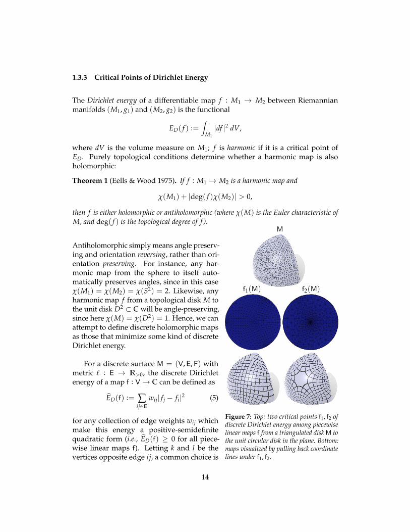
Figure 7: Top: two critical points f1, f2 ofdiscrete Dirichlet energy among piecewiselinear maps f from a triangulated disk M tothe unit circular disk in the plane. Bottom:maps visualized by pulling back coordinatelines under f1, f2.

Antiholomorphic simply means angle preserv-ing and orientation reversing, rather than ori-entation preserving. For instance, any har-monic map from the sphere to itself auto-matically preserves angles, since in this casec(M1) = c(M2) = c(S2) = 2. Likewise, anyharmonic map f from a topological disk M tothe unit disk D2 ⇢ C will be angle-preserving,since here c(M) = c(D2) = 1. Hence, we canattempt to define discrete holomorphic mapsas those that minimize some kind of discreteDirichlet energy.

For a discrete surface M = (V,E,F) withmetric ` : E ! R>0, the discrete Dirichletenergy of a map f : V ! C can be defined as

bED(f) := Âij2E

wij| f j � fi|2 (5)

for any collection of edge weights wij whichmake this energy a positive-semidefinitequadratic form (i.e., bED(f) � 0 for all piece-wise linear maps f). Letting k and l be thevertices opposite edge ij, a common choice is

14

the cotangent weights wij := 12 (cot q

ijk + cot q

jil ), which arise from the finite element

discretization mentioned in Sec. 1.3.2. (Other choices are also possible—see forinstance [40].) A discrete holomorphic map to a fixed region U ⇢ C can then bedefined as a critical point of bED, subject to the condition that boundary vertices aremapped to ∂U; this map will look conformal (rather than just holomorphic) if theboundary polygon has a unit turning number—see Fig. 7 for two examples. Thispoint of view was originally considered by Hutchinson [43]; see also [62].

A closely related point of view is that, in the smooth setting, the conformalenergy EC( f ) of any map f : M ! C can be expressed as the difference between theDirichlet energy ED( f ) and the signed area A( f ) of the image f (M), i.e.,

EC( f ) = ED( f )�A( f )

(see [23, Chapter 7]). In the case where the target is fixed (e.g., if one considersonly maps to the unit disk), the area term A is constant, and hence ED will havethe same minimizers as EC. One can hence define a discrete conformal map f as aminimizer of the discrete Dirichlet energy bED (Eqn. 5) minus the signed area of thetarget polygon (subject to the same point constraints as in Sec. 1.3.2), giving anotherquadratic form in f:

bA(f) := 12 Â

ij2∂M

fi ⇥ fj;

here ∂M denotes the collection of oriented edges in the boundary of M, and z1 ⇥z2 := Im(z1z2). This formulation is used as the starting point for several practicalalgorithms in digital geometry processing [27, 60]. It turns out, however, that theenergy bED � bA is identical to the energy EC obtained by discretizing the Cauchy-Riemann equations [19]. Its minimizers therefore exhibit the same degree of rigidityas before.

1.3.4 Hodge Duality

Figure 8: The ratio of dual overprimal edge length is equal to halfthe sum of the cotangents of theopposite angles q

ijk , q

jil .

Consider the Hodge star ⇤ on differential 1-formsa, which on a smooth surface with linear complexstructure J can be expressed via the relationship1

⇤a(X) = a(JX)

for all tangent vector fields X. Since conformal mapspreserve the linear complex structure, they also pre-serve the 1-form Hodge star. In the discrete setting,

1Note that some authors adopt an opposite orientation convention, i.e., ⇤a(X) = �a(JX).

15

one can reverse this relationship and try to define adiscrete conformal map as one that preserves the (discrete) Hodge star [58]. In partic-ular, differential forms can be discretized as cohains on a simplicial manifold and itspolyhedral dual [88, 26]. A fairly common discretization of the Hodge star is then a“diagonal” linear map from primal k-cochains to dual (n � k)-cochains determinedby the ratio of primal and dual volumes. In the particular case of discrete 1-formson a triangulated surface and its circumcentric dual, a discrete differential 1-formcan be encoded via a value aij per primal edge, and the corresponding (Hodge) dual1-form can be expressed as a value on each dual edge via the cotangent formula:

⇤ aij := 12 (cot q

ijk + cot q

jil )| {z }

wij

aij, (6)

where qijk , q

jil are the angles opposite ij, as depicted in Fig. 8. A discrete conformal

map in the sense of Hodge duality is then any piecewise linear map for which thenew angles q satisfy cot q

ijk + cot q

jil = 2wij, or, from an intrinsic point of view, any

new assignment of edge lengths ˜ij that preserves this same quantity.

Initially, one might be optimistic that a discretization based on the Hodge staryields less rigidity than one based on preservation of angles, since (at least naïvely)preservation of the edge weights wij effectively places only |E| ⇡ 3|V| conditions onthe map f , whereas preservation of interior angles q

jki corresponds to 3|F| ⇡ 6|V|

constraints. However, recent analysis [92, 33] extinguishes any such optimism:

Theorem 2. The primal-dual length ratios wij := 12 (cot aij + cot bij) on a given discrete

surface M = (V,E,F) uniquely determine the discrete metric ` : E ! R, up to globalscaling.

The proof relies on the fact that a metric exhibiting a prescribed Hodge star canbe obtained as a minimizer of a convex function, where the Hessian at any suchminimizer has a kernel consisting only of vectors corresponding to global scalingof `—exactly the same degree of rigidity as with angle preservation (Sec. 1.3.1),Cauchy-Riemann (Sec. 1.3.2), and Dirichlet energy (Sec. 1.3.3).

1.3.5 Conjugate Harmonic Functions

Suppose we express a holomorphic map f : M ! C as f = a + bı for a pair ofreal-valued functions a, b : M ! R. A straightforward consequence of the Cauchy-Riemann equation (Sec. 1.3.2) is that a and b form a conjugate harmonic pair, i.e., they

16

are real harmonic functions with orthogonal gradients:

Da = 0,Db = 0,rb = Jra,

(7)

Here D is the Laplace-Beltrami operator on M, r is the gradient operator, and J isthe linear complex structure.

The conditions in Eqn. 7 are of course closely related to (in fact, equivalent to) thecondition that the map itself be a critical point of Dirichlet energy (Sec. 1.3.3), but theperspective of conjugate harmonic pairs will provide a different starting point fordiscretization, where boundary conditions play a key role. Characterizing conformalmaps in terms of harmonic functions is also attractive from the perspective ofdiscretization, since discrete harmonic functions are well-studied. In the simplicialsetting, a discrete harmonic function f : V ! R is naturally defined as a piecewiselinear function in the kernel of a discrete Laplace-Beltrami operator L : V ! V suchas the cotan Laplacian

(Lf)i := 12 Â

ij2E(cot q

ijk + cot q

jil )(fj � fi). (8)

(See [87] for a more thorough discussion.) To define a conjugate harmonic pair, onethen just needs a discrete notion of conjugacy.

Figure 9: One possible notionof discrete conjugacy: a func-tion on primal (black) vertices isconjugate to a function on dual(white) vertices if the differenceacross primal edges is equal tothe difference across dual edges,up to a constant factor that ac-counts for triangle shape.

What does it mean for two discrete harmonic func-tions to be conjugate? One idea, studied by Mercat andothers [58], is to consider functions on the combinato-rial or Poincaré dual of a discrete surface M = (V,E,F),which associates each vertex with a 2-cell, each edgewith a 1-cell, and each triangle with a 0-cell. In this set-ting, two real-valued functions a, b on the primal anddual 0-cells (resp.) are discretely conjugate if for eachedge e and corresponding dual edge e⇤, the differenceof a values across e is equal to the difference of b valuesacross e⇤, up to a scale factor we 2 R that accountsfor the geometry of the triangulation (as discussed inSec. 1.3.4). In other words, if

bj⇤ � bi⇤ = wij(aj � ai)

for all edges ij 2 E, where i⇤, j⇤ are the associated dual vertices (see Fig. 9). In termsof (discrete) differential forms, we are simply requiring that db = ⇤da, capturingthe conjugacy condition rb = Jra. Here one encounters two basic sources of

17

difficulty. First, as detailed in Sec. 1.3.4, if one views the conformal structure ofa discrete surface as being determined by the edge weights wij (or discrete Hodgestar), then one encounters severe rigidity: the weights uniquely determine a discretemetric. Moreover, pairs of functions a, b that are conjugate in this sense do notdefine a simplicial mapping from M to C, since the coordinates b are associated with0-cells of the dual complex, rather than vertices of the original discrete surface M.

Alternatively, one can take the following approach: given a discrete harmonicfunction a (i.e., a piecewise linear function satisfying La = 0), its harmonic conjugatecan be defined as the function b : V ! R that minimizes the L2 difference betweenJra and rb over the space of piecewise linear functions—or equivalently, whichminimizes the discrete conformal energy bEC(f) = bED(f)� bA(f) of a map f = a+ bı(Sec. 1.3.3), while keeping a fixed. The minimizer is the solution to the discreteLaplace equation Lb = 0 with discrete Neumann boundary data

hi =12(ai+1 � ai�1),

where i � 1, i, and i + 1 denote consecutive vertices along the bound-ary (see [70, Section 4.3.3] for more detail). The resulting mapf := a + bı is then discrete conformal in the same finite elementsense discussed in Sec. 1.3.2. Importantly, however, one finally ob-tains exactly the right amount of flexibility: whereas a “least squares”conformal map [53] of the kind discussed in Sec. 1.3.2 is determinedup to Euclidean motions, one now obtains a whole family of discreteconformal maps f parameterized by the harmonic function a. Sincethis function is in turn determined by its own boundary values, one ends up inprecisely the same situation as in the smooth setting, where holomorphic mapsf : M ! C can be parameterized by real functions on ∂M specifying either Dirichletor Neumann boundary conditions. A more geometric view is that one can param-eterize such maps by specifying either the log conformal factor u or the geodesiccurvature k along the boundary—Sawhney & Crane [70] outline a complete strategyin the piecewise linear setting.

Ultimately, it should come as no surprise that a proper finite element treatmentshould faithfully capture the behavior of smooth conformal maps in the limit ofrefinement. On the other hand, for any fixed triangulation, such maps do not exactlypreserve many basic properties from the smooth setting, such as covariance withrespect to Möbius transformations. Moreover, they do not provide a natural notionof equivalence—for instance, the composition of two piecewise linear harmonicfunctions is not in general harmonic. We will therefore continue in Parts II and III toseek a precise notion of discrete conformal equivalence for finite triangulations.

18

1.4 Part II: Circle Preservation

Figure 10: Left: a smooth Riemann mapping from a simply connected region in the plane to the unitcircular disk. Right: a discrete Riemann mapping, expressed as a circle packing.

A linear map preserves angles if and only if it is the composition of a rotationand a dilation (no shear); hence, it also preserves circles. Since at each point p 2 Mthe differential dfp of a conformal map f is an angle-preserving linear map, itmust also preserve infinitesimal circles. This point of view is the starting point forseveral distinct but closely-related approaches to discrete conformal maps, based onarrangements of circles with special combinatorial and geometric relationships.

Finite arrangements of circles provide fertile soil for discrete conformal maps,capturing many features of the smooth theory. Koebe originally showed howincidence relationships in planar graphs can be captured via tangency relationshipsbetween circles, providing a basic connection between combinatorics and geometry.Thurston conjectured (and Rodin & Sullivan later proved) that these circle packingshave a deep connection to Riemann mappings in the complex plane (Sec. 1.4.1); suchconnections have since been studied intensively by Schramm [69] and many others.To generalize this construction to curved surfaces and irregular triangulations onemust incorporate additional geometric information, such as intersection angles orother data describing relationships between circles; such arrangements fall underthe general heading of circle patterns2 (Sec. 1.4.2).

There are however some missing features, most notably the lack of a uniformiza-tion theorem that guarantees the existence of a constant curvature circle patternequivalent to any given triangulation. In Part III we will see a discrete uniformiza-tion theorem which guarantees existence by considering variable rather than fixedtriangulations; whether one can take an analogous approach in the circle patternsetting remains to be seen. Note that circle packings and patterns have been studied

2There is some inconsistency in the use of packings versus patterns throughout the literature—forclarity we adopt the convention that packings are arrangements of circles meeting tangentially, whereaspatterns describe any arrangement of circles (possibly overlapping or disjoint), whether associatedwith vertices, faces, etc.

19

extensively beyond the context of triangulations and discrete conformal maps; seefor instance [80, 8, 6, 86].

1.4.1 Circle Packings

A circle packing is a collection of closed circular disks in the plane (or other surface)that intersect only at points of tangency—see [79] for an excellent overview. Toany such collection one can associate a graph G = (V,E) (called the nerve) whereeach vertex corresponds to a disk, and two vertices are connected by an edge if andonly if their associated disks are tangent. A natural question to ask is: which graphsadmit circle packings?

Theorem 3 (Circle Packing). Every planar graph G = (V,E) can be realized as a circlepacking in the plane.

(For nonplanar graphs, one can also consider circle packings on surfaces ofhigher genus.) A first hint that circle packings are connected to discrete conformalmaps comes via the following theorem:

Theorem 4 (Koebe). If G is a connected maximal planar graph, then it has a unique circlepacking up to Möbius transformations and reflections.

(A constructive algorithm for computing such packings was given by Collins &Stephenson [21].) A graph is maximal if the addition of any edge makes it nonplanar.If G is also finite, one quickly sees that it is equivalent to a triangulation of thesphere, via stereographic projection. Koebe’s theorem therefore says that any trian-gulated sphere can be realized as a family of planar circle packings parameterizedby Möbius transformations, just as smooth conformal maps from the sphere to theplane have Möbius symmetry. An even richer connection between circle packingsand conformal maps can be made via the Riemann mapping theorem:

Theorem 5 (Riemann mapping). Any nonempty simply connected open set W ( C canbe mapped to the interior of the unit circular disk D2 := {z 2 C : |z| < 1} by a bijectivemap f : W ! D2 that is holomorphic (hence conformal) in both directions.

The circle packing analogue of Riemann mapping was originally conjecturedby Thurston, and later proved by Rodin and Sullivan [68]. The basic idea is to startwith a regular hexagonal circle packing C of a simply connected region W by disksof radius # > 0, i.e., for any hexagonal tiling of the plane, take only those disksthat intersect W. Now find a circle packing C0 that maintains the same incidence

20

relationships, but where all disks along the boundary are now tangent to the unitcircular disk D2 (this idea is illustrated in Fig. 10, right). The relationship betweenthese two packings defines an approximate mapping of W to D2: for sufficiently small# any point z 2 W will be contained in a circle c from C, and can be mapped tothe center of the corresponding circle c0 from C0. Rodin and Sullivan show that theapproximate mapping converges to a conformal homeomorphism as # �! 0.

Figure 11: Discrete surfaces with identicalcombinatorics but different edge lengths (top)yield the same class of circle packings into theunit disk (bottom).

Unlike smooth Riemann mappings, how-ever, one cannot directly use circle packingsto define discrete conformal maps betweenany two disk-like regions, since finite hexag-onal packings of these regions will not ingeneral have the same combinatorics. Moreimportantly, this theory does not provide ageneral approach to uniformization, since itcannot account for the curvature of the do-main, nor triangulations with nonuniformedge lengths. Consider for instance sim-plicial disks with identical combinatoricsbut different discrete metrics ` : E ! R>0,as depicted in Fig. 11. Since a circle pack-ing depends purely on the combinatoricsof the edge graph, these surfaces are real-ized by identical families of circle packings—implying that all discrete metrics on a givensimplicial disk are, effectively, conformallyequivalent. In this sense, the basic theory ofcircle packings is too flexible; one is thereforeprompted to enrich it with additional data.

1.4.2 Circle Patterns

A more direct way to encode the geometry of thedomain is to incorporate additional metric infor-mation into the arrangement of circles. Supposewe associate each edge ij 2 E of a triangulationM = (V,E,F) with an angle wij 2 [0, p

2 ]; the pair(M, w) is called a weighted triangulation. If we nowassign a radius ri > 0 to each vertex i 2 V, thena pair of circles in the Euclidean plane with theprescribed intersection angle wij and radii ri, rj will

21

have centers separated by a distance

`ij =q

r2i + r2

j + 2rirj cos wij. (9)

The condition w p/2 ensures that these lengths satisfy the triangle inequality ineach face ijk 2 F (see [82, Lemma 13.7.2]); they hence determine a discrete metricon the surface (called the circle packing metric), and in turn, a corresponding coneangle Wi at each vertex (Eqn. 1). We can make an analogy between each of thesequantities and data from the smooth setting:

• the edge lengths `ij encode the metric,

• the cone angles Wi encode the Gaussian curvature,

• the intersection angles wij capture the conformal structure, and

• the radii ri (or more precisely, any subsequent changes to the radii) play therole of conformal scale factors.

The last two items on this list can be understood by considering that (i) angles areconformal invariants, and (ii) adjusting the radii (scale factors) will scale the edgelengths ` (metric) while keeping the angles w (conformal structure) fixed. From thispoint of view, finding a conformal map from a curved surface (W 6= 0) to a flat one(Wi = 0 at all vertices) amounts to finding an appropriate adjustment of radii, i.e.,finding the conformal scale factors that flatten the metric. Note however that it isnot immediately clear that a target angle defect W can always be achieved—and ingeneral it cannot. In particular, we have the following theorems [82]:

Theorem 6 (rigidity of circle patterns). For a closed weighted triangulation (M, w), anassignment of cone angles Wi to vertices uniquely determines a unique discrete metric `ij ifone exists—in other words, if there are radii ri at vertices such that (i) circles intersect atthe prescribed angles w and (ii) the edge lengths determined by Eqn. 9 induce the prescribedcone angles W, then this circle pattern is unique up to a uniform scaling of all circle radii /edge lengths.

Theorem 7 (existence of circle patterns). Let M = (V,E,F) be a closed weighted trian-gulation with weights w, and for any subset of vertices I ⇢ V let Lk(I) and FI denote thesimplicial link of I and the set of faces with vertices in I, resp. Then prescribed cone anglesWi can be achieved if and only if

Âi2I

Wi + Âij2Lk(I)

(p � wij) > 2pc(FI),

where c denotes the Euler characteristic.

22

In short: one cannot prescribe curvature arbitrarily, but if the prescribed curva-ture can be achieved, then it uniquely determines the metric (up to global scaling).The condition in Theorem 7 is akin to Gauss-Bonnet, but much stronger: just as anymetric can be uniformized in the smooth setting, one would like the existence ofdiscrete uniformization to depend only on a basic Gauss-Bonnet condition on thecurvature data W, and not on the data w describing the domain itself.

Generalizations. Generalizations of thecircle patterns described above providegreater flexibility. One such generalization,first studied by Bowers and Stephenson [10],is an inversive distance circle packing—herewe exchange the angles wij for values Iij 2[�1, •), and define the edge lengths via theinversive distance

`ij =q

r2i + r2

j + 2rirj Iij.

When Iij = 1 circles are tangent, when Iij < 1 they intersect at an angle wij =arccos(Iij), and when Iij > 1 they are disjoint. In this setting one again has localand global rigidity theorems akin to Theorem 6 [37, 56, 90], though no guarantee ofexistence due to conditions like the one from Theorem 7.

One can also associate a circle pattern with the faces of a triangulation, ratherthan its vertices. Let (M, w) be a weighted triangulation where (i) the weights wijsum to 2p around each interior vertex, and (ii) the values ki := 2p � Âij wij sum to2p over all boundary vertices. One can then find a Euclidean circle pattern withone circle per face, so long as there is a collection of interior angles a

jki that satisfy

Rivin’s coherent angle system [65], namely

1. (Positivity) ajki > 0 at each triangle corner.

2. (Triangle Postulate) ajki + aki

j + aijk = p for each face ijk.

3. (Compatibility) p � wij is equal to aijk + a

jil for each interior edge ij, and equal

to aijk for each boundary edge ij.

For instance, if wij are the intersection angles of the tri-angle circumcircles in a planar Delaunay triangulation, thenthe circle pattern will reproduce this triangulation, up toa global similarity. Existence and uniqueness (up to simi-larity) can be obtained through variational arguments [8].However, this construction does not directly address the

23

task of uniformization, since for a curved domain the in-tersection angles wij will not in general sum to 2p aroundinterior vertices. A practical approach to conformal flatten-ing via facewise circle patterns was proposed by Kharevych et al. [49], who firstconstruct a collection of interior angles a that (i) satisfy Rivin’s conditions, and(ii) approximate the interior angles q

jki of the curved domain in the least-squares

sense. This particular treatment does not however provide a clean notion of discreteconformal equivalence for general (i.e., non-flat) discrete surfaces.

Other generalizations, such as hyper-ideal circle patterns [71, 78], finally providethe right degree of flexibility. In this setting, one associates circles with both verticesand edges—and obtains a discrete uniformization theorem in the case of surfaceswith non-positive curvature [5], even with fixed combinatorics. Such results suggestthat it is not unreasonable to expect a complete discrete uniformization theorembased on patterns of circles (namely, one that includes the positively curved case),though at present it would seem that perhaps the ending has not yet been written.

1.4.3 Discrete Ricci Flow

In the smooth setting, one approach to uniformization is to consider Hamilton’sRicci flow [38], which for surfaces can be expressed as

ddt

g = �Kg.

Here K denotes the Gaussian curvature of the current metric g. Intuitively, Ricciflow shrinks the metric where curvature is “too positive,” and expands it wherecurvature is “too negative,” ultimately smoothing out all bumps in curvature. Sincethe flow applies a pointwise rescaling at each moment in time, the final, uniformizedmetric is conformally equivalent to the initial one. Often one considers a normalizedversion of this flow

ddt

g = (K � K)g

where K is the average Gaussian curvature over the domain; this flow becomesstationary when the metric has constant curvature.

Chow and Luo [18] consider a discrete analogue of this flow based on weightedtriangulations (with intersection angles wij 2 [0, p

2 ])—in particular, they define the(normalized) combinatorial Ricci flow

ddt

ri = (W � Wi)ri,

24

where the values Wi are the cone angles of the circle packing metric determined byri, and W is the average cone angle. If one considers the effect of the radii r on thediscrete metric `, this flow has the same basic behavior as Ricci flow: the metric isrescaled in order to smooth out bumps in curvature. Chow and Luo show that thisflow is defined for all time and converges to a constant curvature metric if one exists,i.e., the flow does not uniformize all initial metrics—the condition on existence isthe same as the one given in Theorem 7. Nonetheless, the flow behaves well enoughin practice to provide a starting point for a wide variety of algorithms in geometriccomputing [35]. Circle patterns can also be connected with other geometric flowssuch as Calabi flow [29, 94], though again Thurston’s condition (Theorem 7) must ofcourse hold in order to guarantee existence of a uniformized circle packing metric.

Luo also considered a closely related combinatorial Yamabe flow [55], defined interms of a different discrete analogue of conformal maps (i.e., one that is not basedon circle packings or patterns). This flow provides a starting point for the notion ofdiscrete conformal equivalence that we will study in Part III, and ultimately, to acomplete discrete uniformization theorem where existence can be guaranteed.

25

1.5 Part III: Metric Scaling

In the smooth setting, two Riemannian metrics g, g on a surface M are conformallyequivalent if they are related by a positive scaling, i.e., if g = e2ug for some functionu : M ! R called the log conformal factor. Hence, eu gives the length scaling, and e2u

is the area scaling. A conformal structure on M is then an equivalence class of metrics.

This section examines a definition for conformal equivalence of discrete metricsthat resembles the one found in the smooth setting, and which ultimately allows oneto formulate a discrete uniformization theorem for polyhedral surfaces (Sec. 1.5.3)that mirrors the one for smooth Riemann surfaces. From an applied point of viewdiscrete uniformization provides a principled starting point for tasks like regularsurface remeshing [16] and constructing maps between polyhedral surfaces [39].We begin with a basic picture involving only Euclidean geometry (Sec. 1.5.1), andwill revisit this story through the lens of hyperbolic geometry in Part IV.

1.5.1 Conformally Equivalent Discrete Metrics

Recall that a discrete metric is an assignment of edge lengths ` : E ! R>0 that satisfythe triangle inequality in each face, i.e., `ij + `jk � `ki for all ijk 2 F. What doesit mean for two discrete metrics `, ˜ to be conformally equivalent? One idea is tosimply mimic the smooth definition and ask that ˜ij = lij`ij for some scale factorlij on each edge ij 2 E. However, this constraint is clearly “too flexible,” since thenevery pair of discrete metrics is conformally equivalent—simply let lij be the ratio˜ij/`ij. Also recall from Sec. 1.3.1 that a scale factor per face is “too rigid,” since one isthen forced to make all scale factors equal. An alternative is to consider scale factorsat vertices [67, 55]:

Definition 1. Two discrete metrics `, ˜ on the same triangulation M = (V,E,F) arediscretely conformally equivalent if for each edge ij 2 E,

˜ij = e(ui+uj)/2`ij, (10)

for some collection of values u : V ! R.

This definition again gives the impression of merely aping the smooth relationship—yet in this case the resulting theory is neither too rigid nor too flexible. Instead, itprovides a rich notion of discrete conformal equivalence that beautifully preservesmuch of the structure found in the smooth setting [7, 36], a perspective which hashad a significant impact on (and has been inspired by) algorithms from digitalgeometry processing [77, 3, 16].

26

One elementary observation is that, locally, conformally equivalent discretemetrics in the sense of Eqn. 10 are still very flexible:

Lemma 1. Any two discrete metrics `, ˜ on a single triangle ijk are discretely conformallyequivalent.

Proof. The metrics are conformally equivalent if there exists an assignment of logscale factors ui, uj, uk to the three vertices such that

e(ua+ub)/2 = ˜ab/`ab

for each edge ab 2 ijk. Let lij := 2 log(`ij) (and similarly for ˜). Then by taking thelogarithm of the system above we obtain a linear system for the u values, namely

ua + ub = lab � lab, 8ab 2 ijk.

This system has a unique solution, independent of the values of ` and ˜. In particular,

eui =˜ij

`ij

`jk˜jk

˜ki`ki

, (11)

and similarly for uj, uk.

Figure 12: A piecewise linearmap is discrete conformal if andonly if it preserves the lengthcross ratio cij := `il`jk/`ki`l jfor each interior edge ij.

At this point it might be tempting to believe thatall discrete metrics are conformally equivalent, sincethey are equivalent on individual triangles. However,since scale factors (at vertices) are shared by severaltriangles, one still obtains an appropriate degree ofrigidity. In particular, an important observation is thatall metrics within the same discrete conformal equiva-lence class can be identified with a canonical collectionof length cross ratios [77]:

Definition. Let ` : E ! R>0 be a discrete metric ona triangulated surface M = (V,E,F). For any pair oftriangles ijk, jil 2 F sharing a common edge ij 2 E, theassociated length cross ratio is the quantity

cij :=`il`jk

`ki`l j. (12)

Theorem 8. Two discrete metrics `, ˜ on the same triangulation M are discretely conformallyequivalent if and only if they induce the same length cross ratios c, c.

27

Proof. First suppose that `, ˜ are discretely conformally equivalent, i.e., that ˜ij =

e(ui+uj)/2`ij for some collection of log conformal factors ui : V ! R. Then

cijkl =˜il ˜jk˜ki ˜l j

=e(ui+ul)/2e(uj+uk)/2`il`jk

e(uk+ui)/2e(ul+uj)/2`ki`l j=

`il`jk

`ki`l j= cijkl .

Now suppose that `, ˜ induce identical cross ratios, i.e., c = c. By Lemma 1, thesemetrics already satisfy the conformal equivalence relation on individual triangles.In particular, for any pair of adjacent triangles ijk, jil, we can find compatible logscale factors ui, uj, uk and vj, vi, vl . Moreover, these scale factors will agree on theshared edge ij if and only if ui = vi and uj = vj. Applying Eqn. 11 we discover thatthis compatibility condition is equivalent to

`jk˜jk

˜ki`ki

=˜il`il

`l j˜l j

,

i.e., equality of cross ratios.

The length cross ratios c : E ! R effectively specify a point in the Teichmüllerspace of discrete metrics; see [7, Remark 2.1.2] for further discussion. Extrinsically,it is not hard to show that for a discrete surface immersed in Rn, length cross ratioswill be preserved by Möbius transformations of the vertices (assuming that thetransformed vertices are connected by straight segments rather than circular arcs).As in the smooth setting, however, the space of maps f : V ! C that induce adiscretely conformally equivalent metric ˜ij := |fj � fi| is much larger than just thespace of Möbius transformations. One characterization is that discrete conformalmaps (in this sense) correspond to piecewise projective maps that preserve trianglecircumcircles [77, Section 3.4]. Connections between conformally equivalent discretemetrics and piecewise Möbius transformations have also been studied [85].

Two elementary examples help reinforce the connection between smooth anddiscrete conformal equivalence:

Example 1 (discrete metrics on the two-triangle sphere). In the smooth setting,all 2-spheres have the same conformal structure. Consider the triangulation ofthe 2-sphere by two triangles depicted in Fig. 1, bottom. Any discrete metric onthis triangulation is determined by three edge lengths `ij, `jk, `ki > 0 satisfying thetriangle inequality. By the same argument as in Lemma 1, all discrete metrics onthis triangulation of the sphere are discretely conformally equivalent—mirroringthe situation in the smooth setting.

Example 2 (discrete metrics on the two-triangle torus). In the smooth setting, thereis a two-parameter family of conformal structures on the torus. Consider the

28

triangulation of the torus depicted in Fig. 1, top. Any discrete metric on thistriangulation is determined by three edge lengths a, b, c corresponding to the edgemarked with a single arrow, the edge marked with a double arrow, and the diagonal.Since there is only one vertex in the triangulation (and hence one scale factor), twosuch metrics are discretely conformally equivalent if and only if they are related bya uniform scaling—partitioning the three-parameter family of discrete metrics intoa two-parameter family of conformal classes (as in the smooth setting).

There are however major difficulties with the theory discussed so far: it onlyallows us to discuss conformal equivalence of polyhedra with identical combina-torics, since it depends on comparing values associated with edges—at this point,for instance, it is not even possible to say that two different triangulations of thecube (with square faces split along different diagonals) are discretely conformallyequivalent, even though they are isometric in the usual sense. Moreover, proceduresfor uniformizing a given discrete metric (discussed in Sec. 1.5.3) may break downbefore achieving constant curvature, i.e., the metric may degenerate into a collectionof edge lengths where the triangle inequality no longer holds. In order to developa full theory of discrete uniformization, we therefore have to understand what itmeans for two combinatorially inequivalent polyhedra to be conformally equivalent.For this, we first need to consider a structure called the intrinsic Delaunay triangula-tion, which enables us to associate a canonical triangulation with any polyhedralcone metric.

1.5.2 Intrinsic Delaunay Triangulations

Delaunay triangulations arise naturally throughout discrete and computational geom-etry, and have numerous characterizations. For a triangulation in the plane, the mosttypical characterization is that the circumcenter of every triangle is “empty,” i.e., novertices of the triangulation are contained in its interior. An equivalent condition isthat the sum of angles opposite every interior edge must be no greater than pi, i.e.,for any two triangles ijk, jil sharing an edge jil,

qijk + q

jil p. (13)

Unlike the empty circumcircle definition, the angle sum condition generalizes in astraightforward way to any triangulated surface M = (V,E,F) with discrete metric` : E ! R>0, since interior angles q are determined (via the law of sines) by theedge lengths `. Any discrete surface (M, `) satisfying Eqn. 13 at each edge is calledintrinsic Delaunay.

29

Figure 14: Left: an edge is Delaunay if the sum of oppositeangles a, b is no greater than p; “flipping” a non-Delaunayedge always yields a Delaunay configuration. Right: theangle sum condition holds with equality if and only if twotriangles are cocircular.

Every polyhedral cone met-ric admits a Delaunay triangu-lation, i.e., given a surface Mwith cone metric g, there al-ways exists at least one triangu-lation of the cone points (ver-tices) where all edges satisfyEqn. 13 [45]. In an extrinsicsetting, one can imagine that agiven polyhedron in R3 is trian-gulated by different collectionsof geodesic arcs terminating atvertices—not necessarily corre-sponding to the extrinsic edges (see especially Fig. 13, right). Each such triangulationdefines a discrete metric (given by the geodesic edge lengths), and one such metricwill always be Delaunay. A subtlety here is that this triangulation will not in gen-eral be simplicial—instead, one must consider irregular triangulations where, forexample, two edges of the same triangle might be identified. (Such triangulationscan be expressed as D-complexes, as discussed in Sec. 1.2).

As long as a Delaunay triangulation has no cocircular pairs of triangles, then itis also unique [9]. In other words, if two adjacent triangles ijk, jil share a commoncircumcircle when laid out in the plane, then either triangulation of the quadrilateralijkl will satisfy Eqn. 13 with equality (since opposite angles in a circular quadrilateralalways sum to p). In general, replacing one triangulation of a quad ijkl with theother is referred to as an edge flip. Given an initial triangulation, an intrinsic Delaunaytriangulation can be obtained via a simple algorithm: flip non-Delaunay edges (inany order) until they all satisfy Eqn. 13; this algorithm will always terminate in afinite number of flips [9].

Figure 13: A given polyhedron can be triangulated in many different ways; from an intrinsicpoint of view it does not matter whether there is a simplicial embedding into Rn. For instance, thetriangulations on the left and on the right both describe the same cone metric.

30

1.5.3 Discrete Uniformization

With several key pieces in place, one can now define a notion of discrete conformalequivalence for polyhedral surfaces with different combinatorics; this definition inturn leads naturally to a discrete uniformization theorem. There are two equivalentways to state this definition, one which appeals only to Euclidean geometry, and an-other that makes use of a hyperbolic metric naturally associated with any Euclideanpolyhedron (to be discussed in Part IV):

Definition 2. Let (M, `) and ( eM, ˜) be Delaunay triangulations of the same topo-logical surface and with the same vertex set V. These triangulations are discretelyconformally equivalent if either of two equivalent conditions hold:

I. There is a sequence of Delaunay triangulations (M, `) = (M1, `1), . . . , (Mn, `n) =( eM, ˜) such that each pair of consecutive surfaces has either (i) identical com-binatorics and equal length cross ratios (i.e., they are related by a rescaling ofedge lengths à la Eqn. 10), or (ii) different combinatorics but identical Euclideanmetric (i.e., they are related by performing Euclidean edge flips on pairs ofcocircular triangles).

II. The ideal polyhedra associated with (M, `) and ( eM, ˜) (as defined in Sec. 1.6.2)are related by a hyperbolic isometry.

This definition might seem somewhat limited, since at first glance it seems toapply “only” to Delaunay triangulations. Yet since every Euclidean polyhedronhas a Delaunay triangulation, Definition 2 is in fact much more natural than theone discussed in Sec. 1.5.1: it places emphasis on the geometry of the surface itself,rather than an arbitrary triangulation that merely sits on top of the surface.

Discrete uniformization then amounts to essentially the same statement as inthe smooth setting: given any (discrete) metric, there is a (discretely) conformallyequivalent one with constant curvature. More precisely, for a given discrete surface(M, `), there exists a conformally equivalent discrete metric with either constant coneangle Wi (Eqn. 1), or more generally, that achieves some prescribed cone angle W⇤

i(so long as it satisfies the discrete analogue of Gauss-Bonnet mentioned in Sec. 1.2).Several closely related versions of discrete uniformization are encapsulated by thefollowing theorems.

Theorem 9 (spherical uniformization). For any closed finite discrete surface (M, `)of genus zero, there exists a discretely conformally equivalent convex polyhedron ( eM, ˜)inscribed in the unit sphere S2 ⇢ R3.

31

Theorem 10 (Euclidean uniformization). For any closed finite genus-1 discrete surface(M, `) with vertex set V, there exists a discretely conformally equivalent surface ( eM, ˜) withzero curvature at each vertex, i.e., W⇤

i = 0 for all i 2 V.

In the hyperbolic case (i.e., for genus g � 2), uniformization must be treated ina different way, since unlike the spherical case we cannot isometrically embed H2

into R3. Instead we endow our triangulation with a piecewise hyperbolic metric,this time constructed from ordinary rather than ideal hyperbolic triangles. In thissetting, two discrete metrics `, ˜ : E ! R>0 on the same triangulation M = (V,E,F)are discretely conformally equivalent if they satisfy the relationship

sinh( ˜ ij/2) = e(ui+uj)/2 sinh(`ij/2)

for each edge ij 2 E (for further discussion see [7]). The definition of the cone angleWi is unchanged: it is the difference between 2p and the angle sum Qi of the interiorangles at vertex i. (This data also describes a Euclidean polyhedron inscribed inthe hyperboloid model, where the Euclidean length of each edge is determined bythe indefinite inner product hx, xi := x2

1 + x22 � x2

3.) The definition of conformalequivalence for variable triangulations is then directly analogous to Definition 2,yielding the following uniformization theorem:

Theorem 11 (hyperbolic uniformization). For any closed finite discrete surface (M, `)of genus g � 2 with a piecewise hyperbolic metric, there exists a discretely conformallyequivalent piecewise hyperbolic surface ( eM, ˜) with zero curvature at every vertex (Wi = 0for all i 2 V).

Theorem 10 is a special case of a more general uniformization theorem whichguarantees existence of metrics with prescribed cone angles at each vertex:

Theorem 12. For any closed finite genus-g discrete surface (M, `) with vertex set V, andany set of target cone angles W⇤ : V ! (�•, 2p) satisfying the Gauss-Bonnet condition

Âi2V

W⇤i = 2p(2 � 2g),

there exists a discretely conformally equivalent surface ( eM, ˜) with eWi = W⇤i .

From the Euclidean point of view, the basic idea behind proving discrete uni-formization is to consider a time-continuous evolution of the discrete metric, akinto the same smooth Ricci/Yamabe flow discussed in Sec. 1.4.3. This flow was firststudied by Luo in the context of a fixed triangulation [55]. In this setting, the scalefactors u : V ! R evolve according to the flow

ddt ui(t) = Wi(t)� W⇤

i , (14)

32

where Wi(t) is the angle defect corresponding to the current edge lengths ˜(t) :=e(ui(t)+uj(t))/2`ij, and W⇤

i is the (fixed) target curvature. Note that the curvaturesW(t) depend on the angles q, which in turn depend on the rescaled edge lengths`ij(t) = e(ui(t)+uj(t))/2`ij(0). Differentiating Eqn. 14 with respect to u reveals that theflow is the gradient flow on a convex energy E(u), whose Hessian is given explicitlyby the cotangent discretization of the Laplace-Beltrami operator D [55]. An explicitform for this energy was first given by Springborn et al. [77], and will be discussedin Sec. 1.6.4. Due to the convexity of the energy, the flow yields a uniformizingcollection of scale factors u⇤ : V ! R in finite time—if such factors exist. However,for a fixed triangulation the flow may become singular, i.e., it may reach a pointwhere the edge lengths no longer describe a valid discrete metric (due to failure ofthe triangle inequality).

For this reason one must in general define discrete uniformization in terms ofvariable triangulations. Here one considers the same evolution of scale factors ui(t)as in Eqn. 14, but where the corresponding discrete metric ˜(t) is always definedwith respect to the intrinsic Delaunay triangulation of the current cone metric. Atcertain critical moments (namely, when there is a cocircular pair of triangles) thistriangulation will not be unique, and effectively experiences an edge flip as the flowcontinues to evolve. One can continue to think of this flow as a gradient flow on apiecewise smooth energy whose definition is uniform over Penner cells, i.e., regionsof R|V| over which the intrinsic Delaunay triangulation induced by the scale factorsu : V ! R does not change. This energy remains C1 (in fact C2) everywhere—evenat the boundary of such cells [76]. One therefore has a well-defined gradient flowon a convex energy, and can then show that any discrete metric (with no specialconditions on geometry or combinatorics) will flow to one of constant curvature infinite time.

The Euclidean case (Theorem 10 and Theorem 12), was first proven by Gu etal. [36]; the hyperbolic case (Theorem 11) is implied by a proof by Fillastre [28]about hyperbolic polyhedra, and was shown more directly by Gu et al. [34]. Thespherical case (Theorem 9) was first shown by Springborn [76], via a proof thatalso covers the Euclidean and hyperbolic cases. None of these proofs considerdomains with boundary, nor conditions on monodromy around noncontractiblecycles [16]. In order for a uniformization to be algorithmically computable, it mayalso be important (depending on the choice of algorithm) that the number of edgeflips encountered during the flow is finite, i.e., that the flow passes through onlyfinitely many Penner cells; this fact was established by Wu [89].

Convergence under mesh refinement of discrete conformal maps to smooth oneshas been studied both numerically and analytically [81, 13, 14] (see also [70, Figure16]), though many questions still remain.

33

1.6 Part IV: Hyperbolic Polyhedra

In this final part we consider the hyperbolic viewpoint on discrete conformal geom-etry, which helps to simplify and unify the story. Along the way we will also en-counter some fascinating connections between geometry and combinatorics, whichinstigated the development of techniques now used for discrete conformal geometry.

Why is hyperbolic geometry an effectiveframework for problems in discrete conformalgeometry? For one thing, ideal hyperbolicpolyhedra are often “easier” to construct thanEuclidean ones, since they typically exhibitgreater rigidity. For instance, the dihedral an-gles of a convex polyhedron do not determineits extrinsic geometry in the Euclidean case (consider, for instance, a family of trun-cated polyhedra), whereas convex hyperbolic polyhedra are essentially determinedby their dihedral angles [42]. Moreover, even though Alexandrov’s theorem guaran-tees that a convex Euclidean polyhedron is uniquely determined by its metric (upto rigid motions), actually constructing an embedding is quite challenging [44, 47].In contrast, an embedding of an ideal convex hyperbolic polyhedron with pre-scribed metric can be obtained as the minimizer of a convex energy [76]. Thesetwo realization problems—ideal polyhedra with prescribed dihedral angles or pre-scribed metric—turn out to be closely connected (and in some cases, identical) to theproblem of finding circle patterns with prescribed intersection angles, or discretelyconformally equivalent metrics with prescribed cone angles, resp.

In order to describe these connections, we first give some background on hy-perbolic geometry, followed by a discussion of variational principles for hyperbolicpolyhedra and their connection to discrete conformal maps.

1.6.1 Hyperbolic Geometry

The hyperbolic plane H2 is topologically like the ordinary Euclidean plane, buthas “saddle-like” geometry everywhere; more formally, it is a complete and simply-connected surface of constant negative curvature K = �1. Unlike the unit 2-sphere(K = +1), the hyperbolic plane cannot be isometrically embedded in R3 and mustinstead be studied in terms of various models. Two models that naturally arise indiscrete conformal geometry are the Poincaré disk model and the Klein disk model,which both model H2 on the open unit disk D2 ⇢ R2, as depicted in Fig. 15, left. Themost salient geometric facts about these two models is that the Poincaré model is

34

Figure 15: Left: an ideal triangle in two models of the hyperbolic plane H2, which preserve eitherstraight lines (Klein) or angles (Poincaré). Right: these models are both related to the hyperboloidmodel via projections onto the planes t = 0 and t = 1 (resp.).

conformal and hence faithfully represents angles but not straight lines (geodesics),whereas the Klein model faithfully represents geodesics as straight lines but doesnot preserve angles. In the Poincaré model, geodesics instead become circulararcs orthogonal to the unit circle ∂D2. These two models can be connected viaa third hyperboloid model, which puts H2 into correspondence with one sheet ofthe hyperboloid x2 + y2 � t2 = �1; in this model, geodesics are represented asintersections of the hyperboloid with planes through the origin. If we expresspoints on the hyperboloid in homogeneous coordinates (x, y, t), then the map fromthe hyperboloid to the Klein model is given by the usual homogeneous projection(x, y, t) 7! (x/t, y/t). Similarly, to get from the hyperboloid model to the Poincarémodel we can simply shift the hyperboloid a unit distance along the t-axis beforeapplying the same projection. These relationships are depicted in Fig. 15, right.

Unlike the Euclidean plane, where a pair of parallel lines remains at a constantdistance, one can construct pairs of hyperbolic geodesics that never intersect yetbecome arbitrarily close as they approach infinity (such pairs are sometimes calledlimiting parallels). An ideal hyperbolic triangle is a figure bounded by three such pairs;its vertices are the three corresponding limit points on the sphere at infinity. Asa result, all interior angles are zero and all edges have infinite length. In fact, allideal triangles are congruent, i.e., they are identical up to isometries of H2, which arerepresented in the Poincaré model and the Klein model as Möbius transformationsand projective transformations (resp.) that map the disk to itself.

35

Figure 16: A Euclidean polyhedron and its realization as an ideal hyperbolic polyhedron.

1.6.2 Ideal Hyperbolic Polyhedra

Any Euclidean triangulation can naturally be identified with one made of idealhyperbolic triangles: take each triangle and draw it in the Euclidean plane. Thecircumcircle of this triangle (i.e., the unique circle passing through its three vertices)can be viewed as a copy of the hyperbolic plane in the Klein model. The threestraight edges then correspond to three hyperbolic geodesics, and the triangle itselfbecomes an ideal hyperbolic triangle. By gluing these ideal triangles together alongshared edges, we obtain an ideal hyperbolic polyhedron, i.e., a surface of constantcurvature K = 1 away from a collection of cusps at vertices, which extend to infinity(examples are shown in Fig. 16 and Fig. 20).

Since all ideal triangles are congruent, it would be easy to think that the geometryof such a polyhedron is determined purely by the combinatorics of M. However,additional structure is encoded in the way pairs of ideal triangles are identified:given two ideal triangles ijk, jil sharing an edge g, we can apply a hyperbolicisometry to one of them (say, jil) that fixes g, i.e., we can “slide” one ideal trianglealong the other. The intrinsic geometry of the hyperbolic polyhedron is thereforefully determined by (i) the combinatorics of the triangulation, and (ii) data thatspecifies how edges are identified.

To explicitly encode identifications, Penner [61] defines shear coordinates sij 2 R

per edge ij 2 E which measure the distance between the altitudes of the two triangleswith base ij, as depicted in the inset. (Note that these distances are measured withrespect to the hyperbolic metric, and have nothing to do with a particular model

36

or choice of coordinates on H2.) Alternatively,one can “decorate” the vertices of the idealpolyhedron with arbitrarily-chosen horocycles,which are copies of Euclidean Rn sitting insideHn. Just as a Euclidean line can be viewed asa circle of infinite radius, a horocycle can beviewed as the limit of a family of mutuallytangent hyperbolic circles as the radius goesto infinity—in the Poincaré model, any suchcurve is represented by a circle tangent to theboundary. For a triangle ijk, the horocycle as-sociated with a given vertex i will meet thetwo hyperbolic geodesics corresponding toedges ij and ik orthogonally. The Penner coor-dinate lij 2 R of each edge ij is then the (hyperbolic) distance between the horocyclesat i and j. More precisely, lij gives the signed distance between horocycles: positive ifthey are disjoint, negative if they intersect. Since the choice of horocycles is arbitrary,the Penner coordinate of a single edge does not, in isolation, provide any geometricinformation about the hyperbolic structure of the polyhedron. However, the Pennercoordinates share an important relationship with the shear coordinates, namely

2sij = ljk � lik + lil � ljl . (15)

Hence, two sets of Penner coordinates determine the same ideal hyperbolic polyhe-dron if and only if they induce the same shear coordinates.

The similarity between Eqn. 15 and the definition of the length cross ratio(Eqn. 12) is not superficial: when an ideal hyperbolic polyhedron is constructedfrom a Euclidean polyhedron (as described above), the shear coordinates and lengthcross ratios will be related by

sij = log(cij),

independent of any choice of horocycles. It is therefore natural to pick horocyclessuch that

lij = 2 log `ij,

i.e., such that the Penner coordinates encode the edge lengths. From the conformalpoint of view, the shear coordinates encode the discrete conformal equivalence class,and the Penner coordinates specify a particular discrete metric within this class.

Importantly, since both the shear coordinates and Penner coordinates are hyper-bolic distances, they will be preserved by hyperbolic isometries. Hence, isometryclasses of ideal hyperbolic polyhedra correspond to conformal equivalence classes of discretemetrics. This basic viewpoint was introduced by Bobenko, Pinkall, and Springborn;see in particular [7, Section 5] for further discussion.

37

1.6.3 Variational Principles

A variational principle expresses the solution to a problem as a minimizer of anenergy functional (possibly subject to constraints). A major appeal of discreteconformal geometry is that the variational principles involved are often convex,providing a clear picture of existence and uniqueness, and allowing one to leverageprincipled methods from convex optimization [11] to develop practical algorithmswith clear guarantees. Much of the understanding of these principles originated inthe hyperbolic setting, where they can be given a concrete geometric interpretation.Here, the basic question is not how to uniformize a Euclidean polyhedron, but ratherhow to construct embeddings of hyperbolic polyhedra with prescribed geometricdata—namely, dihedral angles or the intrinsic metric.

Figure 17: Unlike the oc-tahedron (top), the stel-lated octahedron (bottom)cannot be realized a con-vex spherical polyhedron,no matter where the ver-tices are placed.

A Prelude: Steiner’s Problem. Why is anything knownabout hyperbolic polyhedra in the first place? One answer isthat triangulations of hyperbolic space are a key tool for un-derstanding the geometry and topology of 3-manifolds [83].A more basic question was posed by the 19th century Swissgeometer Jakob Steiner, which provides a first glimpse atsome of the deep connections between geometry and com-binatorics:

“Wenn irgend ein convexes Polyëder gegeben ist, läßtsich dann immer (oder in welchen Fällen nur) irgendein anderes, welches mit ihm in Hinsicht der Artund der Zusammensetzung der Grenzflächen übere-instimmt (oder von gleicher Gattung ist), in oder umeine Kugelfläche, oder in oder um irgend eine andereFläche zweiten Grades beschreiben (d. h. daß seineEcken alle in dieser Fläche liegen, oder seine Gren-zflächen alle diese Fläche berühren)?”

In English: “Given a convex polyhedron, when can you finda combinatorially equivalent convex polyhedron that is inscribedin the sphere (or another quadratic surface)?” More abstractly,we might ask: which combinatorial tessellations of the 2-sphere can be realized asconvex polyhedra with vertices on the sphere? Steiner’s question is very much inthe spirit of discrete differential geometry: he is looking for a finite analogue of thesphere that exactly preserves a key property of its smooth counterpart (convexity).

38

Surprisingly enough, not all tessellations of the sphere can be realized as convexspherical polyhedra: for instance the octahedron sits in the sphere, but for thestellated octahedron (where we split each face into three) there turns out to be no wayto arrange the vertices on the sphere so that it becomes convex [64, Corollary 10]. Inother words, only certain “nice” combinatorial tessellations of the topological spherecan be interpreted as geometric spheres. This same question can also be stated interms of Delaunay triangulations: every planar Delaunay triangulation is the imageof some sphere-inscribed convex polyhedron under stereographic projection. Hence,Steiner’s question amounts to asking which combinatorial triangulations can berealized as planar Delaunay triangulations.

More than 150 years later, a general solution to Steiner’s problem was foundby framing it as a problem about hyperbolic rather than Euclidean polyhedra [66].The bridge is the one we have already seen (in Sec. 1.6.2): Euclidean polyhedradetermine a hyperbolic structure by interpreting each Euclidean triangle as anideal triangle in the Klein model; constructing a convex sphere-inscribed Euclideanpolyhedron with prescribed combinatorics then becomes equivalent to finding a

Figure 18: Any Euclidean triangleijk with interior angles q can be iden-tified with an ideal hyperbolic tetrahe-dron ijkl with identical dihedral an-gles. The logarithmic edge lengthslij = 2 log `ij determine a choice ofhorospheres at vertices.

convex ideal hyperbolic polyhedron with the samecombinatorics. As we will see, this problem turnsout to be closely linked to the variational princi-ples for both the circle patterns studied in Part II,and the conformally equivalent discrete metricsstudied in Part III.

Lobachevsky’s Function. Perhaps the most con-crete link between hyperbolic and discrete confor-mal geometry is through the Lobachevsky function

Л(q) := �Z q

0log |2 sin u| du,

Thurston provides an account of some of its an-alytical and geometric properties [82, Chapter 7].Though originally developed for calculating hyper-bolic volumes, this function also arises naturally invariational principles for discrete conformal maps.

In particular, consider an ideal hyperbolic tetra-hedron, i.e., an ideal hyperbolic polyhedron withthe usual combinatorics of a tetrahedron. One canshow that the volume of such a tetrahedron is

V(a) := 12 Â

ijЛ(aij),

39

where the sum is taken over all six edges, and aij is the dihedral angle associated withedge ij (for a proof, see [82, Theorem 7.2.1]). Since opposite dihedral angles in anideal tetrahedron are equal, only three of the dihedral angles are distinct. Moreover,these angles, which we will call aij, ajk, and aki, can be naturally identified withthe interior angles q

ijk , q

jki , qki

j of a Euclidean triangle (resp.), as depicted in Fig. 18.Importantly, then, the function �V is convex when restricted to the set of validEuclidean angles, i.e., whenever aij + ajk + aki = p and all the angles are positive [65,Theorem 2.1]. The first order change in volume V with respect to a first order changea in dihedral angles can be expressed via the following Schläfli formula for idealtetrahedra:

V = �12 Â

ijlijaij, (16)

where lij are the Penner coordinates of edge ij [59]; Rivin provides a proof [65,Theorem 14.5].

Figure 19: In the Poincaréhalfspace model for H3, twoEuclidean circles intersect-ing at an angle Fij can beinterpreted as two copies ofH2 intersecting at the samedihedral angle. Three suchintersections trace out anideal hyperbolic triangle.

Such observations provide a starting point for convexvariational principles for hyperbolic polyhedra [42, 64, 66,28], which in turn provide variational principles for dis-crete conformal geometry. Consider, for instance, a Eu-clidean circle pattern associated with the faces of a triangu-lation M, where circles associated with neighboring trian-gles ijk, jil intersect at angles Fij [8]. If we view each circleas the boundary of a hemisphere sitting on top of the plane,then the intersection angles coincide with the dihedral an-gles between neighboring spheres. In the Poincaré halfspace model for H3, each such hemisphere corresponds toa copy of H2. The intersections between spheres are thenhyperbolic geodesics bounding ideal hyperbolic triangles.Hence, circle patterns with prescribed intersection anglesare equivalent to convex ideal polyhedra with prescribeddihedral angles, which are in turn equivalent to convexEuclidean polyhedra inscribed in the sphere (via the Kleinmodel, as discussed in Sec. 1.6.2), which are in turn equiv-alent to planar Delaunay triangulations, via stereographicprojection. The connections between these different pointsof view are summarized in Fig. 20.

Alternatively, suppose we draw an ideal tetrahedron in the Poincaré half spacemodel, as depicted in Fig. 18. Then the three distinct dihedral angles aij correspondto the three interior angles of a Euclidean triangle (at infinity), and we can alwayspick horospheres at vertices such that the Penner coordinates lij are determined bythe logarithmic edge lengths, i.e., such that `ij = elij/2. By Eqn. 16, the first order

40

Delaunay triangulations

ideal hyperbolic polyhedra

sphere-inscribedpolyhedra

Kleinmodel Poincaré

model

stereographicprojection

circle patterns

Figure 20: A triangulation with fixed combinatorics can be realized as a Delaunay triangulation inthe plane if and only if it can also be realized as a convex Euclidean polyhedron inscribed in the sphere,a convex ideal hyperbolic triangulation, and a circle pattern on the sphere (with circles associatedwith triangles).

variation of the function

j(a, x) := V(a) + Âij

lijaij (17)

is then given byj = V + Â

ijlijaij + Â

ijlijaij = Â

ijlijaij.

Hence,∂j

∂lij= aij,

allowing us to obtain the interior angles of a triangle as the derivatives of a convexfunctional j (see also [7, Section 4.2]). This functional therefore provides a startingpoint for variational principles for problems involving an evolution of a discretemetric ` = el/2. In particular, it leads to a variational principle for discrete uni-formization involving the cone angles Wi (Sec. 1.6.4), which can be expressed interms of sums of interior angles q, or equivalently, dihedral angles a.

41

Chronologically, the presentation in this section is backwards: variational princi-ples in discrete conformal geometry were historically developed by first establishingsome kind of “flow” involving only derivatives (such as the combinatorial Ricciflow discussed in Sec. 1.4.3); only later were these derivatives integrated to obtainexplicit expressions for the underlying variational principle, i.e., the energy drivingthe flow. While derivatives alone are often enough to establish results about exis-tence, uniqueness, convergence, etc., variational principles are quite valuable forunderstanding the global picture (including connections between Euclidean andhyperbolic problems) as well as for practical algorithms (enabling, for instance, theuse of principled optimization strategies [49, 77]).

Circle Patterns. Early approaches to constructing circle packings can be looselyinterpreted as iterative algorithms (e.g., Jacobi or Gauss-Seidel) for minimizingan energy [82, 21]. Colin de Verdière [20] gave the first real variational principlefor Euclidean and hyperbolic circle patterns with circles at vertices, though onlyexpressions for the derivatives were given; Brägger [12] makes a very brief remarkthat these derivatives appear related to hyperbolic volume (“Untersucht man dieseFunktionale, stösst man rasch auf die Lobachevsky-Funktion und damit auf das Volumenhyperbolischer 3-Simplices.”). Rivin [65] considers ideal polyhedra with prescribeddihedral angles, effectively providing a variational principle for Euclidean circlepatterns. Bobenko & Springborn [8] develop variational principles that connectand generalize the three previously mentioned, and leads to efficient numericalimplementation [49] due to the absence of difficult constraints. Chow and Luo [18]subsequently introduce a combinatorial analogue of Ricci flow (Sec. 1.4.3), and showthat it arises from a convex variational principle by considering the Hessian [18,Section 3.5]. More recently, Ge also considers a combinatorial analogue of Calabiflow [29] suitable for practical computation [94]. A variety of closely related vari-ational principles and generalizations thereof have also been studied [32, 93, 30],including a large number of applications [46].

Conformally Equivalent Discrete Metrics. The first connection between varia-tional principles and conformally equivalent discrete metrics (à la Definition 1) camefrom Rocek and Williams’ efforts to study quantum gravity through the simplicialcalculus of Regge [63]. The definition of discrete conformal equivalence here isidentical to the one discussed in Sec. 1.5.1 [67, Section VII], though the discretevariational principles are mainly connected to Einstein metrics on four dimensionalspacetime rather than metrics of constant scalar curvature on 2-manifolds. Luo [55]later developed the same notion of conformally equivalent discrete metrics, anda corresponding discrete Yamabe flow driving the metric toward constant scalarcurvature; no explicit energy was given, and existence is guaranteed only if the

42

flow does not develop singularities (i.e., if the discrete metric does not degener-ate). Springborn, Schröder, and Pinkall gave an explicit energy in terms of theLobachevsky function [77], and Bobenko, Pinkall, and Springborn [7] made theconnection to hyperbolic geometry and ideal polyhedra. Through this correspon-dence, Fillastre effectively proved discrete uniformization in the hyperbolic case [28];Gu et al.establish the same result from the perspective of discrete conformal equiva-lence [34, Corollary 4 and Theorem 5]. Gu et al. also establish the existence of discreteuniformization in the Euclidean setting [36]; Springborn completes the proof ofdiscrete uniformization via a variational approach that subsumes the Euclidean,hyperbolic, and spherical case [76].

Much more has been said about variational principles both for ideal hyperbolicpolyhedra, and for polyhedra in general—see for instance [8, 25].

1.6.4 Variational Principle for Discrete Uniformization

The hyperbolic picture provides an attractive perspective on the discrete uniformiza-tion theorems discussed in Sec. 1.5.3. Recall that two Euclidean polyhedra arediscretely conformally equivalent if and only if their Delaunay triangulations in-duce the same piecewise hyperbolic metric (Definition 2). Intuitively, the reasonfor using a canonical triangulation like the intrinsic Delaunay triangulation is thatdifferent triangulations of the same Euclidean polyhedron will in general inducea different hyperbolic metric. The Delaunay triangulation is particularly specialbecause Euclidean and hyperbolic Delaunay flips coincide exactly when the trian-gulation is not unique, i.e., when two adjacent triangles are cocircular. Considerfor instance two triangles ijk, jil 2 F, realized as a pair of ideal hyperbolic trianglesin the Klein model. In this setting, the new edge length `kl resulting from a flip isdetermined by Ptolemy’s relation:

`ij`kl = `ki`l j + `il`jk. (18)

Such a flip is therefore called a Ptolemy flip, and preserves the hyperbolic structureof M, i.e., the new and old hyperbolic metric are the same. However, the new andold Euclidean metric will be different except in the special case where ijk and jil havethe same circumcircle, since in this case the new edge length `kl resulting from aEuclidean flip or a Ptolemy flip will be identical. This fact is somewhat counterintu-itive: it says that even for a completely flat domain, a Euclidean edge flip will (ingeneral) change the discrete conformal structure—even though it does not changethe Euclidean geometry. Much as a Euclidean edge flip preserves the metric only ifthe edge is flat (i.e., has zero dihedral angle), a hyperbolic edge flip will preservethe metric only if the hyperbolic edge has zero dihedral angle, or equivalently, if

43

the four vertices are cocyclic. The Delaunay condition is therefore essential for theequivalence of definitions (I) and (II): since all meshes in the sequence are Delaunay,any Euclidean edge flip will also correspond to a Ptolemy flip (and hence preservethe hyperbolic metric). Alternatively one could also say: two triangulations arediscretely conformally equivalent if they are related by a sequence of length scalings(à la Eqn. 10) and Ptolemy flips, in which case the intermediate triangulations are nolonger required to be Delaunay.

The problem of finding a discretely conformally equivalent flat metric (i.e., allcone angles equal to zero) is then the same as finding an ideal polyhedron in H3 withprescribed hyperbolic metric. Both problems can be solved by considering the samevariational principle, which is discussed at length in a sequence of papers [77, 7, 76].In particular, let ` be an initial discrete metric on a triangulation M, and for anyconformally equivalent metric ˜ with scale factors u at vertices, define the followingenergy with respect to the intrinsic Delaunay triangulation of ˜:

E(u) := Âijk2F

j(elij, ljk, lki)�p

2(ui + uj + uk) +

12 Â

i2V(2p � W⇤

i )ui.

Here, j is the potential given in Eqn. 17, elij = 2 log( ˜ij) are the logarithmic edgelengths, and W⇤ are the target cone angles [77]. One can show that this energyis convex, and in fact C2 everywhere [76]. To uniformize a given discrete metricover a Euclidean domain (possibly with cone singularities), one can therefore applystandard first- or second-order descent to E with respect to the log conformal factorsu; the energy simply needs to be expressed relative to the appropriate intrinsicDelaunay triangulation, which can always be obtained by applying a sequence ofPtolemy flips. This principle (and variations of it) provide one approach to provingthe discrete uniformization theorems discussed in Sec. 1.5.3 [76].

44

1.7 Summary

The table below summarizes several different approaches to the discretization ofconformal maps. To date, the approach based on conformally equivalent discretemetrics appears to be the only one that clearly exhibits both the right amount offlexibility, and furnishes a complete discrete uniformization theorem. However, theperspective of circle preservation comes very close—and ultimately it should not betoo surprising to also find a complete picture of discrete uniformization in terms ofcircles. In fact, although these two perspectives at first appear somewhat disjoint,connections continue to be found at various levels. For instance, Glickenstein [32]and Bücking [15] discuss connections between circle patterns and length cross ratios;Lam and Pinkall [51] show that linearized versions of both theories can be connectedto discrete harmonic functions (in the sense of Eqn. 5). More elementary startingpoints, natural as they may seem, lead to definitions that turn out to be too rigid ortoo flexible. However, as noted in Sec. 1.1 and discussed throughout, many of thesediscretizations nonetheless provide interesting connections to the smooth theory,and play an important role in practical algorithms.

Beyond the basic question of flattening/uniformization, many questions abouthow to discretize conformal geometry remain. For instance, questions about extrinsicconformal maps, i.e., transformations of conformal surface immersions in Rn, arerelevant for practical tasks in digital geometry processing, where one wishes todirectly manipulate geometry sitting in space, rather than mapping it to a canonicaldomain. Some preliminary work has been done in this direction [22], including arecent theory compatible with the notion of conformally equivalent discrete met-rics [52]. There has also been some recent work on applying similar tools to theproblem of discrete geometrization [1], as well as continued interest in problems innumerical relativity [31] via Regge calculus.

45

Approach Data Outcome CommentsANGLES

(Sec. 1.3.1) interior angles qjki too rigid similarity of triangles forces

single global scale factorDIRICHLET(Sec. 1.3.3) vertex coordinates fi too rigid (same as ANGLES)

HODGE(Sec. 1.3.4) length ratio wij too rigid uniquely determines a discrete

metricCONJUGATE

(Sec. 1.3.5) vertex coordinates fi just right only under refinement / no finitenotion of conformal equivalence

CIRCLES(Sec. 1.4) graph G = (V,E) too flexible only combinatorics are consid-

ered; no way to distinguish dif-ferent metrics

intersection angles aij just right existence not guaranteed for alltriangulations

METRIC(Sec. 1.5) edge lengths `ij just right existence is guaranteed

Acknowledgements This work was supported by NSF Award #1717268. Thanksto Feng Luo and Boris Springborn for answering questions about discrete uni-formization, and to the anonymous referees for providing additional useful com-ments and references.

46

REFERENCES

[1] P. M. Alsing, W. A. Miller, and S.-T. Yau. A realization of Thurston’s geometrization:discrete Ricci flow with surgery. Ann. Math. Sci. Appl., 3(1):31–45, 2018.

[2] A. Baden, K. Crane, and M. Kazhdan. Möbius Registration. Computer Graphics Forum(SGP), 37(5), 2018.

[3] M. Ben-Chen, C. Gotsman, and G. Bunin. Conformal Flattening by Curvature Prescrip-tion and Metric Scaling. CG Forum, 2008.

[4] A. Bobenko and F. Günther. Discrete Riemann Surfaces Based on Quadrilateral CellularDecompositions. Adv. Math., 311:885–932, 2017.

[5] A. I. Bobenko, N. Dimitrov, and S. Sechelmann. Discrete uniformization of polyhedralsurfaces with non-positive curvature and branched covers over the sphere via hyper-ideal circle patterns. Discrete Comput. Geom., 57(2):431–469, 2017.

[6] A. I. Bobenko, T. Hoffmann, and B. A. Springborn. Minimal surfaces from circlepatterns: geometry from combinatorics. Ann. of Math. (2), 164(1):231–264, 2006.

[7] A. I. Bobenko, U. Pinkall, and B. A. Springborn. Discrete conformal maps and idealhyperbolic polyhedra. Geom. Topol., 19(4):2155–2215, 2015.

[8] A. I. Bobenko and B. A. Springborn. Variational principles for circle patterns andKoebe’s theorem. Trans. Amer. Math. Soc., 356(2):659–689, 2004.

[9] A. I. Bobenko and B. A. Springborn. A discrete laplace–beltrami operator for simplicialsurfaces. Discrete & Computational Geometry, 38(4):740–756, Dec 2007.

[10] P. Bowers and K. Stephenson. Uniformizing Dessins and Belyi Maps via Circle Packing,volume 170. American Mathematical Soc., 2004.

[11] S. Boyd and L. Vandenberghe. Convex Optimization. Cambridge University Press, NewYork, NY, USA, 2004.

[12] W. Bragger. Kreispackungen und Triangulierungen. Enseign. Math., 38:201–217, 1992.[13] U. Bücking. Approximation of conformal mappings using conformally equivalent

triangular lattices. In A. I. Bobenko, editor, Advances in Discrete Differential Geometry,pages 133–149. Springer Berlin Heidelberg, Berlin, Heidelberg, 2016.

[14] U. Bücking. C•-Convergence of Conformal Mappings for Conformally EquivalentTriangular Lattices. Results in Mathematics, 73(2):84, May 2018.

[15] U. Bücking. Conformally symmetric triangular lattices and discrete J-conformal maps.arXiv e-prints, page arXiv:1808.08064, Aug 2018.

[16] M. Campen and D. Zorin. On Discrete Conformal Seamless Similarity Maps. ArXive-prints, May 2017.

[17] D. P. Cervone. Tight immersions of simplicial surfaces in three space. Topology, 35(4):863– 873, 1996.

[18] B. Chow and F. Luo. Combinatorial ricci flows on surfaces. J. Differential Geom.,63(1):97–129, 01 2003.

[19] D. Cohen-Steiner and M. Desbrun. Hindsight: LSCM and DNCP are One and theSame, 2002.

[20] Y. Colin de Verdière. Un principe variationnel pour les empilements de cercles. Invent.Math., 104(3), 1991.

[21] C. R. Collins and K. Stephenson. A circle packing algorithm. Computational Geometry,25(3):233 – 256, 2003.

[22] K. Crane. Conformal Geometry Processing. PhD thesis, Caltech, June 2013.

47

[23] K. Crane, F. de Goes, M. Desbrun, and P. Schröder. Digital geometry processing withdiscrete exterior calculus. In ACM SIGGRAPH 2013 Courses, SIGGRAPH ’13. ACM,2013.

[24] K. Crane and M. Wardetzky. A glimpse into discrete differential geometry. Notices ofthe American Mathematical Society, 64(10):1153–1159, November 2017.

[25] J. Dai, X. Gu, and F. Luo. Variational Principles for Discrete Surfaces. Advanced lecturesin mathematics. International Press, 2008.

[26] M. Desbrun, A. N. Hirani, M. Leok, and J. E. Marsden. Discrete Exterior Calculus.ArXiv Mathematics e-prints, Aug. 2005.

[27] M. Desbrun, M. Meyer, and P. Alliez. Intrinsic parameterizations of surface meshes.Computer Graphics Forum, 21(3):209–218, 2002.

[28] F. Fillastre. Polyhedral hyperbolic metrics on surfaces. Geometriae Dedicata, 134(1):177–196, Jun 2008.

[29] H. Ge. Combinatorial Calabi flows on surfaces. Trans. Amer. Math. Soc., 370(2):1377–1391, 2018.

[30] H. Ge and X. Xu. A Discrete Ricci Flow on Surfaces in Hyperbolic BackgroundGeometry. ArXiv e-prints, May 2015.

[31] A. P. Gentle. Regge calculus: a unique tool for numerical relativity. Gen. RelativityGravitation, 34(10):1701–1718, 2002.

[32] D. Glickenstein. Discrete conformal variations and scalar curvature on piecewise flattwo- and three-dimensional manifolds. J. Differential Geom., 87(2):201–237, 2011.

[33] F. d. Goes, P. Memari, P. Mullen, and M. Desbrun. Weighted triangulations for geometryprocessing. ACM Trans. Graph., 33(3):28:1–28:13, June 2014.

[34] X. Gu, R. Guo, F. Luo, J. Sun, and T. Wu. A discrete uniformization theorem forpolyhedral surfaces II. J. Differential Geom., 109(3):431–466, 2018.

[35] X. Gu and S. Yau. Computational Conformal Geometry. Advanced lectures in mathematics.International Press, 2008.

[36] X. D. Gu, F. Luo, J. Sun, and T. Wu. A discrete uniformization theorem for polyhedralsurfaces. J. Differential Geom., 109(2):223–256, 2018.

[37] R. Guo. Local rigidity of inversive distance circle packing. Trans. Amer. Math. Soc.,363(9):4757–4776, 2011.

[38] R. S. Hamilton. Three-manifolds with positive ricci curvature. J. Differential Geom.,17(2):255–306, 1982.

[39] J. Hass and P. Koehl. A Metric for genus-zero surfaces. arXiv e-prints, July 2015.[40] J. Hass and P. Scott. Simplicial energy and simplicial harmonic maps. Asian J. Math.,

19(4):593–636, 2015.[41] A. Hatcher. Algebraic Topology. Algebraic Topology. Cambridge University Press, 2002.[42] C. D. Hodgson and I. Rivin. A characterization of compact convex polyhedra in

hyperbolic 3-space. Inventiones mathematicae, 111(1):77–111, Dec 1993.[43] J. E. Hutchinson. Computing conformal maps and minimal surfaces. In Theoretical

and Numerical Aspects of Geometric Variational Problems, pages 140–161, Canberra AUS,1991. Centre for Mathematics and its Applications, Mathematical Sciences Institute,The Australian National University.

[44] A. I. Bobenko and I. Izmestiev. Alexandrov’s theorem, weighted delaunay triangula-tions, and mixed volumes. Annales de l’institut Fourier, 58:447–506, 03 2008.

[45] C. Indermitte, T. Liebling, M. Troyanov, and H. ClÃl’menÃgon. Voronoi diagrams onpiecewise flat surfaces and an application to biological growth. Theoretical ComputerScience, 263(1):263 – 274, 2001. Combinatorics and Computer Science.

48

[46] M. Jin, J. Kim, and X. D. Gu. Discrete surface ricci flow: Theory and applications. InR. Martin, M. Sabin, and J. Winkler, editors, Mathematics of Surfaces XII, pages 209–232,Berlin, Heidelberg, 2007. Springer Berlin Heidelberg.

[47] D. Kane, G. N. Price, and E. D. Demaine. A pseudopolynomial algorithm for alexan-drov’s theorem. In F. Dehne, M. Gavrilova, J.-R. Sack, and C. D. Tóth, editors, Algo-rithms and Data Structures, pages 435–446, Berlin, Heidelberg, 2009. Springer BerlinHeidelberg.

[48] R. Kenyon, W. Y. Lam, S. Ramassamy, and M. Russkikh. Dimers and Circle patterns.arXiv e-prints, page arXiv:1810.05616, Oct 2018.

[49] L. Kharevych, B. Springborn, and P. Schröder. Discrete conformal mappings via circlepatterns. ACM Trans. Graph., 25(2):412–438, Apr. 2006.

[50] M. Konakovic, K. Crane, B. Deng, S. Bouaziz, D. Piker, and M. Pauly. Beyond devel-opable: Computational design and fabrication with auxetic materials. ACM Trans.Graph., 35(4), 2016.

[51] W. Y. Lam and U. Pinkall. Holomorphic vector fields and quadratic differentials onplanar triangular meshes. In A. I. Bobenko, editor, Advances in Discrete DifferentialGeometry, pages 241–265. Springer Berlin Heidelberg, Berlin, Heidelberg, 2016.

[52] W. Y. Lam and U. Pinkall. Infinitesimal conformal deformations of triangulatedsurfaces in space. Discrete Comput. Geom., 60(4):831–858, 2018.

[53] B. Lévy, S. Petitjean, N. Ray, and J. Maillot. Least Squares Conformal Maps. ACMTransactions on Graphics, 21(3), 2002.

[54] M. Lis. Circle patterns and critical Ising models. arXiv e-prints, page arXiv:1712.08736,Dec 2017.

[55] F. Luo. Combinatorial Yamabe flow on surfaces. Commun. Contemp. Math., 6(5):765–780,2004.

[56] F. Luo. Rigidity of polyhedral surfaces, iii. Geom. Topol., 15(4):2299–2319, 2011.[57] H. Maron, M. Galun, N. Aigerman, M. Trope, N. Dym, E. Yumer, V. G. Kim, and

Y. Lipman. Convolutional neural networks on surfaces via seamless toric covers. ACMTrans. Graph., 36(4), 2017.

[58] C. Mercat. Discrete Riemann Surfaces and the Ising Model. Communications in Mathe-matical Physics, 218:177–216, 2001.

[59] J. Milnor. The Schläfli Differential Equality. In Collected Papers, volume 1, pages281–295. Publish or Perish Inc., Houston, 1994.

[60] P. Mullen, Y. Tong, P. Alliez, and M. Desbrun. Spectral conformal parameterization.In Proceedings of the Symposium on Geometry Processing, SGP ’08, pages 1487–1494,Aire-la-Ville, Switzerland, Switzerland, 2008. Eurographics Association.

[61] R. C. Penner. The Decorated Teichmüller Space of Punctured Surfaces. Comm. Math.Phys., 113(2):299–339, 1987.

[62] U. Pinkall and K. Polthier. Computing discrete minimal surfaces and their conjugates.Experiment. Math., 2(1):15–36, 1993.

[63] T. Regge. General relativity without coordinates. Il Nuovo Cimento (1955-1965),19(3):558–571, Feb 1961.

[64] I. Rivin. On geometry of convex ideal polyhedra in hyperbolic 3-space. Topology,32(1):87 – 92, 1993.

[65] I. Rivin. Euclidean structures on simplicial surfaces and hyperbolic volume. Annals ofMathematics, 139(3):553–580, 1994.

[66] I. Rivin. A characterization of ideal polyhedra in hyperbolic 3-space. Annals ofMathematics, 143(1):51–70, 1996.

49

[67] M. Rocek and R. M. Williams. The quantization of regge calculus. Zeitschrift für PhysikC Particles and Fields, 21(4):371–381, Dec 1984.

[68] B. Rodin and D. Sullivan. The Convergence of Circle Packings to the Riemann Mapping.J. Differential Geom., 26(2):349–360, 1987.

[69] S. Rohde. Oded Schramm: from circle packing to SLE. Ann. Probab., 39(5):1621–1667,2011.

[70] R. Sawhney and K. Crane. Boundary First Flattening. ACM Trans. Graph., 36(5), 2017.[71] J.-M. Schlenker. Circle patterns on singular surfaces. Discrete Comput. Geom., 40(1):47–

102, 2008.[72] N. Sharp and K. Crane. Variational surface cutting. ACM Trans. Graph., 37(4), 2018.[73] A. Sheffer, B. Lévy, M. Mogilnitsky, and A. Bogomyakov. ABF++ : Fast and Robust

Angle Based Flattening. ACM Trans. Graph., 24(2), 2005.[74] A. Sheffer and E. D. Sturler. Surface parameterization for meshing by triangulation

flattening. In Proc. 9th International Meshing Roundtable, pages 161–172, 2000.[75] S. Smirnov. Discrete Complex Analysis and Probability. arXiv e-prints, page

arXiv:1009.6077, Sep 2010.[76] B. Springborn. Hyperbolic polyhedra and discrete uniformization. ArXiv e-prints, July

2017.[77] B. Springborn, P. Schröder, and U. Pinkall. Conformal Equivalence of Triangle Meshes.

ACM Trans. Graph., 27(3), 2008.[78] B. A. Springborn. A variational principle for weighted Delaunay triangulations and

hyperideal polyhedra. J. Differential Geom., 78(2):333–367, 2008.[79] K. Stephenson. Circle packing: A mathematical tale. Notices of the American Mathemati-

cal Society, December 2003.[80] K. Stephenson. Introduction to Circle Packing: The Theory of Discrete Analytic Functions.

Cambridge University Press, 2005.[81] J. Sun, T. Wu, X. Gu, and F. Luo. Discrete conformal deformation: algorithm and

experiments. SIAM J. Imaging Sci., 8(3):1421–1456, 2015.[82] W. Thurston. Geometry and Topology of 3-Manifolds. Princeton University, 1979.[83] W. P. Thurston. Shapes of polyhedra and triangulations of the sphere. 1:511–549, 1998.[84] M. Troyanov. Prescribing curvature on compact surfaces with conical singularities.

Transactions of the American Mathematical Society, 324(2):793–821, 1991.[85] A. Vaxman, C. Müller, and O. Weber. Conformal mesh deformations with möbius

transformations. ACM Trans. Graph., 34(4):55:1–55:11, July 2015.[86] J. Wallner and H. Pottmann. Geometric computing for freeform architecture. Journal of

Mathematics in Industry, 1(1):4, Jun 2011.[87] M. Wardetzky, S. Mathur, F. Kaelberer, and E. Grinspun. Discrete Laplace Operators:

No Free Lunch. In A. Belyaev and M. Garland, editors, Proceedings of the Symposium onGeometry Processing. The Eurographics Association, 2007.

[88] S. O. Wilson. Geometric Structures on the Cochains of a Manifold. ArXiv Mathematicse-prints, May 2005.

[89] T. Wu. Finiteness of switches in discrete yamabe flow. Master’s thesis, TsinghuaUniversity, May 2014.

[90] X. Xu. Rigidity of inversive distance circle packings revisited. Adv. Math., 332:476–509,2018.

[91] R. Zayer, B. Lévy, and H.-P. Seidel. Linear Angle Based Parameterization. In Proc.Symp. Geom. Proc., pages 135–141, 2007.

[92] W. Zeng, R. Guo, F. Luo, and X. Gu. Discrete heat kernel determines discrete rieman-

50

nian metric. Graph. Models, 74(4):121–129, July 2012.[93] M. Zhang, R. Guo, W. Zeng, F. Luo, S.-T. Yau, and X. Gu. The Unified Surface Ricci

Flow. ArXiv e-prints, Jan. 2014.[94] H. Zhao, X. Li, G. Huabin, N. Lei, M. Zhang, X. Wang, and X. Gu. Conformal mesh

parameterization using discrete calabi flow. Computer Aided Geometric Design, 63, 052018.

51