Embed Size (px)
Citation preview
Peters & Conner
October 2016
_____________________________________________________________________________________________
STatistics Education Web: Online Journal of K-12 Statistics Lesson Plans 1
http://www.amstat.org/education/stew/
Contact Author for permission to use materials from this STEW lesson in a publication
CONFIDENCE IN SALARIES IN
PETROLEUM ENGINEERING Susan A. Peters AnnaMarie Conner
University of Louisville University of Georgia
[email protected] [email protected]
Published: October, 2016
Student Handouts

Peters & Conner
October 2016
_____________________________________________________________________________________________
STatistics Education Web: Online Journal of K-12 Statistics Lesson Plans 2
http://www.amstat.org/education/stew/
Contact Author for permission to use materials from this STEW lesson in a publication
http://www.forbes.com/pictures/efkk45eghj/1-petroleum-engineering/
http://www.pete.lsu.edu/research/pertt/photos
Confidence in Salaries in Petroleum Engineering
Student Handouts
Setting the Context
For the class of 2014, bachelor’s degree graduates earning the highest
average (mean) starting salary of $86,266 were those who majored in
petroleum engineering (National Association of Colleges and
Employers [NACE], 2015a). Petroleum engineers often work for oil
companies and oversee retrieval and production methods for oil and
natural gas (Payscale, 2015). The demand for petroleum engineers
tends to rise and fall with oil prices. As
oil prices increase, consumer demands for cheaper production
increase; as oil prices decrease, so do demands for innovation.
Challenges such as increased environmental regulations, however,
suggest that demands for petroleum engineers will not taper off soon
(Kemp, 2014).
1. The National Association of Colleges and Employers (NACE) reported a mean starting
salary of $86,266 for bachelor degree graduates in petroleum engineering. How might the
Association have collected data to determine the figure of $86,266?
2. If all 2014 petroleum engineering graduates were surveyed, would their mean starting salary
be $86,266? Why or why not?
NACE surveyed its member higher education institutions, and the member institutions collected
survey information from their graduates to form the sample from which information about
petroleum engineers was drawn (NACE, 2015b). NACE membership consists of nearly 2000
colleges and universities in the United States representing diverse geographic areas, public and
private institutions, urban and rural institutions, and small to large organizations. A total of 190
schools and career centers responded to the survey.
3. How representative is the sample of petroleum engineers surveyed by NACE in relation to
the population of all 2014 graduates with degrees in petroleum engineering? On what are you
basing this belief?
4. Assume that the NACE sample is a random, or at least representative, sample of 2014
petroleum engineering graduates. Would each graduate within the sample earn $86,266
annually? Why or why not?

Peters & Conner
October 2016
_____________________________________________________________________________________________
STatistics Education Web: Online Journal of K-12 Statistics Lesson Plans 3
http://www.amstat.org/education/stew/
Contact Author for permission to use materials from this STEW lesson in a publication
Analyzing Data from a Single Sample
1. Suppose a random sample of 16 petroleum engineering majors who graduated in 2014
reported the following salaries: $93499, $90008, $89719, $89401, $88730, $88238, $87475
$87306, $87002, $85923, $85193, $84682, $83623, $83584, $83063, and $79499. Represent
and describe these sample data.
2. Is the mean salary from this sample equal to the mean salary reported by NACE? Should it
be? Why or why not?
3. If the actual mean starting salary for petroleum engineers equals the NACE estimate of
$86,266, could the salaries from #1 have been reported from a sample of graduates from the
population of all petroleum engineering graduates? Why or why not?
4. Based on your examination of salaries, could the given sample of petroleum engineering
graduates have been drawn from the same population of engineers as the sample surveyed by
NACE? Why or why not?
5. Estimate the mean starting salary for all 2014 petroleum engineering graduates. On what are
you basing this estimate?
6. Will this estimate for the mean starting salary of the population be equal to the population
mean? Why or why not?
7. Would you expect the estimate to be reasonably close to the population mean? How close?

Peters & Conner
October 2016
_____________________________________________________________________________________________
STatistics Education Web: Online Journal of K-12 Statistics Lesson Plans 4
http://www.amstat.org/education/stew/
Contact Author for permission to use materials from this STEW lesson in a publication
https://omarsbrain.wordpress.com/2010/01/22/bootstrapping-and-artificial-intelligence/
Bootstrapping and Sampling with Replacement
In reality, surveying an entire population typically cannot be done. In the case of surveying
graduates to determine their starting salaries, privacy laws would prohibit colleges and
universities from supplying researchers with graduates’ contact information. Even if populations
can be surveyed, the costs associated with doing so often would be prohibitive. We get our best
guesses about characteristics of a population from using a sample randomly selected from the
population.
Because we do not anticipate that the sample
will match the population exactly, we estimate
population characteristics using intervals of
values (interval estimates) rather than
individual values (point estimates). One
method for constructing interval estimates is
known as the bootstrapping method. The
method’s name comes from the saying to “pull
yourself up by your bootstraps” (Cleophas,
Zwinderman, Cleophas, & Cleophas, 2009),
which refers to using one’s own efforts to get
out of a difficult or impossible situation—to
make the seemingly impossible become
possible. In the case of statistics, the bootstrap
method allows us to make estimates for the
population through brute force—no formulas necessary!
We are interested in estimating the actual mean starting salary for 2014 petroleum engineering
graduates. We could select additional samples of engineers and calculate their mean starting
salaries to form an interval estimate for the population mean. Because sampling from the
population can be expensive, however, we instead use our best estimate for the population—the
sample—and use it as if it were the population. We select samples, called bootstrap samples,
using the data from our sample, a process called resampling. Because there are a finite number
of values in our sample, we use sampling with replacement, meaning that after being selected,
each salary is recorded and returned to the collection before the next salary is selected.
Describe a process for sampling with replacement that could be used to randomly select 16
salaries from the 16 salaries given in # 1 from “Analyzing Data from a Single Sample.”
Peters & Conner
October 2016
_____________________________________________________________________________________________
STatistics Education Web: Online Journal of K-12 Statistics Lesson Plans 5
http://www.amstat.org/education/stew/
Contact Author for permission to use materials from this STEW lesson in a publication
Using Cards to Bootstrap
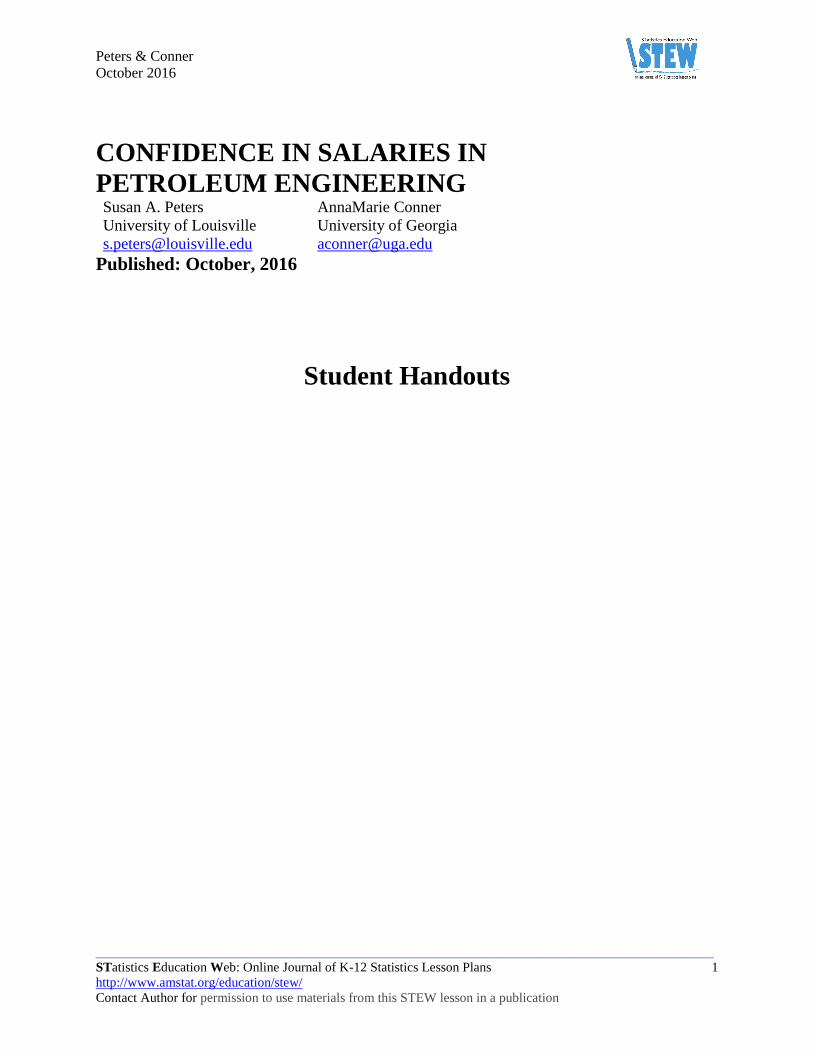
To find a reasonable interval estimate for a population mean, we need to
select many samples and calculate their sample means. (In reality, we
would want to select all possible resamples to know all possible means
that could result from samples of the population, but doing so often is
impractical. Instead, we work with a large number of resamples.) We
simulate the process for the sake of efficiency.
We will use 16 cards from a deck of cards to represent specific salaries in
order to simulate sampling with replacement from our sample of 16
salaries. In particular, we will use the aces and face cards of the four card
suits to represent each of the salaries as shown on the next page. To
begin, remove the aces and face cards from your deck of cards.
1. Simulate the selection of a sample of size 16 using resampling.
a. Shuffle the 16 aces and face cards, and randomly select one of the cards.
b. Record a tally mark for this card in the appropriate box for Sample 1 on the next page.
c. Replace the card.
d. Repeat the selection and recording process (a-c) 15 more times until you have a total of
16 tally marks.
e. Calculate the mean for the 16 salaries selected, and record the value in the table.
2. Compare and contrast this bootstrap sample with the original sample of size 16. Focus on the
distribution of values and on the mean.
3. Repeat the resampling process (#1) three more times, recording your results in the tables on
the next page.
4. Examine the four means that you calculated for your four bootstrap samples by first plotting
the means on a dotplot. Use these means to suggest an interval estimate for the mean starting
salary of the population of petroleum engineering graduates.
5. Would your estimate change if you had calculated additional means? Why or why not?
http://www.numericana.com/answer/cards.htm

Peters & Conner
October 2016
_____________________________________________________________________________________________
STatistics Education Web: Online Journal of K-12 Statistics Lesson Plans 6
http://www.amstat.org/education/stew/
Contact Author for permission to use materials from this STEW lesson in a publication
Resampling Simulation
Card Hearts Clubs Diamonds Spades
Ace King Queen Jack Ace King Queen Jack Ace King Queen Jack Ace King Queen Jack
Salary $93,499 $90,008 $89,719 $89,401 $88,730 $88,238 $87,475 $87,306 $87,002 $85,923 $85,193 $84,682 $83,623 $83,584 $83,063 $79,499
Sample 1
Card Hearts Clubs Diamonds Spades
Ace King Queen Jack Ace King Queen Jack Ace King Queen Jack Ace King Queen Jack
Salary $93,499 $90,008 $89,719 $89,401 $88,730 $88,238 $87,475 $87,306 $87,002 $85,923 $85,193 $84,682 $83,623 $83,584 $83,063 $79,499
Tally
Mean
Sample 2
Card Hearts Clubs Diamonds Spades
Ace King Queen Jack Ace King Queen Jack Ace King Queen Jack Ace King Queen Jack
Salary $93,499 $90,008 $89,719 $89,401 $88,730 $88,238 $87,475 $87,306 $87,002 $85,923 $85,193 $84,682 $83,623 $83,584 $83,063 $79,499
Tally
Mean
Sample 3
Card Hearts Clubs Diamonds Spades
Ace King Queen Jack Ace King Queen Jack Ace King Queen Jack Ace King Queen Jack
Salary $93,499 $90,008 $89,719 $89,401 $88,730 $88,238 $87,475 $87,306 $87,002 $85,923 $85,193 $84,682 $83,623 $83,584 $83,063 $79,499
Tally
Mean
Sample 4
Card Hearts Clubs Diamonds Spades
Ace King Queen Jack Ace King Queen Jack Ace King Queen Jack Ace King Queen Jack
Salary $93,499 $90,008 $89,719 $89,401 $88,730 $88,238 $87,475 $87,306 $87,002 $85,923 $85,193 $84,682 $83,623 $83,584 $83,063 $79,499
Tally
Mean

Peters & Conner
October 2016
_____________________________________________________________________________________________
STatistics Education Web: Online Journal of K-12 Statistics Lesson Plans 7
http://www.amstat.org/education/stew/
Contact Author for permission to use materials from this STEW lesson in a publication
6. Record the value of each mean you calculated on a separate post-it note. Use your post-it
notes to plot your four means on the class display. Examine the class distribution of means,
and record it below.
7. Use the class means to suggest an interval estimate for the mean starting salary of the
population of petroleum engineering graduates.
8. Compare and contrast this interval estimate with your estimate from #4.
9. With which estimate are you more confident that you have accurately captured the
population mean starting salary for petroleum engineering graduates, and why?
10. How many means were recorded on your dotplot in #6?

Peters & Conner
October 2016
_____________________________________________________________________________________________
STatistics Education Web: Online Journal of K-12 Statistics Lesson Plans 8
http://www.amstat.org/education/stew/
Contact Author for permission to use materials from this STEW lesson in a publication
Bootstrapping for Confidence
To find an accurate interval estimate for the population mean, we need hundreds
of bootstrap sample means—realistically, 1000 or more. Even though the cards
can help us to select samples quickly, the card process would be quite tedious and
frustrating to use for finding 1000 sample means. We need many more means than
we reasonably can gather from using simulations with materials such as cards.
Instead, we use computing technology to simulate the
selection of 1000 or more samples and calculate their
means to form a bootstrap distribution of means. A nice collection of applets
for resampling, StatKey, is freely available at http://lock5stat.com/statkey/
1. Go to the StatKey website, and under the heading of “Bootstrap Confidence Intervals,” select
the option of “CI for Single Mean, Median, St. Dev.” To generate an interval estimate for the
population mean, often referred to as a confidence interval for the mean, you will first need
to enter the 16 salaries from the original sample by following these steps. As a reminder, the
salaries are: $93,499, $90,008, $89719, $89401, $88730, $88238, $87475 $87306, $87002,
$85923, $85193, $84682, $83623, $83584, $83063, and $79499.
a. Click on the “Edit Data” tab at the top of the screen.
b. Select and delete the data that appear in the “Edit data” window.
c. On the first line, enter the heading of “Salary.”
d. Enter each of the 16 salaries on a separate line below the heading.
e. Double-check your entries, and then click “OK.”
2. This sample is now displayed in the graph labeled as “Original Sample.” Click on the
“Generate 1 Sample” tab to select a single bootstrap sample. You should see the sample
displayed in the graph labeled as “Bootstrap Sample.” The mean of this sample is plotted on
the “Bootstrap Dotplot of Mean” graph. As we noted, we would like 1000 or more bootstrap
sample means from which to estimate the population mean. Rather than repeat the generation
of a single samples 1000 times, we instead will generate 1000 samples by clicking on the
“Generate 1000 Samples” tab. You will not see all 1000 samples, but you will see all of the
means plotted in the bootstrap distribution. What is the mean of these means?
The value of the bootstrap distribution mean should be close to
or approximately equal to the mean of our original sample. We
use the bootstrap distribution to determine our interval estimate
for the population mean. Interval estimates are associated with
a level of confidence for capturing the value of interest from
the population. A common confidence level is 95%, which we
would associate with the interval of values for the middle 95%
of bootstrap sample means. http://www.awinningpersonality.com/self-improvement/emotional-intelligence/5-daily-exercises-boost-keep-confidence/
http://aozoraaira.blogspot.com/2014/10/international-moment-of-frustration.html
http://lock5stat.com/statkey/

Peters & Conner
October 2016
_____________________________________________________________________________________________
STatistics Education Web: Online Journal of K-12 Statistics Lesson Plans 9
http://www.amstat.org/education/stew/
Contact Author for permission to use materials from this STEW lesson in a publication
3. To find the 95% confidence interval for the mean starting salary for petroleum engineers,
click to select the “two-tail” distribution inside the graph area on the upper left side in
StatKey. The endpoints of the interval are displayed on the bootstrap distribution. Record
your interval. We would interpret the interval as follows: We are 95% confident that the
mean starting salary for all petroleum engineers graduating in 2014 is between <lower
endpoint of interval> and <upper endpoint of interval>. Record the interpretation for the
interval you found.
4. Did your interval capture the mean starting salary of $86,266 reported by NACE?
5. Does your interval cause you to question the NACE estimate of $86,266 for the population
mean? Why or why not?

Peters & Conner
October 2016
_____________________________________________________________________________________________
STatistics Education Web: Online Journal of K-12 Statistics Lesson Plans 10
http://www.amstat.org/education/stew/
Contact Author for permission to use materials from this STEW lesson in a publication
Gaining or Losing Confidence
In general, level of confidence is based on long-term behavior associated with
sampling. Our interval estimate was determined by using data from a sample randomly
selected from the population. 95% confidence means that if we were to repeat the
sampling process and the process used to calculate confidence intervals, in the long run,
we would expect 95% of our intervals to capture the value of the population mean.
Because we have no way of knowing the population mean, we will never know whether
our 95% confidence interval successfully captured the mean; we only can state our
confidence level for capturing the mean.
1. Suppose that you would prefer to have a higher level of confidence such as 99%. How do
you think a 99% confidence interval would differ from a 95% confidence interval?
2. Return to StatKey, and click on the value of 0.95 displayed in a blue square in the window
for the bootstrap distribution. Enter “0.99” for 99% confidence, and click “Ok.” Record the
99% confidence interval. How does the 99% confidence interval differ from the 95%
confidence interval?
3. Suppose that you were interested in a lower level of confidence such as 90%. How would a
90% confidence interval differ from the 95% and 99% confidence intervals? Use StatKey to
determine whether the 90% confidence interval matches your expectation.
4. You should have found that a 99% confidence interval is wider than a 95% confidence
interval found using the same sample. Likewise, a 95% confidence interval is wider than a
90% confidence interval. Describe why this relationship makes sense.
5. A sample size of 16 is relatively small. What effect do you think a larger sample size would
have on the 95% confidence interval if the sample characteristics remained the same?
Peters & Conner
October 2016
_____________________________________________________________________________________________
STatistics Education Web: Online Journal of K-12 Statistics Lesson Plans 11
http://www.amstat.org/education/stew/
Contact Author for permission to use materials from this STEW lesson in a publication
Considering the Effects of Sample Size
Small samples reveal greater variability in shape, center, and variation than
larger samples. As a result, smaller samples also reveal greater variability in
estimates for population characteristics. In general, bootstrap distributions will
center on the value of the original sample under consideration; this is less
likely to be the case when bootstrapping from a small sample. For this reason
(and others), statisticians prefer working with larger samples. You may have
noticed a difference between your sample mean and the center of the bootstrap
distribution when you worked with your sample of size 16.
1. Suppose we had selected a random sample of 64 petroleum engineering majors who
graduated in 2014 who reported the following salaries.
89931, 84424, 88501, 84486, 85420, 82618, 91187, 80356, 84020, 85926, 89339, 79041,
82948, 85134, 83727, 84456, 81966, 91112, 80547, 88365, 88232, 88429, 88798, 85410,
87297, 81404, 83795, 83013, 85473. 86270, 83367, 86989, 81648, 85934, 89716, 95127,
84599, 84260, 83519, 92175, 88451, 88036, 79892, 85785, 83022, 91979, 84542, 86263,
79596, 89283, 81663, 86479, 87399, 92901, 84531, 86860, 84135, 83282, 84599, 75773,
91970, 87136, 90598, 87078
Click on the “Edit Data” tab in StatKey. Enter a heading of “Salary” and then each salary on
separate lines OR open a text file that contains the data, and copy and paste the contents into
the data window. Find and record the 95% confidence interval using the bootstrap
distribution from these data, following the same process used for the sample of size 16.
2. Interpret the 95% confidence interval.
3. Did your interval capture the mean starting salary of $86,266 reported by NACE?
4. Does your interval cause you to question the NACE estimate of $86,266 for the population
mean? Why or why not?
http://qbdworks.com/sample-size-question/

Peters & Conner
October 2016
_____________________________________________________________________________________________
STatistics Education Web: Online Journal of K-12 Statistics Lesson Plans 12
http://www.amstat.org/education/stew/
Contact Author for permission to use materials from this STEW lesson in a publication
5. Compare and contrast the 95% confidence interval from the bootstrap distribution for the
sample of size 16 and from the bootstrap distribution for the sample of size 64.
6. Was the bootstrap distribution for the sample size of 64 approximately centered at the mean
of the sample ($85,785)?
7. Calculate the half-width of the 95% confidence interval (half of the interval width or half of
the difference between the upper and lower endpoints) from the sample of size 16 and the
half-width of the 95% confidence interval from the sample of size 64. How are the two half-
widths related?
Another name for the half-width of a confidence interval is margin of
error. The margin of error gives the maximum expected difference
between the population value of interest and the sample estimate for
that value. You may have heard this terminology reported on the news
in relation to election polls. A report stating that a poll predicts a
candidate’s support at 42% with a 5.7% margin of error means that
42% of the sample supported the candidate, and
the population support is estimated to be
between 36.3% and 47.7% with typically 95%
confidence. There is in inverse square root relationship between the
margin of error and sample size. If you wish to halve the width of your
confidence interval or the margin of error, you will need to quadruple the
size of your sample. http://olecommunity.com/election/election-polls/
http://www.zazzle.com.au/error+cushions

Peters & Conner
October 2016
_____________________________________________________________________________________________
STatistics Education Web: Online Journal of K-12 Statistics Lesson Plans 13
http://www.amstat.org/education/stew/
Contact Author for permission to use materials from this STEW lesson in a publication
8. What sample size would be needed to halve the margin of error for a confidence interval
estimate of the population mean starting salary yet again?
9. A precocious student selected a random sample of 256 starting salaries for 2014 petroleum
engineering graduates. The student then followed the process outlined above to create a
bootstrap distribution and 95% confidence interval and achieved the following results.
What approximate value would you expect for the mean of this student’s sample of size 256?
10. Provide an interpretation of the 95% confidence interval for the population mean.
11. Does the interval cause you to question the NACE estimate of $86,266 for the population
mean? Why or why not?
12. What is the margin of error? How does this margin of error relate to the margins of error you
calculated in #7?
Peters & Conner
October 2016
_____________________________________________________________________________________________
STatistics Education Web: Online Journal of K-12 Statistics Lesson Plans 14
http://www.amstat.org/education/stew/
Contact Author for permission to use materials from this STEW lesson in a publication
Bootstrapping for Confidence in Employment
A skeptical student makes the following observation: “Big deal! So
you convinced me that petroleum engineering graduates have average
starting salaries over $85,000. That salary assumes that they actually
can find jobs! What about all of those graduates who aren’t employed?
What good is the salary if I can’t get a job to earn that salary?”
To gain a sense of the percentage of petroleum engineering graduates
that cannot obtain employment, you select a random sample of 277
petroleum engineering graduates and find that 43 of those graduates are
seeking employment currently.
We will use the bootstrapping method to find a 95% confidence interval for the population
proportion of petroleum engineering graduates who are seeking employment. The beauty of
bootstrapping methods is that we follow the same procedures no matter what population
characteristic we wish to estimate! In this case, that means that we would start with our sample
of size 277; treat this sample as the population; and sample with replacement from this sample.
In our simulation, 43 of the 277 sampling units would represent “seeking employment” whereas
234 would represent “employed.” We would select a unit 277 times with replacement and record
the number of “seeking employment” units selected out of the 277 units. We would repeat this
process 1000 or more times and construct a bootstrap distribution of proportions. [The figure of
43 out of 277 graduates currently seeking employment is the number reported by NACE
(2015c).]
1. As before, we will use StatKey to perform the simulation efficiently.
a. From the main StatKey menu, select “CI for Single Proportion” from the “Bootstrap
Confidence Intervals” options.
b. Click to “Edit Data,” and enter the count of 43 for graduates seeking employment from
the sample of size 277.
c. Generate 1000 samples.
d. Find (and record) the 95% confidence interval for the proportion of petroleum
engineering graduates seeking employment.
2. Interpret this 95% confidence interval for the population proportion.
http://www.theepochtimes.com/n3/603148-what-is-unhealthy-skepticism/

Peters & Conner
October 2016
_____________________________________________________________________________________________
STatistics Education Web: Online Journal of K-12 Statistics Lesson Plans 15
http://www.amstat.org/education/stew/
Contact Author for permission to use materials from this STEW lesson in a publication
3. Does the interval cause you to question whether a majority of graduates are seeking
employment currently? Why or why not?
4. What is the margin of error? What does the margin of error tell you?
5. What steps could you take to decrease the margin of error?
Peters & Conner
October 2016
_____________________________________________________________________________________________
STatistics Education Web: Online Journal of K-12 Statistics Lesson Plans 16
http://www.amstat.org/education/stew/
Contact Author for permission to use materials from this STEW lesson in a publication
Try This on your Own
In reality, even though 43 of the 277 petroleum engineering graduates were
seeking employment, not all of the remaining 234 graduates obtained standard
petroleum engineering jobs. Some pursued continuing education studies, while
others entered into military service. Some were only employed part time. Of the
277 graduates, 68.7% were employed full time as petroleum engineers (NACE,
2015c). http://woman.thenest.com/chemical-engineer-vs-petroleum-engineer-14124.html
1. Find a 95% confidence interval for the proportion of petroleum engineering graduates who
are employed full time. Interpret this interval.
2. How would you explain your findings to the skeptical student who questioned whether
graduates could get jobs in petroleum engineering? As part of your response, be sure to
provide complete interpretations of the processes used to find the confidence interval and
why, the confidence interval, and the margin of error.

Peters & Conner
October 2016
_____________________________________________________________________________________________
STatistics Education Web: Online Journal of K-12 Statistics Lesson Plans 17
http://www.amstat.org/education/stew/
Contact Author for permission to use materials from this STEW lesson in a publication
References for Confidence in Salaries in Petroleum Engineering Activities
Cleophas, T. J., Zwinderman, A. H., Cleophas, T. F., & Cleophas, E. P. (2009). Statistics Applied
to Clinical Trials. Dordrecht, The Netherlands: Springer.
Kemp, J. (2014, July 17). Peak petroleum engineer? Or time to still join the boom? Reuters.
Retrieved from http://www.reuters.com/article/2014/07/17/us-usa-engineering-oilandgas-
employment-idUSKBN0FM28520140717
National Association of Colleges and Employers. (2015a). Spring 2015 Salary Survey Executive
Summary. Bethlehem, PA: Author.
National Association of Colleges and Employers. (2015b). First Destinations for the College
Class of 2014. Bethlehem, PA: Author.
National Association of Colleges and Employers. (2015c). Class of 2014 Bachelor Degree
Results. Bethlehem, PA: Author.
Payscale Human Capital. (2015). Petroleum Engineer Salary (United States). Retrieved from
http://www.payscale.com/research/US/Job=Petroleum_Engineer/Salary