Conducting tests for statistically significant differences ... · PDF fileConducting Tests for . Statistically Significant Differences Using Forest Inventory Data. ... FIA began to

United States Department of Agriculture

Forest Service

Northern Research Station

Research Paper NRS-22

Conducting Tests for Statistically Significant Differences Using Forest Inventory DataJames A. WestfallScott A. PughJohn W. Coulston

Visit our homepage at: http://www.nrs.fs.fed.us/

Published by: For additional copies:

USDA FOREST SERVICE USDA Forest Service11 CAMPUS BLVD., SUITE 200 Publications DistributionNEWTOWN SQUARE, PA 19073-3294 359 Main Road Delaware, OH 43015-8640June 2013 Fax: 740-368-0152

Manuscript received for publication January 2013

AbstractMany forest inventory and monitoring programs are based on a sample of ground plots from which estimates of forest resources are derived. In addition to evaluating metrics such as number of trees or amount of cubic wood volume, it is often desirable to make comparisons between resource attributes. To properly conduct statistical tests for differences, it is imperative that analysts fully understand the underlying sampling design and estimation methods, particularly identifying situations where the estimates being compared do not arise from independent samples. Information from the Forest Inventory and Analysis (FIA) program of the U.S. Forest Service was used to demonstrate circumstances where samples were not independent, and correct calculation of the standard error (and associated confidence intervals) required accounting for covariance. Failure to include the covariance when making comparisons between attributes resulted in standard errors that were too small. Conversely, comparisons of the same attribute at two points in time suffered from exaggerated standard errors when the covariance was excluded. The results indicated the effect of the covariance depends on the attribute of interest as well as the structure of the population being sampled.

AuthorsJAMES A. WESTFALL is a research forester with the U.S. Forest Service, Northern Research Station, 11 Campus Boulevard, Newtown Square, PA 19073. Phone: 610-557-4043, email: [email protected].

SCOTT A. PUgH is a forester with the U.S. Forest Service, Northern Research Station, 410 MacInnes Drive, Houghton, MI 49931.

JOHN W. COULSTON is a supervisory research forester with the U.S. Forest Service, Southern Research Station, 4700 Old Kingston Pike, Knoxville, TN 37919.

�

INTRoDUCTIoNMany nations have implemented a national forest inventory (NFI) to assess and monitor forest resources (Gillis et al. 2005, Tomppo 2006). Also, in response to initiatives such as UN REDD�, many other countries are currently developing NFI programs (Maniatis and Mollicone 20�0). A key output of nearly all NFI efforts is sample-based estimates for attributes of interest (e.g., forest land area or net cubic volume). Apart from providing a current evaluation of relevant forest characteristics, other primary uses of these estimates include making comparisons between current values and evaluating change over time. For example, the differences in tree density between two species may be of interest, or it may be useful to assess changes in forest land area between successive inventory cycles. Such inquiries provide valuable information that is often used to guide management and policy decisions that can have wide-ranging effects on forest resources. Due to the broad and complex nature of many NFIs (Tomppo et al. 20�0), the number of comparisons that can be made is nearly limitless.

Because of an increased emphasis on estimates of change, many NFI programs have fixed plot locations that are remeasured over time (Brassel and Lischke 200�, Reams et al. 2005). Furthermore, sometimes a country’s area is divided into smaller subpopulations to facilitate estimation at finer spatial scales. These factors can substantially increase the statistical complexity of making comparisons because certain circumstances may result in estimates arising from samples that are not independent. Specifically, the lack of independence requires that a covariance term be accounted for when computing the standard error of the difference between two attributes (Husch et al. �982). However, in many cases, the only knowledge at hand for each attribute is the estimate and associated

� The United Nations program for Reducing Emissions from Deforestation and Forest Degradation (REDD) promotes retention of forest carbon in developing countries.

standard error while the covariance is unavailable. Analysts should be aware of limitations regarding how these statistics can be extended into hypothesis testing for statistically significant differences. In order to ensure proper calculations, the analyst must thoroughly understand both the sample design and associated estimation procedures inherent to the NFI data being examined. This paper utilized the NFI conducted in the United States to illustrate some pitfalls to be avoided and appropriate techniques to employ when making spatial and temporal comparisons between estimates.

BACkgRoUNDThe Forest Inventory and Analysis (FIA) program of the U.S. Forest Service is charged with providing data and analyses to assess and monitor the nation’s forest resources. Traditionally, FIA conducted periodic inventories in each state every �0-�5 years. In �999, FIA began to implement an annual inventory system as mandated by the �998 Farm Bill (Public Law �05-�85). This change affected almost all facets of the program. Particularly, the annual system required a new sample design, new estimation procedures (Bechtold and Patterson 2005), as well as the need to perform data distribution and analyses tasks yearly for each state.

FIA puts forth considerable effort to ensure data are available to the public in a timely manner. In order to facilitate the use of these data, FIA also provides analytical software that generates estimates and associated sampling errors. These tools have a wide range of analytical flexibility to generate tables of estimates for current conditions as well as growth, removals, and mortality (GRM) over time and are widely used to perform the complex data queries and statistical calculations needed to correctly analyze the data. The estimates and associated sampling errors generated by FIA analytical tools are reliable information that can be used to support scientific investigations and provide a basis for making management and policy decisions.

2

INveNToRy DeSIgNFIA implements a three-phase forest inventory and monitoring effort (Bechtold and Patterson 2005). Phase one (P�) is the development of a poststratification scheme using remotely-sensed data in order to reduce variance in the estimates. Under the current FIA sampling design where plot locations are fixed over time, stratification occurs after the plot locations are selected, thus the term poststratification. Geospatial data, typically derived from National Land Cover Database products (Fry et al. 20��, Homer et al. 2007), are used to create nonoverlapping strata. Each plot is assigned to a stratum via spatial overlay, and the strata weights are the proportion of the population occupied by each strata. The second phase (P2) of data collection entails measuring sample plots on the ground for the usual suite of forest mensuration variables such as tree species, diameter at breast height (d.b.h.), height, site index, forest type, and stand age. For each sample plot, trees with a d.b.h. of 5.0 inches or larger are measured on four subplots having a 24 ft radius; saplings with a d.b.h. of �.0-4.9 inches are measured on four microplots having a 6.8 ft radius (Bechtold and Scott 2005). Phase three (P3) data

collection occurs on a �/�6th subset of the P2 plots and includes measuring additional forest health indicators (e.g., down woody material and crown condition information). A key point here is that differing conditions on a plot are mapped. For the purposes of this paper, it is sufficient to understand that a plot can have more than one forest type, and the area and the trees within those types can be identified. It is also important to understand that nonforest portions of plots, including plots that are entirely nonforest, are part of the sample. In the case of entirely nonforest plots, the area of forest conditions is zero and plot-level summaries of other traditional plot attributes (e.g., cubic volume of wood) are also zero.

Under the annual inventory system, a percentage of the sample plots (generally 20 percent in the eastern United States and �0 percent in the western United States) are measured each year. The set of plots measured within a single year is referred to as a panel (Fig. �). Once all plots have been measured, they are placed into groups representing the most recent measurement of each plot. In the east, for example, it takes 5 years to measure all plots, so years �-5

Figure 1.—Schematic of a five panel design implemented over 5-year inventory cycles. Each letter (a, b, c, d, and e) represents a separate panel.

3

are grouped initially, then years 2-6, 3-7, and so on (Fig. �). This creates a moving timeline of data for analytical purposes. Also, the grouping of years �-5 is considered the first inventory cycle, years 6-�0 is the second cycle, and so on (Fig. �). To facilitate estimation, independent subpopulations within states are created and are usually defined by administrative boundaries such as counties or groups of counties. In FIA, these subpopulations are referred to as estimation units, and it is at this level that estimation is carried out, i.e., the stratification is performed and applied within each estimation unit and all plots within the unit contribute to making estimates. One method FIA employs to define strata uses canopy cover classes (e.g., 0-5 percent up to 8�-�00 percent cover). Estimates for attributes such as volume or area can be further refined by using domain variables such as tree species, diameter class, or forest type (Scott et al. 2005). Because estimation units define independent subpopulations, estimates across these subpopulations are easily combined for estimates of larger geographic scope (e.g., a state).

ISSUeSIssue 1: Comparing estimates over time within a single estimation unitStandard FIA analytical tools, such as EVALIDator (Miles 20�2), follow the estimation methods described above. Because of the repeated measurement of panels, samples are often not independent. When testing for differences in estimates over time for a single estimation unit, any instance where the same letters (Fig. �) are used to construct the estimates requires covariance to be accounted for. Focusing on Figure �, consider the comparison of one estimate constructed from the set of observations in solid grey (in EVALIDator this is referred to as the year 5 estimate) to another estimate constructed by the observations outlined by the black box (referred to as the year 7 estimate in EVALIDator). The year 5 estimate uses the following set of observations: ayear�, byear2, cyear3, dyear4,

and eyear5. The year 7 estimate uses the following set of observations: cyear3, dyear4, eyear5, ayear6, byear7. Note that the same set of plots (panels a-e) is used for both the year 5 and the year 7 estimates with observations in panels c, d, and e being the same and observations in the remaining panels (a and b) being from the same plots at different points in time. When comparing the year 5 estimate (constructed from observations in ayear�, byear2, cyear3, dyear4, and eyear5) to the year �0 estimate (constructed from observations in ayear6, byear7, cyear8, dyear9, and eyear�0), the observations in ayear6 are remeasurements of the same plots that were observed in ayear� and likewise for b, c, d, and e. Although the observed plot data may differ between the two samples, these samples are entirely dependent because the same set of plots makes up each sample. In both cases described above, the researcher should account for the covariance when computing the standard error of the difference between estimates. In cases where samples are entirely dependent, the standard formula for calculating covariance can be used (Schreuder et al. 2004). For more complex situations where only a portion of the plots are common to both samples (partially-dependent), an adjustment factor should be employed (Kish �995, Zheng 2004). We note that comparisons between estimates constructed using observations with different letters (e.g., ayear� compared to dyear4) can be made assuming independent samples; however, these types of comparisons are typically not of interest to most analysts. Issue 2: Comparing current estimates within or between estimation unitsUnderstanding and reporting how resources differ spatially within or between estimation units is fundamental to forest analytics. We address two cases that arise when comparing estimates spatially using FIA’s online tools: �) comparing estimates of totals or ratios within estimation units, and 2) comparing estimates of totals or ratios from separate estimation units.

4

First, we compare population totals and ratios within a single estimation unit. Estimation unit � (EU�) in Figure 2 is an extension of Figure � over space. Our objective is to compare the estimate of hardwood forest type area to the estimate of conifer forest type area within EU�. In Figure 2, the green letters denote conifer forest type samples, and the rust letters denote hardwood forest type samples. To construct an estimate of the hardwood forest type area, all the plots are used including nonforest plots (denoted in blue). The estimate of the hardwood forest type area for EU� is obtained by dividing the observed hardwood forest plot area by the total observed plot area (forest and nonforest) within each stratum, calculating a weighted average across strata, and multiplying by the area of EU�. Note that conditions that are not hardwood forest types are recorded as zeros, and these zeros are included in both the calculation of the estimate and its standard error. The estimate for the area of softwood forest type is constructed likewise. Hence, the set of plots are the same for both the hardwood and softwood types described above, and the covariance should be accounted for. This also holds true for ratio estimates such as volume per acre. When comparing the volume per acre of forest in hardwood type to the volume per acre of forest in conifer type, both ratio estimates require using all the plots in EU�, so when making comparisons between them, the covariance should be accounted for (Cochran �977).

The same concepts described in the preceding paragraph are relevant when comparing estimates for discrete subareas within an estimation unit to estimates obtained for the entire unit. Consider EU� in Figure 2 where the gray shaded area represents a national forest (EU�NF) which is a discrete subarea but not an estimation unit or a stratum. Suppose our objective is to compare the volume per acre of forest within EU�NF to the volume per acre of forest in EU�. This situation is also a domain analysis, and in this case, the sample used to estimate volume per acre of forest within EU�NF includes the same plots used to estimate the volume per acre of forest within EU�, so covariance should be accounted for. As a general rule, when

Figure 2.—Schematic of a five panel design for two estimation units (EU1 and EU2). Panels 1 through 5 are represented by letters a through e. The green letters represent conifer forest types, the rust letters represent hardwood forest types, and the blue letters represent nonforest. The area shaded gray represents a single national forest (EU1NF) within estimation unit EU1.

5

comparing domains within an estimation unit, analysts must account for covariance. If EU�NF is identified as a separate stratum during the poststratification process, analysts may be able to treat EU�NF as an independent sample from the area identified by the portion of EU� that does not contain EU�NF (EU� – EU�NF). In fact, one can generally consider samples from different strata within an estimation unit as independent; however, these types of analyses are difficult to conduct using the standard FIA analytical tools because stratum-level estimates are not included in the output information.

Next, we compare estimates of population totals (e.g., hardwood forest type area) or ratios (e.g., hardwood volume per acre of forest) between two estimation units. For example, estimation units EU� and EU2 in Figure 2 have no plots in common to both samples and are defined as independent subpopulations. Therefore, the samples from EU� and EU2 are independent, covariance cannot be calculated because there are no common plots by which to do so, and covariance is zero by definition.

eRRoR PRoPAgATIoNThe issues previously raised are intended to help users of FIA data that rely on tools such as EVALIDator to decide if samples are dependent or independent. The intent now is to elucidate appropriate error propagation techniques under each scenario and to provide an example of how analytical results can be misleading by improperly propagating errors. The appropriate formula for the standard error of the difference (sx–y ) between random variables x and y is:

[�]

where

s2x = sample-based variance of the estimate for x,

s2y = sample-based variance of the estimate for y, and

sxy = sample-based covariance between x and y.

There are two important points regarding the formula above: �) when the estimates of x and y arise from independent samples, the covariance is zero by definition, and thus the third term disappears, and 2) when the covariance is positive, the effect is to make the standard error smaller (and vice versa). With this in mind, a problematic situation arises when testing for differences using FIA data (and by extension, possibly other forest inventory data). Suppose an analyst wants to determine whether the area of hardwood forest types is different than the area of conifer forest types. On any given plot, there is a fixed amount of area such that if the area of hardwood forest type increases, then the area of conifer forest type decreases. In fact, many plots will be entirely in only one of these two types. Because of this explicit relationship, the covariance will be negative. When the negative covariance is not accounted for (i.e., the estimates are treated as independent), the resultant sampling error will be too small.

As a practical matter, the information provided by EVALIDator essentially only allows analysts to construct confidence intervals for each estimate. This often leads to testing whether there are differences between the estimates by comparing the confidence intervals (CI) and determining if there is any overlap. If there is no overlap, it is concluded that the two estimates are statistically different. There are two reasons why this method is not appropriate: �) the overlapping CI method assumes the estimates are obtained from independent samples, which is not the case in many instances, and 2) even for independent samples, the overlapping CI method may indicate there is no difference when proper computation of the standard error of the difference would result in the conclusion of a significant difference (Schenker and Gentleman 200�). Thus, analysts should be particularly wary of drawing conclusions when confidence intervals from independent samples overlap because the overlapping confidence interval approach suggests that the standard errors are additive (i.e., sx–y = sx + sy ) rather than the

6

variances being additive as denoted in equation [�]. Since , the width of the confidence interval of the difference is too wide. As such, it is recommended that analysts do not employ the overlapping CI method.

In most cases, online tools present percent sampling error rather than the standard error of the estimate or the variance of the estimate. However, the formulas described here rely on the variance of the estimate. It is straightforward to calculate the standard error of the estimate (sy ) from the percent sampling error (SE%) and the estimate (y). SE% =�00(sy /y) and therefore sy = SE% × (y/�00). This simple calculation will facilitate appropriate error propagation.

CASe exAmPleSAn empirical evaluation of the issues described above was performed for each of �3 states in the Northeastern United States. Initial analyses conducted included �) a comparison of the area proportions between hardwood and conifer forest types, and 2) a comparison of the area proportions between maple/beech/birch (MBB) and conifer forest types. Failing to properly account for the covariance when comparing the proportions of hardwood and conifer forest types produced standard errors that were 20-30 percent too small (Table �). If 95 percent confidence intervals were constructed using the incorrect standard errors, the resultant intervals would represent confidence levels between 83-88 percent. The results of the second analysis (Table 2) indicated the underestimate of the standard error ranged from approximately 3-23 percent. Again, 95 percent confidence intervals would also be too small (actually 87-94 percent). These results showed that the effect of the covariance on the standard error �) depended on the specific comparison being made, and 2) depended on the structure of the population being sampled. Therefore, it is not possible to make any broad statements about the magnitude of influence the covariance may have on the standard error.

Table 1.—Standard errors for assumed independent (SeI) and dependent (SeD) samples, the percent difference, and the effective 95 percent confidence interval coverage for SeI when estimating the difference in area proportions between hardwood and conifer forest types for 13 Northeastern states.

State SEI SED Diff. (%) CL95eff (%)

CT 0.0290 0.0379 23.38 86.6DE 0.0202 0.0286 29.29 83.4ME 0.0107 0.0151 29.29 83.4MD 0.0173 0.0227 23.69 86.5MA 0.0245 0.0323 24.24 86.2NH 0.0203 0.0282 28.06 84.1NJ 0.0206 0.0272 24.11 86.2NY 0.0075 0.0105 29.28 83.4OH 0.0068 0.0087 21.36 87.6PA 0.0071 0.0100 29.29 83.4RI 0.0416 0.0541 23.16 86.7VT 0.0216 0.0285 24.14 86.2WV 0.0121 0.0161 24.39 86.1

Table 2.—Standard errors for assumed independent (SeI) and dependent (SeD) samples, the percent difference, and the effective 95 percent confidence interval coverage for SeI when estimating the difference in area proportions between maple/beech/birch (mBB) and conifer forest types for 13 Northeastern states.



7

When attributes of interest are on a per unit area basis, the phenomenon of negative covariance due to plot area constraints largely disappears. For example, if a plot is partly hardwood forest type and partly conifer forest type, the basal area per acre for one forest type is not constrained by the other. In this case, anticipating the sign of the covariance is not as intuitive. It is now useful to recall that all plots in the estimation unit are used for every estimate. Furthermore, using the hardwood and conifer forest type example, a majority of plots will have one forest type but not the other. Thus, the structure of most of the data will be a zero for one forest type and a positive number for the other, a situation conducive to negative covariance. To empirically illustrate this concept, the same two analyses described above were conducted using basal area per acre of live trees (BALIVE) (see Woudenberg et al. 20�0) as the attribute of interest. Specifically, it was desired to test for significant differences in mean basal area per acre between �) hardwood and conifer forest types, and 2) MBB and conifer forest types. Although the analysis was based on a different attribute, the results were similar to the previous outcome using forest type area. Table 3 shows that standard errors were again consistently underestimated when covariance was not accounted for. However, unlike the area comparisons between hardwood and softwood forest types (Table �), the underestimation ranged from 3-23 percent when comparing basal area per acre (Table 3). Calculation of 95 percent confidence intervals produced intervals that were actually in the 87-94 percent range. The comparison of mean basal area per acre between MBB and conifer types (Table 4) provided further confirmation of consistently negative covariance, with effects on standard errors depending on the comparison being made and the underlying population structure.

It is often of considerable importance to evaluate the change in an attribute over time. For these types of analyses, the covariance would likely be positive,

Table 3.—Standard errors for assumed independent (SeI) and dependent (SeD) samples, the percent difference, and the effective 95 percent confidence interval coverage for SeI when estimating the difference in mean basal area per acre between hardwood and conifer forest types for 13 Northeastern states.



Table 4.—Standard errors for assumed independent (SeI) and dependent (SeD) samples, the percent difference, and the effective 95 percent confidence interval coverage for SeI when estimating the difference in mean basal area per acre between maple/beech/birch (mBB) and conifer forest types for 13 Northeastern states.



8

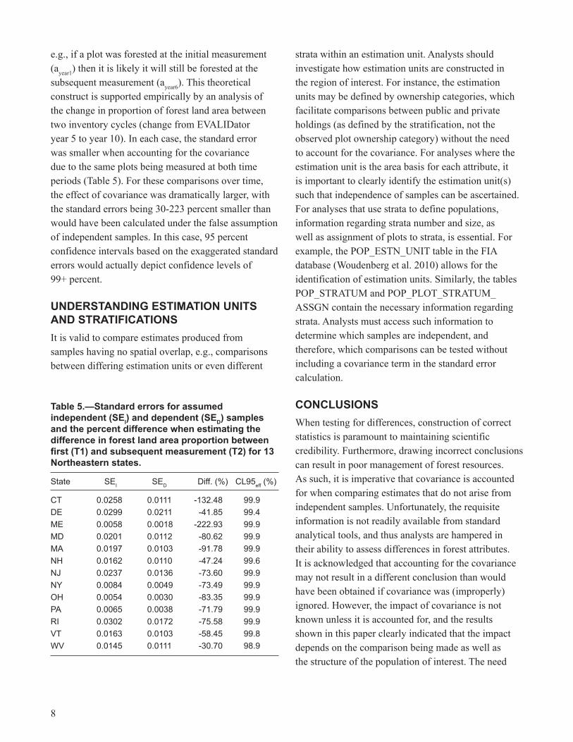
e.g., if a plot was forested at the initial measurement (ayear�) then it is likely it will still be forested at the subsequent measurement (ayear6). This theoretical construct is supported empirically by an analysis of the change in proportion of forest land area between two inventory cycles (change from EVALIDator year 5 to year �0). In each case, the standard error was smaller when accounting for the covariance due to the same plots being measured at both time periods (Table 5). For these comparisons over time, the effect of covariance was dramatically larger, with the standard errors being 30-223 percent smaller than would have been calculated under the false assumption of independent samples. In this case, 95 percent confidence intervals based on the exaggerated standard errors would actually depict confidence levels of 99+ percent.

UNDeRSTANDINg eSTImATIoN UNITS AND STRATIFICATIoNSIt is valid to compare estimates produced from samples having no spatial overlap, e.g., comparisons between differing estimation units or even different

Table 5.—Standard errors for assumed independent (SeI) and dependent (SeD) samples and the percent difference when estimating the difference in forest land area proportion between first (T1) and subsequent measurement (T2) for 13 Northeastern states.


CT 0.0258 0.0111 -132.48 99.9DE 0.0299 0.0211 -41.85 99.4ME 0.0058 0.0018 -222.93 99.9MD 0.0201 0.0112 -80.62 99.9MA 0.0197 0.0103 -91.78 99.9NH 0.0162 0.0110 -47.24 99.6NJ 0.0237 0.0136 -73.60 99.9NY 0.0084 0.0049 -73.49 99.9OH 0.0054 0.0030 -83.35 99.9PA 0.0065 0.0038 -71.79 99.9RI 0.0302 0.0172 -75.58 99.9VT 0.0163 0.0103 -58.45 99.8WV 0.0145 0.0111 -30.70 98.9

strata within an estimation unit. Analysts should investigate how estimation units are constructed in the region of interest. For instance, the estimation units may be defined by ownership categories, which facilitate comparisons between public and private holdings (as defined by the stratification, not the observed plot ownership category) without the need to account for the covariance. For analyses where the estimation unit is the area basis for each attribute, it is important to clearly identify the estimation unit(s) such that independence of samples can be ascertained. For analyses that use strata to define populations, information regarding strata number and size, as well as assignment of plots to strata, is essential. For example, the POP_ESTN_UNIT table in the FIA database (Woudenberg et al. 20�0) allows for the identification of estimation units. Similarly, the tables POP_STRATUM and POP_PLOT_STRATUM_ASSGN contain the necessary information regarding strata. Analysts must access such information to determine which samples are independent, and therefore, which comparisons can be tested without including a covariance term in the standard error calculation.

CoNClUSIoNSWhen testing for differences, construction of correct statistics is paramount to maintaining scientific credibility. Furthermore, drawing incorrect conclusions can result in poor management of forest resources. As such, it is imperative that covariance is accounted for when comparing estimates that do not arise from independent samples. Unfortunately, the requisite information is not readily available from standard analytical tools, and thus analysts are hampered in their ability to assess differences in forest attributes. It is acknowledged that accounting for the covariance may not result in a different conclusion than would have been obtained if covariance was (improperly) ignored. However, the impact of covariance is not known unless it is accounted for, and the results shown in this paper clearly indicated that the impact depends on the comparison being made as well as the structure of the population of interest. The need

9

to account for covariance when the samples are not independent is well established in statistical theory; however, a failure to understand FIA sampling and estimation may result in this need going unrecognized. Even with the understanding that covariance needs to be accounted for in many comparative analyses, the range of skills and knowledge needed to do so makes it a challenging endeavor to undertake. To facilitate proper statistical calculations needed for comparative tests of hypotheses, further development of tools such as EVALIDator is needed. While the statistical formulas are known, the actual implementation into a functional, user-friendly application may be difficult due to the wide range of comparisons that analysts can evaluate.

lITeRATURe CITeDBechtold, W.A.; Patterson, P.L., eds. 2005. The

enhanced Forest Inventory and Analysis program-national sampling design and estimation procedures. Gen. Tech. Rep. SRS-80. Asheville, NC: U.S. Department of Agriculture, Forest Service, Southeastern Research Station. 85 p.

Bechtold, W.A.; Scott, C.T. 2005. The Forest Inventory and Analysis plot design. In: Bechtold, W.A.; Patterson, P.L., eds. The enhanced Forest Inventory and Analysis program - national sampling design and estimation procedures. Gen. Tech. Rep. SRS-80. Asheville, NC: U.S. Department of Agriculture, Forest Service, Southeastern Research Station: 37-52.

Brassel, P.; Lischke, H., eds. 200�. Swiss national forest inventory: methods and models of the second assessment. Birmensdorf, Switzerland: Swiss Federal Research Institute WSL. 336 p.

Cochran, W.G. �977. Sampling techniques. 3rd ed. New York, NY: John Wiley & Sons, Inc. 428 p.

Fry, J.A.; Xian, G.; Suming, J.; Dewitz, J.A.; Homer, C.G.; Yang, L.; Barnes, C.A.; Herold, N.D.; Wickham, J.D. 20��. Completion of the 2006 national land cover database for the conterminous United States. Photogrammetric Engineering and Remote Sensing. 77(9): 858-864.

Gillis, M.D.; Omule, A.Y.; Brierley, T. 2005. Monitoring Canada’s forests: the national forest inventory. The Forestry Chronicle. 8�: 2�4-22�.

Homer, C.; Dewitz, J.; Fry, J.; Coan, M.; Hossain, N.; Larson, C.; Herold, N.; McKerrow, A.; VanDriel, J.N.; Wickham, J. 2007. Completion of the 2001 National Land Cover Database for the conterminous United States. Photogrammetric Engineering & Remote Sensing. 73(4): 337-34�.

Husch, B.; Miller, C.I.; Beers, T.W. �982. Forest mensuration. New York, NY: John Wiley & Sons, Inc. 402 p.

Kish, L. �995. Survey sampling. Classics ed. New York, NY: John Wiley & Sons, Inc. 643 p.

Maniatis, D.; Mollicone, D. 20�0. Options for sampling and stratification for national forest inventories to implement REDD+ under the UNFCCC. Carbon Balance and Management. 5: 9. DOI: �0.��86/�750-0680-5-9.

Miles, P.D. 20�2. Forest Inventory EVALIDator web-application version 1.5.1.2a. St. Paul, MN: U.S. Department of Agriculture, Forest Service, Northern Research Station. Available at: http://apps.fs.fed.us/Evalidator/tmattribute.jsp. [Date accessed unknown].

Reams, G.A.; Smith, W.D.; Hansen, M.H.; Bechtold, W.A.; Roesch, F.A.; Moisen, G.G. 2005. The Forest Inventory and Analysis sampling frame. In: Bechtold, W.A.; Patterson, P.L., eds. The enhanced Forest Inventory and Analysis program-national sampling design and estimation procedures. Gen. Tech. Rep. SRS-80. Asheville, NC: U.S. Department of Agriculture, Forest Service, Southeastern Research Station: ��-26.

�0

Schenker, N.; Gentleman, J.F. 200�. On judging the significance of differences by examining the overlap between confidence intervals. The American Statistician. 55: �82-�86.

Schreuder, H.T.; Ernst, R.; Ramirez-Maldonado, H. 2004. Statistical techniques for sampling and monitoring natural resources. Gen. Tech. Rep. RMRS-�26. Fort Collins, CO: U.S. Department of Agriculture, Forest Service, Rocky Mountain Research Station. �� p.

Scott, C.T.; Bechtold, W.A.; Reams, G.A.; Smith, W.D.; Westfall, J.A.; Hansen, M.H.; Moisen, G.G. 2005. Sample-based estimators used by the Forest Inventory and Analysis national information management system. In: Bechtold, W.A.; Patterson, P.L., eds. The enhanced Forest Inventory and Analysis program-national sampling design and estimation procedures. Gen. Tech. Rep. SRS-80. Asheville, NC: U.S. Department of Agriculture, Forest Service, Southeastern Research Station: 43-67.

Tomppo, E. 2006. The Finnish national forest inventory. In: Kangas, A.; Maltamo, M., eds. Forest inventory: methodology and applications. Dordrecht, Netherlands: Springer: �79-�94. Vol. �0.

Tomppo, E.; Gschwantner, T.; Lawrence, M.; McRoberts, R.E., eds. 20�0. National Forest inventories-pathways for common reporting. New York, NY: Springer. 6�2 p.

Woudenberg, S.W.; Conkling, B.L.; O’Connell, B.M.; LaPoint, E.B.; Turner, J.A.; Waddell, K.L. 20�0. The Forest Inventory and Analysis database: database description and users manual version 4.0 for Phase 2. Gen. Tech. Rep. RMRS-GTR-245. Fort Collins, CO: U.S. Department of Agriculture, Forest Service, Rocky Mountain Research Station. 336 p.

Zheng, B. 2004. Poverty comparisons with dependent samples. Journal of Applied Econometrics. �9: 4�9-428.

The U.S. Department of Agriculture (USDA) prohibits discrimination in all its programs and activities on the basis of race, color, national origin, age, disability, and where applicable, sex, marital status, familial status, parental status, religion, sexual orientation, genetic information, political beliefs, reprisal, or because all or part of an individual’s income is derived from any public assistance program. (Not all prohibited bases apply to all programs.) Persons with disabilities who require alternate means for communication of program information (Braille, large print, audiotape, etc.) should contact USDA’s TARgET Center at (202) 720-2600 (voice and TDD). To file a complaint of discrimination, write to USDA, Director, Office of Civil Rights, 1400 Independence Avenue, S.W., Washington, DC 20250-9410, or call (800) 795-3272 (voice) or (202) 720-6382 (TDD). USDA is an equal opportunity provider and employer.

Printed on recycled paper

Westfall, James A.; Pugh, Scott A.; Coulston, John W. 2013. Conducting tests for statistically significant differences using forest inventory data. Res. Pap. NRS-22. Newtown Square, PA: U.S. Department of Agriculture, Forest Service, Northern Research Station. 10 p.

Many forest inventory and monitoring programs are based on a sample of ground plots from which estimates of forest resources are derived. In addition to evaluating metrics such as number of trees or amount of cubic wood volume, it is often desirable to make comparisons between resource attributes. To properly conduct statistical tests for differences, it is imperative that analysts fully understand the underlying sampling design and estimation methods, particularly identifying situations where the estimates being compared do not arise from independent samples. Information from the Forest Inventory and Analysis (FIA) program of the U.S. Forest Service was used to demonstrate circumstances where samples were not independent, and correct calculation of the standard error (and associated confidence intervals) required accounting for covariance. Failure to include the covariance when making comparisons between attributes resulted in standard errors that were too small. Conversely, comparisons of the same attribute at two points in time suffered from exaggerated standard errors when the covariance was excluded. The results indicated the effect of the covariance depends on the attribute of interest as well as the structure of the population being sampled.

KEY WORDS: covariance, confidence interval, sampling design, hypothesis test, change estimation

Northern Research Station

www.nrs.fs.fed.us

Documents

Conducting tests for statistically significant differences ... · PDF fileConducting Tests for . Statistically Significant Differences Using Forest Inventory Data. ... FIA began to