Condition monitoring opportunities using vehicle … University Institutional Repository Condition monitoring opportunities using vehicle-based sensors This item was submitted to Loughborough

Loughborough UniversityInstitutional Repository

Condition monitoringopportunities usingvehicle-based sensors

This item was submitted to Loughborough University's Institutional Repositoryby the/an author.

Citation: WARD, C.P. ... et al, 2010. Condition monitoring opportunitiesusing vehicle-based sensors. Proceedings of the Institution of Mechanical Engi-neers, Part F: Journal of Rail and Rapid Transit, 225 (2), pp. 202-218.

Metadata Record: https://dspace.lboro.ac.uk/2134/6643

Version: Published

Publisher: c© Professional Engineering Publishing

Please cite the published version.

https://dspace.lboro.ac.uk/2134/6643

This item was submitted to Loughborough’s Institutional Repository (https://dspace.lboro.ac.uk/) by the author and is made available under the

following Creative Commons Licence conditions.

For the full text of this licence, please go to: http://creativecommons.org/licenses/by-nc-nd/2.5/

SPECIAL ISSUE PAPER 1

Condition monitoring opportunitiesusing vehicle-based sensorsC P Ward1, P F Weston2, E J C Stewart2, H Li3, R M Goodall1∗, C Roberts2, T X Mei4, G Charles5, and R Dixon1

1Control Systems Group, Electronic and Electrical Engineering, Loughborough University, Loughborough, UK2Birmingham Centre for Rail Research and Education, The University of Birmingham, Edgbaston, Birmingham, UK3Department of Engineering and Technology, Manchester Metropolitan University, Manchester, UK4School of Computing, Science and Engineering, The University of Salford, Salford, UK5School of Engineering, The University of Nottingham, University Park, Nottingham, UK

The manuscript was received on 16 March 2010 and was accepted after revision for publication on 21 July 2010.

DOI: 10.1243/09544097JRRT406

Abstract: Recent increases in railway patronage worldwide have created pressure on rolling stockand railway infrastructure through the demand to improve the capacity and punctuality of thewhole system, and this demand must also be balanced with reducing life-cycle costs. Conditionmonitoring is seen as a significant contributor in achieving this. The emphasis of this article is onthe use of sensors mounted on rolling stock to monitor the condition of infrastructure and therolling stock itself. This is set in the context of modern rolling stock being fitted with high-capacitycommunication buses and multiple sensors, resulting in the potential for advanced processing ofcollected data. This article brings together linked research that uses a similar set of rolling stocksensors, and discusses: general usage and benefits, a track defect detection method, running gearcondition monitoring, and absolute train speed detection.

Keywords: condition monitoring, real time, vehicle-based sensors, track defects, parameterestimation, low adhesion, wheel–rail profile, vehicle speed, inertial sensors

1 INTRODUCTION

The last two decades have seen widespread increasesin railway patronage worldwide, meaning there issignificant pressure to improve the capacity and punc-tuality of rail services, while reducing life-cycle costs.Condition monitoring systems are seen as a significantcontributor in achieving such improvements.

Broadly speaking, four different types of monitor-ing systems exist: infrastructure-based infrastructuremonitoring, rolling-stock-based infrastructure mon-itoring, rolling-stock-based rolling stock monitoring,and infrastructure-based rolling stock monitoring [1].To date, the use of such approaches for fault detectionand diagnosis purposes has been relatively straight-forward. Dedicated measurement trains are normal inmany railway administrations for assessing the con-dition of the track [2], and there are some examples

∗Corresponding author: Department of Electric and Electronic,

University of Loughborough, Loughborough LE11 3TU, UK.

email: [email protected]

where simplified versions of these measuring systemshave been fitted to service vehicles. For rolling stockmonitoring, some existing fleets have enhanced theiron-board data logging capabilities with global posi-tioning system (GPS) and communications equipment Q1in order to analyse in real-time data from in-servicetrain sets (for example, see references [3] to [5]).

This article is concerned with monitoring based onmeasurements made by sensors fitted to vehicles (i.e.the second and third types described in the previousparagraph, in particular focused upon in-service vehi-cles). Electronic and software systems now form anessential element of railway vehicle technology; sinceit is common for such systems to be connected to acentral control processor through a train communi-cation bus, there is significant potential for advancedprocessing techniques that can extract more sophisti-cated system/sub-system knowledge, either from thesensor data currently available or from additionalsensors connected to the communications bus. Mod-ern wireless communication systems also provide theopportunity for transferring either the raw sensor dataor information derived from such data to track-based

JRRT406 Proc. IMechE Vol. 224 Part F: J. Rail and Rapid Transit

Unco

rrecte

d Pr

oof

2 C P Ward, P F Weston, E J C Stewart, H Li, R M Goodall, C Roberts, T X Mei, G Charles, and R Dixon

information systems that can provide further analysis.However, the emphasis here is upon the potential foradvanced vehicle-based processing.

The purpose of the article is to describe linkedresearch activities all using a relatively common setof vehicle-based sensors combined with advancedprocessing concepts, which are aimed towards dif-ferent technical objectives. Section 2 summarizes theopportunities from a sensing technology viewpointto provide an overview, and then sections 3 to 5describe three specific processing options – identifica-tion of track defects, monitoring of running gear con-dition, and determination of absolute train speed. Theconcluding section summarizes where these develop-ments can contribute at a systems level and identi-fies the longer-term trends arising from the use ofadvanced processing concepts such as these.

2 BOGIE-MOUNTED SENSOR OPTIONS FORMONITORING IN GENERAL – TYPE, LOCATION,NUMBER, AND REQUIREMENTS

Sensors mounted on in-service vehicles can be usedto identify certain track defects, monitor the run-ning gear condition, and determine the absolute trainspeed, all during normal revenue service.

In the case of identifying track defects, the alter-native approach is to use specialist track inspectiontrains. However, due to capacity constraints and theavailability and cost of the inspection train itself, it isdifficult to monitor the whole rail network in a timelyand cost-effective manner.

Table 1 shows an appropriate sensor set for useon in-service vehicles, and this is also illustrated bythe diagram given in Fig. 1. This is quite a compre-hensive list of sensing possibilities, and it is thereforeunlikely that all would be fitted to any particular bogie,although they have generally been chosen as relativelylow-cost items. It is difficult to quantify costs pre-production, and so the term ‘low-cost’ is being usedqualitatively, but the expectation is that the cost ofthe sensors themselves will be marginal with respectto the cost of a modern bogie. The proposed sen-sor set comprises predominantly inertial sensors thatare cheap and easy to fit, often in a single box. It isalso worth noting that developments in Micro-Electro-Mechanical-Systems technology and increasing usewithin the automotive industry continue to drivedown the costs of these sensors.

Sensor information from a suitably instrumentedbogie can identify certain irregularities and defectson the track. For example, a pitch rate gyro can beused to obtain the mean vertical alignment of thetrack at wavelengths longer than those correspond-ing to the bogie pitch mode. Axlebox accelerometerscan be used to measure shorter wavelength verticalirregularity. Similarly, the bogie roll rate gyro gives

Tab

le1

Sen

sors

app

rop

riat

efo

rtr

ack/

veh

icle

con

dit

ion

mo

nit

ori

ng

Axl

ebox

-mo

un

ted

vert

ical

-sen

sin

gac

cele

rom

eter

Axl

ebox

-mo

un

ted

late

ral-

sen

sin

gac

cele

rom

eter

Bo

gie-

mo

un

ted

vert

ical

-sen

sin

gac

cele

rom

eter

Bo

gie-

mo

un

ted

late

ral-

sen

sin

gac

cele

rom

eter

Bo

gie-

mo

un

ted

pit

chra

tegy

roB

ogi

e-m

ou

nte

dya

wra

tegy

roB

ogi

e-m

ou

nte

dro

llra

tegy

ro

Bo

dy-

mo

un

ted

late

ral-

sen

sin

gac

cele

rom

eter

Pri

mar

ysu

spen

sio

nd

isp

lace

men

tse

nso

r

Sho

rtw

avel

engt

h(<

8m

)ve

rtic

alir

regu

lari

ties

(e.g

.d

ipp

edjo

ints

,vo

ids,

wet

spo

ts,S

&C

,cr

oss

leve

lan

d3

mtw

ist)

X

Sho

rtw

avel

engt

h(<

8m

)la

tera

lir

regu

lari

ties

(e.g

.kin

ksan

dp

oo

rly

alig

ned

S&C

)

X

Vert

ical

irre

gula

riti

es>

8m

(e.g

.vo

ids

and

cycl

icto

p)

X

Late

rali

rreg

ula

riti

es>

8m

(e.g

.cy

clic

alig

nm

ent

and

dev

iati

on

ofa

lign

men

tfro

md

esig

n)

X

Gen

eral

vert

ical

trac

kal

ign

men

tX

Gen

eral

late

ralt

rack

alig

nm

ent

XC

ross

leve

lX

XX

Twis

tX

XLa

tera

lsu

spen

sio

nch

arac

teri

stic

(X)

XX

XX

Est

imat

eo

ftra

insp

eed

XX

Wh

eel–

rail

con

tact

char

acte

rist

ics

XX

XX

XX

Proc. IMechE Vol. 224 Part F: J. Rail and Rapid Transit JRRT406

Unco

rrecte

d Pr

oof

Condition monitoring opportunities using vehicle-based sensors 3

Displacement transducerAxlebox-mounted

vertical accelerometer

Hidden:Another displacement transducer; vertical and lateral axlebox accelerometers

Plus:Body-mounted vertical and lateral accelerometers

Axlebox-mounted verticaland lateral accelerometers

Bogie-mounted lateral accelerometer and pitch rate gyro

Bogie-mounted vertical accelerometer, yaw rate gyro

Bogie-mounted vertical and lateral accelerometers;roll rate gyro

Fig. 1 Bogie and wheelset sensor positions

an approximation of the track cross level for longerwavelengths, while the difference between the axleboxvertical motions can be used for shorter wavelengths.The absolute roll can be estimated using a combina-tion of lateral sensing accelerometer and roll and yawrate gyros on the bogie. The use of axlebox accelerom-eters and roll rate gyro allows the twist from the designtransitions to be included in the absolute twist esti-mate. In the processing of the acquired data, thespeed of the vehicle is also necessary to performthe conversion between time and displacement alongthe track.

Sensors measuring the dynamic response of a bogieto excitations from track irregularity and other inputscan also be used to identify variations in performancearising from faults and/or wear in the mechani-cal components (springs, dampers, etc). Of course,(through, e.g. inverse models) the same sensor set canalso be used to identify the track inputs which excitethe bogie dynamics.

3 DETECTING TRACK DEFECTS

Perfect track alignment results in wheelsets, bogies,and vehicle bodies following smooth trajectoriesthrough space, following gradual changes in heightand sweeping through horizontal curves, typicallyaccompanied by a suitable tilt on canted track. Imper-fect track results in deviations being superimposedon the otherwise smooth trajectories that can be usedto identify random track irregularities, or discretedefects. Attempts to monitor track irregularity haveused vertically and/or laterally sensing accelerometers

mounted on the body [6], bogie [7], or axlebox [8, 9]. Insome cases, a measure derived from acceleration (suchas frequency-weighted rms) is used to identify poorride quality that is generally associated with poor trackgeometry. The most extensive and expensive option isto fit a full track geometry measuring system with aninertial measurement unit on the bogie coupled withoptical line sensors.

3.1 Sensors

Axlebox-mounted accelerometers can provide shortwavelength information about the vertical profile,ideal for detecting corrugation and bad rail joints[8]. The vertical acceleration associated with a 30 mwavelength irregularity with an amplitude of 2 mm,on a vehicle travelling at 45 m/s (100 mph), is only0.18m/s2. An axlebox-mounted accelerometer typi-cally has a range of 100 g (1000 m/s2). Hence, thereis likely to be a problem with poor signal-to-noiseratio. A practical solution to this problem is to usevery high-quality accelerometers with a smaller oper-ating range mounted on the bogie, and to measure thedisplacement down to left and right axleboxes usingdisplacement sensors. The bogie is subject to smalleraccelerations as the primary suspension filters outsome of the high-frequency, high-acceleration signals.This provides the ability to obtain results at speedsdown to about 15 km/h.

Even though the bogie is isolated from the railsby the primary suspension, the bogie orientationand motion inevitably tend to follow the track. Forvertical track irregularities with wavelengths longerthan the bogie wheelbase, at which frequency the


Unco

rrecte

d Pr

oof


filtering effect of the primary suspension is small,bogie vertical motion and vertical track irregular-ity are very similar. Hence, it is possible to monitortrack vertical irregularity by using a bogie-mounted,vertically sensing accelerometer to reconstruct thevertical path taken by the bogie. In practice, the doubleintegration of the drifting offset in the sensor out-put and of noise within the sensor and generated inthe analogue-to-digital conversion process results inuncontrollably large errors at increasing wavelengths.This means that some high-pass filtering is required sothat only sufficiently accurately reconstructed wave-lengths remain. The position on the bogie at whichthe accelerometer is attached considerably affects theresults obtained. One sensible location is above thecentre of a wheelset.

A pitch rate gyro attached to a bogie can also mea-sure the vertical trajectory taken by the bogie [10]. Avertical curvature signal is obtained by dividing thepitch rate (measured by the pitch rate gyro) by thevehicle speed, similar to dividing the acceleration bythe square of the vehicle speed. This curvature sig-nal can be doubly integrated in the spatial domainto give a vertical alignment (irregularity) from whichvarious quantities can be obtained using various high-pass filters. As with an accelerometer, the long wave-length information is lost in the errors from doubleintegration. However, the signal-to-noise ratio turnsout to be more favourable using a pitch rate gyro,partly because the pitch rate signal increases linearlywith speed instead of with the square of the vehi-cle speed, and also because the signal falls off lessquickly at low frequencies. Hence, a pitch rate gyroprovides results at longer wavelengths at low vehi-cle speeds than an accelerometer of similar quality(and cost). This is particularly advantageous whenmounted on an in-service vehicle that makes frequentstation stops, as compared to a track recording vehi-cle that can travel without slowing down too often.In addition, the location of the pitch rate gyro onthe bogie is much less important than that of anaccelerometer.

Similar results are obtained using a yaw rate gyro tomonitor lateral irregularity rather than a laterally sens-ing accelerometer. However, the bogie does not followthe lateral alignment of the track as closely as it followsthe vertical alignment. There is usually a very stiff pri-mary natural suspension and the wheelsets can movelaterally with respect to the track, which of coursedoes not happen in the vertical direction. These lat-eral and yaw kinematic motions are at significantlylower frequencies than the primary vertical suspen-sion, which means that this is a significant effect.However, because of the dynamics relating lateralirregularity to the path taken by the bogie (kinematicwavelength), it is theoretically possible to determine atransfer function to negate this effect and to return toan estimate of lateral track irregularity [11].

3.2 Processing

The processing chain was found to result in the best Q2performance for detecting vertical and lateral irregu-larity is described in detail in reference [10]. In sum-mary, it consists of obtaining curvature by dividing thetime-domain pitch rate by the instantaneous vehiclespeed. These time-domain curvature samples are re-sampled into the spatial domain, using the speed ofthe vehicle. In this article, they are 0.125 m apart. Theresulting spatial-domain curvature samples are dou-bly integrated with respect to distance along the trackand then high-pass filtered to obtain estimates of ver-tical irregularity with wavelengths less than 35 m or70 m, for example. The processing to obtain lateralirregularity is identical but uses data from the yawrate gyro.

3.3 Examples

Some examples of vertical and lateral track irregu-larity obtained from sensors mounted on the bogiesof a Tyne and Wear Metro vehicle and a Class 175mainline vehicle have been published [10, 11]. Morerecently, an inertial measurement system, comprisingthree accelerometers and three rate gyros, has beenmounted on the bogie of a Class 508 vehicle as partof an energy monitoring system. Custom-designedand built electronics sample the sensors at 8192 Hzand the results are down sampled to allow data tobe saved 256 times a second to local flash memory.A tacho signal to provide train speed is also recorded.Data will be collected continuously from an in-servicevehicle.

In reference [10], the vertical and lateral alignmentare considered over wavelengths longer than the bogiewheelbase, where the bogie pitch and yaw follow thetrack slope and heading fairly closely. However, onecan see details at shorter wavelengths by examin-ing the lateral and vertical curvature signals. As thewheelsets encounter an irregularity such as a dippedjoint, or a disruption to the heading, the leading andthe trailing wheelsets are affected in turn, spatiallyseparated by the bogie wheelbase.

Figure 2 shows the vertical 35 m alignment over100 m of jointed track, obtained as described in refer-ence [10], together with the vertical curvature signal.The vertical alignment shows the presence of dippedjoints spaced approximately 18 m apart (consistentwith 60 ft rail sections). The vertical curvature showsa characteristic pattern associated with dipped joints.In particular, there are step changes in curvature whenthe leading wheelset reaches the bottom of the dipand a step change in the opposite direction, approxi-mately 2.5 m later, when the trailing wheelset reachesthe same point. The magnitude of the step change isrelated to the severity of the dip. Hence, the joints canbe monitored not only from the point of view of how


Unco

rrecte

d Pr

oof


22.8 22.81 22.82 22.83 22.84 22.85 22.86 22.87 22.88 22.89 22.9-40

-35

-30

-25

-20

-15

-10

-5

0

5

10

Distance [km]

35 m vertical alignment [mm]

Vertical curvature [rad/km]

Fig. 2 Jointed track: vertical alignment 35 m and verticalcurvature (offset by 25 units) seen at the bogie

deep they are from the perspective of the bogie butalso in terms of dip angle.

A second example concerns the motion of the bogiethrough a pair of back-to-back switches and crossingsforming a crossover, where the train is travelling atapproximately 5 m/s. Figure 3 shows the 35 m lateralalignment through a crossover and over approximately100 m of plain track beyond. Labels A to F are usedfor alignment with later figures. As is typical, thelateral irregularity around the switch and crossingwork is significantly higher than that on the plaintrack. The rotational symmetry of the physical cross-ing that would be expected is apparent about thezero point midway between C and D. Figure 4 showsthe bogie yaw angle through the same crossover. Thestart and end of the crossover are at A and F, respec-tively, roughly 75 m apart, based on the tacho signalthat may have significant inaccuracies at low speeds.

9.33 9.35 9.37 9.39 9.41 9.43 9.45 9.47 9.49 9.51 9.53 9.55-50

-40

-30

-20

-10

0

10

20

30

40

50

Distance [km]

Late

ral I

rre

gula

rity

(35

m)

[mm

]

Fig. 3 Lateral 35 m alignment through a crossover bet-ween A and F, generated from the bogie-mountedyaw rate gyro

9.33 9.34 9.35 9.36 9.37 9.38 9.39 9.4 9.41 9.42 9.43 9.44-0.1

-0.08

-0.06

-0.04

-0.02

0

0.02

0.04

0.06

0.08

0.1

Distance [km]

Yaw

[ra

d]

Fig. 4 Bogie yaw through a crossover between A and F

The maximum (negative) yaw is nearly 0.077 radians,which is consistent with a 1 in 13 crossing angle. Othersmall features are visible, but it is difficult to interprettheir cause.

Figure 5 shows the vertical and lateral curvature seenfrom the yaw and pitch rate gyros together with thetacho signal, through the same crossing. The figureshows a greater level of detail about the switch andcrossing work than is available in Figs 3 and 4.

From the lateral curvature, the progress over thecrossover is characterized by curving to the left (nega-tive curvature) as the bogie leaves the first track, thengoing more or less straight, and finally curving to theright to join the other track. It is possible to infer thecauses of some of the features in the vertical and lateralcurvatures. At A, the bogie begins to be turned awayfrom the initial track, and so this must be where theswitch blade tips are located. There is a disturbancein the vertical curvature at C and D, similar to those

9.33 9.34 9.35 9.36 9.37 9.38 9.39 9.4 9.41 9.42 9.43 9.44-10

-5

0

5

10

15

20

25

Distance [km]

Cu

rva

ture

[ra

d/k

m]

CA D E F G

Lateral curvature

Vertical curvature

Fig. 5 Crossover: vertical and lateral curvature seenfrom the bogie


Unco

rrecte

d Pr

oof


seen previously for jointed track but of smaller mag-nitude. This is interpreted as the two crossings wherethe vertical path of the bogie is disturbed as the lead-ing and then the trailing wheelsets pass. The lateralcurvature shows some mild transient effects over thecrossings. The vertical curvature suggests that the toeof the trailing switch is approximately at F, but the exactposition is not clear from the lateral curvature. The dis-tances from switch toe to heal (A to B) and switch toeto crossing (A to C) are reasonably consistent with astandard 1 in 13 crossing.

3.4 Summary and future work

Sensors mounted only on the bogie do not allow leftand right vertical rail irregularity to be separated, anddo not give any information about gauge or twist.Information about vertical and lateral track align-ment over 35 m or 70 m can be obtained from yawand pitch rate gyros mounted on the bogie, in com-bination with a tacho signal. While this alignmentinformation is good for establishing general trackcondition, it does not reveal shorter wavelength detailssuch as those found at dipped joints and throughswitch and crossing work. However, these particulardetails have been shown to be observed in the cur-vature signal derived from the pitch and yaw rategyros.

The next phase of in-service trials is intended toprovide data from which changes over time may beobserved. Data will also be obtained at different speedsover the same sections of track, which will allowthe consistency of the curvature information to beassessed.

4 MONITORING DYNAMIC PERFORMANCECHARACTERISTICS

The bogie, with its associated suspension compo-nents and wheelsets, consumes a large proportion ofthe maintenance budget for rolling stock. The bogiehas a variety of tasks, principally to provide guidanceboth on straight track and through curves, to ensuredynamic stability, and to provide ride comfort for thepassengers. Failure mode studies have shown that themajority of vehicle faults emanate from faulty wheelprofiles and suspension components [12, 13].

Currently, railway condition monitoring for bogie-related applications is primarily through signal pro-cessing and knowledge-based assessments [14]. Thereis potential for increased performance of these tech-niques if a priori knowledge of the system is used inthe form of a system model [15]. Therefore, all of thetechniques presented here use a form of model-basedestimation.

Presented in this section are a number of techni-ques for real-time parameter detection for three safety

critical aspects of the bogie. Firstly, the suspensionparameters are estimated, then wheel–rail adhesionforces, and finally, three approaches to wheel–railprofile estimation are described.

4.1 Suspension parameter estimation

Suspension parameter estimation has previously beenreported in references [16] to [18]. These articlesdescribe the use of model-based Rao–BlackwellizedParticle Filters to determine the condition of sec-ondary lateral and yaw dampers. In addition, the effec-tive conicity of a wheel–rail combination is estimated.

Simulation work showed that with a full idealizedsensor set on the wheelsets, the bogie and the bodymeasuring all of the lateral and yaw accelerations(Fig. 6) plus a detailed knowledge of the track distur-bance, the suspension parameters, and conicity couldbe estimated with confidence. Eliminating the sensorson the wheelsets marginally reduced the quality of theestimates. When uncertainty was added to the lateraltrack disturbance signal, the suspension parameterestimates were largely unaffected. The conicity esti-mates, however, failed to converge to the expectedvalue of λ = 0.15 and settled to an incorrect value witha steady-state offset that depended on the assump-tion of the input disturbance. This observation wasrepeated with estimates from data gathered on a Class175 Coradia vehicle as can be seen in Fig. 7.

Estimation of the suspension component parame-ters validated the use of a model-based approach thatwas subsequently adopted to estimate adhesion levels,as described in the next subsection. The poor conicityestimates obtained in this study motivated a search fornew techniques that will be described in section 4.3.

4.2 Low-adhesion estimation

Low-adhesion conditions are a continuing problemfor many railways. These conditions result in signifi-cant disruption to timetabled operations, particularlyduring the leaf fall season, and in some cases, canlead to signals being passed at danger. Anything thatcan help identify such conditions is potentially animportant contribution to railway technology. Suchknowledge could be used within a train, or transmit-ted to a national adhesion management system toinform drivers of local reductions in adhesion char-acteristics. This subsection summarizes work on anovel approach based on monitoring bogie dynamicperformance [19].

The work proposes that adhesion conditions can beestimated in real time from dynamic measurementsof the vehicle’s lateral dynamics without the need toapply braking. This technique relies on the assump-tion that forces generated for guidance are the sameas those used for braking performance.


Unco

rrecte

d Pr

oof


Fig. 6 Plan view of half-body Coradia Class 175 railway vehicle and sensor configuration

Fig. 7 Results of parameter estimation using data from real tests: (a) estimate of Csy , (b) estimateof Csay , (c) estimate of λ, and (d) ratio of the standard deviations over parameter estimates

As with the previous section, the model used wasa plan view, half body vehicle, and single bogie withQ3two wheelsets, as shown in Fig. 6. It is assumed thatideal sensors are present that can measure the lateraland yaw accelerations of the wheelsets, the lateral andyaw accelerations of the bogie, and the lateral acceler-ation of the vehicle body. Wheel–rail contact forces aretypically calculated as a function of creep in the con-tact patch and are linearized using Kalker coefficients.This generalization is normally used for stability and

control calculations; however, force non-linearities areimportant in this case to understand creep forces up toand beyond adhesion saturation. Use was made of thecontact force model of Polach [20], which is effectivelya curve fitting mechanism.

Experimentation has shown that the initial slope ofthe creep curve varies with different adhesion prop-erties. Figure 8 shows the creep curves for varyingconditions for fixed contact patch size and load.Although the theory predicts that at zero creepage


Unco

rrecte

d Pr

oof


Fig. 8 Creep curves for dry, wet, low-, and very low-adhesion conditions (wheel load of 4000 kg,20 m/s)

the gradient should remain constant for differentadhesion conditions, a number of experiments haveshown that this is not the case [21, 22]. This character-istic is very important to the concept of low adhesiondetection, because it governs the ability to detectadhesion level differences during normal unsaturateddynamic running.

A pragmatic approach to finding the contact forceis to estimate its value in the wheel–rail contact. Thismodel ignores the complex non-linear relations andinstead considers the system as a rigid body ‘floating’on a series of contact points. Initial application of thistechnique on longitudinal forces at each wheel foundthese individual forces to be unobservable, and there-fore this technique was applied to the net lateral forceand net yaw moment at each wheelset.

Simulations performed showed that there is somedifference between the estimated creep and the realcreep forces due to the Kalman filter not distinguish-ing between creep and gravitational forces. Varyingadhesion conditions can be detected by looking atthe power spectral density (PSD) of the estimatedcreep force and creep moment time samples. This canbe observed by the peak of the PSD for the creepforces reducing as the adhesion condition worsens(Fig. 9). In this half vehicle simulation, the trailingwheelset in the bogie displayed the largest differencein creep forces between adhesion conditions. Furthertests will be required on representative models of a fullrail vehicle composition to determine which wheelsetswill provide the best signals for adhesion detection.

4.3 Wheel–rail profile estimation

The wheel–rail contact interaction is one of themost important elements of the rail system. Thecharacteristic of this contact governs the straight-line stability and the cornering performance of therolling stock. However, this geometric relationshipchanges with time as the wheel and railhead wear.Currently, the conditions of these two componentsare monitored on a scheduled basis and are measuredindependently. The concepts described in the follow-ing subsections are for real-time assessment of thewheel–rail contact geometry.

The speculative nature of this work requires a sim-ple model of a single wheelset with suspended mass(Fig. 10). The wheelset dynamics have lateral, roll, andyaw degrees of freedom, with vertical and longitudi-nal modes omitted due to the small level of couplingbetween the planes. The suspended mass has a lateraldegree of freedom only.

Sections 4.3.2 to 4.3.4 review simulation resultsof model-based parameter estimation techniques.Included are: the use of Kalman filtering for esti-mating effective conicity [19]; least squares estima-tion of conicity using a piecewise cubic polynomial(PCP) function [23, 24]; and, using local linear recur-sive least squares estimation of the rolling radii andcontact angles. The next subsection touches on thesource of models used for each of these methods,although each technique makes its own assumptionsand approximations.


Unco

rrecte

d Pr

oof


Fig. 9 PSD of the Kalman filter estimates of the lateral contact forces on the front and rear wheelsetsfor varying adhesion conditions

Fig. 10 Schematic of the single wheelset and single massmodel used for the wheel–rail profile estimation

4.3.1 System model

A non-linear model for the wheelset lateral andyaw dynamics is taken from reference [25] and isshown in Appendix 2 as equations (11) and (12). The

accompanying equations for the suspended mass, thelateral suspension force, and the yaw suspension forceare shown in equations (13) to (15), respectively. Staticnon-linearities are present in the wheelset dynamics inthe form of the contact geometry described by the leftand right rolling radii and contact angles (rL, rR, δL, δR),which are functions of the relative lateral wheel–raildisplacement. Industrial practice is to linearize thesystem of equations about the central portion of therunning surface and create a function known as coni-city, often denoted λ. This assumes point contact andcan be represented by four relationships

12(rL − rR) = λy,

12(rL + rR) = r0

12(δL − δR) = 0,

12(δL + δR) = λ

(1)

If substituted into the non-linear wheelset model,full linear equations can be generated, equations (16)and (17) from reference [25]. Further simplificationsto this model can be made by ignoring the smallercreep force terms, equation (18) from reference [26].Parameters and states are given for all of the models inAppendix 1.

It is assumed that with all of the models there areideal sensor sets present, and this includes measure-ment of the wheelset lateral, yaw and roll accelera-tions, and the lateral acceleration of the suspended


Unco

rrecte

d Pr

oof


mass. Further, it is assumed that the lateral rail irregu-larity and the gauge width variation are known for usein the system identification methods.

4.3.2 Conicity estimation through Kalman filtering

In the initial stages of the work, a Kalman filter [27]was used to estimate a generic smooth continuousconicity parameter applied to linear equations (16)and (17). The state of the Kalman filter was augmentedto include the conicity parameter so that it could beestimated, therefore making the problem non-linearand an extended Kalman filter was used. However, thissimplistic approach failed to converge [19].

The Kalman filter was augmented further by esti-mating the unknown track disturbance (d). Figure 11shows the real and estimated values of the distur-bance and conicity parameters. The estimates in sim-ulation are acceptable, but uncertainty increases atlower conicity values. The estimation process can beimproved further by adding another equation whichprovides additional dynamic information about howthe conicity function varies with lateral displacement.This is added into the state equations in the form

λ = dλ

dyy (2)

d = 0 (3)

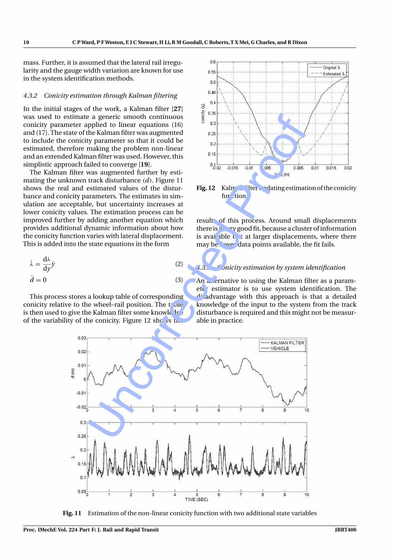
This process stores a lookup table of correspondingconicity relative to the wheel–rail position. The tableis then used to give the Kalman filter some knowledgeof the variability of the conicity. Figure 12 shows the

Fig. 12 Kalman filter updating estimation of the conicityfunction

results of this process. Around small displacementsthere is a very good fit, because a cluster of informationis available but at larger displacements, where theremay be fewer data points available, the fit fails.

4.3.3 Conicity estimation by system identification

An alternative to using the Kalman filter as a param-eter estimator is to use system identification. Thedisadvantage with this approach is that a detailedknowledge of the input to the system from the trackdisturbance is required and this might not be measur-able in practice.

Fig. 11 Estimation of the non-linear conicity function with two additional state variables


Unco

rrecte

d Pr

oof


If the system can be modelled as a ‘grey box’regression model defined as

y(i) = X T(i)θ + ω(i) (4)

where y is the estimated output variable, X is the vec-Q4tor of regressors, θ is the vector of unknown para-meters, ω are the combined known parameter andregressor terms, and i is the discrete sample number,then the parameter estimate can be obtained usingleast squares estimation [28–30]. Non-linear terms canbe added into the regressor matrix, such as higherorder terms [31] or multiple PCP functions [32]. ThePCP technique is a multi-section smoothing func-tion that enables complex non-linear shapes to beapproximated.

Figure 13 shows the results of using the PCP tech-nique to estimate conicity as a function of relativewheel–rail position applied to the model of equation(18) [23]. There is a very close fit to the non-linearshape of the conicity function. It should be noted thatthe conicity may in practice be discontinuous andtherefore not so well matched when using the smoothPCP technique.

4.3.4 Contact geometry estimation by systemidentification

When the identification technique of the previoussection was applied to the non-linear model of equa-tions (11) and (12), the conicity estimates were of poorquality, due to the estimation model being insuffi-cient to fit to the complex dynamics of the simulationmodel. An alternative approach is to estimate therolling radii and contact angles directly.

The unknown non-linear parameters present inthe system equations are the four geometric com-binations (rL + rR), (δL + δR), and (δL − δR). P8 wheelprofiles and 113A railhead shapes in various states

Fig. 13 Least squares estimated conicity function withPCP function

of wear were used for the study. Due to the com-plex discontinuous non-linear nature of these com-binations, a piecewise linear approach was adoptedrather than attempting to fit parameters across theentire range of lateral displacement. To achieve this,the collected dynamic data are first separated into anumber of discrete sections that represent a restrictedrange of the relative wheel–rail displacement. Indi-vidual identifications are performed on each of thesesections.

It was also appreciated that the input from the trackdisturbance should not be modelled as an idealizedsource [33], as this would have different frequencycontent to that found in a real system. Considerationwas also given to the gauge width variation as this addsa degree of uncertainty into the model parameters.Input data used were from the Paddington to Bristolline with lateral disturbance and gauge width variationsampled every 0.2 m by a track recording vehicle. Thestandard deviation of the track disturbance and gaugewidth variation are of similar magnitudes at approx-imately 2 mm. Figure 14 shows (rL + rR) generatedduring simulation, demonstrating that the parametersbeing identified are distributed over a region ratherthan being a single-valued function of lateral displace-ment. This is because the gauge width variation addsuncertainty to the relationship. The gauge width vari-ation also excites the system dynamically, becauseof the asymmetry of the wheelset tread shapes used,though this is a secondary effect.

In practice, for real-time applications, the leastsquares algorithm from the previous section can berun recursively in a similar manner to a Kalman filter.The method potentially saves computation expense,because the calculation is not dealing with the entiredataset for each iteration, just the latest data. Thismakes it feasible for applications where the processingpower may be limited.

Fig. 14 Uncertainty in the parameters due to gaugewidth variation in simulation


Unco

rrecte

d Pr

oof


Two ‘grey box’ multiple input single outputidentifications are performed, where for the lateralacceleration equation, from equation (11)

�1 =[(

−2f22

mv− fy

m

)y +

(−ky

m

)y +

(fy

m

)ym

+(

ky

m

)ym +

(−2f23

mv

)ψ +

(−W

m

)ϕ

](5)

X1 = [ψ , ϕ, 1] (6)

and for the yaw acceleration equation, from equation(12)

�2 =[(

−2f23

Iv

)y +

(−2l2f11

Iv− 2f33

Iv− fψ

I

)ψ

](7)

X2 = [ψ , ϕ, 1] (8)

Figure 15 shows the estimates when the gauge widthvariation is fixed at zero for (rL + rR) and indicatesgood parameter convergence. Figure 16 shows the esti-mates with gauge width variation present. There issome spreading of the estimates because of the gaugewidth variation. Although not shown, the estimates of(δL + δR) fail to converge. The failure to converge maybe due to this parameter being most closely relatedto the variation in gauge width, which is no longerzero.


This section covered a number of methods for thereal-time estimation of critical components associ-ated with the bogie. The first concept was a particlefilter method for the estimation of suspension compo-nents. This showed that a reduced sensor set, on thebogie and the body, could be used to estimate damper

Fig. 15 Recursive least squares estimate of the rollingradii sums with no gauge width variation

Fig. 16 Recursive least squares estimate of the rollingradii sums with gauge width variation

coefficients, but was unable to estimate the effectiveconicity. This was demonstrated with real data col-lected from a Class 175 train. The next step is to applythis technique in real time to a suspension parameterestimation problem.

The second concept was a method for estimatingwheel–rail adhesion using a Kalman filter. Simulationsshowed that, in principle, very low-adhesion condi-tions can be detected. This technique will be appliedto a real system in the future.

The final concept was estimation of the wheel–railprofile. Kalman filtering and non-linear identificationwere applied to the conicity estimation problem. Apiecewise-linear identification was also applied to thedirect estimation of the contact geometry. All the tech-niques demonstrated the potential of the concept,with the main disadvantage being that the distur-bance input from the rail is required, and that this maybe difficult to measure. Possible alternative solutionsfor this are a combined state/parameter estimationloop to first estimate the disturbance, or the use offrequency analysis of output signals along a knownsection of track, both of which are currently beinginvestigated.

5 VEHICLE SPEED MONITORING

The speed of a railway vehicle is normally measuredthrough the use of inductive sensors detecting theteeth of a gearbox or slots of a slotted wheel [34].However, significant problems arise when the con-ditions cannot be satisfied. When wheel slip/slideoccurs (e.g. due to excessive tractive effort and/orextremely low adhesion, the measurement becomesunreliable as large errors may be introduced fromthe wheel slip/slide regardless how accurate the mea-surement of the wheel speed is due to the much


Unco

rrecte

d Pr

oof


increased speed difference between the axle and thevehicle). The use of unbraked and unpowered axlecan solve the problem, but is not always desirableas the reduction on the number of axles for tractionand/or braking may compromise the train control inlow-adhesion conditions. Also, the tachometry-basedtechnique requires regular re-calibration as the wheeldiameter is reduced due to wear. It is also worthnoting that the new technique could be used inconjunction with tachometry to avoid the need forre-calibration.

Although a number of new methods have been pro-posed, most noticeably those based on spatial mea-surement/filtering using sensing technologies such asDoppler radar [35], Eddy current sensors [36], andimage processing [37], those have not been appliedfor traction and braking control applications becausethe measurement accuracy and reliability achievableare not considered sufficient.

5.1 Speed measurement using bogie-basedinertial sensors

The idea for monitoring vehicle speed included inthis article was first proposed in 2008 [38, 39] andwas followed by more detailed studies that tacklespecific technical issues [40, 41]. The new conceptwas conceived from the observation that the absolutevehicle speed determines the time delay in bouncemotion between any two wheelsets as all railwaywheelsets travel on and pass any point of a trackone after another. The time delay in the wheelsetmotions in response to the track irregularities if/whendetected can therefore be used to determine the vehi-cle speed. The measurement can be highly accurateif the speed does not change rapidly and/or the timerequired to detect the delays is sufficiently small notto introduce significant errors in rapid acceleration ordeceleration.

A measurement scheme that takes into consider-ation the practical requirements of the rail industrywas proposed as illustrated in Fig. 17. The need forthe installation of any sensors on the wheelsets/axleboxes, which presents a harsh working environ-ment for sensors, is removed. This is replaced byusing inertial sensors mounted on a bogie frame,which is preferred because the reliability require-ment and also the cost of the sensors will bemuch lower compared with axle-mounted ones. Anintelligent data processing method is then devel-oped to derive (or estimate) the wheelset bouncemotions from the measured bogie bounce and pitchvibrations. The data processing is made as sim-ple as possible to reduce potential difficulties inpractical implementation, but sufficiently effectiveto obtain the estimation of the wheelset motionssuitable for detecting time delays between them

Fig. 17 Speed measurement scheme

[38]. The detection of the time shift is achievedby computing the cross-correlations of the two fil-tered signals and detecting the time shift at thepeak correlation value. It is then straightforward tocalculate the vehicle speed (Vm) from the detectedtime delay (Tdelay) and semi wheel space (Lb) usingequation (9)

Vm = 2Lb

Tdelay(9)

5.2 Measurement performance

As the proposed technique is independent from thewheel rotational speed of the wheels/wheelsets, themeasurement is not affected by wheel slip/slide andit does not require knowledge of wheel radius. Thereis also a clear advantage of the low sensing require-ment. The use of inertial sensors on the bogies can beexpected to become standard installations in futurerailway vehicles, not least as required for tilting con-trol systems, so that there is little extra cost involvedfor practical implementation of the technique. Themeasurement technique is also tolerant to sensorerrors (e.g. the effect of sensor noise tends to be fil-tered out by the cross-correlation computations as thenoise components are uncorrelated between differentsignals [40]).

A moving window of sampled data for cross-correlation calculations as illustrated in equation (2)will enable the continuous detection and update ofthe train speed and is used in the study for perfor-mance assessment. The number of shifted intervals mis incremented from −N to N , where N is the totalnumber of sampled data used for each time window(Twdw = N ∗ Ts) of the running cross-correlation

Rxy(m) =N−m∑

i=1

x(i + m)y(i) (10)


Unco

rrecte

d Pr

oof


Fig. 18 Detected vehicle speed on a low-speed curve

In each computation step (for each time window),the detection of the peak point of cross-correlationsand the corresponding delay intervals will be carriedout which is in turn used to calculate the speed (Vm).Repeating the computation steps, as the time win-dow moves, provides a regular and fast update of themeasured speed signal at the rate of the samplinginterval (Ts).

There are two factors that may potentially affect theaccuracy of the scheme. One is the truncation errorintroduced due to the finite sampling rate for collect-ing/processing data, and the other is due to a delayin the speed detection during vehicle acceleration ordeceleration. However, the use of reasonably selectedsampling rate and data length for the new measure-ment technique will be able to deliver a high level ofperformance as illustrated in the two examples givenbelow.

Figure 18 shows the estimated speed of the pro-posed measurement method, where a comprehensivevehicle model for a conventional bogie vehicle in amulti-body simulation package (Vampire) environ-ment is run at the two different speeds of 50 km/h and100 km/h on a track profile that includes track irregu-larities superimposed on a low-speed curve consistingof a constant curve section of 400 m in curve radius and6◦ in cant angle connected to a straight track sectionvia a transition at either end. Curved tracks presentone of the most difficult conditions for the proposedmeasurement scheme, as there will be variations in thewheel space (increased between the outer wheels anddecreased for the inner wheels).

The measurement for the vehicle speed of 50 km/hvaries within a small range of the real speed and themaximum measurement error is 0.22 km/h. The mea-surement for the speed of 100 km/h gives also a smallerror range with a maximum error of 0.65 km/h. Themeasurement errors here are largely due to the trun-cation caused by the discrete time processing. In thiscase, a sampling interval of 1 ms is used. For the wheelspace of 2.6 m for the vehicle used in this study, the

Fig. 19 Detected vehicle speed during vehicle accelera-tion

truncation errors are expected to be within [−0.22,+0.05 km/h] at the vehicle speed 50 km/h and [−0.57,+0.65 km/h] at the speed of 100 km/h, which are con-firmed by the simulation results. It is possible to reducethe error further by using a smaller sampling interval,but this would have to be balanced with the increasedcomputational demand [41].

Figure 19 shows the second type of error in the formof a measurement delay when the vehicle accelerates(from 40 to 48 m/s, or from 144 to 172.8 km/h) at therate of 1 m/s2, where the truncation error (in a ran-dom manner) is superimposed with a steady stateerror (or offset) due to the delay. This is because thecross-correlation technique detects the average timeshift between the two signals for a given time win-dow and therefore is likely to cause a measurementerror during acceleration or deceleration. This typeof error tends to be more significant at low speeds,as longer time windows are required to provide anaccurate measurement of the time shift [38].


Reliable and accurate measurement of the vehicleground speed even in adverse conditions such aswheel slip/slide does not have to be achieved throughthe expensive equipment and/or complex systems. Itis possible to provide an effective solution with aninnovative use of inertial sensors as demonstratedin this study, even though this type of sensors is notnormally associated with speed measurement. Theperformance of the new measurement method canbe substantially better than the requirement specifiedin the UIC standard for wheel slide control (UIC- Q55014-05) [40]. Possible applications for the proposedmeasurement solution include.

1. Replacement or supplement of the conventionalaxle-based speed sensors to provide more accurate


Unco

rrecte

d Pr

oof


measurement for traction/braking control systemsin all operation conditions including wheel slipor slide.

2. A tool for accurate calibration of the axle-basedsensors, the accuracy of which is affected by thechanges in wheel contact radius due to wear/re-profiling, etc.

3. It can be particularly useful in conditions such astunnels and underground where the use of otherdevices (e.g. GPS) may be problematic.

6 CONCLUSIONS–TRENDS, OPPORTUNITIES,AND RESEARCH CHALLENGES

The article has illustrated potential monitoring oppor-tunities arising from advanced processing of vehicle-mounted sensors: two applications relate to conditionmonitoring of both track and vehicles for enhancedmaintenance and/or improved system reliability, anda third provides operational information for use onboard the train in real time.

The emphasis has very much been upon developingthe processing concepts and the associated algo-rithms, but it is of course necessary to convert the con-cepts into practical engineering solutions, principallyinvolving (i) identification of minimized sensor con-figurations for lower cost and (ii) high-reliability solu-tions to ensure consistently verifiable information.The second point is particularly important, becausewithout good-quality, reliable information the systemwill be difficult to validate where system integrity isinvolved, and may also be discredited where it is usedto inform maintenance processes.

As the title implies, the article has strongly focusedupon the on-train sensing and processing aspects,but one of the key issues that must be addressedprior to the deployment of practical condition mon-itoring systems is the management of data once itleaves the vehicle, in particular because the collec-tion of in-service data will inevitably lead to the needto retain large quantities of data. Data need to beretained and processed in a number of different ways,ideally together with the context of how, when, andwhere they were collected. Initially it is importantthat the data are verified to ensure that they are cor-rect and no sensor errors are present (off-set faults,noise, null values, communication errors, etc.). Sec-ondly, straightforward robust algorithms need to beused to ensure that critical faults are identified in closeto real-time. Thirdly, the data need to be stored forpost-processing (the main focus of this article) to iden-tify longer-term incipient faults. As confidence growsin the accuracy of condition monitoring algorithmsit will not be necessary to retain data for long peri-ods of time. As more data are collected from bothinfrastructure and vehicle-borne sensors, the railwayindustry needs to address the need for standards

for data collection, such standards need to addressthe relationship between data collection by variousmeans.

It is inevitable that condition monitoring technol-ogy will increasingly take advantage of new pro-cessing techniques as they emerge, both to extracthigher-integrity information from existing sets ofsensors and to provide lower-cost solutions usingsimpler, more robust sensor sets. It is thereforeimportant to maintain a ‘watching brief’ on suchtheoretical developments, the challenge being toidentify these possibilities, research their applica-tion within railway systems, and critically evaluatetheir prospective contributions from a business view-point.

ACKNOWLEDGEMENTS

The authors would like to express thanks to the fol-lowing organisations that made this work possible:Rail Research United Kingdom (RRUK), Engineeringand Physical Science Research Council (EPSRC), Tyne& Wear Metro, Alstom, Merseyrail, Department forTransport (DfT) and the Rail Technology Unit (RTU)at Manchester Metropolitan University (MMU).

© Authors 2010

REFERENCES

1 Roberts, C. and Goodall, R. M. Strategies and techniquesfor safety and performance monitoring on railways. InProceedings of the Seventh IFAC Symposium on FaultDetection, Supervision and Safety of Technical Processes,SAFEPROCESS’09, Barcelona, Spain, 30 June–3 July 2009,pp. 746–755.

2 Foeillet, G. IRIS 320 is a global concept inspection vehiclemerging engineering and R&D tools for infrastructuremaintenance. In Proceedings of the EightWorld Congresson Railway research, Seoul, South Korea, 18–22 May 2008.

3 Prendergast, K. Condition monitoring on the Class 390Pendolino. In Proceedings of the Fourth IET Interna-tional Conference on Railway condition monitoring,Derby, UK, 18–20 June 2008.

4 Provost, M. Beyond condition monitoring: from data tobusiness value. In Proceedings of the Fourth IET Inter-national Conference on Railway condition monitoring,Derby, UK, 18–20 June 2008.

5 Burchell, A. K. and Green, S. R. Improving fleet perfor-mance by automatic analysis of enhanced ‘black box’OTMR data. In Proceedings of the Fourth IET Inter-national Conference on Railway condition monitoring,Derby, UK, 18–20 June 2008.

6 Nicks, S. Condition monitoring of the train/track inter-face. In Proceedings of the IEEE Seminar – ConditionMonitoring for Rail Transport Systems, 1998, pp. 7/1–7/6. Q6

7 Ackroyd, P., Angelo, S., Nejikovsky, B., and Stevens,J. Remote ride quality monitoring of Acela train set


Unco

rrecte

d Pr

oof


performance. In Proceedings of the 2002 ASME/IEEEJoint Rail Conference, Washington, DC, 23–25 April 2002.

8 Grassie, S. L. Measurement of railhead longitudinalprofiles: a comparison of different techniques. Wear,1996, 191, 245–251.

9 McAnaw, H. E. The system that measures the system.NDT&E, 2003, 36, 169–179.

10 Weston, P. F., Ling, C. S., Roberts, C., Goodman, C. J., Li,P., and Goodall, R. M. Monitoring vertical track irreg-ularity from in-service railway vehicles. Proc. IMechE,Part F: J. Rail and Rapid Transit, 2007, 221(1), 75–88.DOI: 10.1243/0954409JRRT65.

11 Weston, P. F., Ling, C. S., Roberts, C., Goodman, C. J.,Li, P., and Goodall, R. M. Monitoring lateral track irreg-ularity from in-service railway vehicles. Proc. IMechE,Part F: J. Rail and Rapid Transit, 2007, 221(1), 89–100.DOI: 10.1243/0954409JRRT64.

12 Goodman, C. J., Ling, C. S., Li, P., Weston, P., Goodall,R., and Roberts, C. Condition monitoring of railwaytrack and vehicle suspension using an in-service train.In Proceedings of the IEE International Conference onRailway engineering, Hong Kong and Shenzen, China,15–17 March 2005.

13 Weston, P., Roberts, C., Goodman, C. J., Goodall, R.M., Li, P., and Ling, C. S. Enhanced rail contribu-tion by increased reliability (ERCIR) – instrumentingin-service rail vehicle to monitor vehicle and track. InProceedings of the World Congress on Railway researchWCRR2003, Edinburgh, Scotland, 28 September–1October 2003.

14 Sunder, R., Kolbasseff, A., Kieninger, A., Rohm, A., andWalter, J. Operational experiences with onboard diag-nosis system for high speed trains. In Proceedings ofthe World Congress on Railway Research WCRR2001,Cologne, Germany, 25–29 November 2001.

15 Li, P. and Goodall, R. Model-based condition monitoringfor railway vehicle systems. In Proceedings of the UKACCInternational Conference on Control, University of Bath,UK, 7–10 September 2004, ID-058.

16 Li, P., Goodall, R., Weston, P., Ling, C. S., Goodman, C.,and Roberts, C. Estimation of railway vehicle suspen-sion parameters for condition monitoring. Control EngngPract., 2007, 15, 43–55.

17 Li, P., Goodall, R., and Kadirkamanathan, C. Parame-ter estimation of railway vehicle dynamic model usingRao-Blackwellised particle filter. In Proceedings of theSeventh European Control Conference, Cambridge, UK,1–4 September 2003.

18 Li, P., Goodall, R., and Kadirkamanathan, C. Estimationof parameters in a linear state space model using a Rao-Blackwellised particle filter. IEE Proc. – Control TheoryAppl., 2004, 151(6), 727–738.

19 Charles, G., Goodall, R., and Dixon, R. Model-based con-dition monitoring at the wheel-rail interface.Vehicle Syst.Dyn., 2008, 46(Supplement), 415–430.

20 Polach, O. Creep forces in simulation of tractionvehicles running on adhesion limit. Wear, 2005, 258,992–1000.

21 Pearce, T. G. and Rose, K. A. Measured force-creepagerelationships and their use in vehicle response calcula-tions. In Proceedings of the IAVSD Ninth Symposium,Linkoping, 24–28 June 1985.

22 Harrison, H., McCanney, T., and Cotter, J. Recent devel-opments in coefficient of friction measurements at therail/wheel interface. Wear, 2002, 253, 114–123.

23 Charles, G., Goodall, R., and Dixon, R. A least meansquared approach to wheel-rail profile estimation. InProceedings of the Fourth IET International Conferenceon Railway condition monitoring, Derby, UK, 18–20 June2008.

24 Charles, G., Dixon, R., and Goodall, R. Condition mon-itoring approaches to estimating wheel-rail profiles. InProceedings of the UKACC International Conference onControl, Manchester, UK, 2–4 September 2008, Th05.05.

25 Garg, V. K. and Dukkipati, R. V. Dynamics of railway Q7vehicle systems, 1st edition, 1984 (Academic Press).

26 Wickens, A. H. Fundamentals of rail vehicle dynam-ics: guidance and stability, 1st edition, 2003 (Swets andZeitlinger). Q7

27 Kalman, R. E. A new approach to linear filteringand prediction. Trans. ASME – J. Basic Engng, 1960,35–45. Q8

28 Söderstrom, T. and Stoica, P. System identification, 1989(Prentice Hall). Q7

29 Ljung, L. System identification theory for the user, 2ndedition, 1999 (Prentice Hall). Q7

30 Aström, K. J. Adaptive control, 1989 (Addison-Wesley). Q731 Seber, G. A. F. and Wild, C. J. Nonlinear regression, 2003

(Wiley). Q7

32 Ichida, K., Yoshimoto, F., and Kiyono, T. Curve fittingby a piecewise cubic polynomial. Computing, 1976, 16,329–338.

33 Evans, J. and Berg, M. Challenges in simulation of railvehicle dynamics. Vehicle Syst. Dyn., 2009, 47(8), 1023–1048.

34 Kumagai, N., Uchida, S., Hasegawa, I., and Watanabe, K.Wheel slip rate control using synchronised speed pulsecomputing. In Proceedings of the Seventh InternationalConference on Computers in railways (CompRail 2000),Bologna, Italy, 11–13 September 2000.

35 Badmann, R. Measuring vehicle ground speed with aradar sensor. Sensors, 1996, 13(12), 30–31.

36 Engelberg, T. and Mesch, F. Eddy current sensor sys-tem for non-contact speed and distance measurementof rail vehicles. In Proceedings of the Seventh Interna-tional Conference on Computers in railways (CompRail2000), Bologna, Italy, 11–13 September 2000.

37 Harvey, A. and Cohen, H. Vehicle speed measurementusing an imaging method. In Proceedings of the Interna-tional Conference on Industrial electronics, control andinstrumentation, Kobe, Japan, 28 October–1 November1991.

38 Mei, T. X. and Li, H. Measurement of vehicle groundspeed using bogie based inertial sensors. Proc. IMechE,Part F: J. Rail and Rapid Transit, 2008, 222(2), 107–116.DOI: 10.1243/09544097JRRT154.

39 Mei, T. X. and Li, H. A novel approach for the measure-ment of absolute train speed. Vehicle System Dynamics,2008, 46(Suppl.), 705–715.

40 Mesi, T. X. and Li, H. Monitoring train speed using bogiemounted sensors – accuracy and robustness. In Pro-ceedings of the Fourth IET International Conference onRailway condition monitoring, Derby, UK, 18–20 June2008.


Unco

rrecte

d Pr

oof


41 Mei, T. X. and Li, H. Measurement of vehicle groundspeed with inertia sensors – computation issues. InProceedings of the Eleventh International Conferenceon Computer system design and operations in the rail-way and other transit systems (CompRail 2008), Toledo,Spain, 15–17 September 2008.

APPENDIX 1

Notation

d lateral track displacement (m)fy lateral damper coefficient (Nm2)fψ yaw damper coefficient (Nms)Fs lateral suspension force (N)f11 longitudinal creep coefficient (N)f22 lateral creep coefficient (N)f23 lateral/spin creep coefficient (Nm)f33 longitudinal creep coefficient (Nm2)

g track gauge width (m)I wheelset yaw inertia (kgm2)Iwy wheelset roll inertia (kgm2)ky lateral suspension stiffness (N/m)kψ yaw suspension stiffness (Nm)l half wheelset width (m)m wheelset mass (kg)mm suspended mass (kg)Lb semi wheel spacing (m)Ms suspension moment (Nm)N total number of sampled datar0 nominal rolling radius (m)rL left rolling radius (m)rR right rolling radius (m)Rxy running cross correlationTdelay time delay (s)Twdw time window (s)V vehicle speed (m/s)Vm estimated vehicle speed (m/s)W wheelset weight (N)X least squares regressor matrixy lateral displacement (m)y lateral acceleration (m/s2)

y lateral rate (m/s)y least squares estimation output vector

δL left contact angle (rad)δR right contact angle (rad)θ least squares parameter estimate vectorλ wheelset linear conicityϕ wheelset roll rate (rad/s)φ wheelset roll angle (rad)ψ wheelset yaw angle (rad)ψ wheelset yaw acceleration (rad/s2)

ψ wheelset yaw rate (rad/s)� grey box least squares known state and

parameter matrix

APPENDIX 2

A2.1 Monitoring dynamic performancecharacteristics equations

A2.1.1 Non-linear wheelset and suspended mass model

Wheelset lateral dynamics

my + 2f22

V

[y + rL + rR

2ϕ − V ψ

]+ 2f11

[1 − rL + rR

2r0

]ψ

+ 2f23

[ψ

V− δL − δR

2r0

]+ W

[δL − δR

2+ ϕ

]= Fs

(11)

Wheelset yaw dynamics

I ψ + IwyVr0

ϕ + 2l2f11

r0

(rL − rR

2l

)− 2f23

Vy

− f23(rL + rR)

Vϕ + 2f23ψ + 2l2f11

Vψ − f33(δL − δR)

r0

− lW (δL + δR)

2ψ + 2f33

Vψ = Ms (12)

Suspended mass lateral dynamics

y = 1mm

(Fs) (13)

Lateral suspension force

Fs = ky(ym − y) + fy(ym − y) (14)

Suspension yaw moment

Ms = −kψψ − fψψ (15)

A2.2 Full linear equations

Wheelset lateral dynamics

my + 2f22

V

[y + r0

λ

ly − V ψ

]+ 2f23

Vψ + W λ

ly = Fs

(16)


I ψ + IwyV λ

r0ly + 2l2f11λ

r0y − 2f23

V

(y + r0λ

ly − V ψ

)

+ 2l2f11

Vψ − lW λψ + 2f33

Vψ = Ms (17)

A2.3 Simplified linear equation


I ψ + 2l2f11λ

r0y + 2l2f11

Vψ = Ms (18)


Unco

rrecte

d Pr

oof

Documents

Condition monitoring opportunities using vehicle … University Institutional Repository Condition monitoring opportunities using vehicle-based sensors This item was submitted to Loughborough