Condensate Retention Effects on the Air-Side Heat Transfer

Condensate Retention Effects on the Air-Side Heat Transfer Performance of Automotive Evaporator Coils

ACRCCR-32

For additional information:

Air Conditioning and Refrigeration Center University of Illinois Mechanical & Industrial Engineering Dept. 1206 West Green Street Urbana, IL 61801

(217) 333-3115

J. M. Kaiser and A. M. Jacobi

July 2000

The Air Conditioning and Refrigeration Center was founded in 1988 with a grant from the estate of Richard W. Kritzer, the founder of Peerless of America Inc. A State of Illinois Technology Challenge Grant helped build the laboratory facilities. The ACRC receives continuing support from the Richard W. Kritzer Endowment and the National Science Foundation. Thefollowing organizations have also become sponsors of the Center.

Amana Refrigeration, Inc. Ar~elik A. S. Brazeway, Inc. Carrier Corporation Copeland Corporation DaimlerChrysler Corporation Delphi Harrison Thermal Systems Frigidaire Company General Electric Company General Motors Corporation Hill PHOENIX Honeywell, Inc. Hussmann Corporation Hydro Aluminum Adrian, Inc. Indiana Tube Corporation Invensys Climate Controls Lennox International, Inc. Modine Manufacturing Co. Parker Hannifin Corporation Peerless of America, Inc. The Trane Company Thermo King Corporation Valeo, Inc. Visteon Automotive Systems Whirlpool Corporation Wolverine Tube, Inc. York International, Inc.

For additional information:

Air Conditioning & Refrigeration Center Mechanical & Industrial Engineering Dept. University of Illinois 1206 West Green Street Urbana,IL 61801

217 3333115

Abstract

The effect of condensate accumulation and shedding on the air-side thennal

perfonnance of automotive evaporator coils has been studied. Experiments under wet and

dry conditions were conducted to expose the impact of condensate on five different coils.

Condensate retention data were collected in both real-time and at steady-state to

quantitatively detennine how condensate load up on a coil surface. Sensible Colburn j

factors and friction factors were calculated from the experimental data, and the relative

perfonnance of different coils was discussed. A dynamic drainage test was developed to

study the nature of water draining out of a heat exchanger. It was found the simple

drainage test qualitatively predicted how much condensate would be retained by different

coils under operating conditions. Current retention modeling techniques were adapted to

include automotive evaporators.

111

Table of Contents

Page

List of Tables .................................................................................................................... vii

List of Figures .................................................................................................................. viii

Nomenclature ...................................................................................................................... x

Chapter 1 Introduction and Literature Review ................................................................... 1

1.1 Introduction .......................................................................................................... 1

1.2 Literature Review ................................................................................................. 2

1.2.1 Early Studies ........................................................................................... 2

1.2.2 Automotive Evaporator Condensate Drainage and Thermal

Performance ............................................................................................ 7

1.2.3 Modeling Condensate Retention ............................................................ 9

1.3 Objectives .......................................................................................................... 11

Chapter 2 Experimental Apparatus and Methods ............................................................. 12

2.1 Experimental Apparatus ..................................................................................... 12

2.1.1Wind Tunnel .......................................................................................... 12

2.1.2 Condensate Visualization ..................................................................... 16

2.1.3 Dynamic Drainage ................................................................................ 17

2.1.4 Contact Angle Measurements ............................................................... 19

2.1.5 Heat Exchanger Specifications ............................................................. 19

2.2 Experimental Conditions and Procedures .......................................................... 20

2.2.1 Thermal Performance ........................................................................... 20

2.2.2 Steady-state Condensate Retention ...................................................... 20

2.2.3 Real-time Condensate Retention .......................................................... 21


Chapter 3 Results and Discussion ..................................................................................... 30

3.1 Thermal Performance ......................................................................................... 30

3.2 Condensate Retention ........................................................................................ 35

IV

3.2.1 Real-time Retention .............................................................................. 36

3.2.2 Steady-state Retention .......................................................................... 40

3.3 Dynamic Drainage ............................................................................................. 41

Chapter 4 Conclusions and Recommendations ................................................................. 61

4.1 Conclusions ........................................................................................................ 61

4.1.1 Thermal-Hydraulic Performance .......................................................... 61

4.1.2 Condensate Retention ........................................................................... 62


4.2 Design Guidelines .............................................................................................. 63

4.3 Recommendations for Future Studies ................................................................ 65

Appendix A Data Reduction ............................................................................................. 68

A.l Mass Fluxes ....................................................................................................... 68

A.2 Heat Transfer Rates ........................................................................................... 69

A.3 Fin Efficiency .................................................................................................... 69

AA Heat Transfer Coefficients ................................................................................ 72

Appendix B Uncertainty Analysis .................................................................................... 81

B.l Uncertainty in Measured Parameters ................................................................ 81

B.2 Uncertainty in Calculated Values ...................................................................... 82

B.2.1 Tube-side ............................................................................................. 82

A. Heat Transfer Rate ............................................................................... 82

B.2.2 Air-side ................................................................................................ 83

A. Vmax .........•............•....•.......................................................................... 83

B. Reynolds Number ................................................................................. 84

C. Friction Factor ...................................................................................... 84

D. Heat Transfer Coefficient.. ................................................................... 85

E. Sensible j factor .................................................................................... 86

B.3 Uncertainty in Measured Condensate Retention ............................................... 86

BA Uncertainity in Dynamic Drainage Tests .......................................................... 87

Appendix C Condensate Retention Model ....................................................................... 89

v

C.l Prior Work ......................................................................................................... 89

C.2 Adaptations ........................................................................................................ 92

References ......................................................................................................................... 98

VI

List of Tables

Page

Table 2.1 Tested coil descriptions .................................................................................... 29

Table 3.1 Tilt test and vertical test comparison ................................................................ 60

Table A.1 Friction factor and Wilson plot data EES code listing ..................................... 77

Table A.2 j factor EES code listing .................................................................................. 79

Table B.1 Uncertainties in measured parameters ............................................................. 88

Table C.1 Relative surface areas and maximum droplet size constraints for Coil 4 ........ 95

Table C.2 Summary of model results for Coil 4 ............................................................... 96

Table C.3 EES code for computing mass per unit area for different surfaces .................. 97

Vll

List of Figures

Page

Figure 2.1 Horizontal flow wind tunnel. (A) 36-cm diameter round sheet metal duct.

(B) Thermal mixing chamber. (C) Screens and honeycomb flow straighteners.

(D) 9:1 contraction. (E) Test heat exchanger. (F) Inlet/ outlet measurement

sections. (G) Strip resistance heaters. (H) Steam injection tube. (I) Axial

blower. .............................................................................................................. 25

Figure 2.2 Test Section for Wet and Dry Runs. (A) Pressure taps (top and bottom). (B)

Chilled mirror hygrometer sensors. (C) Insulated clear acrylic. (D) Drainage

tray. (E) Thermocouple grid (inlet and outlet) ................................................. 25

Figure 2.3 Air velocity measurement locations ................................................................ 26

Figure 2.4 Closed environment glove box apparatus for examining condensing fin

samples. (A) Beaker with water. (B) Fin stock. (C) Peltier device and liquid

heat exchanger. (D) Glove. (E) Fan ................................................................. 26

Figure 2.5 Dynamic drainage apparatus ........................................................................... 27

Figure 2.6 Attaching mechanism for drainage test coils ................................................... 27

Figure 2.7 Real time retention apparatus. (A) Wind tunnel. (B) Suspension mechanism

components. (C) Balance. (D) Inlet! outlet coolant lines. (E) Test heat

exchanger. (F) Drain ........................................................................................ 28

Figure 2.8 Contact angle measurement apparatus ............................................................ 28

Figure 3.1 Coil 1 air-side sensible heat transfer coefficient versus face velocity ............. 47





Figure 3.6 Coil 1 air-side pressure drop in mm of water versus face velocity ................. 49




Figure 3.10 Coil 5 air-side pressure drop in mm of water versus face velocity ............... 51

V111

Figure 3.11 Coil 1 j and ffactors versus air-side Reynolds number ................................. 52

Figure 3.12 Coil2j and ffactors versus air-side Reynolds number ................................. 52

Figure 3.13 Coil 3 j and f factors versus air-side Reynolds number ................................. 53



Figure 3.16 Real time condensate retention and humidity ratio for Coil 5 versus time ... 54

Figure 3.17 Real time condensate retention repeatability for Coil 4 ................................ 55

Figure 3.18 Real time plot for Coil 4 showing overshoot at higher velocity .................... 55

Figure 3.19 Steady state retention for all coils versus face velocity ................................. 56

Figure 3.20 Steady state retention per unit of heat transfer area versus face velocity ...... 56

Figure 3.21 Drainage test plot for Coil 3 illustrating the repeatability of the

experimental technique .................................................................................... 57

Figure 3.22 Partial plot of the repeatability test results showing the area of maximum

error .................................................................................................................. 57

Figure 3.23 Dynamic test results for the fast draining coils ............................................. 58

Figure 3.24 Dynamic test results for the sustained draining coils .................................... 58

Figure 3.25 Extended time drainage test results ............................................................... 59

Figure 3.26 Comparison plot between a vertical coil and a coil tilted 10° ....................... 59

Figure 3.27 Droplet forces and bridges ............................................................................. 60

Figure A.1 Example of Modified Wilson-plot.. ................................................................ 76

Figure C.1 Forces acting on a droplet on an inclined surface due to gravity,

air-flow, and surface tension ............................................................................ 95

Figure C.2 Measured and predicted values of steady-state condensate retention

for Coil 4 .......................................................................................................... 96

IX

Nomenclature

A area (m2)

Adrop area of a droplet (cm2)

Afr frontal area (m2)

b intercept of least squares fit line

C constant of integration

Cd drag coefficient

Cp specific heat at constant pressure (kJ/kg-K)

D diameter (m)

DAB binary mass diffusion coefficient (m2/s)

Ddrop diameter of droplet (m)

Dh hydraulic diameter (m)

L1PHx heat exchanger differential pressure (kPa)

f friction factor

Is fin spacing (rom)

Fd air drag force (N)

Fg gravitational force (N)

Fs surface tension force (N)

g gravitational acceleration (9.81 m1s2)

G mass velocity based on minimum free flow area (kg/m2 -s)

h enthalpy (kJ/kg)

ho air-side heat transfer coefficient (W/m2-K)

hi coolant-side heat transfer coefficient (W/m2 -K)

hm mass transfer coefficient (kg/m2-s)

j sensible j factor

k thermal conductivity (W/m-K)

Lf length or depth of fin (m)

Le Lewis number

m mass flux (kg/s)

mo fin efficiency parameter

x

Nu Nusselt number

Pr Prandtl number

q heat transfer rate (KW)

R thennal resistance (K/W)

Rc coolant flow meter output (pulse/s)

Re Reynolds number

T temperature (OC)

t time (s)

V velocity (mls)

Greek symbols

a angle of inclination (radians)

8 fin thickness (m)

~ relative humidity

y surface tension (mN/m)

" fin efficiency, surface effectiveness

Il dynamic viscosity (N-s/m2)

8 dimensionless temperature

8A advancing contact angle (radians)

8M mean contact angle (radians)

8R receding contact angle (radians)

p density (kg/m3)

cr contraction ratio (Amini Afr)

Subscripts

air aIr

atm atmospheric pressure (atm)

ave average

c coolant

cali calibrated

dp dewpoint

Xl

dry dry condition

f fin

fr frontal

i tube-side

in inlet

I liquid

mair mean aIr

min minimum

max maXImum

a air-side

out outlet

sens sensible

t total

wet wet condition

XlI

Chapter 1 Introduction and Literature Review

1.1 Introduction

In automotive air-conditioning systems, the air-side surface temperature of the

vapor-compression evaporator is usually below the dew point of the conditioned air, and

it is common for water to condense onto the air-side heat-transfer surface. Condensate

accumulates on the surface and is retained by surface tension until it is removed by either

gravitational or flow forces. Retained condensate plays an important role in the overall

performance of the air-conditioning system; it can profoundly affect the heat transfer and

pressure drop performance, but there is disagreement on the overall impact in some heat

exchanger geometries. Condensate retention also has important implications on air

quality. Condensate that blows off with the conditioned air stream can affect comfort, and

water provides a medium for biological activity on air-handling surfaces. The post

operation (off-cycle) condensate draining behavior is extremely important in this respect,

because the warm, moist conditions prevailing after system shut down are conducive to

biological growth.

The focus of this project was on the effect of condensate on air-side thermal

hydraulic performance, with an overall goal to develop new fin-design guidelines that

maximize performance under dehumidifying conditions. A wind tunnel was designed and

constructed for testing heat exchangers under dry and condensing conditions.

Experiments were conducted to obtain steady state and real-time measurements of

condensate retention. Furthermore, heat transfer and pressure drop data for heat

exchangers under dry and condensing conditions were recorded. Extensive drainage tests

1

were conducted using a dynamic drainage test apparatus. The data from the experiments

were used to aid in development and validation of a retention model.

1.2 Literature Review

The majority of the work on air-side thermal performance under dehumidifying

conditions has concentrated on heat exchangers with round tubes, as opposed to the flat

tube, brazed-plate geometry of this study. Nevertheless, the prior work is helpful in

developing an understanding of the impact of condensate retention and shedding. This

section includes a discussion of past work on flat plates, finned-tube coils with plain and

enhanced fins, and the limited work in the open literature on automotive-style

evaporators. Finally, a discussion of condensate retention, drainage, and modeling is

presented.

1.2.1 Early Studies

Bettanini (1970) performed numerous experiments in heat and mass transfer for a

vertical plate and reported an enhancement in sensible performance under condensing

conditions. Bettanini postulated the effect was caused (in part) by an increase in surface

roughness caused by condensation on the surface. Two types of experiments were

conducted to verify this effect. A soap and water solution was sprayed on the surface to

temporarily cause filmwise condensation, and heat transfer measurements were taken

until the condensation turned to dropwise, thus increasing surface roughness. The

sensible heat transfer coefficient increased by approximately 20% when the condensation

turned to dropwise, supporting the roughness effect idea. Additional experiments were

done using gypsum chips to simulate water droplets on the surface. The results from these

tests showed approximately a 10% increase in performance. While these tests do show an

2

impact from surface roughness, the experimental apparatus and procedure used was

simple and not well controlled (as noted by Bettanini), and the extension of these results

to more complicated heat exchangers and flow regimes is unclear.

Yoshii et al. (1973) examined the effects of dropwise condensation on the

pressure drop and heat transfer performance of wavy-fin heat exchangers. It was found

that pressure drop for wet heat exchangers was 50 to 100% higher than for dry

exchangers. Under wet conditions, a 20 to 40% enhancement in heat transfer coefficient

was found for the heat exchangers. To investigate the effect of condensate on the flow

dynamics, scale-up models of the heat exchangers with simulated condensate were made

and tested in a water channel at similar Reynolds numbers. Y oshii and coworkers

reported that drops on the flat fin surface promoted turbulence when the droplet adhered

on the ridge or valley in the wavy fin, but caused separation when adhered to the area

between bends. Additionally, water bridges between the tube and fins significantly

increased the wake region downstream of the tube, but downstream droplets can direct

flow into the wake region. From these observations Y oshii and coworkers concluded the

overall impact on condensate depends on both location and shape of the droplets.

Guillory and McQuiston (1973) and McQuiston (1976) studied developing flow

between horizontal flat plates and found a heat transfer enhancement of about 30% for

wet surface conditions. In agreement with Bettanini, Guillory and McQuiston explained

that the condensate that formed on the heat exchanger increased the surface roughness of

the exchanger walls and this increased roughness explained the increase in heat transfer

and pressure drop found under wet conditions. Tree and Helmer (1976) also studied a

parallel plate heat exchanger under condensing conditions. Unlike Guillory and

3

McQuiston, they found that condensation did not affect the sensible heat transfer and

pressure drop during laminar flow. However, agreement was found in the transitional and

turbulent regime, where condensate was found to increase heat transfer and pressure drop.

For plain-fin-and-tube geometries, Myers (1967), Elmahdy (1975), and Ekels and Rabas

(1987) have reported a sensible enhancement under wet conditions.

Inconsistent with a simple roughness effect, McQuiston (1978a,b) found the

enhancement in plain finned-tubes to be strongly dependent on fin spacing. For circular

finned tubes, Jacobi and Goldschmidt (1990) found the enhancement to be Reynolds

number dependent. A degradation was observed at low Reynolds numbers, and an

enhancement was found at high Reynolds numbers. Jacobi and Goldschmidt suggested

that their results, and those of McQuiston, were due to condensate retention. At low

Reynolds numbers, retained condensate would occupy heat exchanger area with a

deleterious effect, but at high Reynolds numbers, vapor shear would remove retained

condensate and roughness effects of the remaining condensate would dominate. This

explanation has since been supported by the work ofUv and Sonju (1992).

Further complicating the issue, spatial variations of the dry-surface local heat

transfer coefficient mayor may not have a significant impact on the fin efficiency (Huang

and Shah, 1991; and Kearney and Jacobi, 1996), and the same could be true for a wet fin.

Hu et al. (1994) conducted detailed local heat transfer experiments with simulated

condensate. Their results indicate that for circular fins the effect on fin efficiency is small,

as did Kearney and Jacobi, but the overall impact of condensate retention on average heat

transfer can be significant. For circular fins, the average sensible heat transfer coefficient

4

can be increased by as much as 30% due to condensate effects at high Reynolds numbers.

The impact in other geometries (e.g., louvered fins) remains unclear.

Hong (1996) examined the use of hydrophilic coatings to improve wettability and

thereby decrease the pressure drop associated with wet-fin operation. Wavy, lanced, and

louvered fins were studied, and at fixed face velocity of 2.5 mis, the ratio of wet-to-dry

pressure drop was 1.2 for each geometry tested. A model to predict the carry-over

velocity was developed and compared to experimental data. Carry-over velocity is

dependent on surface tension forces that depend on contact angle. Hong presented contact

angle data obtained from a sessile drop goniometer test; however, because a static test

procedure was adopted, no measure of contact angle hysterisis was obtained-a result

between the advancing and receding is all that can be achieved through such an approach.

Hong found that after approximately 1,000 wetting cycles the coated and uncoated test

surfaces all exhibited contact angles of approximately 60 degrees.

Korte and Jacobi (1997) studied the effects of condensate retention on the air-side

performance of plain-fin-and-tube heat exchangers. Experiments were conducted under

dry conditions and then repeated under condensing conditions. It was found that the heat

transfer performance under condensing conditions was dependent on the fin spacing. An

enhancement in heat transfer for wet conditions was seen for a 6.35 mm fin pitch heat

exchanger but not for a 3.18 mm fin pitch heat exchanger. The results for the heat

exchanger with a 3.18 mm fin pitch showed the heat transfer performance under wet

conditions to sometimes be better and sometimes worse than for dry conditions. It was

also found that the effect of condensation on friction factor was dependent on fin spacing.

Similar friction factors were observed for a 6.35 mm fin pitch heat exchanger under wet

5

and dry conditions. At 3.18 mm fin pitch, there was a significant increase in friction

factor under wet conditions. However, with increasing air-flow rates the quantity of

retained condensate and the increase in friction factor decreased.

Wang et al. (1997) studied the performance of plain finned-tube heat exchangers

under dehumidifying conditions. The effects of fin spacing, number of tube rows, and

inlet conditions were investigated. Nine plain-fin-and tube heat exchangers were tested

with fin spacing ranging from 1.82 mm to 3.2 mm and 2, 4, and 6 tube rows. Heat

transfer performance and friction factors were observed for the exchangers at a relative

humidity of 50% and 90%. The friction factors for wet coils were found to be much

larger than those of dry coils. For fully wet conditions, the friction factors were found to

be 60 to 120% higher than for dry conditions and insensitive to change in inlet air relative

humidity, fin spacing, and the number of tube rows. Sensible j factors under

dehumidifying conditions were not found to be dependent on the inlet air conditions.

Under wet conditions, a degradation in sensible heat transfer was seen at low Reynolds

numbers. At high Reynolds numbers, a small enhancement in heat transfer performance

was observed under wet conditions but the enhancement disappeared as the number of

tube rows increased.

Ha et al. (1999) studied the hydraulic performance of wet fin-and-tube heat

exchangers with various wettability coatings. Contact angle measurements obtained were

used to characterize each ofthe different surfaces. For all surfaces, an increase in pressure

drop was found for heat exchangers under wet conditions. The increase in pressure drop

was greater with increasing contact angles. It was also found that surfaces with smaller

contact angles retained less condensate and required less time to reach a steady value of

6

retained condensate. Furthennore, pressure drop models for dry and wet heat exchangers

with dropwise condensation were developed.

Yin and Jacobi (1999) studied the effect of condensate retention on thennal

perfonnance for plain-fin and wavy-louvered fin heat exchangers exposed to air frontal

velocities from 0.8 mls to 2.0 mls. They reported the amount of condensate was

independent of face velocity for these geometries and air-flow rates, but dependent on fin

geometry and contact angles. A greater amount of condensate was retained in the wavy

louvered coils. Under wet conditions, Colburn j factor decreased, and this degradation

was greater at greater fin densities--consistent with a greater amount of water being

retained. Additionally, under dry conditions, the wavy-louvered had a higher j factor

relative to the plain fin coil, but the enhancement disappeared under wet conditions. The

work of Kim and Jacobi (1999) similarly showed a decrease in thennal perfonnance for

both plain and enhanced fins (slit-fin) round tube evaporators. The increased pressure

drop was concluded to be caused by the blockage effect of retained condensate and the

decrease in wet heat transfer due to fouling of the air-side heat transfer surface in plain

fins, and additional fouling of the louvers or slits by condensate bridging.

1.2.2 Automotive Evaporator Condensate Drainage and Thermal Performance

Little work has been reported in the open literature to address condensate drainage

on automotive-style evaporator coils; however, a few studies addressing the thennal

perfonnance of such coils have been reported. Wang et al. (1994) found an increased air

side heat transfer coefficient under wet conditions and surmised condensate on the fins

acted as an enhancement by increasing surface roughness. Their study included only two

7

different heat exchangers, giving useful but limited results. Osada et al. (1999) performed

heat transfer and visualization experiments on single fin columns of flat tube evaporators.

They investigated the effects of surface wettability, louver geometry, and inclination

angle on condensate drainage. Osada and co-workers concluded that fin surface

characteristics near the air-flow-exit face of the heat exchanger were an important factor

in condensate drainage. This region of the fin is important because airflow forces push

condensate toward that part of the fin-it accumulates there until it is drained by gravity.

Osada and co-workers found that decreasing the non-louvered length on the fin promotes

better drainage; they suggest that increasing the louver cut length decreases the amount of

louver blockage caused by condensate bridging within the inter-louver space.

Very recently, McLaughlin and Webb (2000a) studied the impact of fin geometry

on drainage characteristics and retention using a table-top test cell for experiments with a

single-fin column. They undertook several methods to validate their test methods, and

they argued that this approach with a single fin specimen provides results representative

of a full-scale heat exchanger. Single-fin tests were conducted with an air flow of 2.5m1s

and an entering relative humidity greater than 95%. During these experiments, tube-side

cooling was provided by cold water circulated through a tube brazed to one side of the

fin. This simplification allowed optical access through glass on the other side of the fin,

but it certainly compromised the thermal boundary conditions, and the fin-glass interface

modified the geometry and surface tension boundary conditions on retained condensate

as recognized by McLaughlin and Webb. Their results suggest louver pitch is the single

most important parameter determining drainage characteristics of louver fin evaporators.

They state that a critical louver pitch between 1.1 mm and 1.3 mm exists for a louver

8

angle of 30°, where condensate retention increases by 26%. In a related study, they found

up to a 40% decrease in air-side heat transfer coefficient under wet conditions for the 1.1-

mm-Iouver-pitch evaporator, no change under wet conditions for the 1.33-louver-pitch

coil (McLaughlin and Webb, 2000b). They conclude that condensate bridging within the

louvers is responsible for the increase in retention and degradation of perfonnance.

1.2.3 Modeling Condensate Retention

Several models of condensate retention have been proposed. Rudy and Webb

(1981) reported a method for measuring condensate retention for the condensation of pure

fluids on integral low-finned tubes. They found that condensate retention was intensified

for a close fin spacing and suggested that the gravity-drained model of Beatty and Katz

(1948) was inadequate because it neglected surface tension effects; they later developed

their own models (Webb, et aI., 1985a,b). Unfortunately, there is little hope of

generalizing these geometrically specific results. Jacobi and Goldschmidt (1990)

presented a simplified model of condensate retention in the "bridges" fonned between

neighboring fins. Their model was qualitatively successful in predicting heat transfer

effects; unfortunately, it is not possible to trivially generalize this model for other

condensate geometries or more complex fins.

Korte and Jacobi· (1997) developed a model to predict the quantity of retained

condensate for uncoated aluminum plain-fin-and-tube heat exchangers with a fin spacing

of 6.35 mm. The quantity of retained condensate was detennined by calculating the

volume of retained condensate and multiplying this volume by the density of the water.

Unlike previous studies, the model incorporated advancing and receding contact angles

9

that were used to detennine surface tension forces. Modeling techniques were relatively

successful in predicting the quantity of retained condensate for the 6.35 mm fin pitch heat

exchanger, but many higher order effects were not included. The model of Korte and

Jacobi incorporated only droplets adhering to the surface, other features such as bridges

occurring between fins, fillets and bridges at the fin-tube junction, or other condensate

geometries were not included. However, they developed initial force balances to assist in

detennining the sizes of some simple bridges. The droplet size distributions used in the

model were based on the work of Graham (1969). Air-flow forces were included by

assuming a constant drag coefficient and approximating the local velocity using laminar

flow approximations. Gross surface coverage values were estimated from experimental

observations and, as noted by Korte and Jacobi, there may be variations in area covered

through the length of the fin due to sweeping effects.

The retention model of Korte and Jacobi was adapted to include condensate

bridging at the fin-tube junction by Yin and Jacobi (1999). Furthennore, the modeling

technique was applied to a heat exchanger with over twice the fin density. The decreased

fin spacing made it difficult to detennine the droplet size distributions on the heat

exchanger. Therefore, a stock fin sample was studied in the controlled environment of a

glove box. Using image analysis software, Yin and Jacobi detennined not only the

droplet size distribution (still based on the concepts developed by Graham), but also

investigated the vertical variations of droplet size density due to sweeping along the fin.

The model successfully predicted the amount of condensate retention in a 2.13 mm fin

pitch coil, but over predicted the mass in heat exchangers with 1.59 mm and 1.27 fin

pitches. This discrepancy was attributed to the assumption in the model of zero

10

interaction between droplets on adjacent fins. It is likely that in a heat exchanger with

tighter fin spacing for two droplets on adjacent fins would coalesce, creating a fin bridge,

and cause a greater sweeping effect as the larger fin bridge is shed. A similar approach in

modeling was studied by Kim and Jacobi (1999), and a corresponding over-prediction of

mass as heat exchanger geometry became more complex was reported.

1.3 Objectives

The objectives of this project were to determine the effect of condensate retention

on air-side heat transfer performance of automotive evaporator coils, to investigate the

drainage characteristics during operation and after system shutdown, and finally to

develop a condensate retention model to predict the amount of condensate retention based

on prior modeling efforts for plain-fin-and-tube heat exchangers. Air-side heat transfer

performance under and condensing conditions were measured, and condensate retention

measurements were taken in real-time and at steady state. A dynamic drainage test rig

was developed and the results were used to aid in the understanding of retention and

shedding of condensate. A model was developed to predict total condensate retention

under normal operating conditions.

11

Chapter 2 Experimental Apparatus and Methods

A closed-loop wind tunnel was designed and constructed for testing heat

exchangers under condensing conditions. Heat exchanger perfonnance and condensate

retention measurements were obtained using the apparatus. A condensate visualization

chamber was built to study retention on small pieces of fin stock. A water drainage test

apparatus was constructed to test drainage behavior of heat exchangers. This chapter

describes the experimental apparatus, instruments, experimental procedures, and heat

exchangers tested for this research.

2.1 Experimental Apparatus

2.1.1 Wind Tunnel

The thennal perfonnance and condensate retention apparatus consisted of a

closed-loop wind tunnel, a test section for testing heat exchangers exposed to horizontal

air-flow, and a coolant loop that circulates a single-phase coolant. The wind tunnel is

shown schematically in Figure 2.1. It was used to obtain measurements of retained

condensate and heat transfer perfonnance for various types of heat exchanger geometries.

Experiments were conducted with a horizontal flow of air, and specimens were tested at

various air flow rates typical to mobile air-conditioning applications. The closed-loop

wind tunnel allowed control of temperature, humidity, and air flow rate. Air temperature

was controlled by varying the power supplied to ten electrical resistance heaters using a

PID controller; the total capacity of these heaters was 7.5 kW. A feedback Type-K

thennocouple was located just downstream of the main tunnel contraction. The heaters

were located in two banks, one upstream of the blower and the other downstream of the

blower. The second bank was used only during testing at the highest heat duties. Evenly

12

spaced Type-T thennocouples were used both upstream and downstream of the test

section to measure the inlet and outlet air temperature. A six-thennocouple grid was used

upstream and a twelve-thennocouple grid was used downstream to measure the average

inlet and outlet air temperatures. The upstream temperature readings for all

thennocouples varied from the mean less than O.8°C at the lowest air velocity and less

than O.3°C at the highest velocity, with the upper row always reading higher than the

lower row. The relatively large variation at the low flow rates was caused by improper

mixing in the thennal-mixing chamber. The upper duct discharged directly into the top of

the chamber and caused excessive stratification. Each thennocouple was individually

referenced to a thennocouple located in an ice bath, and calibrated to a NIST traceable

mercury-in-glass thennometer using a thennostatic bath. Calibration data were fit with

fifth order polynomials for each thennocouple. The dewpoints of the air were measured

by chilled mirror hygrometers with a measurement uncertainty of ±O.2°C. Air was

supplied to the chilled mirrors through sampling tubes located 30-cm upstream and

downstream of the test section. A small, medical diaphragm air pump drew air through

the sampling tubes. The dewpoint of the incoming air was maintained using a steam

injection system. The humidifier was a boiler capable of providing 11.5 kglhr of steam.

The output of the humidifier was controlled by varying the input heater power using a

PID controller. The upstream dewpoint monitor provided the control signal for the steam

injector. The steam was injected into the tunnel through a perforated pipe 50-cm

downstream of the first bank of heaters. An axial fan, belt driven by a DC motor, mixed

the airstream and provided volumetric flow rates up to 8.5 m3/min. Upstream of the test

section, air was drawn from a thennal mixing chamber and passed through a set of

13

screens, honeycomb flow straighteners, and a 9: 1 contraction to obtain steady laminar

flow before passing through the test section. Additional, smaller contractions were

required just upstream of the test coil to match the flow to each geometry. These elliptical

contractions were cut from Styrofoam, covered with aluminum tape, and attached to the

wind tunnel walls with adhesive.

The test section, shown In Figure 2.2, was designed for testing wet heat

exchangers. The design allowed for both real-time and steady-state measurements of the

mass of retained condensate. The test section was constructed using clear acrylic to allow

for optical access. In order to limit conduction losses when observations were not being

made, the test section was insulated with 1.27 cm thick polyethylene foam insulation with

an insulation factor of 0.08 W/m2K. Upstream and downstream pressure taps were

located on the upper and lower walls of the rectangular test section for measuring the

pressure drop across the heat exchanger. The pressure taps were located approximately

7.5 cm upstream and downstream of the heat exchanger, with two taps at each location

spaced 7.5 em apart centered on each side of the test section. An electric manometer with

an uncertainty of ±0.124 Pa was used to measure the air-side pressure drop across the

heat exchanger. Face velocities were measured at the test section using a constant

temperature thermal anemometer. The face velocity was determined by taking twelve

equally spaced measurements traversing the height of the heat exchanger in three places

at each of the four velocity measurement locations shown in Figure 2.3. The twelve

measurements were recorded and an average face velocity was determined. The velocity

measurements were within 11 % of the average at the lowest velocity and 8% at the

highest velocity. Turbulence intensity measurements were taken using a hot wire

14

anemometer at the velocity measurement locations, with a plain-fin-and-tube installed in

the test section. Measurements were made at three locations and except for the small

wake region behind the thermocouples, the turbulence intensity was less than 2.5%.

A single-phase ethylene glycol (DOWTHERM 4000) and water mixture was

circulated on the tube side of the heat exchanger. Over the course of this project, two

different concentrations of ethylene glycol were used, 32.6% and 40.0%. The

concentrations were mixed and maintained by measuring the specific gravity of the

mixture using a NIST traceable hydrometer. The required specific gravity was obtained

by interpolating on manufacturer provided tables. Coolant-side temperatures were

measured using type-T immersion thermocouples located approximately two meters

upstream and downstream of the heat exchanger. Each thermocouple was individually

referenced to a thermocouple located in an ice bath, and calibrated in the same manner as

the wind tunnel grid thermocouples. An R-502 liquid-to-liquid, variable-speed chiller was

used to control the coolant temperature. Temperature of the solution was controlled using

an immersion temperature probe on the supply line as the control signal for a proportional

controller driving the compressor. The mixture was circulated through a copper tubing

loop by two pumps. An integral, centrifugal, recirculation pump provided a 200-kPa head

to a positive displacement rotary gear pump. The gear pump was belt driven to minimize

vibrations by a two horsepower motor. The coolant flow was controlled by using an

inverter to vary the drive motor speed. The test heat exchanger was connected to the

copper tubing with flexible, reinforced, PVC tubing that terminated with quick

disconnect couplings to facilitate removal of the coil. All tubing was insulated with 9.5

mm polyethylene foam insulation with an insulation factor of 0.05 W/m2K. Coolant flow

15

rate was measured on the return line using a positive displacement disc flow meter with a

measurement uncertainty of ±1.0%. A transmitter attached to the flow meter provided a

1-5V pulse with a frequency proportional to the volumetric flow rate. A Philips

programmable timer/counter was used to count the number of pulses over a timed cycle

with an uncertainty of ±2 pulses. Mixing cups were not used in the coolant lines prior to

the thermocouples to help minimize line pressure losses, but the flow is well mixed. The

supply line was insulated and typical flow Reynolds numbers were from 4000 to 7000

which should maintain a flat temperature profile. The return line was also well insulated

and the highly interrupted internal geometry of the tubes of the tested coils is such that it

mixes the coolant.

The data acquisition system consisted of a control unit, programmable

timer/counter, and personal computer. The control unit contained an 20 bit analog-to

digital converter and samples 23 channels. The channel outputs are read twice a second,

averaged over 11 measurements, and recorded every 45 seconds. The personal computer

receives the recorded outputs and stores them in a data text file for subsequent analysis.

The temperatures, dewpoints, and coolant flow meter readings are recorded by the data

acquisition system. The air velocity, barometric pressure, and core pressure drop are

manually recorded during a test.

2.1.2 Condensate Visualization

A condensate retention visualization apparatus was built to quantify the nature of

retained condensate on small pieces of fin stock. The apparatus is an acrylic box with

volume of approximately 0.07 m3 containing a humidity source and test section. The

clear acrylic provides optical access for taking photographs from a variety of orientations.

16

A plastic glove is mounted around an access hole in one side to allow non-intrusive

manipulation of the test section. The visualization apparatus is shown in Figure 2.4. The

test section consists of a sample fin (or fin stock) mounted to a Peltier thermoelectric

device. The Peltier device is water-cooled and capable of removing 50 Watts using a DC

power supply. The sample is bonded to a piece of aluminum stock using thermal epoxy

and then clamped to the Peltier device. A submersible pump with a 0.2 Lis capacity

circulates water from an icebath through a heat exchanger connected to the hot side of the

Peltier device. A beaker of hot water provides water vapor and a small fan mixes the air

to provide a uniform distribution of water vapor.

2.1.3 Dynamic Drainage

A schematic diagram of the drainage apparatus is shown in Figure 2.5. The

apparatus consists of a moving water reservoir and mechanism to suspend and weigh the

heat exchanger. The moving reservoir has a volume of 68 liters and is positioned using a

hydraulic jack. This simple arrangement allows a smooth, consistent lowering of the

water reservoir. The heat exchanger is suspended from a balance using an acrylic frame

and attaching mechanism. The frame is large enough to accommodate both the balance

and the width of any coil (see Fig 2.5). The attaching mechanism depends on the

particular heat exchanger being tested. In this study, nine coils were tested. Four coils

were attached to the weighing mechanism by permanently fixing aluminum "wings" to

the outside as detailed in Figure 2.6a. The wings are 58mm x 90mm rectangles attached

to a two-piece narrow aluminum strap. The lower strap is connected by a pin and clamp

to the wing, allowing angular adjustment, and the upper strap is connected to the frame

by a bolt. The two pieces of the strap are connected by a clamp to allow height

17

adjustments. In this way a test coil that can be tilted in two directions during a test,

allowing experiments on orientation effects on water drainage. The other coils did not

have an external attachment site for the same wings, so heavy gauge wire was looped

under the upper tube row or manifold as shown in Figure 2.6b. The wire was then bent

into a rectangle, interlocked with the frame and heat exchanger providing a stable

support. Adjustments were done by lengthening or shortening the wire loop until proper

orientation was obtained.

A precision balance was used for the mass measurements. It has a readability of

0.1 grams and a reported uncertainty of <0.1 grams. An adjustable base that allows the

balance to be leveled or moved vertically if required supports the balance. The balance

has an RS-232 port and a personal computer could be used to record mass readings.

Based on initial repeatability of experimental data, it was decided for this study to

manually read and record all data.

The dynamic drainage apparatus was modified to obtain real-time condensate

retention measurements as shown in Figure 2.7. A frame was built to support the balance

and suspension mechanism over the test section. The aforementioned adjustable attaching

technique allowed the minute adjustments required to align the test coil with the

incoming airstream. The metal hanging straps acted as springs to offset the moment

created by the coolant lines and airflow forces. The coolant lines were securely clamped

to the wind tunnel frame as far as possible from the heat exchanger. This long, horizontal

run after the sturdy support helped eliminate measurement errors created by fluid

momentum and vibrations. The apparatus was tested by operating under dry conditions to

assess the measurement errors and the observed mass varied less than three grams at a

18

face velocity of approximately 3.0 mls. It is impossible in this test set-up to operate in a

closed system and record real-time measurements since the evaporator has to be free

floating. Side plates of thin acrylic and an aluminum bottom tray were constructed to

minimize air losses. The gap between the test section and the coil was also made as small

as possible.

2.1.4 Contact Angle Measurements

Most studies use a goniometer to measure contact angles, whether advancing,

receding, or solely static angles are measured. A new method using digital photography

and image analysis software was developed for this study. Initial results were compared

to values recorded with a goniometer and found to be in close agreement. The test set-up

is outlined in Figure 2.8. A syringe of distilled water and a test specimen platform are

mounted on a ring stand. A CCD camera with a 1-6.5 zoom lens is oriented horizontally,

focused on the test specimen. Scion Image Acquisition and Analysis software is used to

acquire a video clip at 20 frames per second while water is added and removed from the

sample with the syringe. Individual frames are extracted from the video and the contact

angles are measured with built-in image analysis tools. The advancing contact angle is

the angle between the substrate and water the moment before the droplet contact line

moves as water is added. Alternatively, the receding contact angle is the angle just before

the droplet contact line moves as water is removed.

2.1.5 Heat Exchanger Specifications

The specifications for the tested heat exchangers are displayed in Table 2.1. The

evaporators are numbered 1 through 7 and are referred to by number throughout this

document. Coils 1 through 5 were tested for thermal performance and steady-state

19

retention. Real-time condensate retention tests were performed on Coils 4 and 5.

Dynamic drainage test data were collected on Coils 2 through 7, with additional drainage

tests completed on Coils 3 through 5 with the coil face tilted.

2.2 Experimental Conditions and Procedures

2.2.1 Thermal Performance

Experiments were conducted under both dry and wet conditions. Dry experiments

were conducted by setting the inlet coolant temperature so that the temperature at the tube

wall is above the dewpoint of the air throughout the heat exchanger. Dry conditions were

verified by comparing the inlet and outlet dewpoints. The heat duty of the some of the

evaporators in this study is high enough to require the inlet air temperature to be elevated

above 45° C to avoid "pinching-off' part of the coil. During the dry experiments the inlet

temperatures were used to determine when the system had reached steady-state and data

are recorded and averaged for at least three minutes in the steady-state condition while

pressure drop and airflow are measured and recorded manually.

Wet experiment procedures are very similar to the dry experiments. The operating

conditions are set so that the entire heat exchanger is wet by ensuring the outlet coolant

temperature is below the outlet dewpoint. Steady-state in wet experiments is determined

by the air inlet temperature and inlet air dewpoint, and to ensure the condensate retention

has reached steady-state the test is allowed to run for at least one hour. Once the system

has reached steady-state data are recorded and averaged over at least a three-minute

interval while pressure drop and airflow are measured and recorded manually.

2.2.2 Steady-state Condensate Retention

Steady-state condensate retention measurements were recorded either after

thermal performance data is recorded or during test runs solely for retention

20

measurements . The procedure is identical in either case. The wind tunnel is operated at

steady-state for a minimum of one hour to ensure condensate retention is also at steady

state. The wind tunnel is shut down and a small tray is inserted under the test heat

exchanger to catch any condensate that is knocked off during the removal process. The

heat exchanger is removed from the wind tunnel and disconnected from the coolant lines.

The inlet and outlet tubes are sealed off by the quick release couplings with automatic

valves that are used to connect the coolant lines to the heat exchanger. The heat

exchanger and tray are weighed and the total mass is recorded. The heat exchanger and

tray are then allowed to thoroughly dry and are weighed again. The difference between

these two weights is the mass of the retained condensate. To hasten the drying process

(normally at least 24 hours) compressed air was used to blow off a large amount of the

water from the coil, and a heat gun was used to further dry the heat exchanger. In

instances when these rapid drying techniques were employed, the evaporator was often

weighed again after several hours to ensure the recorded dry weight was accurate.

2.2.3 Real-time Condensate Retention

Real-time condensate retention measurements required usmg two heat

exchangers--the test coil, and a 'dummy' coil. The dummy coil was necessary to

minimize the transient response of the inlet conditions during a test. The wind tunnel

system requires about one to two hours to reach steady state. However, a test coil only

requires approximately fifteen minutes to reach a maximum retention mass.

Before system start up, the test coil is placed in the test section on the weighing

system and adjusted for proper orientation. By removing the lower adjustment clamp the

coil could be pivoted and removed from the tunnel without changing any other

21

adjustments. The dummy coil is then inserted and the wind tunnel is turned on and

allowed to reach steady state. Once the tunnel reaches steady state it is shut down and the

coils are rapidly changed. Timing and experience are the essential elements to how the

tunnel is turned back on and the resulting quality of data recorded. The two most

important considerations are when to turn the steam on and zero the balance. The steam

injection is the slowest responding element of the wind tunnel system (heaters, chiller,

blower, etc.). The steam could not be left on during changeover because it likely would

saturate both the tunnel and the dewpoint monitors. If the steam were turned on too late,

the coil would dehumidify the air quicker than the humidifier could respond, resulting in

a lag in the retention measurements and a large overshoot of the dewpoint set point and

subsequent oscillations. Through repetition, the timing was refined so the transient

response of inlet dewpoint was less than three minutes.

The balance needed to be zeroed prior to deposition of condensate but after the

coolant pump and blower were operating. Once the entire system is running and the data

acquisition program is started, mass measurements are recorded every ten seconds for

900 seconds then every 60 seconds for an additional 360 seconds. To assist in

synchronizing the mass measurements with the inlet air conditions, the inlet dewpoint is

recorded manually approximately once a minute. This also served as a check of the steam

injection system response. The time at which the first condensate drips from the bottom

of the coil is also recorded. After the amount of condensate retained on the coil reaches a

steady value, the system is shut down and the steady-state value is recorded as previously

described. Checking the steady-state value helped verify the test procedures and results.

22


For each experimental drainage test run, a dry test coil was suspended over the

water reservoir, the orientation was checked using a standard bubble level, and

adjustments were made to ensure proper alignment on two axes. Test runs were also

conducted with the test specimen tilted 10 degrees. Alignment in these tests was achieved

using a plumb bob and adjusting the heat exchanger until the plumb string intersected

marks scribed on the external surface, producing the proper degree of tilt.

The balance was turned on and zeroed, and a final alignment check was

performed. Zeroing the balance at this stage allowed direct reading of the mass of water

retained on the coil. The water reservoir was raised until the entire test coil was

submerged. Due to the large amount of horizontal fin surface in the coils, there was

concern that a significant amount of trapped air might remain in the submerged coil. This

possibility was investigated by conducting tests during which the water was vigorously

agitated and the coil turned through 1800 while submerged. It was found that a dry coil

when submerged contains a negligible amount of trapped air and simply agitating the

water and causing flow through the coil could remove this small amount of air. However,

if a coil is partially removed from the water after a "false start" and needs to be

resubmerged (say if an alignment problem is noticed as the coil starts to drain), a large

amount of air will be trapped upon re-submerging the wet coil. This increased amount of

air is the result of isolated areas within the coil that are surrounded by water bridges, and

care must be taken to avoid re-submerging a wet coil.

Additional verification of this potential test problem was attained by performing

desktop tests on single fins (similar to those of McLaughlin and Webb). The fin sample

23

was placed between two pieces of clear acrylic and clamped in place. An initially dry fin

was placed into a clear glass container and observed. As expected very few air bubbles

remained on the fin. Then the fin was removed and replaced after it had begun to drain.

Large air bubbles, bridging five to ten louvers, were easily observed. As a result of these

tests it is recommended that dip testing should not include the re-submerging of any coil

as part of the test procedure.

With an initially dry test specimen fully submerged in the reservoir, testing was

initiated by lowering the reservoir and starting a stopwatch at the instant the bottom of

the coil cleared the water. Weight readings were recorded at five-second intervals for

ninety seconds, then at 3D-second intervals for an additional 240 seconds. Other data

points of longer duration were also recorded during various tests to help fully

characterize the nature of water drainage. Repeated observations of the test coil were

obtained, with special attention to the early drainage behavior (in the first thirty seconds),

to ensure orientation remains correct and the heat exchanger remains stable.

24

~ ® ~

I' "\

® © @

'-Q)®® ®

~ ® ~

(v/

Figure 2.1 Horizontal flow wind tunnel. (A) 36-cm diameter round sheet metal duct. (B) Thermal mixing chamber. (C) Screens and honeycomb flow straighteners. (D) 9: 1 contraction. (E) Test heat exchanger. (F) Inlet! outlet measurement sections. (G) Strip resistance heaters. (H) Steam injection tube. (I) Axial blower.

®

Figure 2.2 Test Section for Wet and Dry Runs. (A) Pressure taps (top and bottom). (B) Chilled mirror hygrometer sensors. (C) Insulated clear acrylic. (D) Drainage tray. (E) Thermocouple grid (inlet and outlet).

25

VELOCITY MEASUREMENT LOCATIONS l (THREE VERT. READINGS EACH)

f

HEAT EXCHANGER 111+--< -

TOP VIEW

Figure 2.3 Air velocity measurement locations.

6.5 em.

AIRFLOW

Figure 2.4 Closed environment glove box apparatus for exammmg condensing fin samples. (A) Beaker with water. (B) Fin stock. (C) Peltier device and liquid heat exchanger. (D) Glove. (E) Fan.

26

Figure 2.5 Dynamic drainage apparatus.

Vertical AdjUstment!

Clamp (

HX Body

(a)

Figure 2.6 Attaching mechanism for drainage test coils.

27

Adjustable Base

/" Acrylic Frame

Wire threaded between header and

HX Body

(b)

Figure 2.7 Real time retention apparatus. (A) Wind tunnel. (B) Suspension mechanism components. (C) Balance. (D) Inlet! outlet coolant lines. (E) Test heat exchanger. (F) Drain.

Syringe

Light Source \ CCD camera Specimen

Figure 2.8 Contact angle measurement apparatus.

28

Table 2.1 Tested coil descriptions.

Extemal Dim Louver Louver Louver Fin Fin Fin OF Strip Contact Angle Coil

(HxWxD) Fin type

pitch angle width width thickness pitch Height Advancing Receding

1 213 219 92 Louver 5.08 N/A 6.35 9.14 0.13 2.12 64 35

2 209.6 203.2 76.2 Louver 1.59 N/A 6.35 9.53 0.13 2.12 60 30

3 215.9 228.6 58.0 Louver 1.20 30 6.35 8.00 0.10 1.81 68 44

4 215.9 228.6 58.0 Louver 1.00 36 6.35 8.00 0.10 1.81 68 44

5 215.9 228.6 58.0 Louver 1.00 42 6.35 8.00 0.10 1.81 68 44

6 242.9 292.1 58.0 Offset 1.19 0 8.51 9.73 0.09 1.81 0.64 46 30

7 190.5 247.7 76.2 Offset 1.27 0 6.35 9.40 0.10 1.69 0.85 48 31

All dimensions in mm except contact angles in degrees

29

Chapter 3 Results and Discussion

Condensate retention affects air-side heat transfer and pressure drop

characteristics of heat exchangers; however, the direction of the effect is heavily

dependent on geometry and operating conditions. The main objective of this work is to

quantify these effects on the performance of automotive evaporators. The experimental

approach was to establish the impact of retained condensate by performing thermal

performance experiments under dry and wet conditions, and then record both steady-state

and real-time condensate retention measurements to begin understanding how condensate

is retained on the surface. Additionally, extensive drainage tests were completed that

assist in developing how the condensate affects performance. Furthermore, these drainage

tests show the geometrical dependence of the post operation drainage that affects long

term air quality, another important parameter in measuring overall system performance.

3.1 Thermal Performance

Thermal performance data were collected for five different heat exchangers under

dry and condensing conditions. The results are presented in both dimensional and non

dimensional forms. Data reduction and interpretation follows the methods detailed by the

ARI Standard for condensing heat exchangers, with special attention to related recent

work (e.g., Jacobi and Goldschmidt, 1990; Korte, 1997; Hong and Webb, 1996). A

combination of FORTRAN and Engineering Equation Solver (EES) routines were used

to reduce the data. Dimensional plots of the sensible air-side heat transfer coefficient

versus frontal velocity are given in Figures 3.1 through 3.5 and air-side core pressure

drop in millimeters of water versus frontal velocity are shown in Figures 3.6 through

3.10. The data reduction procedure used to calculate the heat transfer coefficients is

30

discussed in Appendix A, Data Reduction. The pressure drop is recorded manually during

the experimental test using an electronic manometer. The experimental results are non-

dimensionalized by calculating the sensible Colburn} factors and the Fanning friction

factors for the data sets. These parameters are determined from temperature, mass flow,

pressure drop, and geometrical data using the following equations:

} = StPr% = Nu = hPr% Re prX' GCp

Dh

(3.1)

(3.2)

Plots of} andffactors versus air-side Reynolds number are given in Figures 3.11

through 3.15. The sensible heat transfer coefficient for all coils decreased under

condensing conditions, an effect that has been contributed in recent literature (Osada et

ai. (1999), and McLaughlin and Webb(2000» to condensate bridges in the inter-louver

space. While the relative performance of a coil under dry and wet conditions is of interest

in understanding the impact of condensate retention on performance, the absolute

performance is of paramount importance in application. The experimental results will be

presented and discussed giving exposure to both the relative performance of wet versus

dry conditions for a single coil and comparative performances of different coils.

The heat transfer results for Coils 1 and 2 shown in Figures 3.1 and 3 .2,

respectively, are lower under both wet and dry conditions than the performance of Coils 3

31

through 5 shown in Figures 3.3-3.5, but they clearly demonstrate the effect of geometry

on wet performance. The sensible heat transfer coefficient for Coil 2 decreased 30%

when the coil was fully wet, compared to a 12% decrease for Coil 1. The main

differences between Coil 1 and Coil 2 are louver design and louver pitch. Coil 1 has a

complex 'scoop' louver design while Coil 2 is more of a standard louver design. Coil 2

has a much smaller louver pitch, 1.59 mm, than the 5.08 mm louver pitch of Coil 1. The

impact of these geometrical differences under dehumidifying conditions is to give a

larger relative amount of surface area where retained condensate acts not as performance

enhancements, but as flow interruptions. The condensate sticking on the Coil 2 surface

interacts with the flow such that the flow is redirected into duct or channel flow, probably

through the formation of louver bridges. When condensate ceases to exist as droplets and

totally blocks a flow passage, the enhancement due to boundary layer tripping and vortex

shedding disappears. The highly compact design of these coils can also cause the pressure

drop across the coil to increase even in duct flow as the condensate on the fin surface

decreases the minimum flow area, especially in the instances where fin bridges are

formed. This effect is consistent with the findings of McLaughlin and Webb (1999)

where it was observed that a coil with a smaller louver pitch (a critical louver pitch

between 1.1 and 1.3 mm for their study) had a larger propensity for inter-louver bridging

by condensate. The pressure drop performance shown in Figures 3.6 and 3.7 for Coils 1

and 2 are consistent with the condensate interrupting the flow in Coil 2 more then Coil 1.

Coil 1 had a much larger (>30%) pressure drop across the coil at all air velocities, likely

caused by the greater core depth, thicker tubes, and higher effective louver angle of the

scoop louver. However, the pressure drop increase under wet conditions of Coil 1 is

32

considerably smaller than the increase in Coil 2. Coil 2 had a >25% increase over the

entire velocity test range while Coil 1 had <10% increase at lower velocities and <20% at

higher velocities. Both the heat transfer and pressure drop performance trends are also

presented for Coils 1 and 2 in non-dimensional j and f factor plots in Figures 3.11 and

3.12, where the same trends are seen over the entire Reynolds number range.

As previously stated, the heat transfer performance for Coils 3 through 5 is higher

than the corresponding performance of Coils 1 and 2. This increase in heat transfer

coefficient does result in the expected higher pressure drop across the coils from the

higher louver angles, smaller louver pitch, and decreased fin spacing. The flow over each

louver (or offset strip) can be viewed as flow over a flat plate. The Reynolds analogy for

flat-plate flows from White (1991) states,

C 2/ .--L = 2Pr73

Ch

(3.3)

or alternately, friction is proportional to heat transfer. It should be stressed Equation 3.3

is reliable only for certain flow conditions such as low pressure gradients. Thus, by

increasing the number of louvers a streamline flows over (by decreasing louver pitch or

by increasing louver angle) in an array to achieve increased heat transfer will also

increase pressure drop.

Both Coils 4 and 5 had higher sensible heat transfer coefficients than Coil 3 under

both wet and dry conditions; in fact, the wet performance of Coils 4 and 5 is the same as

the dry performance of Coil 3 within the experimental uncertainty. The main geometrical

differences between the coils are louver pitch, louver angle, and number of louver banks.

Coil 3 has a 1.2 mm louver pitch compared to the 1.0 mm louver pitch in Coils 4 and 5.

Coil 3 also had a louver angle of 30° versus the 36° and 42° louver angles for Coils 4 and

33

5 respectively. Coil 3 also has four louver banks (three turnaround louvers) while Coils 4

and 5 each have two relatively long louver banks with only a single turnaround section.

Under dry operating conditions (and to a lesser degree wet) the net result of the

geometry differences is a higher heat transfer coefficient and larger pressure drop. The

heat transfer results are shown in Figures 3.3-3.5 and the pressure drop in Figures 3.8-

3.1 O. The main contributor to both effects is the smaller louver pitch, which causes a

greater number of louvers for the same coil depth, and thus a greater number of boundary

layer restarts, resulting in a higher average Nusselt number and friction factor. This

geometrical effect partially explains the greater pressure drop across Coils 4 and 5

relative to Coil 3. The greater louver angles also cause an increase in pressure drop, as

evidenced in the distinctly greater pressure drop in Coil 5 with a 42° louver angle versus

Coil 4 with a 36° louver angle. Increasing the louver angle increases the effective flow

depth of the coil. Under wet operating conditions Coils 3 and 5 performed similarly to

Coil 2 with a 25-30% increase from dry to wet for Coil 3 and a 20% increase in pressure

drop for Coil 5. Coil 4 responded to wet conditions with only a 10% increase in core

pressure drop, similar to Coil 1, though for a different reason. Coil 1 had a lower increase

in pressure drop because the geometry is much more open with wider fin spacing and

larger louver pitch. The reason for the wet pressure drop performance in Coil 4 will be

seen in the next section-at steady-state it retained considerably less condensate than the

other coils.

34

3.2 Condensate Retention

Condensate retention data were recorded under transient and steady-state

conditions. The transient, real-time retention experiments were conducted for several

reasons. Yin and Jacobi (1999) and Kim and Jacobi (1999) reported an overshoot in

condensate retention for some geometries, where the quantity of condensate retained

reached a maximum, then decreased to a steady-state value. This behavior existed at all

tested face velocities, and at some velocities there was a 15% difference between the

maximum and steady-state values. Since there were no other discernible oscillations

present after the initial overshoot, the dynamics that caused the behavior were not

addressed. Korte and Jacobi (1997) discussed two possible scenarios for condensate

retention. (1) Condensate may accumulate until deposition is balanced with shedding,

resulting in a steady value under a given operating condition. (2) Condensate retention

could be cyclic and oscillate between a maximum and minimum value due to contact

angle hysterisis and shedding characteristics.

Condensate accumulates on a surface by condensation and coalescence, and is

retained by surface tension forces. The water droplets are held until they are shed either

when flow and gravitational forces overcome the surface tension forces, or the droplet is

swept by another droplet being shed. This sweeping is likely an important shedding

mechanism, especially under the fully wetted operating conditions of interest. Potentially,

for certain geometries, sweeping could remove a considerable amount of water,

essentially resetting the heat exchanger surface to a partially loaded condition. The

surface would then start the loading process again, resulting in condensate retention

oscillations in time. A caveat to this idea is the latent load the coil is operating under that

35

could offset the sweeping effect by causing the heat transfer surfaces to effectively be

constantly shedding water. If the water mass flux onto the surface is high enough, then as

soon as a droplet is swept another droplet condenses on the now clean surface and little

oscillation would be observed. Yin and Jacobi (1999) noticed a difference in droplet size

distribution vertically on a flat plate, but it was observed in a very low latent load

environment in a glove box that caused only a relatively small frequency of sweeping.

For the heat exchangers in this study, a droplet drains from the coil through one

(or a combination) of three main drainage routes. (1) Flow forces push the water toward

the downstream edge of the fin array and the droplet drains down the edge of the fins. (2)

The droplet drains through the fins until it reaches the bottom. (3) The droplet moves

down the channels along the tube wall to the bottom of the coil. Both geometry and flow

conditions will affect the relative quantity of condensate draining through each of the

different modes. Osada et at. (1999) studied the effects of surface condition, louver cut

length, and a dividing section on drainage. Osada and coworkers found a 2.0 mm center

dividing section promoted drainage along the tube wall in the center of the array versus

the water moving along the fin length to the trailing edge before draining. This finding is

an important point regarding the performance of Coils 4 and 5, which have a relatively

large open turnaround section in the center of the array that may behave similar to an

actual division.

3.2.1 Real-time Retention

Condensate retention has been shown to have a large impact on heat transfer, and

therefore the actual amount of water on the surface at a given time affects interpretation

of performance data. The existence of oscillations in condensate retention would affect

36

the validity of the thennal perfonnance and steady-state retention data, dependent on the

frequency of the oscillations. Additionally, the overall time required for the condensate

on the heat exchanger to reach a steady-state value was initially unknown, and the actual

test duration required could affect experimental procedures. In summary, real-time

retention experiments were conducted to investigate condensate loading characteristics,

to validate the thennal perfonnance and steady-state retention data, and to detennine any

required changes to experimental procedures.

A plot showing condensate retention and humidity ratio versus time for Coil 5 is

shown in Figure 3.16. The retention data were recorded over a 45 minute interval, longer

than any other test run. The humidity ratio is shown to verify the operating conditions and

validate the experimental apparatus and procedure. Inlet air temperatures were also

recorded and showed less than 1.0°C variation over the course of a test due to the

relatively large thennal mass of the tunnel. The approximately three minute transient

period in the humidity ratio is caused by the humidifier controller adjusting the steam

injection rate after restarting the wind tunnel as discussed in Chapter 2. The quantity of

condensate retained increased asymptotically to a steady value. There were virtually no

oscillations in the mass after twenty minutes, and what small fluctuations that were noted

are likely caused by system vibrations and not an unsteadiness in the quantity of retained

condensate.

The repeatability of the experimental technique is shown in the plot of two test

runs with Coil 4 in Figure 3.17. The two data sets were collected at face velocities that

were within the experimental uncertainty of each other. The large uncertainty in the

velocity measurement is caused by the necessity to leave the coil free floating and not

37

seal the wind tunnel while recording the data. As discussed in the experimental

procedure, the real time retention measurement apparatus is set-up as consistently as

possible to mitigate the velocity measurement error.

The results in Figure 3.17 show a similar trend to that of CoilS (see Figure 3.16),

but there is an abrupt flattening of the curves for several minutes, then a gradual climbing

to a steady-state value. This flat region is in the same area where previous studies (Yin

and Jacobi (1999), Kim and Jacobi (1999» observed an overshoot in condensate

retention, and the effect is more pronounced in the VI = 1.4 mls test. Actual overshoot

was observed for the same coil (Coil 3) at a face velocity of 1.5 mls as displayed in

Figure 3.18. Also shown in Figure 3.18 is a test run with VI = 0.8m1s where neither an

overshoot nor flattening trend is observed, only a gradual climb to a steady-state value.

The steady-state values measured by removing the heat exchanger from the wind tunnel

and weighing as described for steady-state tests are also plotted for the two runs in Figure

3.18. Unlike the plain-fin-round-tube heat exchangers studied by Yin and Jacobi (1999)

where the overshoot was dependent only on geometry, operating conditions appear to

affect the transient retention behavior of automotive style evaporators.

The real-time condensate retention behaviors of the tested evaporators were well

behaved in the sense that there were no substantial oscillations in time that would effect

data acquisition or interpretation. Under some operating conditions, there was a single

oscillation where the mass of condensate overshoot the final steady-state value by 10%

and then smoothly decreased to the steady value. This overshot was only observed at face

velocities of approximately 1.4 - 1.5 mls. The likely cause of the overshoot existing only

at certain velocities is the drainage dynamics of the coil. As stated, a surface will load up

38

with condensate until the water is shed through gravitational or flow forces. The rate of

deposition depends on the prevailing operating conditions of both the incoming moist air

stream and the fin surface. The difference in this deposition rate is clearly seen in Figure

3.18. The slopes of the graphs between 100 and 300 seconds is the rate condensate is

being deposited on the surface (there was no observed drainage during this phase). This

may also be calculated from the following,

• m = m (mIn -mOUI ) , (3.6)

Conti Air

and at steady-state this quantity is also equal to the drainage rate of condensate, since the

quantity of water removed from the airstream also must leave the heat exchanger at

steady-state.

An overshoot in condensate retention would be expected in only the following

special case. For a given coil at different operating conditions, the relative amount of

drainage occurring through the aforementioned drainage routes will vary. For instance, at

higher velocities, one would expect more drainage along the downstream edge because of

the increased shear forces. Additionally, the order in which the drainage modes occur will

also depend on operating conditions, at lower velocities, drainage along the tube walls

will likely will occur before any condensate is pushed to the back of the coil by the air

flow. However, each of these drainage modes, especially the pure gravity driven ones,

necessarily has a maximum rate constrained by the geometrical parameters that create the

routes through which condensate can drain. Thus, the circumstances where an overshoot

in condensate retention could occur can now be identified. If the maximum drainage rate

for drainage along the tube wall or through the fin is reached before airflow forces have

pushed enough condensate to the back of the fin for drainage, then an overshoot could

39

occur. This overshoot would be temporary because as the condensate effectively 'backs

up' on the fin surface, higher shear forces will occur on the larger droplets, and they will

be forced to the downstream edge and a balance will be eventually reached. At higher

flow rates, shear forces would dominate from the beginning, and at lower velocities the

gravity drainage modes would be dominant. It should be stressed here that this

explanation is only a hypothesis, and would be difficult to directly verify with the

existing test set-up. Also, since the resulting effect of this overshoot is minimal with no

long-term effect on heat transfer, it isn't likely that the transient nature of condensate

retention is an important design consideration. However, these drainage modes will effect

steady-state retention, a very important design consideration.

3.2.2 Steady-state Retention

Steady-state retention measurements on all five coils are shown in Figures 3.19

and 3.20. Total condensate retained is plotted in Figure 3.19 versus frontal velocity and

quantity of condensate retained per unit of total heat transfer area versus frontal velocity

is plotted in Figure 3.20. Condensate retention for all five coils displays a heavy

dependence on frontal velocity, though the magnitUde of the impact varies with

geometry. Coil 2 had a 50% increase in retention when the frontal velocity changed from

2.0 mls to 1.0 mls. By comparison, Coil 4 retention only increased 25% with the same

velocity change. Similar data trends were reported by Korte and Jacobi (1997) for

uncoated, plain-fin-and-tube heat exchangers in a downward flow wind tunnel with

velocities in the range of 1.5 mls to 8.0 mls based on minimum free flow area. Yin and

Jacobi (1999) observed condensate retention to be independent of air velocity over the

40

range of face velocities from 0.8 mls to 2.0 mls for plain-fin-and-tube coils m a

horizontal flow wind tunnel.

The large influence of air-flow rate on the quantity of retained condensate for the

studied automotive evaporators studied is likely caused mainly by geometry and not

surface condition, though surface condition is a contributing factor in general for

condensate retention. Kim and Jacobi (1999) observed almost a 50% decrease in

condensate retention for a heat exchanger treated with a hydrophilic coating over an

uncoated coil. Korte and Jacobi (1997) reported condensate retention on a hydrophilic

surface coil had little dependence on air velocity. Three of the five coils (coils 3-5) tested

in this study had virtually identical surfaces. They were manufactured at roughly the

same time by the same laboratory and had been exposed to testing conditions the same

number of times. The other two coils were older and tested more frequently, and as a

result, though they initially had moderately hydrophilic surfaces, by the time steady-state

retention tests were conducted the advancing and receding contact angle were similar to

the other three coils. Therefore, the differences in the condensate retention between the

coils are caused by geometric differences.

3.3 Dynamic Drainage

Dynamic drainage tests were completed for coils 2 through 5 and two additional

coils that were not tested in the wind tunnel for this study. Most of the research on

condensate retention has focused on its effects on thermal performance. Korte and Jacobi

(1997,2000), Yin and Jacobi (1999), and Kim and Jacobi (1999) state that the effects on

thermal performance depend directly on the nature and quantity of retained condensate,

and that such retention can be modeled if the flow forces, gravitational force, and surface

41

tension forces (and surface condition) are considered. They have developed retention

models to predict the quantity of condensate retained on a coil during operation.

Unfortunately, none of this work addresses the important issue of post-operation

drainage. Condensate drainage must be understood if designers are to develop fast

draining coils to mitigate biological activity on the air-handling surfaces and improve air

quality. The automotive industry typically relies on the "dip test" to provide drainage

information. In this test, the coil is submerged in a reservoir of water, withdrawn and

weighed. There is little consistency in how this test is conducted, namely in the time

delay between dipping and weighing and in heat exchanger handling during the dip test.

The dynamic drainage test developed during this study alleviates some of the potential

misinterpretation due to differences in dip test techniques. This new variation to the

standard dip test is used to develop a deeper understanding of post-operation condensate

drainage behavior, which is linked to the actual condensate retention during operation.

Multiple test runs were conducted for most coils, initially to ascertain the

repeatability of the test procedures, and finally for periodic verification of results. Figure

3.21 shows the results from three different tests on one heat exchanger demonstrating the

repeatability of the experimental results. As expected, the maximum error occurs during

the rapid draining phase in the first 60 seconds as illustrated in the partial chart of the

results in Figure 3.22. Overall, the differences between tests are within the experimental

uncertainty, and this repeatability served as an additional check of test conditions.

Drainage test results for the six heat exchangers are depicted in Figures 3.23 and

3.24. Unless otherwise noted, all mass values are on per unit heat transfer area basis. The

basic behavior shown in the figures resembles an exponential-like decrease in retained

42

water, with one group of coils (in Fig. 3.23) showing a short time constant (lOW-i), and

one group exhibiting a long time constant (high-i). The low-icoils are the three coils that

reach within 20% of their final value (based on a 300 second total test time) in the first 20

seconds, and high- i coils are the remaining three coils that show distinctly different

drainage patterns.

Test runs over an extended time interval were completed on a selection of coils

and are presented in Figure 3.25. Data were recorded at one-hour intervals after initial

data points were collected to verify proper orientation by comparison to other test runs.

Lab conditions were not controlled in regards to temperature and humidity so there was

initially concern that evaporation could lead to a misinterpretation of the results. A tray

was placed between the test heat exchanger and the water reservoir after fifteen minutes

and by observing the amount of water that drained into the tray it was concluded that

evaporation accounted for a negligible amount of the mass change during a four-hour

test. Coils 6 and 7 continued to drain a significant amount of water, especially during the

first hour of the test, although they appeared to have very slow drainage rates in the

shorter tests. In comparison, Coils 3 through 5 drained rapidly in the first five minutes,

then lost only 13% more, whereas Coil 6 lost an additional 26% over the extended time

period.

Data were also recorded for Coils 3 through 5 with the coil face tilted 10° from

vertical. A representative graph in Figure 3.26 displays the results for a single coil and

Table 3.1 outlines the effects on each coil. The tilt tests were conducted using exactly the

same procedure as the vertical tests. Multiple experiments were again performed to

ensure the repeatability of the test results. The results typically varied less then 4% over

43

the entire test. Coils 3 and 4 each drained approximately an additional 25% when tilted,

but Coil 5 was distinctly different, draining only 15% more. This difference is likely due

to the way water is being retained on each coil rather than just the quantity.

Examination of the tilt test results in conjunction with the extended time results

provides information about where water is being held in the heat exchangers. Germane to

the discussion is a comment on the different areas water can be held in a fin array.

Essentially, water can stick on the fin surface, on the tube surface, or as a bridge between

louvers, fins, or fin-tube junctions. Water contained on the fin surface is held In

equilibrium by surface tension and gravitation forces as shown in Figure 3.27a,b. In

Figure 3.27a, the droplet is on a horizontal section and in Figure 3.27b, the droplet is on

an inclined surface, such as a louver. In both of these cases, tilting the heat exchanger

potentially can cause the droplet to move, depending on the actual surface tension forces

and degree of tilt. Likewise, water held along the fin-tube junction as a fillet, also will be

affected by an orientation change. Furthermore, water in the channels formed by the fin

tube junction and the fold of the fin itself will not exist as droplets, but as a film that may

extend the entire fin depth, and may be easily displaced from a tilted coil. However, a

water bridge in a louver is a very stable entity as pictured in Figure 3.27c. The water

bridge is held in the louver space predominantly by surface tension forces, and has a

maximum size constrained by geometry. Louver angle likely also contributes to louver

bridge stability by changing the effective height of the bridge. The higher the angle,

subject to limit of probably around 60° where gravity can begin to dominate, the more

stable a bridge will be because of the ability of the solid-liquid-gas interface to be closer

to the proper contact angle, and thus have the surface tension holding force as large as

44

possible. It is unlikely that any degree of orientation change will affect a louver bridge.

This was verified by desk-top experiments on a piece of fin stock, and indeed, a fin could

be rotated through an entire 360° and a louver bridge remained. Bridges between offset

strips, as shown in Figure 3.27d, appear to be less stable because of the significantly

larger space, relative to a louver, that the water occupies in an offset strip, thus gravity is

a large factor in displacing the bridge. The susceptibility of larger bridges to be shed by

gravity agrees with the results of McLaughlin and Webb (2000) where a larger louver

pitch, and thus larger bridges, had substantially less louver bridging.

The tilt results presented in Table 3.1 show that Coil 5 significantly differed in

response from the other two coils tested. All three coils are identical except for fin

design, so it may be stated with confidence that the fin geometry of Coil 5 accounted for

the difference. From the preceding argument, louver bridging is the likely reason Coil 5

retains more water when tilted relatively to the other three coils. The louver angle in Coil

5 is 42°, higher than Coil 4, which has only 36° louvers. Coil 5 likely has a greater

amount of water retained as louver bridges than Coil 4, up to 11 % more, or at least louver

bridges that are more stable and less apt to swept out during drainage. The extended time

drainage results support this stable louver bridge idea. Between the one and four hour

data points Coil 6 drained an additional 26% while Coil 5 only drained 13%, consistent

with the idea that louver bridges in Coil 5 are locked in and have less tendency to drain.

The tilt test can help determine how condensate is retained by showing how much

water is 'easily' removed from the coil by gravity forces. Furthermore, under actual

operating conditions, flow forces coupled with gravitational forces may create a resultant

force on retained condensate that is similar to the tilt test, and thus both vertical and tilt

45

test results give insights into how much condensate is retained on in a coil under

operation. Indeed, the steady-state retention results in Figure 3.19 show qualitatively that

Coil 4 drained better and also held less condensate over the entire range of tested

velocities. Osada and coworkers (1999) found that coil inclination greatly influenced the

thermal performance of an evaporator, and further investigation of this effect could be a

valuable tool in future fin development.

46

0.2 I I I I I I I I I I I I I I I I I I I I I

1 ~ I 0 Coil 1 dry

I ~

0 Coil 1 wet -i ~

0.15 I

I

2' j N l < 0 E 0 - 0.1 0

~ r ° 0 l 0 r 00 -I ..c 0 0 ...

i I- -< I !

0.05 f- --1 ! J r ~ ~ , ~ :-

r J 0 I I I I I I I I I I I I I I I I I I I

0 1 2 3 4 5 Face Velocity (m/s)

Figure 3.1 Coil 1 air-side sensible heat transfer coefficient versus face velocity.

0.2 I I I I I I I I I I I I I I I I I I I I I I I I J r-

I i 0 Coil 2 dry I

:-

~ t 0 Coil 2 wet

0.15 f- 0° 1 t 2'

0 l

N o 0 ...j < L ! E 1

~ 0.1 c- o 0 --1

I

~ l 0 ~ 0 l ..c 0

0 j 0 0

0.05

1 -I

0



47

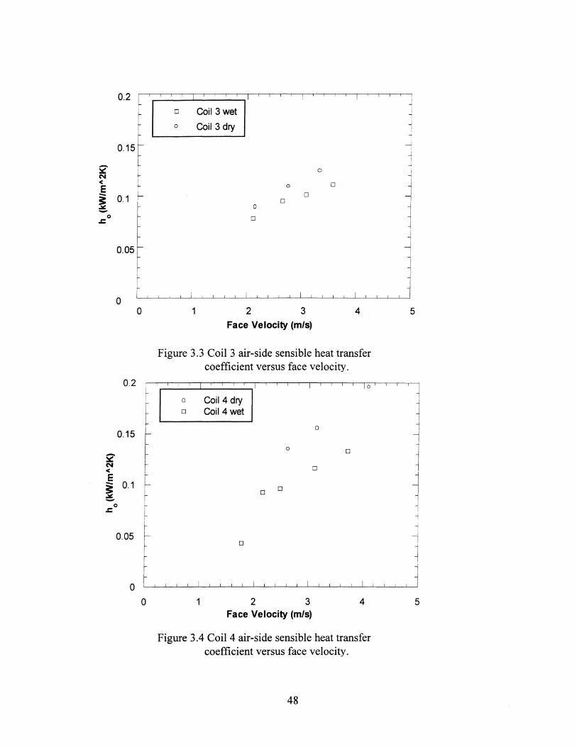
~ N < E -~ -

.J:. 0

~ N <

0.2 L ~

015~ l f-

0.1 r-

0.05

1 i-

0 0

0.2

0.15

E ~ 0.1 ~

o .J:.

0.05

~ ~ I-

1 1 I 1 1 1 1 ,

0 Coil 3 wet

0 Coil 3 dry

0

0 0

0 0

0

0

1 i 1 1 , 1 1 1 1 1 1 1 1 1 I 1

1 2 3 4

Face Velocity (m/s)


1 1 1

I

I ~

J 1

--!

..i

I

~ -j

j ~ ~

1 --<

~ j

1 , 1 I

5

I I I I I i I I i I I I 10 1 1 1 1 J o Coil 4 dry o Coil 4 wet

o

o

o

o o

o

o

~ l ~

I

1 -j

-l I

I ~

~ ~ ~ 1

o L! --'-I -,1'--.11'--.11---1---1.1---1.1 ---1.1 ----'-I ----'---1..1 --'-, ---,-I --'-.1 --'-_''--.1'---11---1.1---1.---1.1 ----'-I ----'-I ----'-, ---1j

o 1 2 3 4 Face Velocity (m/s)


48

5

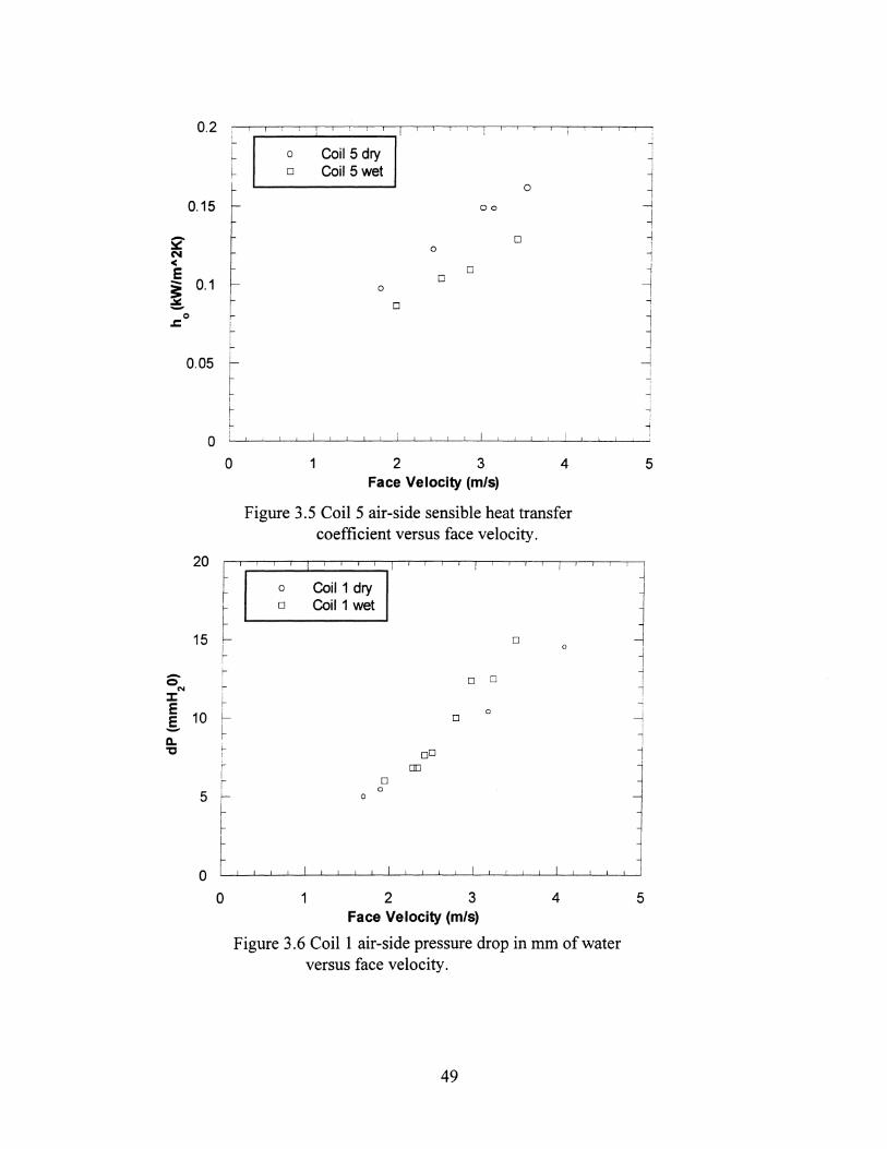
0.2 I i i i i i i I i i i ! i i i

r Coil 5 dry

~ 0

0 Coil 5 wet 0

0.15 - 00

2' 0 0

N < E 0 - 0.1 f-

0

~ 0

0 0 I-.=

t I

0.05 r I

I I-

0 !

i i I i i i i I i i i i I i i i i i i i

0 1 2 3 4 Face Velocity (m/s)


20 i i I i i i i i i

f

i i I I I I I i i I i i

I 0 Coil 1 dry

I 0 Coil 1 wet

15 f- 0

~ 0

Q t- o 0 N I-

::I: I

E ~ I 0

.5. 10 ~ 0

a.. "C ~

00 i

I- m I 0 r 0

5 f- a

~

o o 1 2 3 4

Face Velocity (m/s)

Figure 3.6 Coil 1 air-side pressure drop in mm of water versus face velocity.

49

I

l

1 -I

~ ~ !

-< I

~ -j

I

J ~ I

-j

-I ,

1

5

'] j ~ -1 l ~

i

-1

5

20

~ I I I I I I i ! I

-j

0 Coil 2 dry i

I -j

t 0 Coil 2 wet 1 ~

I ~ 15 --l

i - 0

o 1 0 N

:I: l-E E 10 r- 0 0 -i -

l 0

~ c. 0 0 "C 0

0

0 0 ! 0 5 ~

I- 0 -j ,

I f- 0 1

~ 0 ~ 0 I ,

i -j

0 , i I I i I I i I I I i I I I I I I



20 I I I i I I I I I I I I I I I I I I I

J ~

I 0 Coil 3 dry

I I-

~ 0 Coil 3 wet

~ 15 0

-I 0 i

N I-

j :I: I

0 0 f-E

10 ~ .§. 0

c. r 0 0 "C r

~ 0 -j

:- 0 ~ 5 ~

,

0 1 f0-

r ~

t i

-j

0 I I I I I I I I I I I I I I I I I I I I j

0 1 2 3 4 5

Face Velocity em/s)


50

-0 N

:J: E E -Q. 'tJ

Q N

:J: E .5. Q. 'tJ

20 ,I I I

0 Coil 4 dry 0 Coil 4 wet 0

15 - 0

0

~ 0

~ 10 0

0

l- 0 I

0 r ~ 0

i 0 r-

5 i

CP '-e- o ; 0 ~ 0 L !

0 [

I I I I I I I I I I I I I

0 1 2 3 4 Face Velocity (m/s)


20 I I I I I I I I I I I I I I I I I I I

f I 0 Coil 5 dry

I 0 Coil 5 wet 0

I-15 f- 0

0

~ 0 0

l-

0

i Do 10 f---

I

f 0

0

~ 0

5 0

0

o o 1 2 3 4

Face Velocity (m/s)


51

...,

1 l -i

j I

-: -i l ...i

I

-.j

~ I j 5

I l

~ ~

J I

-1

j

5

0

0 0 - 0.1 ! o cPo 0 t- o 0 c- o

'"" L 0

;- 0 Coil 1 dry j I- 0 Coil 1 wet j i ...

0 0 Coil 1 dry f , f... .., I 0 Coil 1 wet f I I I

I -I

I ,

I 0

~ 0

r 0 0

0 0 0

I DO

0 0 0

0 I I 0 , 0

I 0.01

200 400 600 800 1000 1200 Re

Oh

Figure 3.11 Coil 1 j and f factors versus air-side Reynolds number.

I

I I - I 0

~ 0.1 c-D 0 -'

0 ~ 0 0 ~ 0 0 a l 0

0

0 0 o 0

1 ... 0 0 Coil 2 dry j

0 Coil 2 wet j 0 Coil 2 dry f

I 0 Coil 2 wet f !

I 0

I I- 0 -] I 0

0 00

Cb 0 0 0 0

0.01 200 400 600 800 1000 1200

Re Oh


52

i I

.... I

0.1

~ I .. I

0 ! f-I

~ i

;-

:

0.01

200

I ....

0.1 I-

.. 0

0.01

200

0 Coil 3 j dry 0 Coil3j wet 0 Coil 3 fdry

0 0 0 Coil 3 fwet 0 0

0 0

0 0

0

0 0

0 c 0

0 0

400 600 800 1000 ReOh


I I I 0 Coil 4 dry j 0 Coil 4 wetj 0 Coil 4 dry f

0 0 Coil 4 wet f ° 0 0 0

0° 0 0

° 0 0 0 0 0

o o o o

o o o

400 600 800 1000 ReOh

Figure 3.14 Coil 4 j and ffactors versus air-side Reynolds number.

53

I

J ..J

I

1 "1

] i I

1 I

-I i I I

! -;

I

1200

l

1 1 ~

1200

....

... 0

I

o 0

00 o I 0.1 '-

t o 0

0.01

I

I :-

I

~ I

t I

I , I

200

o

o

o

Coil 5 dry j Coil 5 wetj Coil 5 dry f Coil 5 wet f

o

o

400

o o 0

o o 0 o o o o

600 800 1000 ReOh


350 ~ I' " '" o V,=1.31

300 '--___ ---I.

, , I

o 0 o

00

250 -< 000

: 200 r ,,-o-/a-<> O-o~ ~o~ O-o~ ~o_ ~ 150 ~ i I

l 1

l -j I I

l l I

j 1200

0.03

o 0.025

0.02

0.015

-i :-

100 f 50 ~

t ~

~ ~ v,=l'l ]

0.01

0.005

O~-L~~~~-L~~~~~~~~~~~~~~~ o 3000 o 500 1000 1500

Time (5)

2000 2500

Figure 3.16 Real time condensate retention and humidity ratio for Coil 5 versus time.

54

::I: c 3 ~ = 0

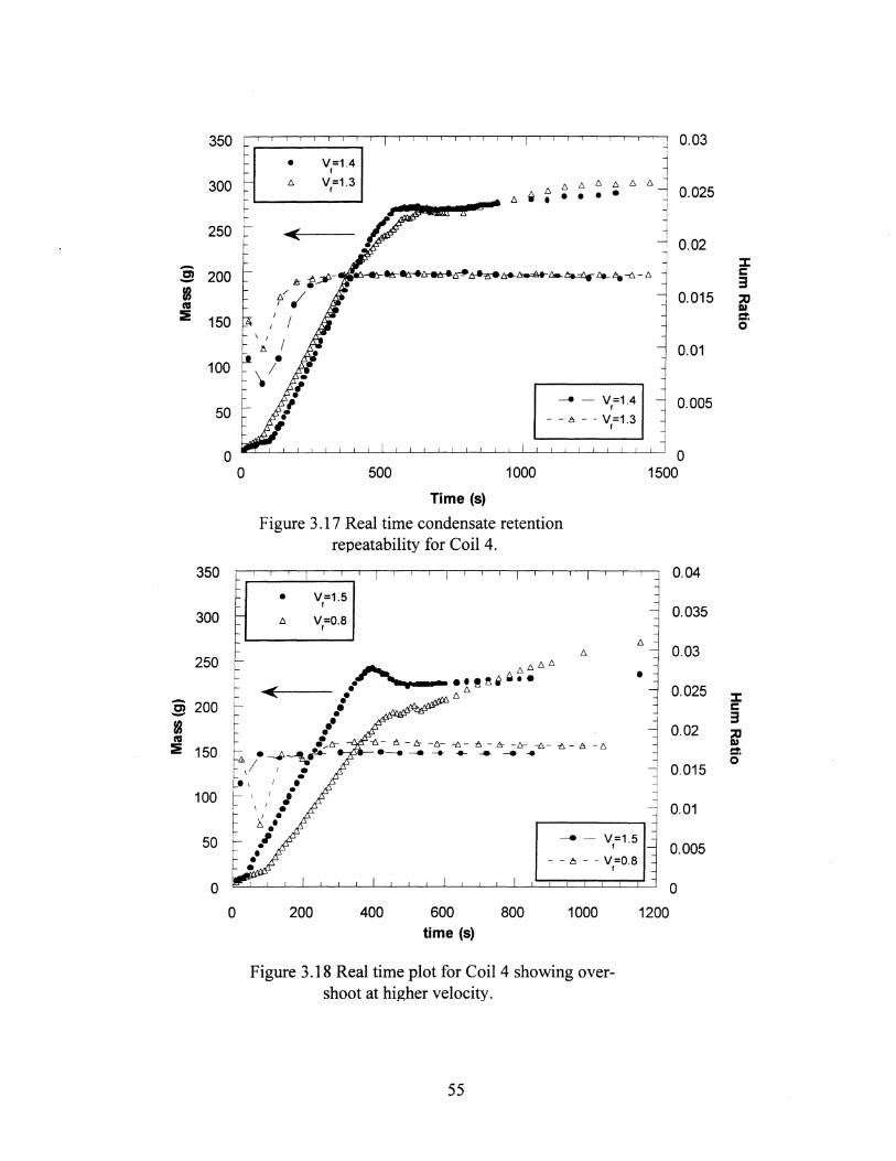
350

300

250

-en 200 -IS co :E 150

100

50

0

350

300

250

- 200 en -IS co :E 150

100

50

o o

i i

~ I ~ !->-f-

0

i

• I j iii I I I I Iii I I f iii Iii

-i 0.03 V=1.4 , V=1.3 , 6~

-1 0.025

j -1

~~~~6*-~;le..~e:...~-6-6 j 0.02

0.015

500 1000

Time (s)

0.01

- - V,=1.4 0.005 - - 6 - - V,=1.3 ~

o 1500

Figure 3.17 Real time condensate retention repeatability for Coil 4.

• V=1.5 , 6 V,=O.8

200

-{;- to -IS -6- -{;- to -IS -/r -{;- -6- 6-6 ._- ....... __ ..

6

•

- - V,=1.5

- - 6 - - V=O.8 ,

i 1

400 600 time (s)

800 1000 1200

0.04

0.035

0.03

0.025

0.02

0.015

0.01

0.005

o

Figure 3.18 Real time plot for Coil 4 showing overshoot at higher velocity.

55

::I: c 3 1I cr. 0

::I: c 3 1I cr. 0

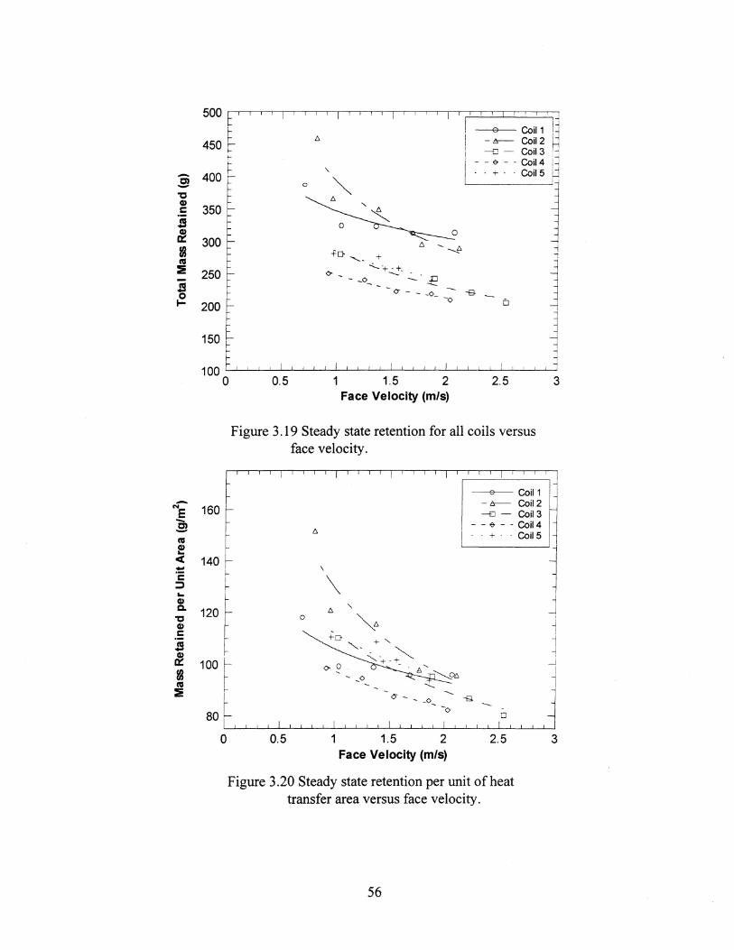
§ "C Q) c S ~ IS CIS

:::lE

-5 ~

-N

E -.9 CIS

~ <C :: c

:::J ... Q) c..

"C Q) C

s ~ IS CIS

:::lE

SOO E i i i I i i I i i i I i i i I i i i r I i i i

i~ f- 0 Coil 1

4S0 ~ /::, -~ Coil 2 I- ---£l - Coil 3

[j ~

- - (> - - Coil 4 i~ 400 ~ "- T-

~i151 0 ~ /::,

3S0

300 /::, ~

---.f1 +0- + "'---

2S0 <>- -,+-+-

----- _0_ -E <Y-_ -0_ --B-

~

200 ~ -0 []

1S0 ~ f--

r-100 t i i i I i i i i I i i i i I i i i i I , i i i I

0 O.S 1.S 2 2.S Face Velocity (m/s)

Figure 3.19 Steady state retention for all coils versus face velocity.

Coil 1 Coil 2

160 r -[] - Coil 3 - - (> - - Coil 4

- + - - Coil5

140 t \

! \ i ~ I "-

120 r /::, 0 ~/::,

+0- + "-

~ ""-- - ~ 100 r <>-9

~-+ .+- , /;:,

~/::, t - _0 "-.

I <Y - ----- _0 --g

80 ti - -0

D

i i i I i i i i I i i i i I i i i i I i i i i I i i i

0 O.S 1 1.S 2 2.S Face Velocity (m/s)

Figure 3.20 Steady state retention per unit of heat transfer area versus face velocity.

56

--i

j ~ ~

-j ]

i -;

3

-i

'~ j 1 1 -1 -i

j -i

I

J j

3

iii 1 Iii ill 1 i i i , i

Run 1 Run 2 Run 3 I :

r

200 ~ o t I Iii Iii iii iii Iii iii iii iii iii I

450

440

430

-420 S IB ~ 410

400

390

380

o 50 100 150 200 250 300 Time (5)

Figure 3.21 Drainage test plot for Coil 3 illustrating the repeatability of the experimental technique.

I I i i I ! i I 16 1 I i I i !

i i I

f 0

0 ° Run 1 >-

Run2 !- 60 0 >- °0 >- 6 Run 3 ~ 60

°

~ 6 0 S 6 C

I 6 (,)6

~ 6 ~go

1:16 00 6 00 0

6 0 666~

0 ° 6 bl

~ 6 g

6 0

~

I

L i i i I i i i I i i i i I i i i i I i i i

0 50 100 150 200 Time (5)

Figure 3.22 Partial plot of the repeatability test results showing the area of maximum error.

57

i I i l l l l

I

] I

-1 -j

-1 i I

350

-, --<

~ ---J

~ j

~ -1 J

-1 -:1 ~

~ J 4

--< -I

i j

250

400 r i I i I i i i i i ! I i i i I l ...,

0 Coil 3 ~ t-

350 c- D Coil 4 l l-i- t:;. Coil 5 r J

~300 t -j

1 - ~ .9250 -1 CIS j f 0

~ 200 -1

0

1 G) 0eo .. r ~=- 0 0 0 0 0 0 0 i ~ 150 ~D.A~ t:;. t:;. t:;. t:;. t:;. I 'L[u~, 0 0 0 0 0

100 ~

~i ~ ~

i I II! I ! ! I 1 i ! J

50 I ! ! i I i i i I I i i

0 50 100 150 200 250 300 350

Time (s)

Figure 3.23 Dynamic test results for the fast draining coils.

450 I I I I I I

0 Coil 2 400 - -

0 Coil 6 350 - t:;. Coil 7 --N

< ~ E 300 f-Ooo --CD Cb~COCOooo -CIS f 250 - 0

0 -0 « ~6t:;.~

0 0 ... 0 0 j G) Co 200 -1 IS

~Mt:;. t:;.

-j

6 -I

CIS t:;.

:E 150 0 t:;. t:;.

~ t:;.

100 0 0 0 0 0 0 0

50 0 50 100 150 200 250 300 350

Time (s)

Figure 3.24 Dynamic test results for the sustained draining coils.

58

250

_ 200 N < E S co 150 e

<C ... G) Q.

II! 100 co :!

8 Coil 3

-El-- Coil 4

--<> - Coil 5

----6---- Coil 6

,

"1 ,

-,

- - + - - Coil 7 ~

~~~-~-~~~~-----~--~~~~ l 6- __ -+------ ]

- - - -Lot - _ _ _ _ - + - - • - _ _ _ _ ~ 50 -'-'------6 +- - - •• - - - oj----j

~ • -. - -- - - -. - - - -Lot - - - - •• - • -. - _. ____ " -6 i

f-r ~ o L[ ---"--'-' ---L' ---"--'-' ----'-' ---1'--'-' ----'-' ---11--,-, ----'-' ---1'--'-' ----,-, ---'---'-'----'-' ---,,--,-1----,-, ---"--'-'----'-' ---"---'-'----'-' -'---'-'--"

500

450

400

350

c; - 300 II! co :!

250

200

150

100

o 5000 Time (s)

Figure 3.25 Extended time drainage test results.

l i i i I i i i i i i i i i I i i i I i i i

'1 I

• Vertical 6 Tilted

1 r· F···-..-..... • 1 • • • • ~6 -i

E- 6l1l1l1

-j ~ -i J

~ ~6 6 6 6 6 ~ r- 6 6 6 -l I

~ r-

~ j r-

~

[, i i i I i i i i I i i i I i i i i I i i i i I i i i i I i i I J

0 50 100 150 200 250 300 Time (s)

Figure 3.26 Comparison plot between a vertical coil and a coil tilted 10°.

59

350

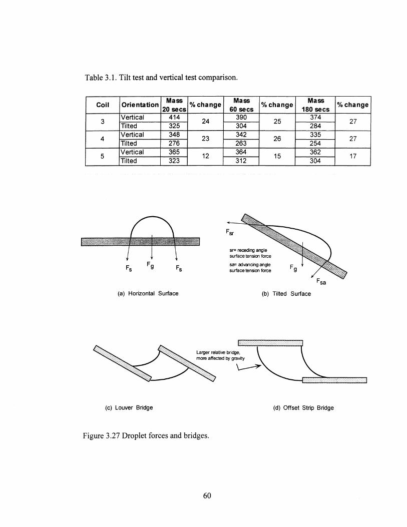
Table 3.1. Tilt test and vertical test comparison.

Coil Orientation Mass

20 secs

3 Vertical 414 Tilted 325



(a) Horizontal Surface

(c) Louver Bridge

% change Mass

% change Mass

60 secs 180 secs

24

23

12

390 304 342 263 364 312

Fsr

sr= receding angle surface tensioo force

sa= advancing ange surface tensioo force

25 374 284

26 335 254

15 362 304

(b) Tilted Surface

Larger relatil.e bridge, more affected i:1{ gravity

(d) Offset Strip Bridge

Figure 3.27 Droplet forces and bridges.

60

% change

27

27

17

Chapter 4 Conclusions and Recommendations

Heat transfer, pressure drop, and retention data have been collected and presented

for five automotive evaporators. The thermal performance tests were conducted under dry

and wet conditions and both steady-state and transient retention data were recorded.

Additionally, a dynamic drainage test was developed and a variety of coils tested. This

chapter contains general conclusions about the effects of condensate on the overall

performance of an automotive air-conditioning system, and a recommendation for the

focus of future work in this area.

4.1 Conclusions

4.1.1 Thermal-Hydraulic Performance

The heat transfer coefficient decreased and the pressure drop increased for all

coils tested. Condensate retention causes the decrease in heat transfer coefficient by

forming bridges in the inter-louver space and redirecting the flow from the desired

louver-directed flow to duct-directed flow. Additionally, condensate may also form

bridges between fins effectively creating a dead region on the fin. Larger louver pitches

helped prevent louver bridging, but decreased absolute performance of the coil due to

reduced boundary layer restarting (and resulting thicker boundary layers).

The pressure drop increases under wet conditions even though the flow is

redirected into duct flow and that would seem to decrease pressure drop. The presence of

condensate on the fin surface decreases the effective minimum flow area and causes

increased pressure drop. This effect will be even greater with the presence of fin bridges.

Coil 4 was shown to have only a slight increase in pressure drop from dry to wet

conditions, and a corresponding lower quantity of retained condensate.

61

4.1.2 Condensate Retention

A highly repeatable method of measuring condensate load-up on evaporators was

developed. The quantity of retained condensate reached a steady value in 15-25 minutes

depending on operating conditions. The greater the water mass-flux the shorter the time

to reach steady-state, as expected. At some specific air-flow rates, an initial 10%

overshoot in condensate retention was observed. This effect may be important in

determining the drainage characteristics of a coil. It was hypothesized the relative

quantity of condensate draining through different modes causes the overshoot, though

further experiments are required. Extended test runs were done to investigate the

possibility of oscillations in retention caused by shedding mechanisms that may impact

the performance characteristics and data interpretation methods. However, the quantity of

condensate remained within 1.5% over a 45 minute test, once a steady value was attained.

Steady-state retention results showed a large influence of frontal velocity on the

quantity of retained condensate for all the tested coils. The impact of the airflow shear

forces varied with geometry over the tested range of face velocities. At the highest

velocities the quantity of retained condensate for similar geometries (same heat transfer

area, different louver designs) showed a slight tendency to converge, indicating that shear

forces start to dominate gravity forces and geometrical influences on retention. A large

turnaround section, similar to the centerline divide investigated by Osada and coworkers

(1999), resulted in lower condensate retention in Coil 4 compared to Coil 5, though the

impact of the higher louver angle is unclear. However, heat transfer was observed to

decrease by a greater amount in Coil 4 under wet conditions, likely due to a lower

absolute number of louvers without condensate bridging.

62


A dynamic drainage test apparatus was built to test the drainage of a variety of

coils. Initial drainage response (in a 300 second interval), 10ng-teInl drainage, and

orientation effects were investigated. Two distinct drainage patterns were observed; fast

draining coils that reached a steady-state value within about 120 seconds, and sustained

drainage coils that continued to substantially drain water for up to four hours. The long

teInl results, and the results of the tests with the coil face tilted 100 from vertical show the

influence of louver bridging on drainage. When a louver bridge exists, gravitational

forces are not sufficient to remove the bridge unless the bridge is very large, such as one

that may exist between offset strips. Thus, in 10ng-teInl testing, louvered fins drain much

slower than offset strip fins. This drainage behavior is potentially important to biological

growth on the fin surface.

The drainage tests also qualitatively predicted the condensate retention in the

wind tunnel for Coils 2 through 5; that is, the rank-order for condensate retention in

wind-tunnel testing was congruent with the drainage test results. The drainage test over

predicted the absolute quantity of retention, but with the large influence of shear forces

on retention this result would be expected. The drainage test reflects retention at the zero

velocity operating condition. Furthermore, the test procedure developed is more accurate

than traditional 'dip-test' methods, because the relative rates of drainage are important.

4.2 Design Guidelines

In order to compare two fin designs and one design declared 'better', it is

necessary to define the objective function as it relates to system perfomlance. The

optimized design attributes can be any combination of the following parameters.

63

1) Higher heat transfer coefficient, under either dry, wet, or wet compared to dry.

2) Lower pressure drop across the coil, again under either dry, wet, or wet

compared to dry.

3) Lower quantity of condensate retention, under operation or post-operation.

A higher heat transfer coefficient is obviously desirable to either increase the heat duty of

a heat exchanger or alternatively and perhaps more importantly, decrease the size of the

coil while maintaining the same capacity. A lower pressure drop is beneficial because of

pumping power and noise. Overall system efficiency will be improved if less pumping

power (the blower fan in automotive applications) is required. Increased blower speed

also generally causes increased noise levels. As discussed in the introduction, water

remaining on the air-side surface of an evaporator coil after system shutdown is a prime

environment for biological activity, and the result is a degradation of air quality through

odor and thermal performance through fouling. In summary, care must be taken when

rating heat exchangers and developing design guidelines, as it is critical to define the

proper objective function based on the focus of the optimization. From the results of this

study, the following are recommended design guidelines for improved fin design:

• Keep louver angle at or below 36°. The comparative results of Coils 4 and 5

showed only a slight increase in heat transfer coefficient from using a 42°

louver and large increase in core pressure drop.

• Increase the effect of the turnaround section on condensate drainage by

increasing the length or openness of the turnaround section, effectively

dividing the fin. One interesting possibility is to actually remove part of the

heat transfer surface in the center. This may allow a smaller 'drainage' section

64

to obtain the same benefits, thus leaving more area for the high heat transfer

louvers.

• Offset-strip fins appear to drain condensate better than louver fins over the

long-term, such as after system shutdown (a tentative conclusion based on

limited test results), and as discussed should form less condensate bridges.

Thermal-hydraulic performance data for offset strip arrays would be required

to further quantify potential benefits of that design.

4.3 Recommendations for Future Studies

There are several areas where additional research can either enhance the ideas

generated in this study, further the condensate retention modeling efforts, or refine the

design guidelines for developing improved fins. Three specific research directions are

discussed in this section.

Drainage and sweeping effects for automotive evaporators are substantially

different from plain-fin coils, there are important interactions between fins and fins and

fins and tubes in the automotive evaporator. As a result, it is expected the wet

performance of the fins vary will vertically in the fin column due to condensate

distribution. The variance in heat transfer coefficient from top to bottom in the fin array

would be important to determine both the impact of condensate on performance and

refine the retention model by indirectly predicting how much louver and fin bridging

exists. McLaughlin and Webb (2000) suggested that lower header design is key to

determining how much condensate will 'back-up' vertically in a coil, and vertically

resolved performance data would also develop this idea. A heat exchanger could be

partitioned into thirds or fourths vertically by embedding thermocouples in the tube at

65

specific points depending on circuiting, and matching the downstream air temperature

thennocouples to the tube locations.

Related to vertical partitioning, is more sophisticated single fin column testing

with optical access. One of the keys to condensate modeling is predicting the droplet

distribution on the surface, and the highly compact geometry of automotive evaporators

make it virtually impossible to observe the fins during operation. Previous efforts at

single column testing (Osada et aI., 1999, and McLaughlin and Webb, 2000) used only

single-sided cooling of the fin, which could affect the distribution on the fin, and

definitely affects the distribution on what would be the outer tube surface. The tube-side

geometry also needs to be closely matched; however, this will be difficult to accomplish

while maintaining optical access, as will cooling both sides of the fin. However, one

solution may be to treat the inside of the glass to make it hydrophilic, and then make

observations through the water film. This would at least allow a better approximation of

drainage routes. Cooling the tube surface would be easier, as dry, refrigerated air could

be blown across the outer surface. Results of single column tests would yield important

observations required to model droplet, and more importantly, bridge distributions along

the fin depth and height.

The final recommended research focus is in asymmetric fin design. All the fins

tested in this study (and in the open literature), are symmetric along the fin depth

centerline. The large influence of shear forces on condensate retention necessarily means

there exists a condensate distribution along the fin depth. Fin designs that have good heat

transfer characteristics do not necessarily manage condensate effectively, and by

designing the fin to promote high heat transfer in the front of the fin and better

condensate drainage in the back, overall perfonnance can be increased. The larger gaps

66

within an offset strip array may have a tendency to form less condensate bridges.

McLaughlin and Webb (2000) noted the louver cut end provides an area where a

condensate meniscus can easily grow into a louver bridge. A true offset strip would have

no narrowing at the cut end. Offset strips though, do not have the heat transfer

performance for the same fin depth as louvers. So a potentially superior fin design is to

use small pitch high angle louvers for the highest possible heat transfer in the front of the

array and offset strips or larger pitched louvers in the rear of the fin to decrease bridging

and promote drainage. The actual configuration of the design would be a primary

objective. Initial experiments on scale-up models would be an efficient technique to

determine a starting point for an optimal design. Single fin column testing would also be

useful, and a modular type test specimen could be built with partial fins that are different

types of louvers and offset strips could be built and different configurations could be

easily tested.

67

Appendix A Data Reduction

This appendix describes the data reduction techniques used for this study. Many

of the parameters are straightforward calculations. Further discussion of the calculations

is presented as needed. The output file from the data acquisition system and the manually

recorded data described in Chapter 2 are used as the input variables for the main data

reduction routine maintained on a commercial equation solver, Engineering Equation

Solver (EES). The advantages of using EES are the thermophysical property functions for

moist air are built in and a parametric table can be used to manage multiple test runs. The

EES code used for the data reduction is shown in Tables A.I and A.2

A.1 Mass Fluxes

The coolant-side mass flow rate was calculated from the density and volumetric

flow rate; measured with a flow meter that provided a 5-volt dc pulse with 1.849xI06

pulses per cubic meter of liquid. Equation A.I was used to calculate the coolant mass

flow rate where Re is the number of pulses per second. The outlet coolant temperature

was used to calculate the coolant density since the meter was located on the return line.

. R ( I ) me = ePe I.849xI06

(A.I)

The air-side mass flow rate was calculated from the frontal velocity, flow area,

and density. The velocity of the air at the heat exchanger face was measured using a

constant temperature thermal anemometer. The anemometer was calibrated by the

manufacturer at standard temperature and pressure so the measured velocity needed to be

corrected based on the temperature and pressure at the heat exchanger face. The actual

velocity was calculated using Equation A.2.

68

v = V (273 + Tfr J(101.325J fr,c fr 294.1 Patm

(A.2)

The atmospheric pressure is measured with a NOV A laboratory barometer and the air

temperature is from the upstream thermocouples. All other air properties were computed

using thermophysical property functions that were built into EES.

A.2 Heat Transfer Rates

Equations A.3 through A.5 were used to calculate the heat transfer rates.

Calculations were based on measurements made at the test section inlet and outlet. The

data used for this study required that air-side and coolant-side heat transfer rates were

within 10% including the bias error discussed in Appendix B.

(A.3)

qrol = rh air (hin,air - houl,air) (A.4)

(A.5)

A.3 Fin Efficiency

The fin geometry in the tested automotive evaporator coils can be modeled for fin

efficiency calculations as a straight fin with an adiabatic tip. Furthermore, the adiabat for

each fin is taken as the centerline due to circuiting and coolant flow rates. Most of the

heat exchangers tested use a parallel flow manifold with three coolant passes so each side

of the fin is at the same temperature with the exception of the two fins that are along the

turnarounds. Additionally, the coolant flow rate is such that the temperature change is

between 1.5 and 5.0 degrees Celsius, so any deviation of the adiabat from the centerline

for any fin will be much smaller than the fin width.

69

Fin efficiency for the dry condition tests was computed using a standard equation

commonly found in heat transfer texts (for example Incoprera and Dewitt, 1990). The

expression for a straight fin with adiabatic tip is,

(A. 6)

where,

(A. 7)

For fins where the fin width is much greater than fin thickness ma reduces to

(A.8)

For calculating the fin efficiency under condensing conditions when the fin

surface is full wetted, the method presented by Wu and Bong (1994) is used. They

consider the driving forces for heat and mass transfer separately. Wu and Bong assumed

a linear relationship between OJ s' the humidity ratio of the saturated air at the wet surface,

and 1'., the surface temperature. This assumption allowed them to analytically solve the

governing fin surface temperature differential equation when the Colburn-Chilton heat

and mass analogy holds. Namely, the heat transfer coefficient and the mass transfer

coefficient are related by

h 2/ _0 = CpLe/3 hm

(A.9)

With the fin surface temperature distribution known expressions for the heat transfer

from the fin and the maximum heat transfer (occurring if the entire fin was at the fin base

temperature) are derived.

70

(A.lO)

(A. 1 1 )

Where m is related to ma in the dry fin equation by,

(A.12)

(A.13)

and b is the average slope of the saturation line on the psychometric chart from

0) -0) b = s,t s,b

1; -Tb (A. 14)

The fin efficiency is defined as the ratio of heat transfer to maximum possible heat

transfer. Hence,

tanh(mL) 17f =

mL (A.15)

which is same as the expression for fin efficiency in the dry case with ma modified by Eq

A.12. The fully wet fin efficiency of Wu and Bong is relatively independent of the

humidity ratio of the incoming air,

With the fin efficiency known, the overall surface effectiveness for both wet and

dry conditions can be calculated from,

Af n =1--(1-n ) 'ft A 'If

I

(A. 16)

71

A.4 Heat Transfer Coefficients

A modified Wilson-plot methodology was used to calculate the air-side heat

transfer coefficient. The technique used was an adaptation of the ideas discussed by

Briggs and Young (1969), and presented by Rohnsenow et al. (1985). Wilson (1915)

devised a technique whereby individual thermal resistances could be extracted from the

overall system thermal resistance. The general thermal circuit for the studied heat

exchangers neglecting air-side and tube-side fouling and no tube-side enhancements is:

I I I I I = = = +--+R UA (UA)c (UA)o (17hA)o (hA)c W

(A17)

The basic idea behind building a data set for the Wilson-plot method is to hold one side

of the heat exchanger (the air, or hot side in this study) constant and systematically vary

the flow on the other side. Solving Equation A.I7 for _1_ and grouping terms yields Uc

Equation A18.

(A18)

For turbulent flow through constant cross-sectional ducts, the Nusselt number correlation

has the form of

Nu - C ReO.8 Pr°.4 - ° and an equivalent form of Equation AI8 is

(AI9)

(A20)

72

A plot of _1_ versus ~o 8 with the air-side temperature and mass flux held constant and U v· c

Equation A.19 being valid is linear and has the form of,

y = mx+b (A.20a)

where,

(A.20b)

The slope and intercept of the resulting data set are calculated by a least squares

fit to the data points. Equation A.18 can be solved for 1]ho directly or iteratively for ho

with a fin efficiency equation and j factors can be computed.

Briggs and Young modified the Wilson-plot routine by incorporating the real

possibility that the fluid temperature on either side of the heat exchanger could vary from

test run to test run. Instead of plotting a velocity function they used the tube-side Nusselt

number directly in the form of

Nu, ~ C, Re" prO'(;: J (A.2l)

and proceeded in a similar manner. A linear regression analysis is carried out to

determine the appropriate Reynolds number exponent that minimizes the least squares fit

to the data points.

For this study, further modification of the Briggs and Young technique is used to

construct the Wilson-plot. The tube-side Nusselt number is calculated using the

Gnielinski correlation for transitional flow in tubes:

Nu = (f 18)(ReD -1000)Pr D 1+12.7(fI8)1/2(Pr2/3 -l)

(A.22)

73

where,

(A.23)

The Reynolds number is based on hydraulic diameter, DH = 4Ac . The Wilson-plot was p

constructed by plotting _1_ versus _1_. Thus the linear relationship is, VA NU D

(A.24)

Where the first term on the right hand side is dependent on tube-side Reynolds number

and the second group is independent and held constant by maintaining the air-side

conditions. Furthermore, the wall resistance for the range of Reynolds numbers in this

study accounted for less than 5% of the total resistance and was neglected. The intercept

of the least squares fit line to a single set of Wilson-plot data is the air-side resistance,

(A.25)

This Wilson-plot technique has effectively allowed the tube-side resistance to be forced

to zero by extrapolating to an infinite tube-side Nusselt number. Equation A.25 and the

fin efficiency equations are then solved iteratively to obtain the air-side heat transfer

coeffi ci ent.

The methodology for building a complete set of data is described next. Since the

focus of this study is air-side heat transfer an effort was made to maximize the amount of

air-side data while maintaining the lowest uncertainty. The slope of the Wilson-plot is

independent of the air-side velocity, so the adopted technique was to collect a baseline

data set at an air-side Reynolds number at approximately the middle of the range of

74

interest (-700 based on hydraulic diameter). This baseline data set consisted of Wilson

plot points generated from tube-side Reynolds numbers from approximately 4,000 to

9,000. Subsequent data sets were recorded for other air-side Reynolds numbers (from

-300-1100) at only three or four tube-side flow rates where the Reynolds number varied

between 5,000 and 8,000. The slope of the linear fit to the baseline data set was induced

on all other data sets and the intercept was calculated from a modified, least squares fit.

This technique was really beneficial in condensing experimental test runs because of the

difficulty in maintaining constant air-side conditions for the extended duration required to

record data for the different tube-side Reynolds numbers. An example modified Wilson

plot is shown in Figure A.I.

75

1 I

1 ~

6 I-

--<

I-

~

L

:t I!I A

~ Z!l Z!l

j II

~ e e

• J

.. • •

4

r • • • :.; :.;

~

~ § )( x

9 !iii !iii

"/

3 >-

f3 !iii

i

-~ >-

...

f:

12 t - • Baseline 8 -Re 1

Re2 - ~~ Re3 - !!'! Re4 0

"1

0 0.005 0.01

0.015 0.02 1/Nuo

Figure A.I Example of MOdified Wilson-plot.

76

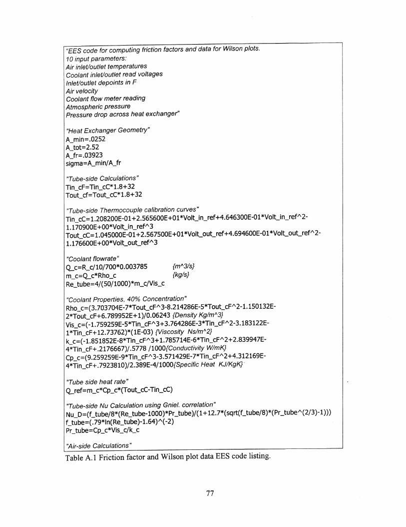
"EES code for computing friction factors and data for Wilson plots. 10 input parameters: Air inlet/outlet temperatures Coolant inlet/outlet read voltages Inlet/outlet depoints in F Air velocity Coolant flow meter reading Atmospheric pressure Pressure drop across heat exchanger"

"Heat Exchanger Geometry" A_min=.0252 A_tot = 2. 52 A_fr= .03923 sigma=A_min/ A_fr

"Tube-side Calculations" Tin_cF= Tin_cC*1.8+ 32 TouCcf=TouCcC*1.8+32

"Tube-side Thermocouple calibration curves" Tin_cC= 1.208200E-Ol +2.565600E+Ol *VoICin_ref+4.646300E-Ol *Volt_in_ref/\ 2-1. 170900E+00*VoIUn_ref/\3 Tout_cC= 1.045000E-0 1 + 2.567500E +0 1 *Volt_out_ref+4.694600E-Ol *Volt_out_ref/\ 2-1. 176600E+00*Volt_outJef/\3

"Coolant flowrate" Q...c=R_c/l0/700*0.003785 m_c= Q...c* Rho_c Re_tube=4/(50/1000)*m_c/Vis_c

{mIl3ls} {kg/s}

"Coolant Properties, 40% Concentration" Rho_c=(3. 703704E-7*Tout_cF/\ 3-8.214286E-5*Tout_cF/\ 2-1.150132E-2*Tout_cF+6.789952E+l)/0.06243 {Density Kg/mIl3} Vis_c=(-1.759259E-5*Tin_cF/\3+3.764286E-3*Tin_cF/\2-3.183122E-1 *Tin_cF+ 12.73762)*(lE-03) {Viscosity Ns/mIl2} k_c=(-1.851852E-8*Tin3 F/\3+1.785714E-6*Tin_cF/\2+2.839947E-4*Tin_cF+.2176667)/.5778/1000{Conductivity W/mK} Cp_c=(9.259259E-9*Tin_cF/\3-3.571429E-7*Tin_cF/\2+4.312169E-4*Tin_cF+.7923810)/2.389E-4/1000{Specific Heat KJ/KgK}·

''Tube side heat rate" Q...ref=m_c*Cp_c*(TouccC-Tin_cC)

''Tube-side Nu Calculation using Gniel. correlation" Nu_D=(Ctube/8*(Re_tube-l000)*Pr_tube)/(1+12.7*(sqrt(Ctube/8)*(Pr_tube/\(2/3)-1») Ctube=(. 79*ln(Re_tube)-1.64)/\( -2) Pr _tu be = Cp_c*Vis_c/k_c

"Air-side Calculations"

Table A.I Friction factor and Wilson plot data EES code listing.

77

Tdp_inC=(Tdp_inF-32)/1.8 (degrees F to degrees C) Tdp_outC=(Tdp_outF-32)/1.8 (degrees F to degrees C) Tdp_inC=DewPoint(AirH20,T=Tin_air,P=P _atm,w=wl) {determine absolute humidity} Tdp_outC=DewPoint(AirH20,T = Tout_air,P=P _atm,w=w2) {determine absolute humidity} P _atm=(P _hg)*convert(inHg,kPa) {Pressure conversion} RH_in=ReIHum(AirH20,T=Tin_air,P=P _atm,w=wl) {Relative Humidity} RH_out=ReIHum(AirH20,T=Tout_air,P=P _atm,w=w2) {Relative Humidity} T _mair=(Tin_air+ Tout_air)/2 w_mair=(wl +w2)/2 Rho_airl =Density(AirH20,T = Tin_air,P=P _atm,w=wl) Rho_air2=Density(AirH20,T=TouCair,P=P _atm,w=w2) Rho_air=Density(AirH20,T= T _mair,P=P _atm,w=w_mair) Vis_air=Viscosity(AirH20,T = T _mair,P=P _atm,w=w_mair) k_air=Conductivity(AirH20,T=T_mair,P=P _atm,w=w_mair) Cpin3ir=SpecHeat(AirH20, T = Tin_air,P=P _atm,R=RH_in) Cpout_air=SpecHeat(AirH20,T=Tout_air,P=P _atm, w=w2) Cp_mair=(Cpin_air+Cpout_air)/2 hin_air=Enthalpy(AirH20,T=Tin_air,P=P _atm,w=wl) hout_air=Enthalpy(AirH20,T = Tout_air,P=P _atm,w=w2) h_mair=(hin_air+hout_air)/2

"Air flowrate" m_dot_air=VoLair*Rho_air {Kg/s}

{Kg/m A3} {Kg/m A3} {Kg/m A3} {Nslm A2} {W/mK} {KJ/KgK} {KJ/KgK} {KJ/KgK} {KJ/Kg} {KJ/Kg} {KJ/Kg}

VoLair=VeLair*Flow_area*(273+ Tin_air)/294.1 *101.4/P _atm "Velocity probe correction" Flow_area=8*.0254*12*.0254 {Wind Tunnel geometry}

V _max=V _air*(A_fr/ A_min) G3ir=V _max*Rho_air V _air=VoLair/ A_fr Pr _a=Cp_mair*Vis_air/k_air* 1000 Re3ir=G_air*2.30/1000/Vis_air "2.30=hydraulic diameter"

"Heat Rates" CLsens=m_docair*Cp_mair*(Tin_air-Tout_air) q_tot=m_dot_air*(hin_air-hout_air) q_ave=( q_ref+q_tot)/2 CLerr=( q_ref-q_ave )/CLave LMTD=(Large-Small)/ln(Large/Small) Large= Tin_air-Tout_cC Small=Tout_air-Tin_cC

"Wilson Plot Data" Wilsy=(LMTD/q_sens) Wilsx=l/Nu_D

"ffactor" Cair=2*dp*Rho_air/G_air" 2*A_min/ A_tot-( l-sigma" 2)*(Rho_airl/Rho_air2-1 )*(A_min/ A_tot)*(Rho_air/Rho_airl) dp-deltaP*convert(inH20,pa)

Table A.I (cont.) Friction factor and Wilson plot data EES code listing.

78

"EES code for computing j factors 11 input parameters: Atmospheric pressure Inlet/outlet coolant temperatures air mass flux Wilson plot intercept air Prandtl number air specific heat air density air conductivity inlet/outlet humidity ratios"

st=h/(G*Cp_a) j=st*PrA(2/3)

eta_fin=tanh(m*L)/(m*L) m_O=sqrt(2*h/(k*thickness» m=m_O*sqrt(l +b*xi) thickness= .004*convert(in,m) k=.154 {kWlm K} L=.15625*convert(in,m) eta_o=l-A_fin/A_t*(l-eta_fin) A_t=2.542 2.296=A_fin

\\ Wu and Bong" (theta+theta_p)/(theta_b+theta_p)=cosh(M*(L-finwidth»/cosh(m*L){fin temp. distribution)

finwidth=.15625*convert(in,m) theta=T _a-T_t theta_b= T _a-T_b theta_p=xi*C_O/(l +b*xi)

xi=h_fg/(Cp_a*LeA(2/3» b=(w_s_t-w_s_b)/(T _t-T _b) a=w_s_b-(w_s_t-w_s_b )/(T _t-T _b)*T_b C_O=w_a-a-b*T 3 w_s_t=humrat(AirH20,T=T_t,P=P _atm,D=T_t) {Hum ratio at fin tip} w_s_b=humrat(AirH20,T=T_b,P=P _atm,D=T_b) {Hum ratio at fin base}

Le=k_a/(rho_a*Cp_a*D_AB)/1000 D_AB=( .00143*T _aA 1. 75)/(P _atm*M_ABA .5*(Sigma_nu_AA( 1/3)+Sigma_nu_BA(1/3»)A 2)

Sigma_nu_A= 19.7 Sigma_nu_B= 13.1

M_AB=2*( l/M_A+ l/M_B)A( -1) M_A=MOLARMASS(Air) M B=MOLARMASS(Steam)

Table A.2 j factor EES code listing.

79

rho3=density(airH20,P=P _atm,T=T_a,W=w_a) w3=(wl +w2)j2 h_fg=h3-h2 h2=ENTHALPY(Steam,x=O,P=Pl) h3=ENTHALPY(Steam,x= 1,P=Pl) Pl=PRESSURE(Steam,T=T_a,x=O) 2*T b=Tin C c+ Tout C c

Table A.2 (cont.) j factor EES code listing.

80

Appendix B Uncertainty Analysis

Uncertainties in the experimentally measured and reduced data are presented in

this appendix. The errors in the measured parameters are discussed and propagated to

estimate the uncertainties in the calculated parameters. Most of the uncertainty

calculations are straightforward, but several warrant discussion and clarification.

B.l Uncertainty in Measured Parameters

The errors associated with the various experimental measurements are shown in

Table B.1. The dewpoint of the air was measured by chilled mirror hygrometers at the

inlet and outlet and had a measurement uncertainty of ±0.2°c. Coolant flow rate was

measured using an oscillating disc type flow meter with a measurement uncertainty of

±1.0%. Air-flow velocities were measured using a constant temperature thermal

anemometer with a calibrated uncertainty of ±2.0% of the measured reading. Finally, an

electric manometer with an uncertainty of ±O.l24 Pa was used to measure the air-side

pressure drop across the heat exchanger. Type-T thermocouples were used to measure the

air temperature and the coolant temperature. Each thermocouple was individually

referenced to a thermocouple located in an ice bath and calibrated to a NIST traceable

mercury-in-glass thermometer. Calibration data were fit with fourth order polynomials

for each thermocouple. The uncertainties associated with the thermocouples were ±0.2°c.

A precision electronic balance was used to measure condensate quantities and had an

uncertainty of ±0.1 grams, which is less than 0.05% over the entire range of

measurements and will normally be neglected.

81

B.2 Uncertainty in Calculated Values

The uncertainties in calculated experimental values were detennined usmg

techniques by Kline and McClintock (1953). The propagation of error through the data

reduction equations introduces an uncertainty in calculated parameters. Equation B.l was

used to detennine the uncertainties in the calculated values.

Wy = :t BY W [( J 2]~ m=l BXm m

(B.l)

Where Wm = uncertainty of variable m=I,2,3, ... ,n

W y = propagating uncertainty in result

BY = partial derivative of result with respect to variable m. BXm

When Y is simply related to Xm by the following fonn,

(B.2)

then Equation B.l may be rewritten as,

Wy -:t Xm [ ( w J2]~ Y m=l Xm

(B.3)

B.2.1 Tube-side

A. Heat Transfer Rate

The uncertainty in coolant heat transfer rate is calculated using Equation B.4,

where the first three tenns on the right hand side is uncertainty from the mass flow rate.

As published by the manufacturer, the volumetric mass flow rate meter has an uncertainty

of 1.0%. Using a conservative 2.0% uncertainty in the ethylene glycol mixture properties

82

the uncertainty in tube-side heat transfer rate is estimated to be 10%. However, in the

beginning of this study, it was determined a bias error of approximately 5% existed

where the computed heat transfer rate on the tube-side was lower than the computed heat

transfer rate on the air-side. Different sources of error on both sides of the heat exchanger

were investigated and it was concluded the immersion thermocouples on the tube-side

were the cause. The coolant flow-rate was required to be relatively large to maintain

turbulent flow through the heat exchangers and this caused tube-side temperature

differences ofless than 2.0°C giving an uncertainty of 10% from the thermocouples. The

actual bias error is probably the result of errors in the calibration that are compounded by

the high uncertainty in temperature reading. The errors in the average heat transfer rate

were very consistent and varied less than 4% from the 5% bias, giving an overall

uncertainty within 10%.

Wqc = [(WP<.OUI )2 +(WRc)2 + (l.O%Y +(Wcp)2 +(WtlT)2]h qc Pc.out Rc Cp!1T

(B.4)

B.2.2 Air-side

A. Vrnax

Equation B.5 was used to determine the propagated uncertainty for V max. The

frontal velocity was measured directly using a constant temperature thermal anemometer

with an uncertainty of 2.0% in the measured reading. Heat exchanger dimensions were

measured using a caliper with an uncertainty of 0.025 mm., and the uncertainty for each

parameter is based on number of measurements required. Amin has an additional source of

83

error due to orientation when the coil is placed in the wind tunnel and is approximately

4%. The uncertainty in Vmax was 6% with an uncertainty in Afr of2.0%.

WVmax = [( WV~ir)2 + (WAfr J2 + (W ~io)2 + (Wp~" )2]Yz V max Valr A fr Amm PaIr

(B.5)

B. Reynolds Number

The uncertainty in air-side Reynolds number based on hydraulic diameter is

calculated using Equation B.6. The uncertainty in hydraulic diameter is approximately

1.5%, and the uncertainty in air mass flux is the same as for V max, 6%. Therefore, the

uncertainty in Reynolds number is approximately 6.5%.

~ ~ ~ ~ w. [(W)2 (W )2 (W )2]Yz ReDh = Gair + Dh + Pair

(B.6)

C. Friction Factor

The uncertainty in air-side friction factor is determined by Equation B. 7. With an

uncertainty in A tot of 4.5% the uncertainty in air-side friction factor is calculated to be

12%.

+(WA~in)2 +(WAIOI)2 Amm Atot

(B.7)

84

D. Heat Transfer Coefficient

The difficult factor in determining the uncertainty in heat transfer coefficient is

estimating the error in the Wilson plot intercept. As detailed in Appendix A, the Wilson

plot is constructed by plotting llUA versus 1INutube and fitting a least squares line to the

data for each air-side condition. The variance in the intercept for a single line can be

estimated using an equation from Beers (1957),

(B.8)

Where k is the number of samples and the first term is the estimated variance in y. The

95% interval can now be used to estimate the uncertainty in the y-intercept of a single

Wilson plot line. Several values were computed and the maximum uncertainty for a data

set was 8%. It should be noted that additional statistical analysis would be required to

estimate the added uncertainty of fitting subsequent data sets to the same slope. The

uncertainty in air-side sensible heat transfer coefficient is calculated using Equation B.9

when the coil is wet and is 11 %. For dry coil calculations, only the last three terms in

Equation B.9 are used and the uncertainty is 9%.

~= h

85

(B.9)

E. Sensible j factor

The only significant contributions to the j factor uncertainty are from the mass

velocity and the air-side heat transfer coefficient h. The uncertainty in sensible j factor is

calculated using Equation B.lO and determined to be 15%.

W [ 2 (W: J2 (W: J2 )2]Yz -!-= (Wh) + ~ + CP'~" + (Wpr

) h Galr CP,alr Pr (B.10)

B.3 Uncertainty in Measured Condensate Retention

The major sources of error contributing to the uncertainty in condensate retention

measurements are from the experimental apparatus and procedures. The error associated

with the electronic balance is negligible compared to the other errors. Steady-state

retention measurements were collected after the coil was exposed to condensing

conditions in the closed wind tunnel. When the tunnel is shut off, the coil continues to

drain water and until the catch tray is inserted, the drained amount of condensate is lost.

To ascertain the possible quantity of lost condensate a test run using the real-time

retention apparatus was performed. After the coil had reached steady-state the tunnel was

shut down and mass readings were recorded every 10 seconds for four minutes. It was

found the coil drained 5% of the retained condensate in the first 50 seconds. It normally

took less than 30 seconds to open the test section and insert the catch tray, so 5% is likely

a conservative estimate of the uncertainty in the mass of retained condensate for the

steady-state retention tests. The uncertainty for the mass of condensate in the real-time

retention tests is also less than 5%. The final value recorded in the real-time tests was

86

compared to the value obtained by removing the heat exchanger after the final reading

and proceeding to measure the retained condensate using the same procedure as for the

steady-state tests.

B.4 Uncertainty in Dynamic Drainage Tests

Evaluation of the experimental uncertainty for the drainage experiments requires

further consideration of the techniques used during a test run. The maximum source of

error is synchronizing the mass reading with the stopwatch. The first 18 readings are

recorded at five-second intervals, when the maximum drainage occurs, at rates up to 30

gls. A conservative estimate of the timing error is 0.5 seconds and this translates to a

maximum uncertainty of 5% from data recording. Additional sources of error are coil

orientation and the balance. Tests were conducted to determine the effect of small angular

orientation errors. If the coil is vertical to within two degrees the results varied less than

3% in the initial 60 seconds and less than 2% in the extended-time mass measurements,

and this uncertainty is within the synchronization uncertainty. Equation B.II combines

the three and yields an overall test uncertainty of 6%.

W mDrain (B.ll)

mDrain

87

Table B.I Uncertainties in measured parameters.

Measured Parameter Uncertainty

~PHX ±O.OOI inches of water

Tair, in ±O.2°e

T air,out ±O.2°e

Tc,in ±O.2°e

Tc, out ±O.2°e

Tdp,in ±O.2°e

Tdp, out ±O.2°e

Pulses ±O.5%

Yair ±2%

88

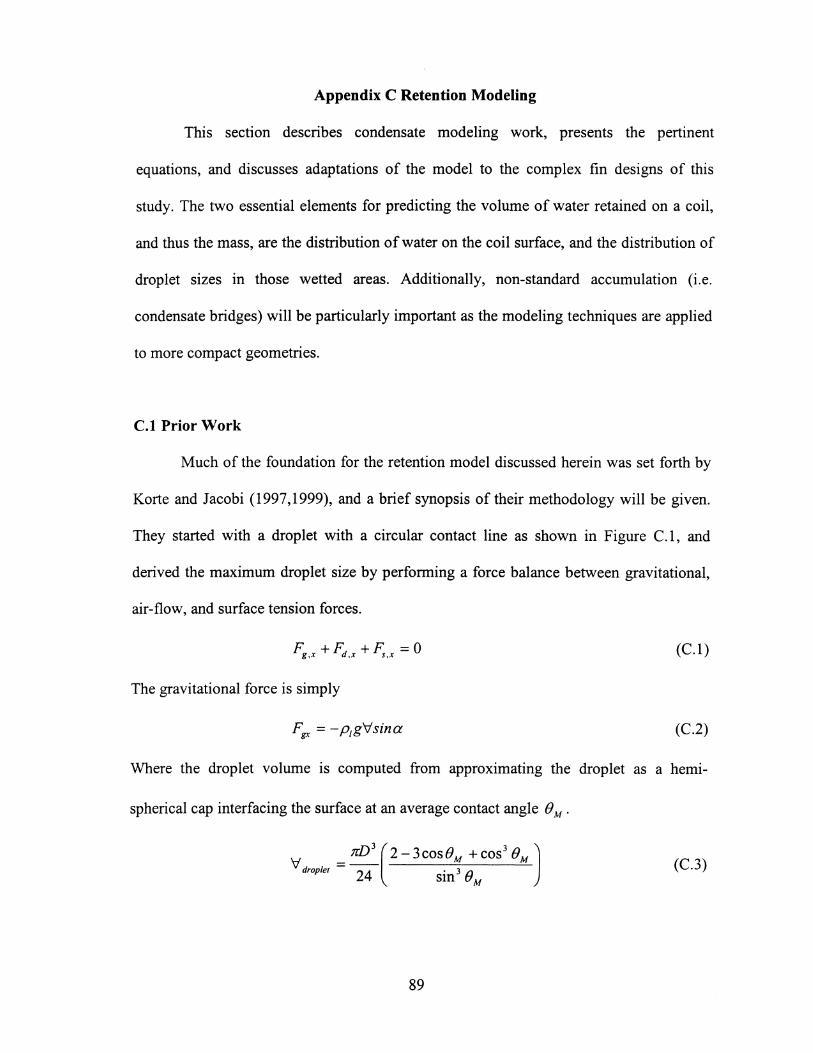
Appendix C Retention Modeling

This section describes condensate modeling work, presents the pertinent

equations, and discusses adaptations of the model to the complex fin designs of this

study. The two essential elements for predicting the volume of water retained on a coil,

and thus the mass, are the distribution of water on the coil surface, and the distribution of

droplet sizes in those wetted areas. Additionally, non-standard accumulation (i.e.

condensate bridges) will be particularly important as the modeling techniques are applied

to more compact geometries.

C.l Prior Work

Much of the foundation for the retention model discussed herein was set forth by

Korte and Jacobi (1997,1999), and a brief synopsis of their methodology will be given.

They started with a droplet with a circular contact line as shown in Figure C.1, and

derived the maximum droplet size by performing a force balance between gravitational,

air-flow, and surface tension forces.

Fg,x + Fd,x + F.,x = 0 (C.1)

The gravitational force is simply

(C.2)

Where the droplet volume is computed from approximating the droplet as a hemi-

spherical cap interfacing the surface at an average contact angle () M •

v = 1fl)3 (2 -3COS()M + cos3 ()M J droplet 24 . 3 () sm M

(C.3)

89

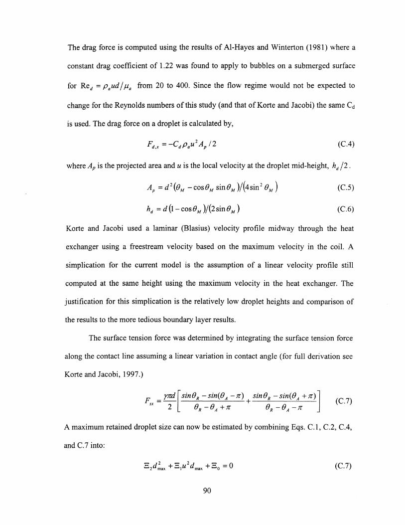
The drag force is computed using the results of AI-Hayes and Winterton (1981) where a

constant drag coefficient of 1.22 was found to apply to bubbles on a submerged surface

for Red = Paud / fLa from 20 to 400. Since the flow regime would not be expected to

change for the Reynolds numbers of this study (and that of Korte and Jacobi) the same Cd

is used. The drag force on a droplet is calculated by,

(C.4)

where Ap is the projected area and u is the local velocity at the droplet mid-height, hd /2.

(C.S)

(C.6)

Korte and Jacobi used a laminar (Blasius) velocity profile midway through the heat

exchanger using a freestream velocity based on the maximum velocity in the coil. A

simplication for the current model is the assumption of a linear velocity profile still

computed at the same height using the maximum velocity in the heat exchanger. The

justification for this simplication is the relatively low droplet heights and comparison of

the results to the more tedious boundary layer results.

The surface tension force was determined by integrating the surface tension force

along the contact line assuming a linear variation in contact angle (for full derivation see

Korte and Jacobi, 1997.)

A maximum retained droplet size can now be estimated by combining Eqs. C.1, C.2, C.4,

and C.7 into:

(C.7)

90

where,

.... -..... 1-PaCAOM -cosOM sin OM )

Ssin 2 OM

(e.S)

(e.9)

(e.1O)

Korte and Jacobi used the ideas developed by Graham (1969) to calculate the

droplet size distribution based on the maximum droplet diameter. Graham conducted

detailed photographic studies of condensation and divided the droplets into two different

groups and used the following power-law fits.

for 10,urn < d < 0.2dmax (e.lla)

for 0.2 dmax < d < dmax (e.llb)

where &V is the number of drops of diameter cL+O.2d per cm2• Through digital image

analysis the constants BJ and B2 were determined to be 2.042(106) /J.m1.73/cm2 and

4.467(109) /J.m2.8/cm2 respectively. Equation C.ll is then recast into a form for the

number of droplets a certain diameter per unit area by using !::.d = 0.4/).}/ .

n(d)=5.l 04(1 06)d"2.73

n(d)=1.117(lOJo)d"3.8

for 1O,urn < d < O.2dmax

for 0.2 dmax < d < dmax

(e.12a)

(C.12b)

The total mass of condensate on a heat exchanger surface can now be calculated by

integrating over all droplet diameters over the entire surface.

M = Pw f fn(~)V(~)d~dA (e.13) Ard

91

Korte and Jacobi (1999) used the model to successfully predict the quantity of

retained condensate on a plain-fin-and-tube heat exchanger with a fin spacing of 6.35

mm, but did not predict the retention for a heat exchanger with a fin spacing of3.18 mm.

Korte and Jacobi concluded interactions between the fins become at smaller fin spacings,

and their model does not account for any fin interactions. Yin and Jacobi (2000) added to

the model by including condensate bridges between fins at the fin-tube junction. The

model of Yin and Jacobi overpredicted the retention for a heat exchanger with a fin

spacing of 2.18 mm, and again it was concluded that interactions between droplets was

changing the distribution of water on the surface.

C.2 Adaptations

The focus of the modeling efforts for the studied automotive evaporator coils is to

attempt to use the model in its current form by separating the heat transfer surface into

four different areas with different orientations and restrictions. While this will still fall

short of accounting for interactions between droplets on adjacent fins, it will show the

applicability of the modeling ideas and give some additional insight into condensate

retention.

The studied coils have vertical, inclined, and horizontal surfaces. The tubes and

the fin-tube interface are vertical. The louver surfaces are inclined at the louver angle.

The turnaround section and the fin area between the louver-end and the tube wall is

horizontal. Each of these areas are treated seperately and slightly different. The mass of

retained condensate is predicted at face velocities of 1.0 to 2.25 mis, encompassing the

tested range of the wind tunnel retention tests. The force balance was used to compute

92

maximum droplet size was altered to investigate the possibility of droplet detachment

from gravity on the underside of the fin surface. It was found that a droplet is removed

from the surface by flow forces prior to gravity for all cases-a result that is especially

dependent on contact angles. The actual size of the droplets on the different surface

sections are constrained by geometry (the smallest computed dmax was 3.3 mm), and two

different ideas were pursued to account for this. The first is to simply set dmax equal to

largest possible droplet size such as louver pitch for the louver area and fin pitch for the

vertical area. However, this artificially modifies the distribution functions-the number

of drops calculated for example at 0.2 mm is dependent on the maximum droplet size

which should be derived from the surface conditions not size. Furthermore, by setting

dmax all dependency on air velocity is lost, which is not accurate for the tested coils. A

more logical approach (and the adopted one) is to compute the maximum droplet size in

the normal fashion and adjust Equation C.13 to integrate only up to maximum allowable

droplet size. Any droplets that are bigger are assumed to be retained in a different manner

or shed. The constraints on the sizes in the different sections are based on observations of

fin stock in the condensate visualization glove-box. It was observed that a droplet larger

than the louver pitch can remain on a louver by being non-axisymmetric.

Table C.l displays the relative area percentages of each of the different sections

and the constraints on dmax. Table C.2 is a summary of the results for applying the model

to Coil 4 showing the mass per unit area for each of the different sections and the total

predicted mass. The model prediction is compared to the experimentally measured value

graphically in Figure C.2, and the EES code is shown in Table C.3.

93

Figure C.2 shows the model underpredicted the retained mass at all frontal

velocities, an opposite trend than observed by Yin and Jacobi (2000) and Kim and Jacobi

(2000). In both those studies the authors concluded interactions between droplets on

adjacent fins caused the discrepancy. A droplet that is shed on one fin and sweeps along

the fin surface could coalesce with a large droplet on a neighboring fin and cause

premature sweeping on that fin, thus decreasing the actual mass by a mechanism not

captured by the model. In this study, the likely cause for the underprediction is bridging

between fins and louvers. The droplets that were larger than the constraint were simply

discarded. It is logical that these large drops would be the first to form bridges. The trend

in Figure C.2 that at higher velocities the prediction and measured quantities are closer

also supports this idea. At higher velocites there should be less bridging as flow forces

clear out the bridges (though this phenomenon has not been experimentally observed in

this study it is logical).

The model developed by Korte and Jacobi has been adapted and applied to a heat

exchanger tested in this study. The model correctly predicts the trends and is within 12%

of the measured value throughout the tested velocity range. The model was also applied

to Coil 5 and underpredicted the retention by 30-40%, a result that does not signify

failure of the model, but rather emphasizes the importance of condensate bridging to the

problem. Coil 5 was concluded to have a larger relative amount of condensate bridging

than Coil 4. The model does not yet include the physics of bridging or the influence of

the vertical variation in condensate retention discussed in Chapter 4, but the limited

succes in applying it to a vastly different goemetry than it was originally developed for

definitely displays its robustness.

94

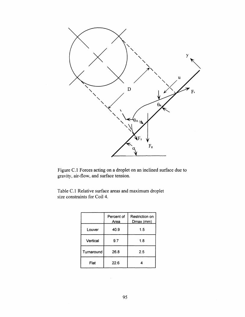
y

Figure C.I Forces acting on a droplet on an inclined surface due to gravity, air-flow, and surface tension.

Table C.I Relative surface areas and maximum droplet size constraints for Coil 4.

Percent of Restriction on Area Dmax (mm)

Louver 40.9 1.5

Vertical 9.7 1.8

Turnaround 26.8 2.5

Flat 22.6 4

95

"

Table C.2 Summary of model results for Coil 4.

Mass per unit area (g/mA2) Total Area 2.54 (mA2)

Velocity Vertical Louver Turnaround Flat

Total Mass (rn/s) (g)

1 65.1 50.5 82.9 180.7 228.7

1.25 65.3 50.8 78.4 164.8 216.9

1.5 65.6 51.1 76.2 153.6 209.4

1.75 65.8 51.5 75.2 145.1 204.3

2 66.1 52.0 74.8 138.4 200.8

2.25 66.5 52.5 74.9 133.0 198.4

300 r i j

- - - - - Model Prediction ~

J lc. Coil 4

~ I-- l-S l.. 'C

250 ~ j CI) C lc.

S &! .. .. .. lc. .. !a ......... lc.

CIS

200 ~ ......

lc. ~ ::! -- ... ---- ---- --- -1 S

1 0 I-

..j

~

150 0.5 1 1.5 2 2.5

Face Velocity (m/s)

Figure C.2 Measured and predicted values of steady-state condensate retention for Coil 4

96

EES program to calculate maximum droplet diameter and mass of water per unit area"

theta_a = 64*(PI/180) {advancing contact angle in radians} theta_r = 44.0*(PI/180) {receding contact angle in radians} alpha = alpha_d*(PI/180) {angle between fin surface normal and gravity in radians} u_max = u_a/.642 {air-side face velocity, m/s} Cs = 0.00181 {interfin spacing in m} rho = DENSITY(Water, T=20, X=O.O) {density of liquid water, kg/m"3} rho_a = DENSITY (Air, T=2S, P=101) {density of air, kg/m"3} sigma = 0.072 {surface tension, N/m} 9 = 9.8 {gravitational acceleration, m/s"2} C_d = 1.22 {drag coefficient per AI-Hays and Winterton} theta = (theta_a+theta_r)/2 {Average contact angle}

{Force Balance to find d _ max}

XCO=(xLOa+xLOb)*sigma*PI/2 xLOa=(sin(theta_r)-sin(theta_a-PI» / (theta_r - theta_a + PI)

xLOb=(sin(theta_r)-sin(theta3+PI»/ (theta_r - theta_a - PI) XC1=-rho_a*C_d*(theta - cos(theta)*sin(theta»/2 XC2=-( (2-3*cos(theta )+cos(theta)/\ 3)/( sin(theta)'" 3) )*rho*g*PI*sin( alpha )/24

y=d_m*(1-cos(theta»/4 u=u_max*(2*y/Cs) {simplification to the model of Korte and Jacobi}

XC2*(d_m)"'2 + XC1*(d_m)*u/\2 + XCO = 0 d_max=d_m* 1e6

{Integration of droplet size distribution functions}

{d_m is maximum diameter in m} {d_max is maximum diameter in microns}

n_s=(S.104e06)*( d_s)/\( -2.73) n_b=(1.117e10)*( d_b )/\( -3.80)

{number of droplets with d<.2d_max, percm"2} {number of droplets with d>.2d_max, per cm"2}

V _s=(PI*d_s/\ 3)*( (2-3*cos(theta )+cos(theta)'" 3)/(sin(theta)'" 3) )/24 {small droplet volume, microns"3}

V _b=(PI*d_b/\ 3)*( (2-3*cos(theta)+cos(theta)'" 3)/(sin(theta)'" 3) )/24 {big droplet volume, microns"3}

VT_s=INTEGRAL(n_s*V_S, d_s, 10,d_max/S) {total d_s volume in microns"3 per cm"2}

VT _b=INTEGRAL( n_b*V _b, d_b, d_max/S, d_max_constrained) {total d_b volume in microns"3 per cm"2 with max drop size constrained}

MpA=rho*(VT_s+VT_b)*(le-ll) {total retention in g/m"2}

Table C.3 EES code for computing mass per unit area for different surfaces.

97

References

AI-Hayes, RAM. and Winterton, R H. S., 1981, "Bubble Diameter on Detachment in Flowing Liquids," Int. J. Heat Mass Transfer, Vol. 24, pp. 223-230

ARl, 1981, Standardfor Forced-Circulation Air-Cooling and Air-Heating Coils, ARl-410.

Beers, Y, 1953, Introduction to the Theory of Error, Addison-Wesley Pub. Co., Cambridge, MA

Bettanini, E., 1970, "Simultaneous Heat and Mass Transfer on a Vertical Surface," International Institute of Refrigeration Bulletin, Vol. 70, pp. 309-317.

Briggs, D. E. and Young, E. H., 1969, "Modified Wilson Plot Techniques for Obtaining Heat Transfer Correlations for Shell and Tube Heat Exchangers," Chemical Engineering Progress Symposium Series, No. 92, Vol. 65, pp. 35-45.

Eckels, P. W., and Rabas, T. J., 1987, "Dehumidification: On the Correlation of Wet and Dry Transport Processes in Plate Finned-Tube Heat Exchangers," Journal of Heat Transfer, Vol. 109, pp. 575-582.

Elmahdy, A. H., 1975, "Analytical and Experimental Multi-Row, Finned-Tube Heat Exchanger Performance During Cooling and Dehumidification Processes," Ph.D. Dissertation, Carleton University, Ottawa, Canada.

Graham, c., 1969, "The Limiting Heat Transfer Mechanisms of Drop wise Condensation," PhD thesis, Massachusetts Institute of Technology, MA

Guillory, 1. L., and McQuiston, F. c., 1973, "An Experimental Investigation of Air Dehumidification in a Parallel Plate Heat Exchanger," ASH RAE Transactions, Vol. 79(2), pp. 146-151.

Ha, S., Kim, C., Ahn, S. and Dreitser, G. A, 1999, "Hydraulic Performance of Wet-FinAnd-Tube Heat Exchanger for Various Wettability Surfaces," Proceedings o/the International Conference on Compact Heat Exchangers and Enhancement Technology for the Process Industries, RK Shah, Ed., pp 463-470.

Hong, K, 1996, "Fundamental Characteristics of Dehumidifying Heat Exchangers with and without Wetting Coatings," PhD thesis, Pennsylvania State University, P A

Huang, L. 1., and Shah, R K, 1991, "Assessment of Calculation Methods for Efficiency of Straight Fins of Rectangular Profile, "Advances in Heat Exchanger Design, Radiation, and Combustion, ASME-HTD-Vol. 182, pp. 19-30.

Incoprera, F. P. and DeWitt, D. P., 1990, Fundamentals of Heat and Mass Transfer, 3rd

ed., John Wiley & Sons, New York, NY.

98

Jacobi, A M., and Goldschmidt, V. W., 1990, "Low Reynolds Number Heat and Mass Transfer Measurements of an Overall Counterflow, Baffled, Finned-Tube, Condensing Heat Exchanger," International Journal of Heat and Mass Transfer, Vol. 33, pp. 755-765.

Jasper, J. J., 1972, "The Surface Tension of Pure Liquid Compounds," J Phys. Chern. Ref Data, Vol. 1, pp. 841-1010.

Kakac, S., Shaw, R K., and Aung, W., 1987, Handbook of Single-Phase Convective Heat Transfer, John Wiley & Sons, New York, NY.

Kearney, S., and Jacobi, AM., 1996, "Local Convective Behavior and Fin Efficiency in Shallow Banks of Inline and Staggered, Annularly Finned Tubes", Journal of Heat Transfer, Vol. 118, pp. 317-326.

Kim, G. J., and Jacobi, AM., 2000, "Condensate Accumulation Effects on the Air-side Thermal Performance of Slit-fin Surfaces," Masters thesis, University of Illinois Urbana-Champaign, IL.

Kline, S. J., and McClintock, F. A, 1953, "Describing Experimental Uncertainties in Single Sample Experiments," Mechanical Engineering, Vol. 75, pp. 3-8.

Korte, C. M., and Jacobi, AM., 1997, "Condensate Retention and Shedding Effects on Air-Side Heat Exchanger Performance," ACRC-TR132, University of Illinois at Urbana-Champaign, IL.

Korte, C. M., and Jacobi, AM., 1999, "Condensate Retention and Shedding Effects on the Air-Side Performance of Plain-Fin-and-Tube Heat Exchangers: Retention and Modeling," Journal of Heat Transfer, Vol. 12.

McLaughlin, W.J. and Webb, RL., 2000a, "Condensate Drainage and Retention in Louver Fin Automotive Evaporators," Proceedings of the SAE International Congress, Detroit, MI, March 3-6.

McLaughlin, W.J. and Webb, RL., 2000b, "Wet Air Side Performance of a Louver Fin Automotive Evaporator," Proceedings of the SAE International Congress, Detroit, MI, March 3-6.

McQuiston, F. c., 1976, "Heat, Mass, and Momentum Transfer in a Parallel Plate Dehumidifying Exchanger," ASHRAE Transactions, Vol. 82(2), pp. 87-107.

McQuiston, F. c., 1978a, "Correlation of Heat, Mass, and Momentum Transport Coefficients for Plate-Fin-Tube Heat Transfer Surfaces with Staggered Tubes," ASHRAE Transactions, Vol. 84(1), pp. 294-308.

McQuiston, F. c., 1978b, "Heat, Mass and Momentum Transfer Data for Five Plate-FinTube Heat Transfer Surfaces," ASHRAE Transactions, Vol. 84(1), pp. 266-293.

99

Osada, H., et al., 1999, "Experimental Analysis for Enhancing Automotive Evaporator Fin Performance," Proceedings of the International Conference on Compact Heat Exchangers and Enhancement Technology for the Process Industries, R.K. Shah, Ed., pp. 439-445.

Rohsenow et aI., 1985, Handbook of Heat Transfer Applications, 2nd Ed., McGraw-Hill, New York, NY.

Tree, D., and Helmer, W., 1976, "Experimental Heat and Mass Transfer Data for Condensing Flow in a Parallel Plate Heat Exchanger," ASHRAE Transactions, Vol. 82(1), pp. 289-299.

Uv, E. H., and Sonju, O. K., 1992, "Heat Transfer Measurements of Circular Finned Tubes With and Without Partial Condensation," Institute of Chemical Engineers Symposium Series No. 129, Vol. 1, pp. 295-302.

Wang C.c., et al., 1994, "Experimental Study of Heat Transfer Characteristics of Automotive Evaporators," ASH RAE Transactions, Vol. 100 part 2, pp. 575-582

Wang, C. c., Hsieh, Y. c., and Lin, Y, T., 1997, "Performance of Plate Finned Tube Heat Exchangers Under Dehumidifying Conditions," Journal of Heat Transfer, Vol. 119, pp. 109-107.

White, F. M., 1991, Viscous Fluid Flow, 2nd Ed., McGraw-Hill, New York, NY.

Wilson, E. E., 1915, "A Basis for Rational Design of Heat Transfer Apparatus," Transactions of the ASME, 37, pp. 47-70.

WU, G., and Bong, R. C., 1994, "Overall Efficiency of a Straight Fin With Combined Heat and Mass Transfer," ASHRAE Transactions, Vol. 89, pp. 367-374.

Yin, J., and Jacobi, A.M., 2000, "Condensate Retention Effects on the Air-side Heat Transfer Performance of Plain and Wavy-louvered Heat Exchangers," Masters thesis, University of Illinois Urbana-Champaign, IL

Yoshii T., Yamamoto, M., and Otaki, T., 1973, "Effects of Drop wise Condensate on Wet Surface Heat Transfer of Air Cooling Coils," Proc. 13th Int. Congress of Refrigeration, pp. 285-292.

100

Documents

Condensate Retention Effects on the Air-Side Heat Transfer