Embed Size (px)
Citation preview

Concurrent Range Reporting in Two-Dimensional Space
Peyman Afshani∗ Cheng Sheng† Yufei Tao† Bryan T. Wilkinson∗‡
Abstract
In the concurrent range reporting (CRR) problem, the input is L disjoint sets S1, ..., SL of points inRd with a total of N points. The goal is to preprocess the sets into a structure such that, given a queryrange r and an arbitrary set Q ⊆ 1, ..., L, we can efficiently report all the points in Si ∩ r for eachi ∈ Q. The problem was studied as early as 1986 by Chazelle and Guibas [9] and has recently re-emergedwhen studying higher-dimensional complexity of orthogonal range reporting [2, 3].
We focus on the one- and two-dimensional cases of the problem. We prove that in the pointer-machine model (as well as comparison models such as the real RAM model), answering queries requiresΩ(|Q| log(L/|Q|) + logN + K) time in the worst case, where K is the number of output points. In onedimension, we achieve this query time with a linear-space dynamic data structure that requires optimalO(logN) time to update. We also achieve this query time in the static case for dominance and halfspacequeries in the plane. For three-sided ranges, we get close to within an inverse Ackermann (α(·)) factor:we answer queries in O(|Q| log(L/|Q|)α(L)+logN+K) time, improving the best previously known querytimes of O(|Q| log(N/|Q|) +K) and O(2LL+ logN +K). Finally, we give an optimal data structure forthree-sided ranges for the case L = O(logN).
∗MADALGO, Aarhus University, Denmark, peyman,[email protected]. MADALGO is a center of the Danish NationalResearch Foundation.†Department of Computer Science and Engineering, Chinese University of Hong Kong, Hong Kong,
csheng,[email protected]. Supported by grants GRF 4165/11, GRF 4164/12, and GRF 4168/13 from HKRGC.‡Supported by the Natural Sciences and Engineering Research Council of Canada (NSERC).
1
1
2
3
4
5
6
7
8
9
10
11
12
13
14
15
16
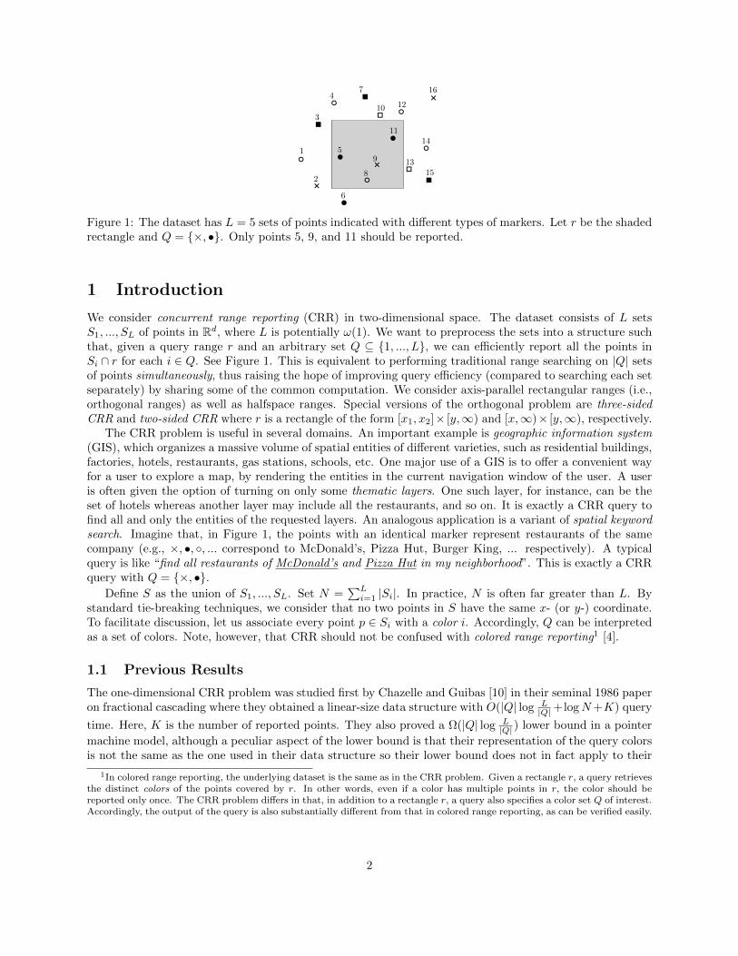
Figure 1: The dataset has L = 5 sets of points indicated with different types of markers. Let r be the shadedrectangle and Q = ×, •. Only points 5, 9, and 11 should be reported.
1 Introduction
We consider concurrent range reporting (CRR) in two-dimensional space. The dataset consists of L setsS1, ..., SL of points in Rd, where L is potentially ω(1). We want to preprocess the sets into a structure suchthat, given a query range r and an arbitrary set Q ⊆ 1, ..., L, we can efficiently report all the points inSi ∩ r for each i ∈ Q. See Figure 1. This is equivalent to performing traditional range searching on |Q| setsof points simultaneously, thus raising the hope of improving query efficiency (compared to searching each setseparately) by sharing some of the common computation. We consider axis-parallel rectangular ranges (i.e.,orthogonal ranges) as well as halfspace ranges. Special versions of the orthogonal problem are three-sidedCRR and two-sided CRR where r is a rectangle of the form [x1, x2]× [y,∞) and [x,∞)× [y,∞), respectively.
The CRR problem is useful in several domains. An important example is geographic information system(GIS), which organizes a massive volume of spatial entities of different varieties, such as residential buildings,factories, hotels, restaurants, gas stations, schools, etc. One major use of a GIS is to offer a convenient wayfor a user to explore a map, by rendering the entities in the current navigation window of the user. A useris often given the option of turning on only some thematic layers. One such layer, for instance, can be theset of hotels whereas another layer may include all the restaurants, and so on. It is exactly a CRR query tofind all and only the entities of the requested layers. An analogous application is a variant of spatial keywordsearch. Imagine that, in Figure 1, the points with an identical marker represent restaurants of the samecompany (e.g., ×, •, , ... correspond to McDonald’s, Pizza Hut, Burger King, ... respectively). A typicalquery is like “find all restaurants of McDonald’s and Pizza Hut in my neighborhood”. This is exactly a CRRquery with Q = ×, •.
Define S as the union of S1, ..., SL. Set N =∑Li=1 |Si|. In practice, N is often far greater than L. By
standard tie-breaking techniques, we consider that no two points in S have the same x- (or y-) coordinate.To facilitate discussion, let us associate every point p ∈ Si with a color i. Accordingly, Q can be interpretedas a set of colors. Note, however, that CRR should not be confused with colored range reporting1 [4].
1.1 Previous Results
The one-dimensional CRR problem was studied first by Chazelle and Guibas [10] in their seminal 1986 paperon fractional cascading where they obtained a linear-size data structure with O(|Q| log L
|Q|+logN+K) query
time. Here, K is the number of reported points. They also proved a Ω(|Q| log L|Q| ) lower bound in a pointer
machine model, although a peculiar aspect of the lower bound is that their representation of the query colorsis not the same as the one used in their data structure so their lower bound does not in fact apply to their
1In colored range reporting, the underlying dataset is the same as in the CRR problem. Given a rectangle r, a query retrievesthe distinct colors of the points covered by r. In other words, even if a color has multiple points in r, the color should bereported only once. The CRR problem differs in that, in addition to a rectangle r, a query also specifies a color set Q of interest.Accordingly, the output of the query is also substantially different from that in colored range reporting, as can be verified easily.
2

algorithm (see Section 2 for more details). By applying dynamic fractional cascading [9, 16], this methodsupports an update in O(logN) time, but the query cost becomes O(|Q| log L
|Q| log logN + logN +K).
In two dimensions, a trivial solution is to issue |Q| individual range reporting queries, one on each colorin Q. Using a structure of Chazelle [8], this gives a data structure for the two-dimensional CRR problemthat uses O(N logN/ log logN) space2 and answers a query in O(|Q| log N
|Q| + K) time. If all queries are
three-sided, the space can be lowered to linear by resorting to the priority search tree [15], while the querycost remains the same. The only non-trivial solutions for CRR in dimensions two and higher were givenby Afshani et al. [2] (see also [3]). They considered a special instance of three-sided CRR, which has anadditional constraint that Q can be selected from only a number M ≤ 2L of possible choices. They gave alinear-space structure that answers a (three-sided) query in O(ML+logN+K) time. While this adequatelyserves the purposes in [2], in our context where Q can be any subset of [L] (notation [x] represents the setof integers 1, ..., x), the query time becomes O(2LL+ logN +K).
1.2 Our Results
Our main contribution is to show that almost optimal results can also be obtained for two-dimensional CRRproblems. Our bounds involve some sublogarithmic functions which we now define. Let αp(x) for p ≥ 1 bea family of functions that are defined for x ≥ 1. In the base case p = 1, α1(x) = x − 2. For p > 1, we let
αp(x) = mini | i ≥ 1 ∧ α(i−1)p−1 (x) ≤ 2. Here, α
(i−1)p−1 is the identity function composed with i− 1 instances
of the αp−1 function. In this way, α2(x) = dn/2e, α3(x) = max1, dlog xe, α4(x) = max1, dlog∗ xe andso on. Let α(x) be minp | αp(x) ≤ 3 so that it is asymptotically equivalent to the inverse Ackermannfunction [12].
Theorem 1. Given N points in R2 divided into L disjoint sets, we can construct a pointer-machine structurethat answers three-sided CRR queries and has one of the following pairs of bounds (K is the size of the queryresult):
1. O(Nαp(N/L)) space and O(|Q| log(L/|Q|) + logN +K) query time, for any constant p ≥ 3;
2. O(N) space and O(|Q|(log(L/|Q|) + logαp(N/L)) + logN +K) query time, for any constant p ≥ 3; or
3. O(N) space and O(|Q| log(L/|Q|)α(N/L) + logN +K) query time.
Each of these data structures require O(S(N) logN) preprocessing time, where S(N) is the data structure’sspace bound.
Our data structure makes extensive use of a space-saving technique for three-sided range searching ap-pearing as early as the work of [17] that involves dividing the point set into slabs and building data structuresfor the points within each slab and a data structure on representative points from each slab.
Additionally, we obtain a number of other results that enhance our understanding of the CRR problems:We consider two different methods of specifying the query colors as the previous papers had not done this ina satisfactory way (e.g., consider the peculiar aspect of Chazelle and Guibas’s lower bound [9]). We prove asignificantly more involved lower bound and provide some other reductions that ultimately show the differentformulations of the query colors are in fact equivalent. We also observe that the Ω(|Q| log(L/|Q|)+logN+K)query lower bound also holds in the comparison model, which means our results are almost optimal in otherfundamental models such as the real RAM model.
The data structure of Afshani et al. [2] achieves linear space and O(logN + K) query time for the caseL ≤ log logN − log log logN . In Section 6, we give a data structure that achieves these same bounds fora broader special case of L = O(logN). Our data structure uses persistence to transform a dynamic 1dsolution based on an interval tree into a static three-sided solution. If we use either of these data structuresfor small settings of L and the data structure of Theorem 1 for larger L, then we can rewrite the bounds
2All logarithms in this paper have base 2. Furthermore, we follow the convention that every logarithm returns a value atleast 1, by defining log x = max1, log2 x.
3
of Theorem 1 so that, for p ≥ 4, αp(N/L) becomes αp(L) and α(N/L) becomes α(L). This is because, forp ≥ 4 and L > log logN − log log logN , αp(N/L) = O(αp(L)) and α(N/L) = O(α(L)).
By standard (range tree) techniques, Theorem 1 implies that a general (four-sided) CRR query can besettled with the same query cost, after increasing space by a factor of O(logN). When restricted to two-sidedranges, and also for halfspace ranges, we obtain linear space and O(|Q| log L
|Q| + logN +K) query time. We
also present an optimal dynamic one-dimensional structure.
Theorem 2. Given N values in R divided into L disjoint sets, there is a dynamic structure that requiresO(N) space, and answers a one-dimensional CRR query in O(|Q| log L
|Q| + logN +K) time, where K is the
size of the query result. The structure supports insertions and deletions in O(logN) amortized time.
We sometimes need to perform a concurrent lookup on a BST T indexing L keys. Given a set Q ofsorted keys, each of which is indexed by T , this operation finds the nodes in T corresponding to the keys inQ. Chazelle and Guibas [10] show that the minimum spanning tree of the |Q| output nodes in T has sizeO(|Q| log(L/|Q|)). It is then straightforward to perform a concurrent lookup in O(|Q| log(L/|Q|)) time byperforming an Euler tour of this minimum spanning tree: at each step we progress towards the least querykey that we have not yet found. Since the query keys are sorted, we always know the next least key toprogress towards.
2 Query Representation and Lower Bounds
In this section, we discuss the representation of query colors as there is a potential for ambiguity whenstudying CRR problems in a pointer machine. In fact this ambiguity has already revealed itself in theprevious work of Chazelle and Guibas [10]: when employing the fractional cascading technique, they assumethat the query colors are given as pointers to special nodes of the pointer machine but while proving theoptimality of said technique, they assume that the query colors are given instead by indices. This means intheir data structure, it is assumed that the query begins by having access to |Q| pointers (thus |Q| entrypoints into the data structure) but when proving the lower bound, they assume the query algorithm beginsby having access to one entry point. The latter is a much more restrictive starting setup for the queryalgorithm which means their data structure does not in fact fit their lower bound framework!
We explicitly define these two different (but as it turns out equivalent) query representations. In thefirst representation, the set of query colors is a sorted set of indices. We consider this the index queryrepresentation. In an alternate representation, each color i is associated with some specific node ci in thepointer-machine structure called a color node. Let C = c1, c2, . . . , cL be the set of all the color nodes. Aset of query colors is specified by a set Q ⊆ C (more precisely, Q is a set of pointers to the color nodes) thatis not necessarily sorted in any way. We call this the pointer query representation.
We first give O(L)-space and O(|Q| log(L/|Q|))-time reductions between the index and pointer queryrepresentations. We then proceed to show that there is a lower bound of Ω(|Q| log(L/|Q|)) for both queryrepresentations. Thus, these representations are equivalent in the pointer-machine model, and any datastructure for CRR with O(|Q| log(L/|Q|) + logN +K) query time is optimal in the pointer-machine model.
2.1 Query Representation Reductions
Lemma 1. Given a data structure D for CRR with the pointer query representation that requires TD querytime and SD space, there exists a data structure for CRR with the index query representation that requiresO(SD + L) space and O(TD + |Q| log(L/|Q|)) query time.
Proof. We build a BST T on the L color nodes of D based on the sorted order of the colors. Then, given asorted set of query colors Q, we find their associated color nodes in O(|Q| log(L/|Q|)) time via a concurrentlookup in T . We then query D with the color nodes.
4
Lemma 2. Given a data structure D for CRR with the index query representation that requires TD querytime and SD space, there exists a data structure for CRR with the pointer query representation that requiresO(SD + L) space and O(TD + |Q| log(L/|Q|)) query time.
Proof. We construct a color node for each color and store them in a BST T based on the sorted order of thecolors. As shown by Chazelle and Guibas [10], if we augment T with parent pointers, then we can constructthe minimum spanning tree of a set of query color nodes in O(|Q| log(L/|Q|)) time. In the same amount oftime, we perform an in-order traversal of the minimum spanning tree to recover the query colors in sortedorder. We then query D with the sorted set of query colors.
2.2 Lower Bounds
For the intex query representation, obtaining a comparison-based lower bound is straightforward: consider adataset where each Si has only one point and a query range that covers all of these points. For any specific |Q|,there are
(L|Q|)
size-|Q| subsets of [L], each of which defines a unique result. Since any query algorithm must
be able to distinguish at least as many results, it follows that Ω(log(L|Q|)) = Ω(|Q| log(L/|Q|)) comparisons
are needed. This is essentially a lower bound for a problem we call the concurrent lookup problem: given aset T of keys, store them in a data structure such that given a set Q of sorted query keys, each of which isindexed by T , find the keys in T that correspond to the keys in Q.
We now consider the pointer-machine model. In this model, the memory is a directed graph with outdegree of two (the model generalizes easily to any constant out degree as well) and each node of the graphcan store one input element. To output an element, the query algorithm must navigate the pointers to reacha cell that contains the element. While Chazelle and Guibas proved a pointer-machine lower bound [10],their lower bound assumes the colors are given as indices rather than pointers. In this way, the CRR probleminherits the difficulty of the concurrent lookup problem, which makes proving a lower bound easier. Instead,we consider the pointer query representation, which means the query algorithm begins with access to |Q|entry points to the data structure; this is in contrast to the traditional pointer machine data structures inwhich the query algorithm begins from the root of the data structure. In fact, because of this, we cannot takeadvantage of the difficulty of the concurrent lookup problem, and we must instead consider the geometry ofthe problem. Essentially, we space out many instances of the concurrent lookup problem and show that thecolor nodes cannot adequately help all instances of the problem. While simple counting arguments work toestablish a lower bound when starting from one pointer, they seem to be ineffective when starting from |Q|pointers. When the query algorithm begins from one pointer, it can only access 2O(k) different subsets ofthe memory cells by making k pointer jumps so to be able to access
(L|Q|)
sets we must have 2O(k) ≥(L|Q|)
or
k = Ω(|Q| log(L/|Q|)). On the other hand, if we give the query algorithm access to |Q| pointers, there are(L|Q|)
ways just to pick our entry points and so the counting argument is rendered completely ineffective. To
establish a lower bound for the pointer query representation, we have to work harder.
Theorem 3. Any pointer-machine data structure for CRR with the pointer query representation that uses(N/L)O(1) space, requires Ω(|Q| log(L/|Q|) + logN +K) query time.
Proof. Our bad input instance is a one-dimensional point set composed of N/L sets of size L. Each set onlycontains one point of each color and the points in the i-th set are laid consecutively in an interval Ii; theintervals are disjoint and they are also used as geometric ranges for queries. Thus, for a set Q ⊆ C of colornodes, the output size for the query range Ii is exactly |Q|. In our proof, the number of colors for all querieswill be fixed but to avoid introducing extra variables, we will continue to use |Q| to refer to this fixed value.
If logN ≥ |Q| log(L/|Q|) then there is nothing left to prove since there is a trivial Ω(logN) lower boundin the pointer-machine model. In the rest of this proof, we assume otherwise. Let G be the directed graphthat corresponds to the memory layout of the data structure: the vertices of G are memory cells and edgescorrespond to the pointers between the memory cells. G has L cells that correspond to the color nodes;the query algorithm begins the search from these cells. We say a memory cell (in G) is shallow, if it lies at
5

a depth less than log(N/L) − 2 of a color node. We say an interval I is shallow, it there are at least L/2shallow cells that store points in I. Since the number of shallow cells is less than L2log(N/L)−2 = N/4, thereare less than N/(2L) shallow intervals. We will only use non-shallow intervals for our queries so one cansafely ignore the shallow intervals in the rest of this proof.
Given a non-shallow interval I, consider the query algorithm: it starts with access to |Q| pointers andthen continues to make pointer jumps in graph G until all the cells containing the output have been accessed.We ignore the part of the output that is stored in shallow cells so for the rest of this proof, by output wemean only the points that are not stored in shallow cells (in other words, we only require the query algorithmto output elements stored in non-shallow cells).
Consider the subgraph H of G composed of memory cells that are explored at the query time and theedges that are used to visit these cells for the first time. Except for the color nodes, each vertex of H hasin-degree of exactly one (each color node has in-degree zero). So, H is a forest with |Q| arborescences3 suchthat each color node in Q is the root of one arborescence. H contains at most |Q| cells that store the outputpoints of the query. We call these the output cells. We denote the number of output cells in an arborescenceT with k(T ). Let α|Q| be the size of H which is also a lower bound on the query time. We call a subgraphof G a β-heavy hub of size r if it is an arborescence of size r with β output cells. Intuitively, our proof ideais to combine two things: one, that for every query, the subgraph H contains at least one β-heavy hub ofsize O(αβ) and two, that the number of β-heavy hubs of size O(αβ) that the graph G can use at the querytime depends on and grows as a function of α.
We set β = C log(N/L)/ log(L/|Q|), where C is a constant to be determined later. Consider an arbores-cence T in H with k(T ) > 0. Observe that T must have at least log(N/L)− 2 vertices (since its output cellsare not shallow). If a fraction (say a quarter) of all the output elements lie in arborescences T such thatk(T ) ≤ 2β, then we are good: each such arborescence uses at least an average of log(L/|Q|)/(2C) pointerjumps to output one element and thus the query time is already Ω(|Q| log(L/|Q|). Thus, assume otherwisewhich means we can afford to remove any arborescences T with k(T ) ≤ 2β and still have three quarters ofthe output elements left. After this, since the total size of all the arborescences were α|Q|, it easily followsthat there exists at least one arborescence T such that |T | ≤ 2αk(T ) with k(T ) ≥ 2β. In this case, by usingthe same technique as in [1], we can find at least one β-heavy hub of size O(αβ).
We now look at the overall structure of graph G. While the definition of a β-heavy hub only makes sensewith respect to a given query, the structure of the hub must still be embedded in graph G. This means thatG has only a limited number of different β-heavy hubs of size O(αβ). To bound this number, we can pick acell v in graph G, consider O(αβ) pointer jumps that visit O(αβ) other memory cells in G and then pick βcells out of all the visited cells to be output cells. After considering all the different possible pointer jumps,and all the different ways to pick β cells out of O(αβ) cells, it is a simple exercise (for more details see [1])to show that the number of different possible β-heavy hubs of size O(αβ) in G is S(N)2O(αβ) where S(N) isthe total space used by the data structure (S(N) is in fact the number vertices in graph G). Now, rememberthat we have at least N/(2L) non-shallow intervals so there exists a non-shallow interval I such that thereare at most S(N)2O(αβ)L/N possible β-heavy hubs of size O(αβ) that involve cells that store points of I.
We fix I as the query range and it remains to define the color set. Since I has only one point of eachcolor, output points and query colors are interchangeable (i.e., we can determine Q by a query’s set of outputpoints). To pick the set of output points, we consider the points of I that are not stored in shallow cells;by the non-shallowness of I, there are at least L/2 such points. Q is picked by randomly sampling eachsuch point with probability 2|Q|/L (remember that |Q| is a fixed parameter). The number of points thatwe consider is at least L/2, so we expect to sample |Q| colors. Now, consider a possible β-heavy hub h. Ifthe point stored at one of the output cells of h is not sampled, then h is not useful since it cannot becomea β-heavy hub for our query. Thus, the probability that h is useful for the our query is at most (2|Q|/L)β .This implies that the expected number of β-heavy hubs that can be useful for the query is at most(
2|Q|L
)βS(N)2O(αβ) L
N.
3An arborescence is a directed tree in which there is a directed path from the root to every other node, or informally, adirected tree in which the edges are directed away from the root.
6
Since β = C log(N/L)/ log(L/|Q|), we have (|Q|/L)β = 2−C log(N/L) = (N/L)−C . To be able to answer thequery, the query should have at least one such β-heavy hub, implying(
L
N
)C−1S(N)
(N
L
)O( Cαlog(L/|Q|) )
≥ 1.
Since S(N) = (N/L)O(1), by setting C a large enough constant, it follows that we must have α = Ω(log(L/|Q|)).
Corollary 1. For L ≤√N , any pointer-machine data structure for CRR with the pointer query represen-
tation that uses polynomial space, requires Ω(|Q| log(L/|Q|) + logN +K) query time.
3 Two-Sided and Halfspace CRR
Before looking at 2d CRR, consider the concurrent version of predecessor search. In this problem we mustpreprocess L sets S1, . . . , SL of elements so that we can efficiently find the predecessor of a query element qin Si for each i in a set of query colors Q ⊆ [L]. The solution to 1d CRR of Chazelle and Guibas [10] alsosolves concurrent predecessor search in linear space and optimal O(|Q| log(L/|Q|) + logN) time.
Assume we have a data structure for traditional range reporting that, in order to answer a query, performsa single 1d predecessor search and then uses O(K) additional time to report all necessary points. Supposedfurther that the query element used in the 1d predecessor search depends only on the original query range(i.e., it does not depend on the points stored in the data structure). Observe that we can then build anefficient data structure for CRR by building this traditional data structure for each color, but performingthe predecessor searches for each query color concurrently. This concurrent predecessor search requiresO(|Q| log(L/|Q|) + logN) time, and all subsequent work is bounded by O(K).
Lemma 3. There exists a linear-space data structure for two-sided range reporting that requires, for anyquery, a single predecessor search that depends on only the query and O(K) additional time. The datastructure requires O(N logN) preprocessing time.
Proof. Given a point set S, let `1, . . . , `m be all m non-empty layers of maxima of S, such that `i containsthe maxima of S\⋃i−1j=1 `j . We store the points of each layer in a linked list in order of increasing x-coordinate(or equivalently, decreasing y-coordinate). For each layer `i, we build a catalog Ci containing the points of `ikeyed by their x-coordinates. We connect the catalogs into a path ordered by layer index to create a cataloggraph that supports fractional cascading. Proprocessing time is dominated by the construction of the layersof maxima in O(N logN) time by a simple sweep-line algorithm.
Given an query with range r = [x0,∞)× [y0,∞), we report points layer by layer, starting at `1, until wereach a layer `i such that `i ∩ r = ∅. Since the points of `i dominate the points of all further layers, for anyfurther layer `j , it must also be that `j ∩ r = ∅. When we consider some layer `i, we must report `i ∩ r. Inorder to do so, we search for the point p associated with the successor of x0 in Ci. If there is no such point,then `i ∩ r = ∅ and we are done. Otherwise, p is the highest point of `i that is to the right of x0. We reportpoints of the linked list for `i, starting from p, until we reach a point with y-coordinate less than y0.
We need to search for the successor of x0 in a path of at most O(K) catalogs in our catalog graph. Byfractional cascading, this requires a single predecessor search for x0 in the augmented catalog for C1, followedby O(K) additional work.
Lemma 3 implies an optimal two-sided CRR pointer-machine structure with linear space andO(|Q| log(L/|Q|)+logN +K) query time that can be built in O(N logN) time. There is also a linear-space data structure for2d halfspace range reporting that performs a single predecessor search followed by O(K) additional work.It is similar to the data structure of Lemma 3, but uses convex layers instead of layers of maxima. Convexlayers can also be constructed in O(N logN) time [7]. Finding a point on a convex layer in a given halfspacereduces to predecessor search over the slopes of the edges of the convex layer, using the slope of the halfspaceboundary line as the query element. Therefore, there is a linear-space data structure for 2d halfspace CRRwith O(|Q| log(L/|Q|) + logN +K) query time that can be built in O(N logN) time.
7
4 Three-Sided CRR
This section concerns the proof of Theorem 1. Recall that the dataset S has N points in R2, each of whichis associated with a color i ∈ [L]. A three-sided CRR query specifies a rectangle r = [x1, x2] × [y,∞) anda color set Q ⊆ [L], and retrieves Si ∩ r for each i ∈ Q. As mentioned in Section 1, there is a simplelinear-space data structure for three-sided CRR based on priority search trees that requires suboptimalO(|Q| log(N/|Q|) + K) query time. Priority search trees can be built in O(N logN) time, which is thusthe data structure’s preprocessing time. Note, that in the special case where N = O(L), this naive datastructure is actually optimal. We will use this data structure as the base case for a few recursive structures.We will also use the two-sided solution of Section 3 as a black box. For each new data structure in thissection, the analysis of the data structure’s preprocessing time is identical to that of its space consumption,except that the preprocessing bound has an extra multiplicative O(logN) factor. This extra factor is simplypropagated from the naive three-sided data structures and optimal two-sided data structures that we use asblack boxes.
Lemma 4. There exists a data structure for three-sided CRR that requires O(N log(N/L)) space andO(|Q| log(L/|Q|) + logN +K) query time.
Proof. As mentioned in Section 3, using a range tree and our optimal two-sided solution, we can create anO(N logN)-space data structure for three-sided queries with optimal query time. By modifying the tree sothat it has fat leaves of size O(L), and building the naive data structure for three-sided CRR in these leaves,we reduce space to O(N log(N/L)) and retain optimal query time.
Note that the data structure of Lemma 4 requires O(Nα3(N/L)) space. We now give a technique thatreduces space from O(Nαp(N/L)) to O(Nαp+1(N/L)).
Theorem 4. There exists a data structure for three-sided CRR that requires O(Npαp(N/L)) space andO(|Q|p log(L/|Q|) + logN +K) query time, for any p ≥ 3.
The data structure of Theorem 4 for parameter p = q recursively uses the data structure for p = q − 1.Let Sp(N) and Tp(N) be the space and query time, respectively, required by our data structure for parameterp. In the base case p = 3, we simply use the data structure of Lemma 4, so we have S3(N) = O(Nα3(N/L))and T3(N) = O(|Q| log(L/|Q|) + logN +K), as required. We now wish to prove the theorem for p = q > 3.
We construct a range tree T on the x-coordinates of points so that each node u is associated with anx-range I(u) and the x-ranges of the children of u partition I(u) such that an equal number of points of S liein each child x-range. The children of u are ordered based on the natural ordering of their x-ranges. Let Sube the points of S which lie in I(u). Our range tree T has a different fanout parameter at each level. If the
root of T is at level 1, then a node u at level i is associated with an x-range I(u) that contains Lα(i−1)q−1 (N/L)
points. Our range tree T has fat leaves of size at most 2L at level αq(N/L).In each fat leaf u, we store the naive three-sided CRR data structure on Su, which is optimal for
|Su| = O(L) points. In each non-root node u we build a two-sided CRR data structure D+u on Su for
queries of the form [x,∞)× [y,∞) and (by mirroring Su) another data structure D−u for queries of the form(−∞, x]× [y,∞). Now, consider an internal node u. We build a BST Bu on the set of left boundaries of the
x-ranges of the children of u. Finally, we build a data structure D||u on Su for three-sided ranges of the form
[x1, x2)× [y,∞) where x1, x2 ∈ Bu. We call these aligned queries.
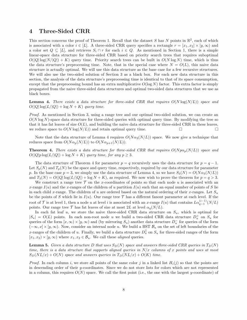
Lemma 5. Given a data structure D that uses SD(N) space and answers three-sided CRR queries in TD(N)time, there is a data structure that supports aligned queries in N/x columns of x points and uses at mostSD(NL/x) +O(N) space and answers queries in TD(NL/x) +O(K) time.
Proof. In each column i, we store all points of the same color j in a linked list Hi(j) so that the points arein descending order of their y-coordinates. Since we do not store lists for colors which are not representedin a column, this requires O(N) space. We call the first point (i.e., the one with the largest y-coordinate) of
8
r+ r−r||
Figure 2: The points of Su are partitioned into columns. Head points (depicted large) are the highest pointsof each linked list. The query range is decomposed into two-sided queries in the outer columns and a singlealigned query.
each list Hi(j) a head point. See Figure 2. We store all head points in data structure D, which requires atmost SD(NL/x) space.
Given an aligned query with range r = [x1, x2] × [y,∞) and color set Q, we forward the query to thedata structure containing only head points, so that in TD(NL/x) time we have reported all appropriatehead points. Consider any non-head point that should be reported. Then, every prior point in its linked listHi(j) must also be reported. The points of Hi(j) that lie in r thus form a prefix of Hi(j). We know that thehead point for Hi(j) was reported. So, for every head point that was reported, we scan its linked list andreport its points until we reach a point that is outside of r. We charge this additional work to the outputsize.
The data structure D||u is that of Lemma 5, where x = Lα
(i)q−1(N/L) and D is the data structure of
Theorem 4 with parameter p = q − 1.For the space analysis, we strengthen our claimed space bound to Sp(N) ≤ cNpαp(N/L) for a sufficiently
large constant c. Our induction hypothesis gives that Sq−1(N) ≤ cN(q − 1)αq−1(N/L). Consider a singlelevel i of T . Each node u in level i requires at most Sq−1(|Su|L/x)+c|Su| space. Here the c|Su| term includesthe linked lists of Lemma 5, as well as the data structures D+
u , D−u , and Bu. By the induction hypothesisand simple arithmetic, the total space for u is less than or equal to c|Su|q. The total space required at leveli is thus at most cNq, since every point in S lies in the x-range of exactly one node at level i. Since T hasαq(N/L) levels, the total space for T is cNqαq(N/L), as required.
We now show how queries are answered. Given a query with range r = [x1, x2] × [y,∞) and colorset Q, we begin by finding the lowest node u in T such that x1, x2 ∈ I(u). We do so by predecessorsearch for x1 and x2 in Bv for each ancestor v of u, starting from the root of T . This process takesO(∑v(1 + log(|Bv|))) = O(αq(N/L) + logN) = O(logN) time.
If u is a leaf, we query the naive three-sided data structure stored at u with range r and color set Q andwe are done in O(|Q| log(L/|Q|) + logN + K) time. If u is an internal node, then we know that u has twodifferent children v1 and v2 such that x1 ∈ I(v1) and x2 ∈ I(v2). Let x′1 be the left boundary of the x-rangeof the right sibling of v1 and let x′2 be the left boundary of I(v2). We decompose r into three subrangesr+ = [x1, x
′1)× [y,∞], r|| = [x′1, x
′2)× [y,∞], and r− = [x′2, x2]× [y,∞], as shown in Figure 2.
Amongst the points of Sv1 , the range r+ contains the same points as [x1,∞] × [y,∞], thus we handlethis subrange in O(|Q| log(L/|Q|) + logN + K) time via a two-sided query to D+
v1 . We can handle r−
symmetrically with a two-sided query to D−v2 . Finally, we handle r|| by recursing in D||u with the range r||.
At each level of recursion we perform O(|Q| log(L/|Q|) + logN) work that can’t be charged to the outputsize. So, the total query time is O(p(|Q| log(L/|Q|) + logN) +K).
We can reduce the O(p logN) term to O(logN) by fractional cascading. The O(p logN) term comesfrom two O(logN) time algorithms that we invoke at each of the O(p) levels of recursion: first, finding thenode u in T at which we can decompose r into an aligned query and two-sided queries, and second, the
9

two-sided CRR queries. Both of these algorithms amount to predecessor search for x1 and x2 in differentsets of elements. In finding node u we search for x1 and x2 in Bv for each ancestor v of u. The two-sidedCRR query algorithms search for x1 or x2 in layers of maxima.
We construct a global catalog graph for all O(p) levels of recursion. Each node u in a tree T at recursionlevel q is associated with a catalog Cu that contains the elements of Bu. If u is the root of T , then Cu is
linked to Cv for some node v in recursion level q + 1 that uses T in D||v . If u is not the root of T , then Cu
is instead linked to Cv where v is the parent of u. If u is an internal node, then Cu is linked to Cv where v
is the root of a tree at recursion level q − 1 in D||u as well as Cw for each child w of u. In this case, Cu is
also linked to the catalogs for the first layers of maxima in D+u and D−u . Our catalog graph thus has locally
bounded degree of 5: although there are a non-constant number of links to children, they only contributeto an increase of the locally bounded degree by one since the ranges of the catalogs of the children are alldisjoint.
An issue that we have thus far ignored is that, when we recurse, we change the query x-coordinates fromx1 and x2 to x′1 and x′2. Typically, in fractional cascading, one searches for the same query elements in everycatalog. However, it is straightforward to extend fractional cascading without penalty so that it is possibleto switch the query value to the result of a previous search in an adjacent catalog. When we recurse, this isprecisely what we need to do: x′1 and x′2 are the results of searches in Bu (now Cu) and these values become
the new query values in the root of the tree for D||u.
Now, we must count the number of catalogs that we visit to give a bound on running time. At eachlevel of the tree at each recursion level, there are a constant number of catalogs that we search and cannotcharge to the output size. Thus, the O(p logN) term is reduced by fractional cascading to O(logN) +∑pq=4O(αq(N/L)) = O(logN). This completes the proof of Theorem 4.By fixing p to a constant in Theorem 4, we obtain trade-off 1 of Theorem 1. To get the other two
trade-offs, we need one final step to reduce space to O(N).
Theorem 5. There exists a data structure for three-sided CRR that requires O(N) space and O(|Q|(p log(L/|Q|)+log(pαp(N/L))) + logN +K) query time, for any p ≥ 3.
Proof. We divide our set of points S into columns of O(Lpαp(N/L)) points. To handle queries that lieentirely within one of these columns, we build the naive data structure for three-sided queries in each col-umn. These data structures require linear space and O(|Q| log(Lpαp(N/L)/|Q|) +K) = O(|Q|(log(L/|Q|) +log(pαp(N/L))) + K) query time. To handle queries that do not lie entirely within one column, we reusethe technique of Theorem 4 to decompose the query into two-sided queries in two columns and an alignedquery. By Lemma 5, where x = O(Lpαp(N/L)) and D is the data structure of Theorem 4, we can handlealigned queries in linear space and O(|Q|p log(N/L) + logN +K) query time.
By fixing p to a constant in Theorem 5, we obtain trade-off 2 of Theorem 1. Finally, by setting p =α(N/L), we obtain trade-off 3. This completes the proof of Theorem 1.
5 Dynamic One-Dimensional CRR
This section proves Theorem 2. All BSTs in this paper are slightly augmented, such that there is a doubly-linked list organizing the nodes in their sorted order, so that the predecessor/successor of any node can befound in constant time. During an insertion/deletion, maintaining the linked list causes only O(1) extratime.
5.1 Structure
As before, let S be the set of points in the input to the one-dimensional CRR. We will refer to each pointin S as a key. For convenience, assume that −∞ is a dummy key in S with an arbitrary color. The basetree of our structure is a BST T on S. Each node u of T has capacity L, namely, it accommodates a set Su
10
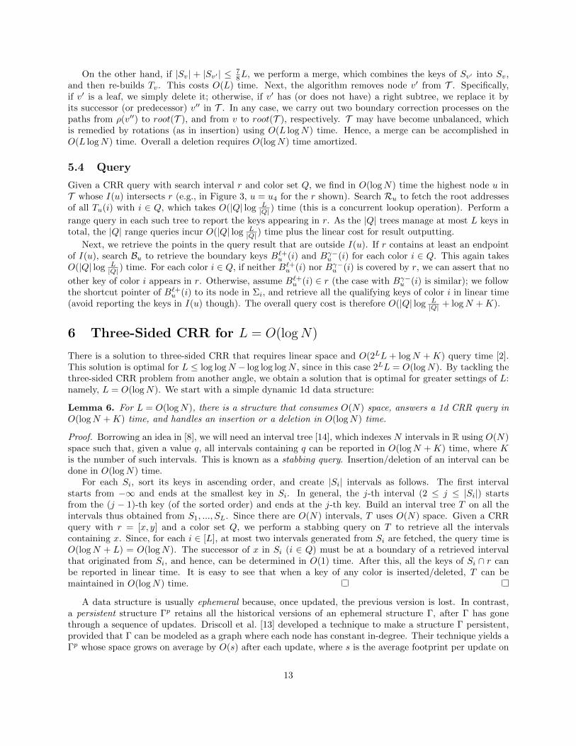
RI(u1) I(u2) I(u3) I(u4) I(u5) I(u6)
u1
u2
u3
u4
u5
u6
r
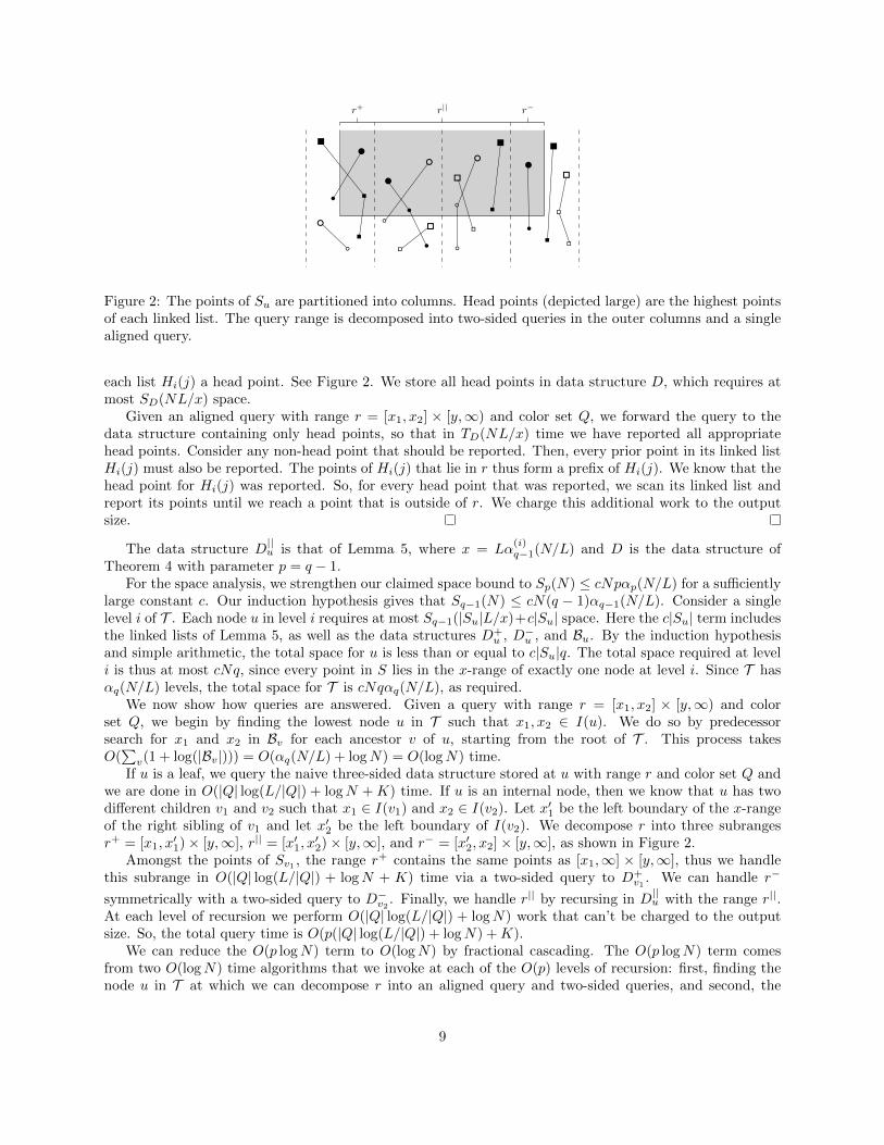
Figure 3: A BST with fat nodes
of Θ(L) consecutive keys4 in S. T is created on the obvious total order of all the nodes. The ordering alsoassociates each node u with a range I(u) ⊆ R in the form of [α, β), where α is the smallest key in u, and βis the smallest key in the node succeeding u (if such a node does not exist, β =∞). See Figure 3. For eachnode u in T , we organize the keys of Su in L BSTs Tu(1), ..., Tu(L), where Tu(i) manages the color-i keys inSu. Index the root addresses of Tu(1), ..., Tu(L) in a BST Ru.
Denote by Du the set of keys stored in the subtree of u. Let `(u) (γ(u)) be the left (right) child of nodeu, or ∅ if the child does not exist. Define 4L boundary keys as follows:
• For each i ∈ [L], B`−u (i) (B`+u (i)) is the minimum (maximum) key of color i in D`(u). If D`(u) has no
key of this color, B`−u (i) = B`+u (i) = ∅.
• Bγ−u (i) and Bγ+u (i) are defined analogously with respect to Dγ(u).
The 4L boundary keys can be divided into L boundary groups, where the i-th group is a 4-tuple(B`−u (i), B`+u (i), Bγ−u (i), Bγ+u (i)). These groups are indexed by their colors with a BST Bu (i.e., each nodeof Bu stores a boundary group). For update efficiency, we keep some down pointers. Specifically for eachi ∈ [L], the color-i node of Bu stores two down pointers referencing the color-i nodes in B`(u) and Bγ(u),respectively. If `(u) (γ(u)) = ∅, the down pointer to B`(u) (Bγ(u)) is nil . Finally, the keys of each Si areindexed with a BST Σi, called an exclusive BST. Each key k in T (including boundary keys) is associatedwith a shortcut pointer, referencing node k in the corresponding exclusive BST.
All the exclusive BSTs occupy totally O(N) space. At each node u of T , all the secondary structuresrequire O(|Su|+L) space. Hence, the overall size of our structure is
∑uO(|Su|+L) = O(N), noticing that
T has O(N/L) nodes.
5.2 Insertion
Let all the BSTs be implemented as AVL-trees. For any non-root node u, denote its parent as ρ(u). Supposethat we need to insert a key k of color c ∈ [L]. First, k is added to Σc in O(logN) time. Then, we identifythe node v in T such that k ∈ I(v), which costs O(log N
L ) time, i.e., same as the height of T . For eachnode u on the path from root(T ) to v, update two of its boundary keys of color c. To illustrate, assumethat v is in the left (the case of right is symmetric) subtree of u; we adjust the boundary key B`−u (c) tominB`−u (c), k, and B`+u (c) to maxB`+u (c), k. These boundary keys can be found efficiently using thedown pointers. First, the (color-c) boundary group of root(T ) is retrieved by searching Broot(T ) in O(logL)time. In general, having found a boundary group at a parent node ρ(u), we follow a down pointer of thegroup to obtain the boundary group of the same color at u in O(1) time. Hence, the entire process takesO(logL+ log N
L ) = O(logN) time.At v, k is inserted into Tv(c) in O(logL) time. If |Sv| is now at most L, the insertion is completed.
Otherwise, v overflows, and needs to be split into v1 and v2. For this purpose, we sort all the keys in Sv inO(L logL) time, divide the sorted list in two equal halves, and take the first (second) half as Sv1 (Sv2). Then,the secondary BSTs Tv1(1), ..., Tv1(L),Rv1 and Tv2(1), ..., Tv2(L),Rv2 can be built in O(L) time. Nodes v1
4The only exception is when T has only one node u, in which case |Su| can be anywhere from 1 to L.
11
u1
u2
u3
u4
u5⇒
u1 u4
u3
u2
u5u1
u2
u3
u4
u5
⇒
u6
u7
u1
u2
u3
u4
u6
u5u7
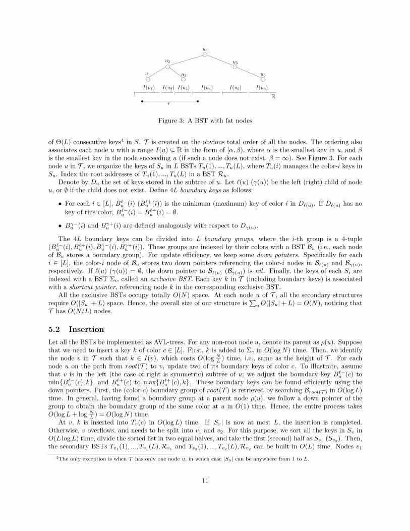
(a) Single rotation (b) Double rotation
Figure 4: Rotations in an AVL-tree
and v2 need to be incorporated in T . For this purpose, we first replace v with v1 in T and set Bv1 directlyto Bv, which takes O(1) time. Then, v2 is inserted in the right subtree of v (now v1) as in the BST. Whenthis is done, v2 is a leaf of T , and some boundary keys of the nodes on the path from ρ(v2) to v1 may nowbe incorrect. A boundary correction is carried out to fix them in a bottom-up manner:
• Suppose, without loss of generality, that v2 is the left child of ρ(v2). For each i ∈ [L], set B`−ρ(v2)(i) =
mink(Sv2 , i) and B`+ρ(v2)(i) = maxk(Sv2 , i), where mink(X, i) and maxk(X, i) return the smallest and
largest color-i key in a set X of keys, respectively. We then build Bρ(v2) in O(L) time.
• In general, having fixed node u, the correction process works at ρ(u) as follows, again assuming u tobe the left child of ρ(u). For each i ∈ [L], we set:
B`−ρ(u)(i) = minB`−u (i),mink(Su, i), Bγ−u (i)
B`+ρ(u)(i) = maxB`+u (i),maxk(Su, i), Bγ+u (i).
The correction spends O(L) time per level, noticing that mink(Su, i) and maxk(Su, i) of all i ∈ [L] can beretrieved in O(
∑i log |Tu(i)|) = O(L) time, where |Tu(i)| is the number of nodes in Tu(i).
If T is unbalanced, we perform a single- or double-rotation as in the AVL-tree. Each rotation modifiesO(1) pointers, as illustrated by bold lines in Figure 4. In our context, a rotation is followed by boundarycorrection. Specifically, in Figure 4a, we launch a correction process to fix the boundary keys from u4 tou2 whereas, in Figure 4b, two processes are invoked to fix the paths from u2 to u4 and from u6 to u4,respectively. Since only two levels are corrected, all processes take O(L) time. The above description hasnot included the maintenance of down and shortcut pointers, but this can be easily taken care of at no extracost asymptotically.
If no overflow happens, an insertion terminates in O(logN) time. Otherwise, the cost is O(L logN).However, as a node u overflows only after Ω(L) keys have been newly inserted in Su, each update is chargedO(logN) time.
5.3 Deletion
Suppose that we are deleting a key k of color c ∈ [L]. The deletion algorithm starts by removing k from Σcin O(logN) time. Then, we find in O(log N
L ) time the node v in T such that k ∈ Iv, and remove k fromTv(c) in O(logL) time. As k may be serving as a boundary key at the nodes on the path from v to root(T ),we fix their boundary keys in a way similar to a boundary correction process, except that here we focus ononly a unique color c. Using down pointers, all the boundary keys to be fixed can be identified in O(logN)time.
If now Sv has at least L/4 keys, the deletion is completed. Otherwise, v underflows, which is treated bya share or merge (reminiscent of underflow-handing in a B-tree). Specifically, the algorithm first identifiesin O(log N
L ) time the successor v′ of v in T . If |Sv| + |Sv′ | > 78L, we perform a share, which re-distributes
the keys in Sv and Sv′ evenly. This, in turn, necessitates rebuilding Tv and Tv′ , and a boundary correctionprocess from either v or v′ (whichever is lower) to root(T ). The total time required is O(L logL).
12
On the other hand, if |Sv| + |Sv′ | ≤ 78L, we perform a merge, which combines the keys of Sv′ into Sv,
and then re-builds Tv. This costs O(L) time. Next, the algorithm removes node v′ from T . Specifically,if v′ is a leaf, we simply delete it; otherwise, if v′ has (or does not have) a right subtree, we replace it byits successor (or predecessor) v′′ in T . In any case, we carry out two boundary correction processes on thepaths from ρ(v′′) to root(T ), and from v to root(T ), respectively. T may have become unbalanced, whichis remedied by rotations (as in insertion) using O(L logN) time. Hence, a merge can be accomplished inO(L logN) time. Overall a deletion requires O(logN) time amortized.
5.4 Query
Given a CRR query with search interval r and color set Q, we find in O(logN) time the highest node u inT whose I(u) intersects r (e.g., in Figure 3, u = u4 for the r shown). Search Ru to fetch the root addressesof all Tu(i) with i ∈ Q, which takes O(|Q| log L
|Q| ) time (this is a concurrent lookup operation). Perform a
range query in each such tree to report the keys appearing in r. As the |Q| trees manage at most L keys intotal, the |Q| range queries incur O(|Q| log L
|Q| ) time plus the linear cost for result outputting.
Next, we retrieve the points in the query result that are outside I(u). If r contains at least an endpointof I(u), search Bu to retrieve the boundary keys B`+u (i) and Bγ−u (i) for each color i ∈ Q. This again takesO(|Q| log L
|Q| ) time. For each color i ∈ Q, if neither B`+u (i) nor Bγ−u (i) is covered by r, we can assert that no
other key of color i appears in r. Otherwise, assume B`+u (i) ∈ r (the case with Bγ−u (i) is similar); we followthe shortcut pointer of B`+u (i) to its node in Σi, and retrieve all the qualifying keys of color i in linear time(avoid reporting the keys in I(u) though). The overall query cost is therefore O(|Q| log L
|Q| + logN +K).
6 Three-Sided CRR for L = O(logN)
There is a solution to three-sided CRR that requires linear space and O(2LL + logN + K) query time [2].This solution is optimal for L ≤ log logN − log log logN , since in this case 2LL = O(logN). By tackling thethree-sided CRR problem from another angle, we obtain a solution that is optimal for greater settings of L:namely, L = O(logN). We start with a simple dynamic 1d data structure:
Lemma 6. For L = O(logN), there is a structure that consumes O(N) space, answers a 1d CRR query inO(logN +K) time, and handles an insertion or a deletion in O(logN) time.
Proof. Borrowing an idea in [8], we will need an interval tree [14], which indexes N intervals in R using O(N)space such that, given a value q, all intervals containing q can be reported in O(logN +K) time, where Kis the number of such intervals. This is known as a stabbing query. Insertion/deletion of an interval can bedone in O(logN) time.
For each Si, sort its keys in ascending order, and create |Si| intervals as follows. The first intervalstarts from −∞ and ends at the smallest key in Si. In general, the j-th interval (2 ≤ j ≤ |Si|) startsfrom the (j − 1)-th key (of the sorted order) and ends at the j-th key. Build an interval tree T on all theintervals thus obtained from S1, ..., SL. Since there are O(N) intervals, T uses O(N) space. Given a CRRquery with r = [x, y] and a color set Q, we perform a stabbing query on T to retrieve all the intervalscontaining x. Since, for each i ∈ [L], at most two intervals generated from Si are fetched, the query time isO(logN + L) = O(logN). The successor of x in Si (i ∈ Q) must be at a boundary of a retrieved intervalthat originated from Si, and hence, can be determined in O(1) time. After this, all the keys of Si ∩ r canbe reported in linear time. It is easy to see that when a key of any color is inserted/deleted, T can bemaintained in O(logN) time.
A data structure is usually ephemeral because, once updated, the previous version is lost. In contrast,a persistent structure Γp retains all the historical versions of an ephemeral structure Γ, after Γ has gonethrough a sequence of updates. Driscoll et al. [13] developed a technique to make a structure Γ persistent,provided that Γ can be modeled as a graph where each node has constant in-degree. Their technique yields aΓp whose space grows on average by O(s) after each update, where s is the average footprint per update on
13

Γ. Γp can be constructed in the same time as performing all the corresponding updates on Γ. Furthermore,Γp inherits the query complexity of Γ, with only an O(logN) additive cost to identify the correct version.
In general, three-sided range searching can be supported by the persistent counterpart of a structuredesigned for 1d range searching. Imagine that we move a horizontal sweeping line downwards, starting fromthe top of R2. Whenever the line hits a point p ∈ S, insert the x-coordinate of p in a 1d-CRR structure Γ.Denote by Γ(λ) the version of Γ when the sweeping line intersects the y-axis at λ. Given a three-sided querywith r = [x1, x2]× [y,∞), we answer it by performing a 1d-CRR query with r = [x1, x2] on Γ(y). Based onthis idea, we prove:
Lemma 7. For L = O(logN), there is a linear-space structure that answers a three-sided CRR query inO(logN +K) time, and can be built in O(N logN) time.
Proof. Our structure in Lemma 6 is indeed a graph where nodes have constant in-degree. As shown in [6],each insertion in the interval tree takes O(logN) time, and leaves only O(1) footprint on average5.
7 Open Problems
It remains open whether three-sided CRR can be solved in linear space and O(|Q| log(L/|Q|) + logN +K)query time. In the RAM model, 1d CRR can be solved in linear space and O(|Q| + K) query time, sincetraditional 1d range searching can be solved in linear space and O(1 +K) query time [5]. However, the samecannot be said for the concurrent predecessor search problem, since traditional predecessor search in theRAM model using polynomial space requires super-constant query time [18]. It is open whether concurrentpredecessor search can be solved in linear space and O(Tpred + |Q|+K) query time, where Tpred is the costof traditional predecessor search in the RAM model.
Another problem for which a concurrent variant is interesting is point location. In concurrent pointlocation we must preprocess L subdivisions of the plane S1, S2, . . . , SL. Given a query point q and a setof colors Q ⊆ [L], we must locate q in Si for i ∈ Q. This concurrent point location problem is closelyrelated to a 2d generalization of fractional cascading studied by Chazelle and Liu [11]. Chazelle and Liushow that no efficient bounds can be achieved for the 2d generalization of fractional cascading without usingat least quadratic space. However, the hard instance in their lower bound uses non-orthogonal subdivisionsof the plane. In the special case of concurrent orthogonal point location, there is a simple linear-space datastructure that requires O(L+ logN +K) query time: decompose the subdivisions into rectangles and storethese rectangles in the rectangle-stabbing data structure of Chazelle [8]. It is open whether the L term inthis query time can be reduced to O(|Q| log(L/|Q|)) as in our CRR data structures.
References
[1] P. Afshani. Improved pointer machine and I/O lower bounds for simplex range reporting and relatedproblems. In Symposium on Computational Geometry (SoCG), pages 339–346, 2012.
[2] P. Afshani, L. Arge, and K. D. Larsen. Orthogonal range reporting in three and higher dimensions. InProceedings of Annual IEEE Symposium on Foundations of Computer Science (FOCS), pages 149–158,2009.
[3] P. Afshani, L. Arge, and K. D. Larsen. Orthogonal range reporting: query lower bounds, optimalstructures in 3-d, and higher-dimensional improvements. In Symposium on Computational Geometry(SoCG), pages 240–246, 2010.
[4] P. K. Agarwal, S. Govindarajan, and S. Muthukrishnan. Range searching in categorical data: Coloredrange searching on grid. In Proceedings of European Symposium on Algorithms (ESA), pages 17–28,2002.
5The result of [6] holds in the offline setting, i.e., all the insertions are known in advance. This is sufficient for our purposehere.
14
[5] S. Alstrup, G. S. Brodal, and T. Rauhe. Optimal static range reporting in one dimension. In Proceedingsof ACM Symposium on Theory of Computing (STOC), pages 476–482, 2001.
[6] A. Boroujerdi and B. M. E. Moret. Persistency in computational geometry. In Proceedings of theCanadian Conference on Computational Geometry (CCCG), pages 241–246, 1995.
[7] B. Chazelle. On the convex layers of a planar set. IEEE Transactions on Information Theory, 31(4):509–517, 1985.
[8] B. Chazelle. Filtering search: A new approach to query-answering. SIAM Journal of Computing,15(3):703–724, 1986.
[9] B. Chazelle and L. J. Guibas. Fractional cascading: I. a data structuring technique. Algorithmica,1(2):133–162, 1986.
[10] B. Chazelle and L. J. Guibas. Fractional cascading: II. applications. Algorithmica, 1(2):163–191, 1986.
[11] B. Chazelle and D. Liu. Lower bounds for intersection searching and fractional cascading in higherdimension. Journal of Computer and System Sciences (JCSS), 68(2):269–284, 2004.
[12] T. H. Cormen, C. E. Leiserson, R. L. Rivest, and C. Stein. Introduction to Algorithms, Second Edition.The MIT Press, 2001.
[13] J. R. Driscoll, N. Sarnak, D. D. Sleator, and R. E. Tarjan. Making data structures persistent. Journalof Computer and System Sciences (JCSS), 38(1):86–124, 1989.
[14] H. Edelsbrunner. A new approach to rectangle intersections, part I. International Journal of ComputerMathematics, 13:209–219, 1983.
[15] E. M. McCreight. Priority search trees. SIAM Journal of Computing, 14(2):257–276, 1985.
[16] K. Mehlhorn and S. Naher. Dynamic fractional cascading. Algorithmica, 5(2):215–241, 1990.
[17] M. H. Overmars. Efficient data structures for range searching on a grid. J. Algorithms, 9(2):254–275,1988.
[18] M. Patrascu and M. Thorup. Time-space trade-offs for predecessor search. In Proceedings of ACMSymposium on Theory of Computing (STOC), pages 232–240, 2006.
15