Embed Size (px)
Citation preview
COMS 4995 Lecture 2:Multilayer Perceptrons & Backpropagation
Richard Zemel
Richard Zemel COMS 4995 Lecture 2: Multilayer Perceptrons & Backpropagation 1 / 44
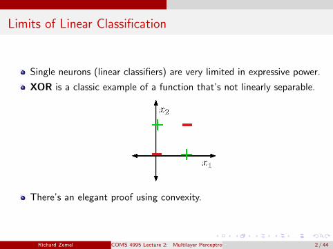
Limits of Linear Classification
Single neurons (linear classifiers) are very limited in expressive power.
XOR is a classic example of a function that’s not linearly separable.
There’s an elegant proof using convexity.
Richard Zemel COMS 4995 Lecture 2: Multilayer Perceptrons & Backpropagation 2 / 44
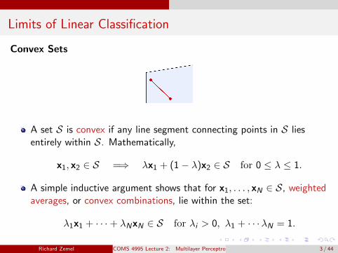
Limits of Linear Classification
Convex Sets
A set S is convex if any line segment connecting points in S liesentirely within S. Mathematically,
x1, x2 ∈ S =⇒ λx1 + (1− λ)x2 ∈ S for 0 ≤ λ ≤ 1.
A simple inductive argument shows that for x1, . . . , xN ∈ S, weightedaverages, or convex combinations, lie within the set:
λ1x1 + · · ·+ λNxN ∈ S for λi > 0, λ1 + · · ·λN = 1.
Richard Zemel COMS 4995 Lecture 2: Multilayer Perceptrons & Backpropagation 3 / 44
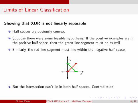
Limits of Linear Classification
Showing that XOR is not linearly separable
Half-spaces are obviously convex.
Suppose there were some feasible hypothesis. If the positive examples are inthe positive half-space, then the green line segment must be as well.
Similarly, the red line segment must line within the negative half-space.
But the intersection can’t lie in both half-spaces. Contradiction!
Richard Zemel COMS 4995 Lecture 2: Multilayer Perceptrons & Backpropagation 4 / 44
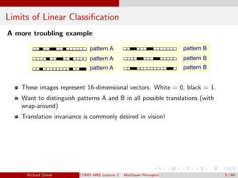
Limits of Linear Classification
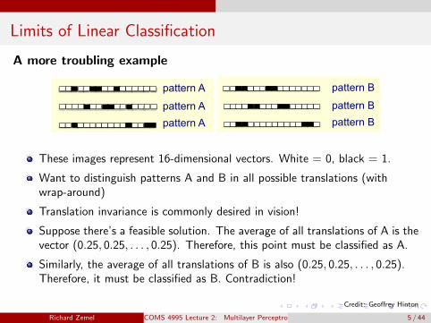
A more troubling example
Discriminating simple patterns under translation with wrap-around
• Suppose we just use pixels as the features.
• Can a binary threshold unit discriminate between different patterns that have the same number of on pixels? – Not if the patterns can
translate with wrap-around!
pattern A
pattern A
pattern A
pattern B
pattern B
pattern B
These images represent 16-dimensional vectors. White = 0, black = 1.
Want to distinguish patterns A and B in all possible translations (withwrap-around)
Translation invariance is commonly desired in vision!
Suppose there’s a feasible solution. The average of all translations of A is thevector (0.25, 0.25, . . . , 0.25). Therefore, this point must be classified as A.
Similarly, the average of all translations of B is also (0.25, 0.25, . . . , 0.25).Therefore, it must be classified as B. Contradiction!
Credit: Geoffrey Hinton
Richard Zemel COMS 4995 Lecture 2: Multilayer Perceptrons & Backpropagation 5 / 44
Limits of Linear Classification
A more troubling example
Discriminating simple patterns under translation with wrap-around
• Suppose we just use pixels as the features.
• Can a binary threshold unit discriminate between different patterns that have the same number of on pixels? – Not if the patterns can
translate with wrap-around!
pattern A
pattern A
pattern A
pattern B
pattern B
pattern B
Discriminating simple patterns under translation with wrap-around
• Suppose we just use pixels as the features.
• Can a binary threshold unit discriminate between different patterns that have the same number of on pixels? – Not if the patterns can
translate with wrap-around!
pattern A
pattern A
pattern A
pattern B
pattern B
pattern B
These images represent 16-dimensional vectors. White = 0, black = 1.
Want to distinguish patterns A and B in all possible translations (withwrap-around)
Translation invariance is commonly desired in vision!
Suppose there’s a feasible solution. The average of all translations of A is thevector (0.25, 0.25, . . . , 0.25). Therefore, this point must be classified as A.
Similarly, the average of all translations of B is also (0.25, 0.25, . . . , 0.25).Therefore, it must be classified as B. Contradiction!
Credit: Geoffrey Hinton
Richard Zemel COMS 4995 Lecture 2: Multilayer Perceptrons & Backpropagation 5 / 44
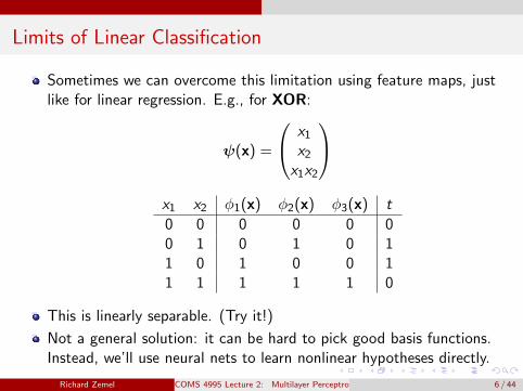
Limits of Linear Classification
Sometimes we can overcome this limitation using feature maps, justlike for linear regression. E.g., for XOR:
ψ(x) =
x1
x2
x1x2
x1 x2 φ1(x) φ2(x) φ3(x) t
0 0 0 0 0 00 1 0 1 0 11 0 1 0 0 11 1 1 1 1 0
This is linearly separable. (Try it!)
Not a general solution: it can be hard to pick good basis functions.Instead, we’ll use neural nets to learn nonlinear hypotheses directly.
Richard Zemel COMS 4995 Lecture 2: Multilayer Perceptrons & Backpropagation 6 / 44

Multilayer Perceptrons
We can connect lots ofunits together into adirected acyclic graph.
This gives a feed-forwardneural network. That’sin contrast to recurrentneural networks, whichcan have cycles. (We’lltalk about those later.)
Typically, units aregrouped together intolayers.
Richard Zemel COMS 4995 Lecture 2: Multilayer Perceptrons & Backpropagation 7 / 44

Multilayer Perceptrons
Each layer connects N input units to M output units.
In the simplest case, all input units are connected to all output units. We call thisa fully connected layer. We’ll consider other layer types later.
Note: the inputs and outputs for a layer are distinct from the inputs and outputsto the network.
Recall from softmax regression: this means weneed an M × N weight matrix.
The output units are a function of the inputunits:
y = f (x) = φ (Wx + b)
A multilayer network consisting of fullyconnected layers is called a multilayerperceptron. Despite the name, it has nothingto do with perceptrons!
Richard Zemel COMS 4995 Lecture 2: Multilayer Perceptrons & Backpropagation 8 / 44
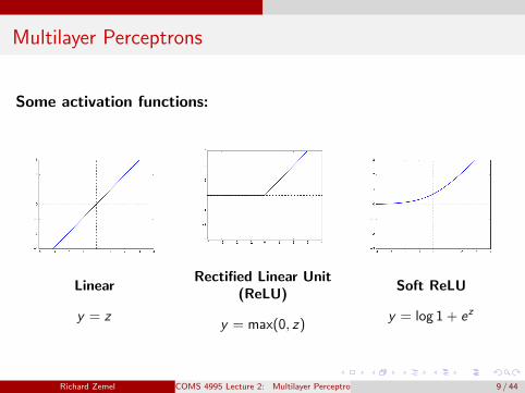
Multilayer Perceptrons
Some activation functions:
Linear
y = z
Rectified Linear Unit(ReLU)
y = max(0, z)
Soft ReLU
y = log 1 + ez
Richard Zemel COMS 4995 Lecture 2: Multilayer Perceptrons & Backpropagation 9 / 44
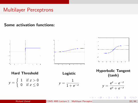
Multilayer Perceptrons
Some activation functions:
Hard Threshold
y =
{1 if z > 00 if z ≤ 0
Logistic
y =1
1 + e−z
Hyperbolic Tangent(tanh)
y =ez − e−z
ez + e−z
Richard Zemel COMS 4995 Lecture 2: Multilayer Perceptrons & Backpropagation 10 / 44
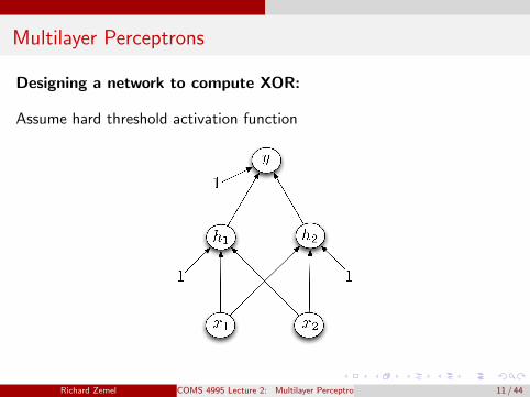
Multilayer Perceptrons
Designing a network to compute XOR:
Assume hard threshold activation function
Richard Zemel COMS 4995 Lecture 2: Multilayer Perceptrons & Backpropagation 11 / 44
Multilayer Perceptrons
Richard Zemel COMS 4995 Lecture 2: Multilayer Perceptrons & Backpropagation 12 / 44
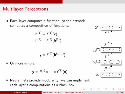
Multilayer Perceptrons
Each layer computes a function, so the networkcomputes a composition of functions:
h(1) = f (1)(x)
h(2) = f (2)(h(1))
...
y = f (L)(h(L−1))
Or more simply:
y = f (L) ◦ · · · ◦ f (1)(x).
Neural nets provide modularity: we can implementeach layer’s computations as a black box.
Richard Zemel COMS 4995 Lecture 2: Multilayer Perceptrons & Backpropagation 13 / 44

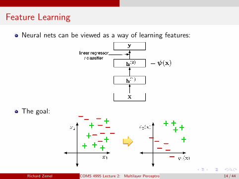
Feature Learning
Neural nets can be viewed as a way of learning features:
The goal:
Richard Zemel COMS 4995 Lecture 2: Multilayer Perceptrons & Backpropagation 14 / 44
Feature Learning
Neural nets can be viewed as a way of learning features:
The goal:
Richard Zemel COMS 4995 Lecture 2: Multilayer Perceptrons & Backpropagation 14 / 44
Feature Learning
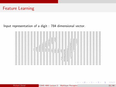
Input representation of a digit : 784 dimensional vector.
Richard Zemel COMS 4995 Lecture 2: Multilayer Perceptrons & Backpropagation 15 / 44
Feature Learning
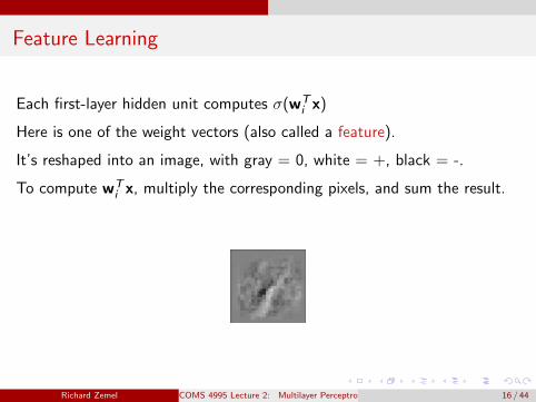
Each first-layer hidden unit computes σ(wTi x)
Here is one of the weight vectors (also called a feature).
It’s reshaped into an image, with gray = 0, white = +, black = -.
To compute wTi x, multiply the corresponding pixels, and sum the result.
Richard Zemel COMS 4995 Lecture 2: Multilayer Perceptrons & Backpropagation 16 / 44
Feature Learning
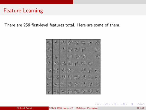
There are 256 first-level features total. Here are some of them.
Richard Zemel COMS 4995 Lecture 2: Multilayer Perceptrons & Backpropagation 17 / 44
Expressive Power
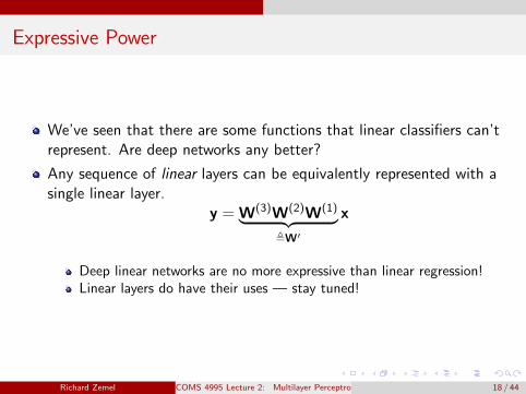
We’ve seen that there are some functions that linear classifiers can’trepresent. Are deep networks any better?
Any sequence of linear layers can be equivalently represented with asingle linear layer.
y = W(3)W(2)W(1)︸ ︷︷ ︸,W′
x
Deep linear networks are no more expressive than linear regression!Linear layers do have their uses — stay tuned!
Richard Zemel COMS 4995 Lecture 2: Multilayer Perceptrons & Backpropagation 18 / 44
Expressive Power
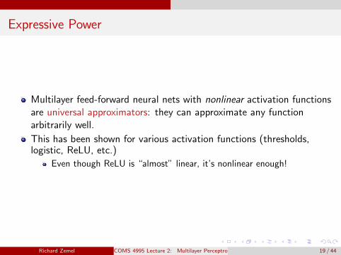
Multilayer feed-forward neural nets with nonlinear activation functionsare universal approximators: they can approximate any functionarbitrarily well.
This has been shown for various activation functions (thresholds,logistic, ReLU, etc.)
Even though ReLU is “almost” linear, it’s nonlinear enough!
Richard Zemel COMS 4995 Lecture 2: Multilayer Perceptrons & Backpropagation 19 / 44
Expressive Power
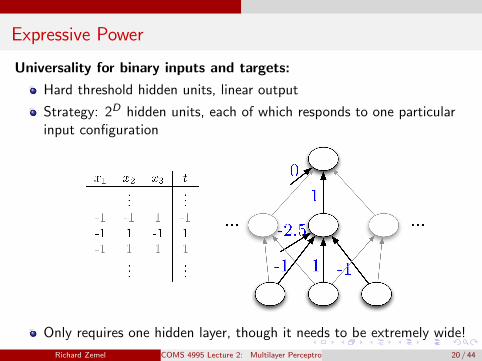
Universality for binary inputs and targets:
Hard threshold hidden units, linear output
Strategy: 2D hidden units, each of which responds to one particularinput configuration
Only requires one hidden layer, though it needs to be extremely wide!
Richard Zemel COMS 4995 Lecture 2: Multilayer Perceptrons & Backpropagation 20 / 44
Expressive Power
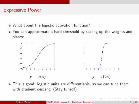
What about the logistic activation function?
You can approximate a hard threshold by scaling up the weights andbiases:
y = σ(x) y = σ(5x)
This is good: logistic units are differentiable, so we can tune themwith gradient descent. (Stay tuned!)
Richard Zemel COMS 4995 Lecture 2: Multilayer Perceptrons & Backpropagation 21 / 44

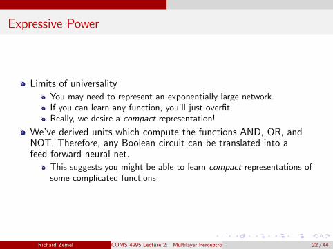
Expressive Power
Limits of universality
You may need to represent an exponentially large network.If you can learn any function, you’ll just overfit.Really, we desire a compact representation!
We’ve derived units which compute the functions AND, OR, andNOT. Therefore, any Boolean circuit can be translated into afeed-forward neural net.
This suggests you might be able to learn compact representations ofsome complicated functions
Richard Zemel COMS 4995 Lecture 2: Multilayer Perceptrons & Backpropagation 22 / 44
Overview
We’ve seen that multilayer neural networks are powerful. But how canwe actually learn them?
Backpropagation is the central algorithm in this course.
It’s is an algorithm for computing gradients.Really it’s an instance of reverse mode automatic differentiation, whichis much more broadly applicable than just neural nets.
This is “just” a clever and efficient use of the Chain Rule for derivatives.We’ll see how to implement an automatic differentiation system soon.
Richard Zemel COMS 4995 Lecture 2: Multilayer Perceptrons & Backpropagation 23 / 44
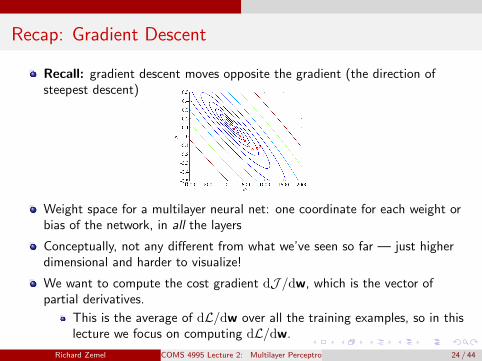
Recap: Gradient Descent
Recall: gradient descent moves opposite the gradient (the direction ofsteepest descent)
Weight space for a multilayer neural net: one coordinate for each weight orbias of the network, in all the layers
Conceptually, not any different from what we’ve seen so far — just higherdimensional and harder to visualize!
We want to compute the cost gradient dJ /dw, which is the vector ofpartial derivatives.
This is the average of dL/dw over all the training examples, so in thislecture we focus on computing dL/dw.
Richard Zemel COMS 4995 Lecture 2: Multilayer Perceptrons & Backpropagation 24 / 44

Univariate Chain Rule
We’ve already been using the univariate Chain Rule.
Recall: if f (x) and x(t) are univariate functions, then
d
dtf (x(t)) =
df
dx
dx
dt.
Richard Zemel COMS 4995 Lecture 2: Multilayer Perceptrons & Backpropagation 25 / 44
Univariate Chain Rule
Recall: Univariate logistic least squares model
z = wx + b
y = σ(z)
L =1
2(y − t)2
Let’s compute the loss derivatives.
Richard Zemel COMS 4995 Lecture 2: Multilayer Perceptrons & Backpropagation 26 / 44
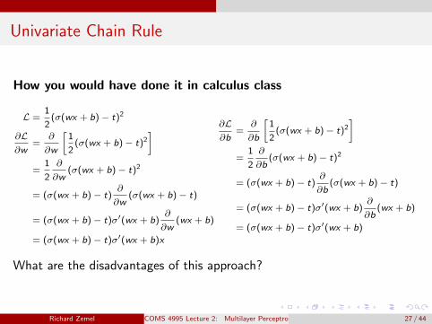
Univariate Chain Rule
How you would have done it in calculus class
L =1
2(σ(wx + b)− t)2
∂L∂w
=∂
∂w
[1
2(σ(wx + b)− t)2
]=
1
2
∂
∂w(σ(wx + b)− t)2
= (σ(wx + b)− t)∂
∂w(σ(wx + b)− t)
= (σ(wx + b)− t)σ′(wx + b)∂
∂w(wx + b)
= (σ(wx + b)− t)σ′(wx + b)x
∂L∂b
=∂
∂b
[1
2(σ(wx + b)− t)2
]=
1
2
∂
∂b(σ(wx + b)− t)2
= (σ(wx + b)− t)∂
∂b(σ(wx + b)− t)
= (σ(wx + b)− t)σ′(wx + b)∂
∂b(wx + b)
= (σ(wx + b)− t)σ′(wx + b)
What are the disadvantages of this approach?
Richard Zemel COMS 4995 Lecture 2: Multilayer Perceptrons & Backpropagation 27 / 44
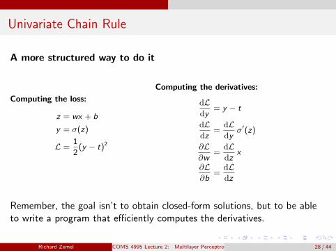
Univariate Chain Rule
A more structured way to do it
Computing the loss:
z = wx + b
y = σ(z)
L =1
2(y − t)2
Computing the derivatives:
dLdy
= y − t
dLdz
=dLdy
σ′(z)
∂L∂w
=dLdz
x
∂L∂b
=dLdz
Remember, the goal isn’t to obtain closed-form solutions, but to be ableto write a program that efficiently computes the derivatives.
Richard Zemel COMS 4995 Lecture 2: Multilayer Perceptrons & Backpropagation 28 / 44
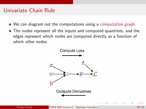
Univariate Chain Rule
We can diagram out the computations using a computation graph.
The nodes represent all the inputs and computed quantities, and theedges represent which nodes are computed directly as a function ofwhich other nodes.
Richard Zemel COMS 4995 Lecture 2: Multilayer Perceptrons & Backpropagation 29 / 44
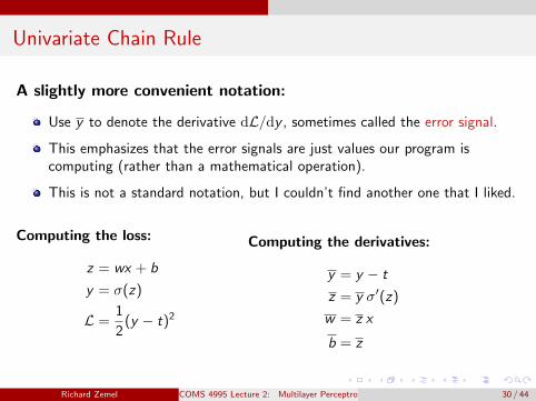
Univariate Chain Rule
A slightly more convenient notation:
Use y to denote the derivative dL/dy , sometimes called the error signal.
This emphasizes that the error signals are just values our program iscomputing (rather than a mathematical operation).
This is not a standard notation, but I couldn’t find another one that I liked.
Computing the loss:
z = wx + b
y = σ(z)
L =1
2(y − t)2
Computing the derivatives:
y = y − t
z = y σ′(z)
w = z x
b = z
Richard Zemel COMS 4995 Lecture 2: Multilayer Perceptrons & Backpropagation 30 / 44
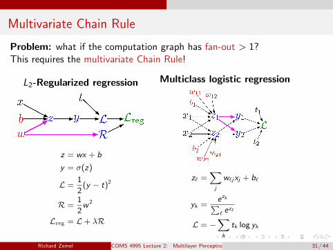
Multivariate Chain Rule
Problem: what if the computation graph has fan-out > 1?This requires the multivariate Chain Rule!
L2-Regularized regression
z = wx + b
y = σ(z)
L =1
2(y − t)2
R =1
2w 2
Lreg = L+ λR
Multiclass logistic regression
z` =∑j
w`jxj + b`
yk =ezk∑` e
z`
L = −∑k
tk log yk
Richard Zemel COMS 4995 Lecture 2: Multilayer Perceptrons & Backpropagation 31 / 44
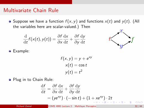
Multivariate Chain Rule
Suppose we have a function f (x , y) and functions x(t) and y(t). (Allthe variables here are scalar-valued.) Then
d
dtf (x(t), y(t)) =
∂f
∂x
dx
dt+∂f
∂y
dy
dt
Example:
f (x , y) = y + exy
x(t) = cos t
y(t) = t2
Plug in to Chain Rule:
df
dt=∂f
∂x
dx
dt+∂f
∂y
dy
dt
= (yexy ) · (− sin t) + (1 + xexy ) · 2t
Richard Zemel COMS 4995 Lecture 2: Multilayer Perceptrons & Backpropagation 32 / 44
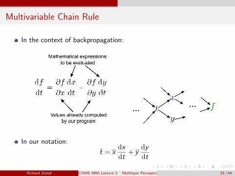
Multivariable Chain Rule
In the context of backpropagation:
In our notation:
t = xdx
dt+ y
dy
dt
Richard Zemel COMS 4995 Lecture 2: Multilayer Perceptrons & Backpropagation 33 / 44
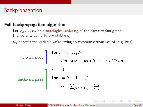
Backpropagation
Full backpropagation algorithm:
Let v1, . . . , vN be a topological ordering of the computation graph(i.e. parents come before children.)
vN denotes the variable we’re trying to compute derivatives of (e.g. loss).
Richard Zemel COMS 4995 Lecture 2: Multilayer Perceptrons & Backpropagation 34 / 44

Backpropagation
Example: univariate logistic least squares regression
Forward pass:
z = wx + b
y = σ(z)
L =1
2(y − t)2
R =1
2w 2
Lreg = L+ λR
Backward pass:
Lreg = 1
R = LregdLreg
dR= Lreg λ
L = LregdLreg
dL= Lreg
y = L dLdy
= L (y − t)
z = ydy
dz
= y σ′(z)
w= z∂z
∂w+RdR
dw
= z x +Rw
b = z∂z
∂b
= z
Richard Zemel COMS 4995 Lecture 2: Multilayer Perceptrons & Backpropagation 35 / 44
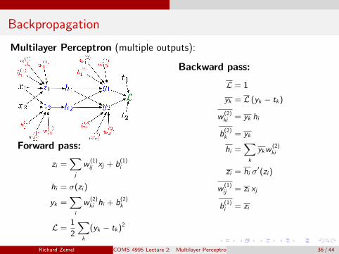
Backpropagation
Multilayer Perceptron (multiple outputs):
Forward pass:
zi =∑j
w(1)ij xj + b
(1)i
hi = σ(zi )
yk =∑i
w(2)ki hi + b
(2)k
L =1
2
∑k
(yk − tk)2
Backward pass:
L = 1
yk = L (yk − tk)
w(2)ki = yk hi
b(2)k = yk
hi =∑k
ykw(2)ki
zi = hi σ′(zi )
w(1)ij = zi xj
b(1)i = zi
Richard Zemel COMS 4995 Lecture 2: Multilayer Perceptrons & Backpropagation 36 / 44

Vector Form
Computation graphs showing individual units are cumbersome.
As you might have guessed, we typically draw graphs over thevectorized variables.
We pass messages back analogous to the ones for scalar-valued nodes.
Richard Zemel COMS 4995 Lecture 2: Multilayer Perceptrons & Backpropagation 37 / 44
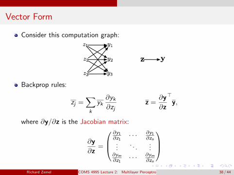
Vector Form
Consider this computation graph:
Backprop rules:
zj =∑k
yk∂yk∂zj
z =∂y
∂z
>y,
where ∂y/∂z is the Jacobian matrix:
∂y
∂z=
∂y1∂z1
· · · ∂y1∂zn
.... . .
...∂ym∂z1
· · · ∂ym∂zn
Richard Zemel COMS 4995 Lecture 2: Multilayer Perceptrons & Backpropagation 38 / 44

Vector Form
Examples
Matrix-vector product
z = Wx∂z
∂x= W x = W>z
Elementwise operations
y = exp(z)∂y
∂z=
exp(z1) 0. . .
0 exp(zD)
z = exp(z) ◦ y
Note: we never explicitly construct the Jacobian. It’s usually simplerand more efficient to compute the VJP directly.
Richard Zemel COMS 4995 Lecture 2: Multilayer Perceptrons & Backpropagation 39 / 44
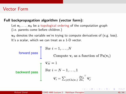
Vector Form
Full backpropagation algorithm (vector form):
Let v1, . . . , vN be a topological ordering of the computation graph(i.e. parents come before children.)
vN denotes the variable we’re trying to compute derivatives of (e.g. loss).
It’s a scalar, which we can treat as a 1-D vector.
Richard Zemel COMS 4995 Lecture 2: Multilayer Perceptrons & Backpropagation 40 / 44
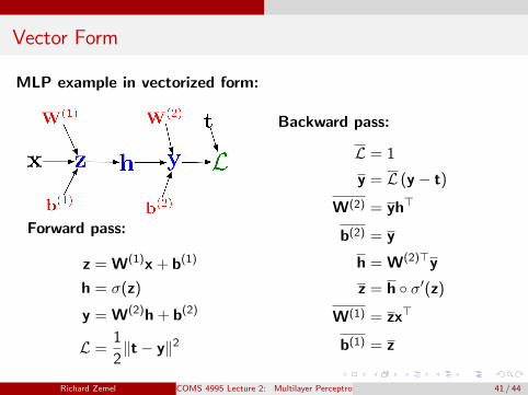
Vector Form
MLP example in vectorized form:
Forward pass:
z = W(1)x + b(1)
h = σ(z)
y = W(2)h + b(2)
L =1
2‖t− y‖2
Backward pass:
L = 1
y = L (y − t)
W(2) = yh>
b(2) = y
h = W(2)>y
z = h ◦ σ′(z)
W(1) = zx>
b(1) = z
Richard Zemel COMS 4995 Lecture 2: Multilayer Perceptrons & Backpropagation 41 / 44
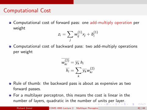
Computational Cost
Computational cost of forward pass: one add-multiply operation perweight
zi =∑j
w(1)ij xj + b
(1)i
Computational cost of backward pass: two add-multiply operationsper weight
w(2)ki = yk hi
hi =∑k
ykw(2)ki
Rule of thumb: the backward pass is about as expensive as twoforward passes.
For a multilayer perceptron, this means the cost is linear in thenumber of layers, quadratic in the number of units per layer.
Richard Zemel COMS 4995 Lecture 2: Multilayer Perceptrons & Backpropagation 42 / 44
Closing Thoughts
Backprop is used to train the overwhelming majority of neural nets today.
Even optimization algorithms much fancier than gradient descent(e.g. second-order methods) use backprop to compute the gradients.
Despite its practical success, backprop is believed to be neurally implausible.
No evidence for biological signals analogous to error derivatives.All the biologically plausible alternatives we know about learn muchmore slowly (on computers).So how on earth does the brain learn?
Richard Zemel COMS 4995 Lecture 2: Multilayer Perceptrons & Backpropagation 43 / 44

Closing Thoughts
The psychological profiling [of a programmer] is mostly the ability to shiftlevels of abstraction, from low level to high level. To see something in the
small and to see something in the large.
– Don Knuth
By now, we’ve seen three different ways of looking at gradients:
Geometric: visualization of gradient in weight spaceAlgebraic: mechanics of computing the derivativesImplementational: efficient implementation on the computer
When thinking about neural nets, it’s important to be able to shiftbetween these different perspectives!
Richard Zemel COMS 4995 Lecture 2: Multilayer Perceptrons & Backpropagation 44 / 44