J. Symbolic Computation (1997) 23, 255–266

Computing Rational Parametrizations of CanalSurfaces

MARTIN PETERNELL AND HELMUT POTTMANN

Institut fur Geometrie, Technische Universitat Wien, A-1040 Wien, Austria

(Received 11 December 1995)

A canal surface is the envelope of a one-parameter set of spheres with radii r(t) andcenters m(t). It is shown that any canal surface to a rational spine curve m(t) and arational radius function r(t) possesses rational parametrizations. We derive algorithmsfor the computation of these parametrizations and put particular emphasis on low degreerepresentations.

c© 1997 Academic Press Limited

1. Introduction

Current CAD systems can represent curves and surfaces only in rational B-spline(NURBS) form ( .Farin, 1994; .Hoschek and Lasser, 1993). On the other hand, certaincurves and surfaces that arise in practical applications such as offsets of rational curvesor surfaces are in general not rational and therefore need to be approximated. This moti-vated .Farouki and Sakkalis (1990) to introduce the so-called Pythagorean-hodograph (PH)curves, which are planar polynomial curves that possess rational offsets. Recent researchon PH curves and their generalizations to the full class of rational curves with rationaloffsets has shown that they are well–suited for practical use (see e.g. .Ait Haddou andBiard, 1995; .Albrecht and Farouki, 1995; .Farouki, 1992; .Lu, 1995a; .Pottmann, 1995a, .band the references therein).

The offset at distance r to a curve m(t) in 3-space can be defined as the envelope ofthe set of spheres with radius r which are centered at m(t). Such a surface is called apipe surface or tubular surface with spine curve m(t). Surprisingly, it turned out thatpipe surfaces with rational spine curve m(t) always admit a rational parameterization( .Lu and Pottmann, 1996). In the present paper, we will generalize this result as follows.Canal surfaces, defined as envelope of a one-parameter set of spheres with a rationalradius function r(t) and centers at a rational curve m(t) can be rationally parametrized.A constructive proof for this result is given, along with other techniques to computerational parametrizations of pipe and canal surfaces with low degree spine curves andradius functions. In practical applications, canal surfaces mainly appear as blend surfacesand transition surfaces between pipes. Note that the present class of surfaces contains asspecial case the Dupin cyclides, which have been proposed by several authors for variousapplications in Computer Aided Geometric Design (see e.g. .Pratt, 1995; .Srinivas andDutta, 1994).

0747–7171/97/020255 + 12 $25.00/0 sy960087 c© 1997 Academic Press Limited

256 M. Peternell and H. Pottmann

2. Geometric Properties of Canal Surfaces

Let R3 be Euclidean 3-space with Cartesian coordinates x1, x2, x3. A point p is rep-resented with respect to a coordinate system by a vector (p1, p2, p3), and in general wedo not distinguish between the point and its coordinate vector. Let P3 be projective3-space. A point p is represented by its homogeneous coordinates p = (p0 : p1 : p2 : p3).If p0 6= 0 the relation between Cartesian and homogeneous coordinates is pi = pi/p0 fori = 1, 2, 3. In general x denotes a Cartesian coordinate vector or point in 3-space. By themap x→ (1, x) we embed R3 into P3. Then the complement of R3 in P3 is the plane atinfinity or ideal plane and the homogeneous coordinates of its points satisfy x0 = 0. TheEuclidean scalar product of two vectors a, b shall be denoted by a · b, the vector productby a× b.

A canal surface Φ is defined as envelope of a one-parameter set of spheres Σ(t), centeredat a spine curve m(t). The radius of the spheres is given by the function r(t), t ∈ R. Thedefining equations for Φ are

Σ(t) : (x−m(t))2 − r(t)2 = 0, (2.1)Σ(t) : (x−m(t)) · m(t) + r(t)r(t) = 0. (2.2)

A canal surface Φ contains a one parameter set of so called characteristic circles k(t) =Σ(t)∩Σ(t). Obviously the plane Σ is perpendicular to the derivative vector m. Eliminationof the parameter t from above equations leads to an equation of Φ. Figure 1 illustratesthat a canal surface Φ can also be interpreted as envelope of a one parameter set of conesof revolution ∆(t). These cones are tangent to Φ at points of the characteristic circlesk(t).

Let q be the unit normals of Φ. For each fixed t0 the vector field q(t0, u) shall representthe unit normals at points of k(t0), such that a parametric representation of Φ is givenby

Φ : x(t, u) = m(t) + r(t)q(t, u). (2.3)

If r ≡ const., Φ is the envelope of a moving sphere and is called a pipe surface. Apipe surface can also be interpreted as the envelope of a one parameter set of congruentcylinders of revolution. The plane Σ intersects Σ in a great circle, centered at m. Thisimplies that a pipe surface is always real.

The reality of a canal surface Φ depends in general on r and the length of m. Substi-tuting y = x−m in (2.1) and (2.2), it follows that (y · m)2 = y2r2. One obtains

1 ≥ cos2 α =(y · m)2

y2m2=

r2

m2. (2.4)

We conclude that the envelope is real, exactly if m2 − r2 ≥ 0.

Remark: If equality holds for a parameter value t0, the plane Σ(t0) is tangent to thesphere Σ(t0), such that k(t0) degenerates to a single point. If equality holds in a non-empty interval, the envelope degenerates to a curve plus the one parameter set of tangentplanes Σ(t).

In the following equality shall hold only for isolated parameter values. For the con-struction of parametrizations it is necessary that (2.4) is true for all real numbers. Incases where the reality condition is satisfied only for t ∈ [a, b] 6= R and a 6= b, one mayuse a reparametrization. For instance, let t = (a + bs2)/(1 + s2), such that the realitycondition holds for all s ∈ R.

Rational Canal Surfaces 257

1

k

mm.

Σ Σ.

r

q

e

α

Φ∆

.

.

.

s

Figure 1. Geometric properties.

Since rationality is quite important for practical use, we only deal with rational spinecurves m(t) and rational radius functions r(t). We introduce two methods deriving ra-tional parametrizations of the form (2.3). In both cases the main problem is to find arational curve contained in Φ. We did a first attempt in Section 3. But the necessaryconditions lead to calculations, which are rather difficult. The second one (Section 5)is more geometric and essentially uses the Gauss map. Further we give a constructiveproof of the existence of rational parametrizations of real canal surfaces determined bya rational spine curve m(t) and a rational radius r(t).

3. System of Quadratic Equations

Let m(t) be a rational spine curve and r(t) a rational radius function. A rationalparametrization of the form (2.3) is given, if it is possible to construct a rational vectorfunction q(t, u) such that x = m + rq satisfies (2.1) and (2.2). The resulting conditionsare q2 ≡ 1 and

q · m+ r ≡ 0, (3.1)

corresponding to equations (2.1) and (2.2). Each characteristic circle k can be paramet-rized in a rational way by a parameter u, described in Section 3.2. The main problemis to determine a unit vector field q(t) which satisfies (3.1), such that f = m + rq is arational curve in Φ.

Since q(t) is a rational curve contained in the unit sphere S2, it follows from .Dietz etal. (1993) that a homogeneous coordinate representation of q is

q0 = p20 + p2

1 + p22 + p2

3, q1 = 2(p0p1 − p2p3),q2 = 2(p0p2 + p1p3), q3 = p2

0 − p21 − p2

2 + p23,

with polynomials p0(t), . . . , p3(t). Assume that the Cartesian coordinate functions mi

and the radius function r are of degree ≤ k and have a common denominator d. Letpi(t) = pi0 + pi1t + · · · + pint

n be polynomials of degree n. Then equation (3.1) is apolynomial of degree 2n + 2k − 2. The identity condition in (3.1) leads to a system of2n+2k−1 equations, quadratic in the 4(n+1) homogeneous unknowns pij for i = 0, 1, 2, 3and j = 0, . . . , n.

If n ≥ k − 2, it would be possible that (3.1) has real solutions. Further the rational

258 M. Peternell and H. Pottmann

c

∆

.

.

g

q~

k

hF

n

m. O

σ1

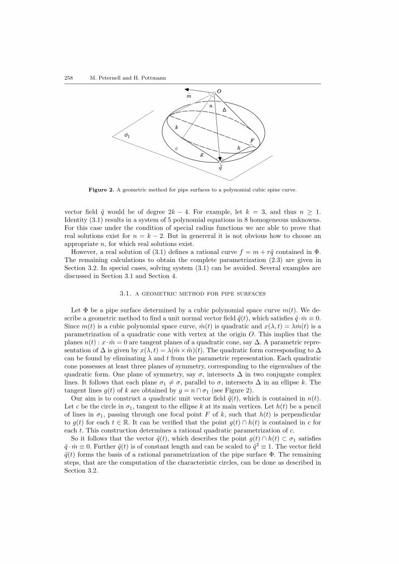
Figure 2. A geometric method for pipe surfaces to a polynomial cubic spine curve.

vector field q would be of degree 2k − 4. For example, let k = 3, and thus n ≥ 1.Identity (3.1) results in a system of 5 polynomial equations in 8 homogeneous unknowns.For this case under the condition of special radius functions we are able to prove thatreal solutions exist for n = k − 2. But in genereral it is not obvious how to choose anappropriate n, for which real solutions exist.

However, a real solution of (3.1) defines a rational curve f = m + rq contained in Φ.The remaining calculations to obtain the complete parametrization (2.3) are given inSection 3.2. In special cases, solving system (3.1) can be avoided. Several examples arediscussed in Section 3.1 and Section 4.

3.1. a geometric method for pipe surfaces

Let Φ be a pipe surface determined by a cubic polynomial space curve m(t). We de-scribe a geometric method to find a unit normal vector field q(t), which satisfies q ·m ≡ 0.Since m(t) is a cubic polynomial space curve, m(t) is quadratic and x(λ, t) = λm(t) is aparametrization of a quadratic cone with vertex at the origin O. This implies that theplanes n(t) : x ·m = 0 are tangent planes of a quadratic cone, say ∆. A parametric repre-sentation of ∆ is given by x(λ, t) = λ(m×m)(t). The quadratic form corresponding to ∆can be found by eliminating λ and t from the parametric representation. Each quadraticcone possesses at least three planes of symmetry, corresponding to the eigenvalues of thequadratic form. One plane of symmetry, say σ, intersects ∆ in two conjugate complexlines. It follows that each plane σ1 6= σ, parallel to σ, intersects ∆ in an ellipse k. Thetangent lines g(t) of k are obtained by g = n ∩ σ1 (see Figure 2).

Our aim is to construct a quadratic unit vector field q(t), which is contained in n(t).Let c be the circle in σ1, tangent to the ellipse k at its main vertices. Let h(t) be a pencilof lines in σ1, passing through one focal point F of k, such that h(t) is perpendicularto g(t) for each t ∈ R. It can be verified that the point g(t) ∩ h(t) is contained in c foreach t. This construction determines a rational quadratic parametrization of c.

So it follows that the vector q(t), which describes the point g(t) ∩ h(t) ⊂ σ1 satisfiesq · m ≡ 0. Further q(t) is of constant length and can be scaled to q2 ≡ 1. The vector fieldq(t) forms the basis of a rational parametrization of the pipe surface Φ. The remainingsteps, that are the computation of the characteristic circles, can be done as described inSection 3.2.

Rational Canal Surfaces 259

mγ

q~

x

.

m.

rf

c

Figure 3. Computing the characteristic circles.

3.2. computing the characteristic circles

Let m(t) and r(t) be rational and assume that q(t) is already computed and definesa rational curve f = m + rq, contained in Φ. For a fixed t0 let γ(t0, u) be the pencilof planes passing through the tangent line m(t0) + λm(t0), as illustrated in Figure 3.Further let c(t0, u) be the normal vectors of γ(t0, u) given by

c(t0, u) = v1(t0) + uv2(t0),

where v1, v2 denote two distinct normal vectors of planes contained in this pencil. Wemay choose v1, v2 in the following way

v1 = (m2,−m1, 0), v2 = (m3, 0,−m1).

Note that singularities may occur, namely for parameter values where v1, v2 are linearlydependent. This can be avoided by c(t, u) = m(t) × n(t) + un(t), where n(t) denotes anormal vector field of the spine curve m(t).

One generates the characteristic circle corresponding to t0 by reflecting f(t0) at allplanes γ(t0, u). This construction leads to the following parametrization of Φ, namely

x(t, u) = f(t)− 2r(t)c(t, u) · q(t)

c(t, u)2c(t, u). (3.2)

We mention that the parameter u varies in R ∪∞.

4. Canal Surfaces Tangent to Special Surfaces

In this section several examples shall be presented, where it is not necessary tosolve (3.1), since a rational curve f ⊂ Φ, different from a characteristic circle is alreadygiven. It follows from (3.2) that Φ is rational. To obtain parametric representations of Φone only has to apply the construction described in Section 3.2 or similar ones.

First we study the class of canal surfaces tangent to a constant plane. This classincludes well-known surfaces like Dupin cyclides. A rational curve f contained in Φ isthe orthogonal projection of the spine curve m onto the constant tangent plane.

Let m(t) be an arbitrary rational curve. Let x3 = 0 be the constant tangent plane.This implies r(t) = m3(t) and with (3.2) the canal surface can be parametrized by

x(t, u) = (m1,m2, 0) + 2c3m3

c21 + c22 + c23(c1, c2, c3). (4.1)

260 M. Peternell and H. Pottmann

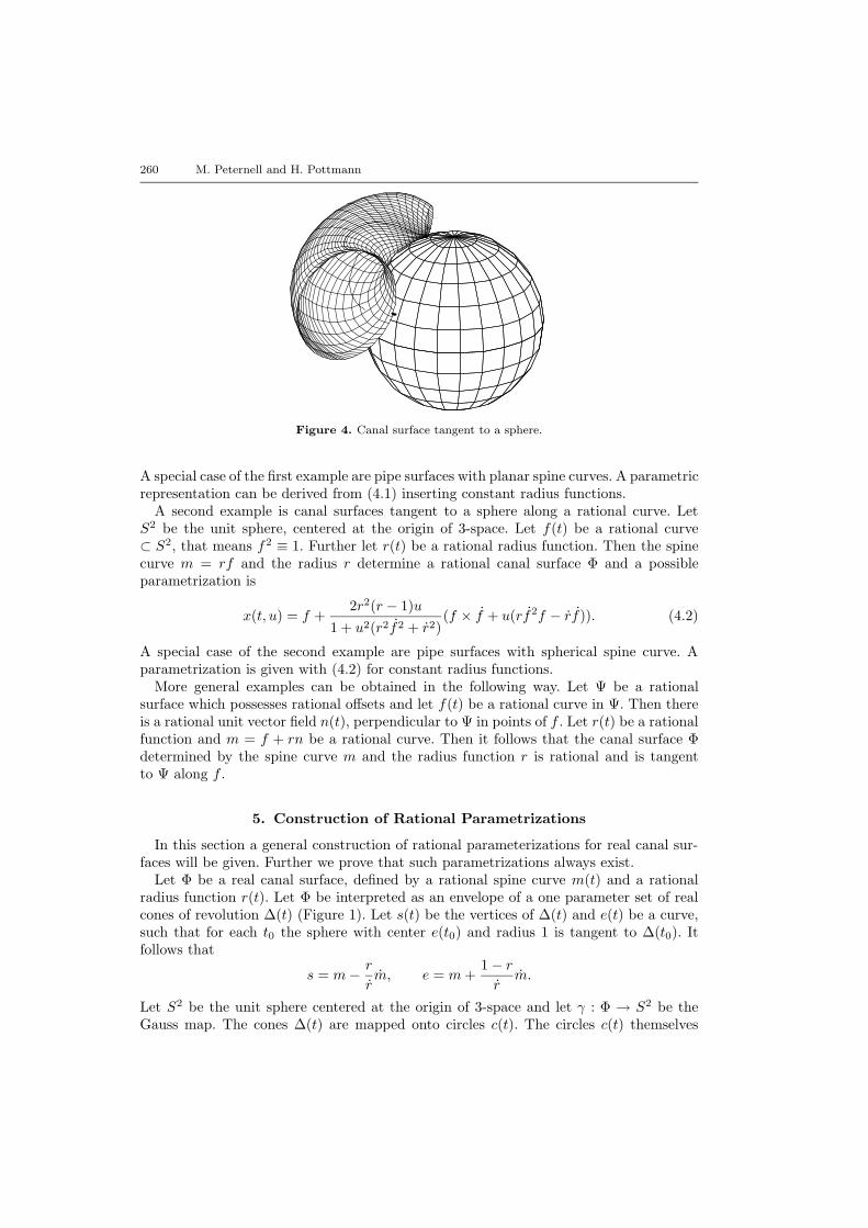
Figure 4. Canal surface tangent to a sphere.

A special case of the first example are pipe surfaces with planar spine curves. A parametricrepresentation can be derived from (4.1) inserting constant radius functions.

A second example is canal surfaces tangent to a sphere along a rational curve. LetS2 be the unit sphere, centered at the origin of 3-space. Let f(t) be a rational curve⊂ S2, that means f2 ≡ 1. Further let r(t) be a rational radius function. Then the spinecurve m = rf and the radius r determine a rational canal surface Φ and a possibleparametrization is

x(t, u) = f +2r2(r − 1)u

1 + u2(r2f2 + r2)(f × f + u(rf2f − rf)). (4.2)

A special case of the second example are pipe surfaces with spherical spine curve. Aparametrization is given with (4.2) for constant radius functions.

More general examples can be obtained in the following way. Let Ψ be a rationalsurface which possesses rational offsets and let f(t) be a rational curve in Ψ. Then thereis a rational unit vector field n(t), perpendicular to Ψ in points of f . Let r(t) be a rationalfunction and m = f + rn be a rational curve. Then it follows that the canal surface Φdetermined by the spine curve m and the radius function r is rational and is tangentto Ψ along f .

5. Construction of Rational Parametrizations

In this section a general construction of rational parameterizations for real canal sur-faces will be given. Further we prove that such parametrizations always exist.

Let Φ be a real canal surface, defined by a rational spine curve m(t) and a rationalradius function r(t). Let Φ be interpreted as an envelope of a one parameter set of realcones of revolution ∆(t) (Figure 1). Let s(t) be the vertices of ∆(t) and e(t) be a curve,such that for each t0 the sphere with center e(t0) and radius 1 is tangent to ∆(t0). Itfollows that

s = m− r

rm, e = m+

1− rr

m.

Let S2 be the unit sphere centered at the origin of 3-space and let γ : Φ → S2 be theGauss map. The cones ∆(t) are mapped onto circles c(t). The circles c(t) themselves

Rational Canal Surfaces 261

define cones of revolution ∆(t), which are tangent to S2 along c(t). The vertices of thecones ∆ are given by z = s− e which leads to

z(t) =−1r(t)

m(t).

Note that z is at infinity, if r = 0.Our aim is to construct a rational unit normal q ⊂ S2 of Φ, such that (2.3) is a rational

parametrization of Φ. For each fixed t0 the vector field q(t0, u) describes a circle ⊂ S2.To derive parametrizations it is comfortable to use a stereographic projection.

Let π be the Euclidean plane in 3-space defined by x3 = 0 and W = (0, 0, 1). Astereographic projection δ : S2 → π with center W is a rational conformal map. Inparticular δ maps circles c to circles or lines δ(c). In general δ(c) is a circle with centern = δ(z) and radius ρ given by

n =−1

r + m3(m1, m2, 0), (5.1)

ρ2 =1

(r + m3)2(m2 − r2). (5.2)

It is clear that δ(c) is a line, exactly if r + m3 = 0. For further calculations one uses aLemma, which can be proved by factorizing the given polynomial over the complex field.

Lemma 5.1. Let f be a real definite polynomial, which means that f(t) ≥ 0 for all t ∈ R.Then there exist polynomials f1, f2, such that f = f2

1 + f22 .

Let us summarize what we have done till now. The stereographic projection of theGauss image of Φ contains a one parameter set of circles δ(c), centered at a rationalplanar curve n(t). But in general the radius function ρ is not rational. A rational curve ϕcorresponding to the set δ(c) shall be constructed, such that for each fixed t0 the pointϕ(t0) is contained in the circle δ(c(t0)). Therefore ϕ has to be of the form

ϕ(t) = n(t) + g(t), (5.3)

where g(t) a rational planar vector, whose coordinates satisfy g21 + g2

2 = ρ2.Since the denominator in (5.2) is a square, it is sufficient to apply Lemma 5.1 to

the numerator of ρ2 ≥ 0. A solution g1, g2 of the decomposition of ρ2 leads to therepresentation (5.3). To derive the complete parametrization of δ(γ(Φ)) one may proceedas follows. Let d(u) = (u, 1) be normals of a pencil of lines. Similar to Section 3.2, arational parametrization of a fixed circle δ(c) can be constructed by reflecting ϕ at alldiameters of δ(c), which leads to

ϕ(t, u) = ϕ(t)− 2g(t) · d(u)d(u)2

d(u). (5.4)

The inverse projection δ−1 : π → S2 maps ϕ to the unit normals

q(t, u) =1

(1 + ϕ21 + ϕ2

2)(2ϕ1, 2ϕ2, ϕ

21 + ϕ2

2 − 1)(t, u), (5.5)

such that x(t, u) = m(t) + r(t)q(t, u) is a rational parametrization of Φ. Let us collectthe derived results.

262 M. Peternell and H. Pottmann

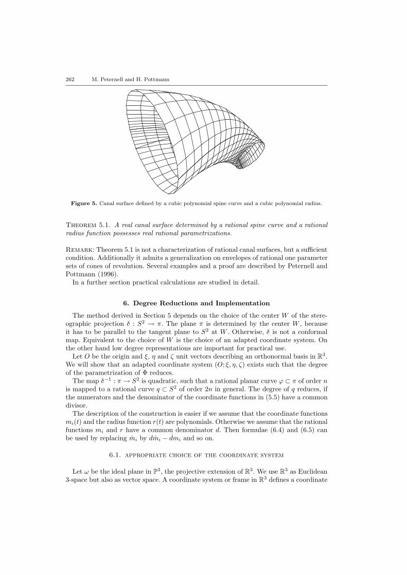
Figure 5. Canal surface defined by a cubic polynomial spine curve and a cubic polynomial radius.

Theorem 5.1. A real canal surface determined by a rational spine curve and a rationalradius function possesses real rational parametrizations.

Remark: Theorem 5.1 is not a characterization of rational canal surfaces, but a sufficientcondition. Additionally it admits a generalization on envelopes of rational one parametersets of cones of revolution. Several examples and a proof are described by .Peternell andPottmann (1996).

In a further section practical calculations are studied in detail.

6. Degree Reductions and Implementation

The method derived in Section 5 depends on the choice of the center W of the stere-ographic projection δ : S2 → π. The plane π is determined by the center W , becauseit has to be parallel to the tangent plane to S2 at W . Otherwise, δ is not a conformalmap. Equivalent to the choice of W is the choice of an adapted coordinate system. Onthe other hand low degree representations are important for practical use.

Let O be the origin and ξ, η and ζ unit vectors describing an orthonormal basis in R3.We will show that an adapted coordinate system (O; ξ, η, ζ) exists such that the degreeof the parametrization of Φ reduces.

The map δ−1 : π → S2 is quadratic, such that a rational planar curve ϕ ⊂ π of order nis mapped to a rational curve q ⊂ S2 of order 2n in general. The degree of q reduces, ifthe numerators and the denominator of the coordinate functions in (5.5) have a commondivisor.

The description of the construction is easier if we assume that the coordinate functionsmi(t) and the radius function r(t) are polynomials. Otherwise we assume that the rationalfunctions mi and r have a common denominator d. Then formulae (6.4) and (6.5) canbe used by replacing mi by dmi − dmi and so on.

6.1. appropriate choice of the coordinate system

Let ω be the ideal plane in P3, the projective extension of R3. We use R3 as Euclidean3-space but also as vector space. A coordinate system or frame in R3 defines a coordinate

Rational Canal Surfaces 263

j

z1 z2

A2

A1

A1 A2

a1

a2

Z2

a2

a1

Z1

V

V

Figure 6. Appropriate choice of the coordinate system.

system in ω. A one-dimensional subspace λv, with λ 6= 0 and v 6= (0, 0, 0) determines apoint V in ω. We may interprete λ(v1, v2, v3) as homogeneous Cartesian coordinates of Vin ω. Let j be the conic in ω defined by x2

1 +x22 +x2

3 = 0. The bilinear form correspondingto j is the Euclidean scalar product x · y = x1y1 + x2y2 + x3y3. The construction of theframe, illustrated in Figure 6, depends essentially on a configuration in ω. Complex linesare represented by dashed lines, real lines by solid lines. Complex points are representedby circles, real points by filled circles.

Let τ, τ be conjugate complex zeros or a real double zero of the definite polynomialf = m2 − r2 ≥ 0, which is the numerator of (5.2). Let v = m(τ) and v = m(τ). Thevectors v and v describe conjugate complex points V, V in ω. Let ai, ai for i = 1, 2 beconjugate complex tangent lines of j, passing through V and V . These lines are tangentto j in points Ai, Ai. A coordinate representation is

Ai = (αi, βi, γi) = (−v1v3 ∓ i v2

√λ,−v2v3 ± i v1

√λ, v2

1 + v22), (6.1)

Ai = (αi, βi, γi) = (−v1v3 ± i v2

√λ,−v2v3 ∓ i v1

√λ, v2

1 + v22), (6.2)

where λ = v · v and λ = v · v . Using the scalar product it follows that the lines ai and aiare represented by the same coordinates as Ai and Ai. That means that ai for instanceis given by the linear equation αix1 + βix2 + γix3 = 0. Further let Zi = ai ∩ ai and let zibe the lines connecting Ai, Ai. It is clear that Zi and zi are real. We choose for instancethe pair Z1, z1 and denote it for simplicity by Z, z. Analogously A, A denote the pointsA1, A1. The point Z and the line z can be represented by the unit vector

ζ = (ζ1, ζ2, ζ3) =A× A‖A× A‖ . (6.3)

The new coordinate system is chosen such that ζ describes the new x3-axis. Let ξ and ηbe unit vectors of the new axes x1, x2. They can be chosen arbitrarily, but have to satisfythe conditions of an orthonormal frame. This implies η = ζ × ξ, where ξ is for instance

ξ1 =ζ2√ζ21 + ζ2

2

, ξ2 = − ζ1√ζ21 + ζ2

2

, ξ3 = 0.

Since this construction depends only on a configuration in ω, the transformation is onlydetermined up to sign changes of the basis vectors. The signs will be determined later.

264 M. Peternell and H. Pottmann

6.2. degree reductions

First we rewrite the formulae of Section 5 in terms of mi and r, assumed to be polyno-mials. Let f1, f2 be polynomials satisfying f2

1 + f22 = m2 − r2. Then the planar rational

curve ϕ is given by

ϕ(t) =1

r + m3(f1 − m1, f2 − m2). (6.4)

Using the following substitutions

e = m21 + m2

2, k = r + m3, g = f1m1 − f2m2, h = f1m2 + f2m1,

and applying (5.4) and (5.5) the homogeneous coordinates of the unit normal q are

q0(t, u) =u2(e+ m3k + g) + 2uh+ e+ m3k − g,q1(t, u) = (−u2(m1 + f1)− 2uf2 + f1 − m1)k,q2(t, u) = (−u2(m2 − f2)− 2uf1 − f2 − m2)k,q3(t, u) =u2(e− rk + g) + 2uh+ e− rk − g.

(6.5)

We use the same notation as in Section 6.1 and assume that a frame is chosen as describedthere, up to the signs of the basis vectors. Let d = (t−τ)(t− τ) and let π : x3 = 0. We willshow that d is a common divisor of the coordinate functions q0, . . . , q3. The orthogonalprojection p : P3 → π with center Z induces a planar projection pω : ω → z in the idealplane. The projection p maps v = m(τ) to p(v) and v = m(τ) to p(v); pω maps V, V toA, A ⊂ j. Since p(v) and p(v) describe the points A and A, which are contained in j, itfollows that p(v)2 = p(v)2 = 0. We see that the polynomial e = p(m)2 has zeros at τand τ , such that d divides e. Since τ and τ are also zeros of m2 − r2 it follows that ddivides m2

3 − r2. We choose the orientation of ζ in (6.3) such that m3(τ) = −r(τ). Thisguarantees that d divides k. Maybe after a substitution of f2 by −f2 we achieve that thereal polynomial d divides the complex polynomial (m1 +i m2)(f1 +i f2). Therefore d alsodivides its real and imaginary parts, g and h, respectively.

We summarize that all coordinate functions qi have a common divisor, such that thedegree of the Cartesian coordinates qi = qi/q0 reduces.

Corollary 6.1. Let Φ be a real canal surface determined by a polynomial spine curvem(t) of degree k and a polynomial radius function r(t) of degree k. Then there exists aunit normal vector function q(t, u) of Φ, which is of degree 2k − 4 in t. The resultingparametrization (m+ rq)(t, u) of Φ is in general of degree 3k − 4 in t and 2 in u.

Let Φ be defined by rational but not polynomial functions mi(t) and r(t) both ofdegree k, which possess a common denominator. The numerators of m and r are ofdegree 2k − 2 and it follows that the normal field q(t, u) is of degree 4k − 6 in t. Theresulting parametrization (m+rq)(t, u) of Φ is in general of degree 5k−6 in t and 2 in u.

Several problems occur when implementing the algorithm given above. One of them isthe decomposition described in Lemma 5.1. In general one has to use numerical methodsto calculate the zeros of f such that the solution f1, f2 is not exact. Further it is clearthat (t− τ)(t− τ) is not an exact divisor of the occuring polynomials. So it is necessaryto combine algebraic and numerical methods (.Stetter, 1996).

A further problem is the distribution of the rational parameter lines f(t, u0) = (m +rq)(t, u0) for a fixed u0 on a canal surface Φ (see Figures 5 and 7). Let Φ be a pipe

Rational Canal Surfaces 265

Figure 7. Pipe surface defined by a cubic polynomial spine curve.

surface. In general the distance between two fixed rational parameter lines f(t, u1) andf(t, u2), measured along the characteristic circles, is not constant. This fact can producerational parametrizations, which are nearly singular. To avoid this one can restrict m(t)to be contained in the class of curves, whose tangent vector m(t) has rational length (see.Farouki and Sakkalis, 1994).

Finally, we would like to mention that .Lu (1995b) has presented a different proof ofthe theorem along with another algorithm to construct rational parametrizations of canalsurfaces. His method leads in general to higher degrees. Another contribution on this topicis a paper by .Malosse (1996). He mainly studies pipe surfaces and the generalization tocanal surfaces is not really straightforward. Furthermore we believe that our algorithmis easier to understand and to implement.

Acknowledgement

This work has been supported by the Austrian Science Foundation through projectP09790–MAT.

References

.—.—Ait Haddou, R., Biard, L. (1995). G2 approximation of an offset curve by Tschirnhausen quartics. In:Daehlen, M., Lyche, T., Schumaker, L.L., eds, Mathematical Methods for Curves and Surfaces,Vanderbilt University Press, 1–10.

.—.—Albrecht, G., Farouki, R.T. (1995). Construction of C2 Pythagorean-hodograph interpolating splines bythe homotopy method. Advances in Comp. Math., to appear.

.—.—Dietz, R., Hoschek, J., Juttler, B. (1993). An algebraic approach to curves and surfaces on the sphereand other quadrics. Comput. Aided Geom. Design 10, 211–229.

.—.—Farin, G. (1994). NURBS for Rational Curve and Surface Design. Wellesley: AK Peters.

.—.—Farouki, R.T., Sakkalis, T. (1990). Pythagorean hodographs. IBM J. Res. Develop. 34, 736–752.

.—.—Farouki, R.T., Sakkalis, T. (1994). Pythagorean hodograph space curves. Adv. in Comp. Math. 2, 41–66.

.—.—Farouki, R.T. (1992). Pythagorean-hodograph curves in practical use. In: Barnhill, R.E., ed., GeometryProcessing for Design and Manufacturing, Philadelphia: SIAM, 3–33.

.—.—Hoschek, J., Lasser, D. (1993). Fundamentals of Computer Aided Geometric Design. Wellesley: AKPeters.

.—.—Lu, W. (1995a). Offset-rational parametric plane curves. Comput. Aided Geom. Design 12, 601–616.

.—.—Lu, W. (1995b). Rational canal surfaces. Technical Report No. 26, Inst. fur Geometrie, TU Wien.

.—.—Lu, W., Pottmann, H. (1996). Pipe surfaces with rational spine curve are rational. Comput. Aided Geom.Design 13.

.—.—Malosse, J.J. (1996). Exact parametrizations of pipe surfaces. submitted to Comput. Aided Geom. De-sign.

.—.—Peternell, M., Pottmann, H. (1997). A Laguerre geometric approach to rational offsets. Comput. AidedGeom. Design, to appear.

266 M. Peternell and H. Pottmann

.—.—Pottmann, H. (1995a). Rational curves and surfaces with rational offsets. Comput. Aided Geom. Design12, 175-192.

.—.—Pottmann, H. (1995b). Curve design with rational Pythagorean-hodograph curves. Adv. in Comp. Math.3, 147–170.

.—.—Pratt, M.J. (1995). Cyclides in Computer Aided Geometric Design II. Comput. Aided Geom. Design 12,131–152.

.—.—Srinivas, Y.L., Dutta, D. (1994). An intuitive procedure for constructing geometrically complex objectsusing cyclides. Computer Aided Design 26, 327–335.

.—.—Stetter, H.J. (1996). Lectures on computational nonlinear algebra. Lecture at TU Vienna, 1996.