Embed Size (px)
Citation preview
COMPUTING GALOIS COHOMOLOGY AND
FORMS OF LINEAR ALGEBRAIC GROUPS
PROEFSCHRIFT
Sergei Haller
CIP-DATA LIBRARY TECHNISCHE UNIVERSITEIT EINDHOVEN
Haller, Sergei
Computing Galois cohomology and forms of linear algebraic groups /Haller, Sergei – Eindhoven: Technische Universiteit Eindhoven, 2005.Proefschrift – ISBN 90-386-0664-8
NUR 921
Subject headings : group theory / linear algebraic groups / cohomology /computer algebra2000 Mathematics Subject Classification: 20G15, 20G40, 11E72, 20G10, 20J06.
Printed by Universiteitsdrukkerij Technische Universiteit EindhovenCover by Jan-Willem Luiten, JWL Producties

COMPUTING GALOIS COHOMOLOGY AND
FORMS OF LINEAR ALGEBRAIC GROUPS
PROEFSCHRIFT
ter verkrijging van de graad van doctor aan de Technische
Universiteit Eindhoven, op gezag van de Rector Magnificus,
prof.dr.ir. C.J. van Duijn, voor een commissie aangewezen
door het College voor Promoties in het openbaar te verdedigen
op woensdag 12 oktober 2005 om 16.00 uur
door
Sergei Haller
geboren te Krasnoturinsk, Rusland

Dit proefschrift is goedgekeurd door de promotoren:
prof.dr. A.M. Cohenenprof. Dr. F.G. Timmesfeld
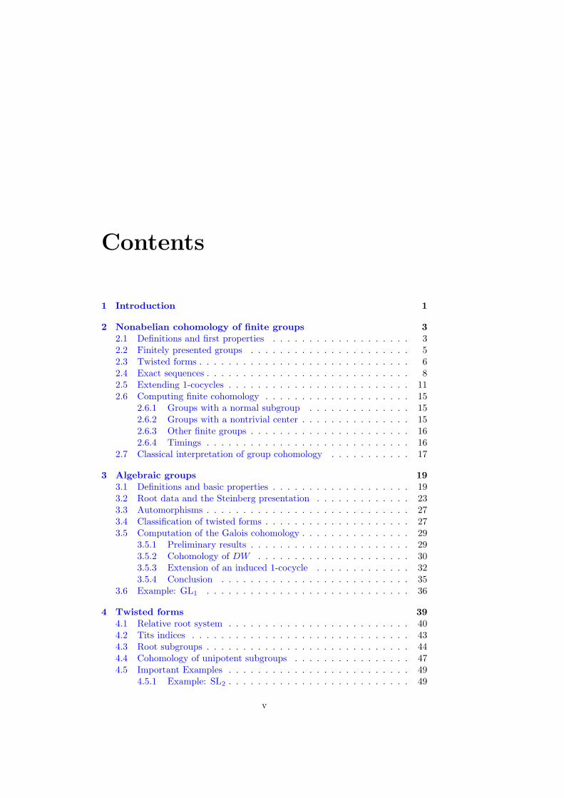
Contents
1 Introduction 1
2 Nonabelian cohomology of finite groups 32.1 Definitions and first properties . . . . . . . . . . . . . . . . . . . 32.2 Finitely presented groups . . . . . . . . . . . . . . . . . . . . . . 52.3 Twisted forms . . . . . . . . . . . . . . . . . . . . . . . . . . . . . 62.4 Exact sequences . . . . . . . . . . . . . . . . . . . . . . . . . . . . 82.5 Extending 1-cocycles . . . . . . . . . . . . . . . . . . . . . . . . . 112.6 Computing finite cohomology . . . . . . . . . . . . . . . . . . . . 15
2.6.1 Groups with a normal subgroup . . . . . . . . . . . . . . 152.6.2 Groups with a nontrivial center . . . . . . . . . . . . . . . 152.6.3 Other finite groups . . . . . . . . . . . . . . . . . . . . . . 162.6.4 Timings . . . . . . . . . . . . . . . . . . . . . . . . . . . . 16
2.7 Classical interpretation of group cohomology . . . . . . . . . . . 17
3 Algebraic groups 193.1 Definitions and basic properties . . . . . . . . . . . . . . . . . . . 193.2 Root data and the Steinberg presentation . . . . . . . . . . . . . 233.3 Automorphisms . . . . . . . . . . . . . . . . . . . . . . . . . . . . 273.4 Classification of twisted forms . . . . . . . . . . . . . . . . . . . . 273.5 Computation of the Galois cohomology . . . . . . . . . . . . . . . 29
3.5.1 Preliminary results . . . . . . . . . . . . . . . . . . . . . . 293.5.2 Cohomology of DW . . . . . . . . . . . . . . . . . . . . . 303.5.3 Extension of an induced 1-cocycle . . . . . . . . . . . . . 323.5.4 Conclusion . . . . . . . . . . . . . . . . . . . . . . . . . . 35
3.6 Example: GL1 . . . . . . . . . . . . . . . . . . . . . . . . . . . . 36
4 Twisted forms 394.1 Relative root system . . . . . . . . . . . . . . . . . . . . . . . . . 404.2 Tits indices . . . . . . . . . . . . . . . . . . . . . . . . . . . . . . 434.3 Root subgroups . . . . . . . . . . . . . . . . . . . . . . . . . . . . 444.4 Cohomology of unipotent subgroups . . . . . . . . . . . . . . . . 474.5 Important Examples . . . . . . . . . . . . . . . . . . . . . . . . . 49
4.5.1 Example: SL2 . . . . . . . . . . . . . . . . . . . . . . . . . 49
v
Sergei Haller
4.5.2 A twisted form of E6 of rank 1: 2E356,1(k) . . . . . . . . . . 534.5.3 The groups 3D4,1(k) and
6D4,1(k) . . . . . . . . . . . . . 554.5.4 2A7(k) inside E7(k) . . . . . . . . . . . . . . . . . . . . . 57
5 Maximal tori and Sylow subgroups 615.1 Twisted maximal tori . . . . . . . . . . . . . . . . . . . . . . . . 615.2 Rational maximal tori . . . . . . . . . . . . . . . . . . . . . . . . 635.3 Generators of twisted tori . . . . . . . . . . . . . . . . . . . . . . 645.4 Computing orders of the maximal tori . . . . . . . . . . . . . . . 655.5 Computation of Sylow p-subgroups . . . . . . . . . . . . . . . . . 67
A Decomposition of orders of maximal tori 69A.1 How to read the tables . . . . . . . . . . . . . . . . . . . . . . . . 69A.2 Tables . . . . . . . . . . . . . . . . . . . . . . . . . . . . . . . . . 70
Bibliography 79
Index 83
Samenvatting 87
Acknowledgments 89
Curriculum Vitae 91
vi
Sergei Haller
Notation
Here, we describe some common notation used throughout this work. Given
elements g and h of the group G, we write
gh := h−1gh and hg := hgh−1
for right and left conjugation. For a subgroup H of G, we write CG(H) for the
centralizer of H in G, NG(H) for normalizer of H in G, and Z(G) for the center
of G.
For a given field k, we denote its multiplicative group by k∗. Mn(k) is the set
of all n × n matrices with entries in k. We denote the algebraic and separable
closures of k by k and ksep, respectively.
We finish complete proofs with ¤ and incomplete proofs with ¥. In the latter
case, a reference to a complete proof is given. Known results are indicated as
such by giving a reference after the statement.
vii
Chapter 1
Introduction
Computations with large finite or infinite groups are usually very tedious and
time consuming. In many cases the computations carried out are very me-
chanical and error prone when carried out by hand. Such computations can
often be carried out more easily by computer. For more complicated tasks
one needs to design and implement new algorithms. For groups in particular,
this includes operations with group elements (multiplication, inversion, conjuga-
tion, etc.) or other important properties (subgroup structure, conjugacy classes,
etc.). The first problem is deciding how elements should be represented in the
computer. Often a group is defined intrinsically, that is, defined implicitly by
requiring some properties on the elements (e.g., the fixed point subgroup of an-
other group). For computations with group elements, such a definition is not
very useful, since it provides no group elements other than the identity. In such
cases one needs an extrinsic definition for the group, such as a presentation or
a matrix representation.
We design and implement algorithms for computation with groups of Lie type.
Algorithms for element arithmetic in the Steinberg presentation of untwisted
groups of Lie type, and for conversion between this presentation and linear
representations, were given in [12] (building on work of [15] and [26]). We
extend this work to twisted groups, including groups that are not quasisplit.
A twisted group of Lie type is the group of rational points of a twisted form
of a reductive linear algebraic group. These forms are classified by Galois coho-
mology. In order to compute the Galois cohomology, we develop a method for
computing the cohomology of a finitely presented group Γ on a finite group A.
This method is of interest in its own right. We then extend this method to the
Galois cohomology of reductive linear algebraic groups.
Let G be a reductive linear algebraic group defined over a field k. A twisted
group of Lie type Gα(k) is uniquely determined by the cocycle α of the Galois
group of K on A := AutK(G), the group of K-algebraic automorphisms where
1
Sergei Haller 1. Introduction
K is a finite Galois extension of k. We give algorithms for computing the
relative root system of Gα(k), the root subgroups, and the root elements, as
well as algorithms for the computing of relations between root elements. This
enables us to compute inside the normal subgroup Gα(k)† of Gα(k) generated
by the root elements. We apply our algorithms to several examples, including2E6,1(k) and 3,6D4,1(k). In this application, the field k need not be specified,
one only needs to assume some properties of k.
As an application, we develop an algorithm for computing all twisted maximal
tori of a finite group of Lie type. The order of such a torus is computed as a
polynomial in q, the order of the field k. We also compute the orders of the
factors in a decomposition of the torus as a direct product of cyclic subgroups.
For a given field k, we compute the maximal tori of Gβ(k) as subgroups of
Gβ(K) over some extension field K, and then use the effective version of Lang’s
Theorem [11] to conjugate the torus to a k-torus, which is a subgroup of Gβ(k).
Using this information on the maximal tori, we provide an algorithm for
computing all Sylow subgroups of a finite group of Lie type. If p is not the
characteristic of the field, the Sylow subgroup is computed as a subgroup of the
normaliser of a k-torus.
All algorithms presented here have been implemented by the author in Magma
[5].
2

Chapter 2
Nonabelian cohomology of
finite groups
We are primarily interested in the twisted forms of linear algebraic groups, which
are classified via the Galois cohomology. In the present chapter, we introduce
the first cohomology of nonabelian groups and develop a new technique for
computing cohomology H1(Γ, A) for a finitely presented group Γ and a finite
group A. In Chapter 3, we extend this technique to Galois cohomology. We
also introduce the concept of twisting in Section 2.3.
2.1 Definitions and first properties
Let Γ be a group. A Γ-set A is a set with a (right) Γ-action. If A is a group
and Γ acts by group automorphisms, then A is called a Γ-group. A subset
(subgroup) of the Γ-set (Γ-group) A that is normalised by the action of Γ, is
called a Γ-subset (Γ-subgroup) of A. Given a Γ-set A, define
H0(Γ, A) := {a ∈ A | aσ = a for all σ ∈ Γ}.
If A is a Γ-group, then H0(Γ, A) is a subgroup of A.
Now let A be a Γ-group. A 1-cocycle of Γ on A is a map
α : Γ→ A, σ 7→ ασ,
such that
αστ = (ασ)τατ for all σ, τ ∈ Γ. (2.1)
We denote by Z1(Γ, A) the set of all 1-cocycles of Γ on A. The constant map
1 : σ 7→ 1 is a distinguished element of Z1(Γ, A), called the trivial 1-cocycle.
3
Sergei Haller 2. Nonabelian cohomology of finite groups
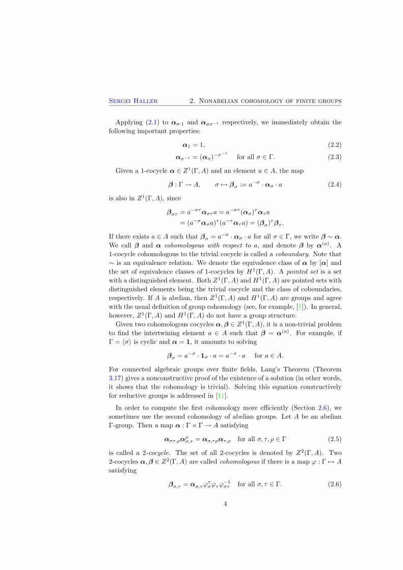
Applying (2.1) to ασ·1 and ασσ−1 respectively, we immediately obtain the
following important properties:
α1 = 1, (2.2)
ασ−1 = (ασ)−σ−1
for all σ ∈ Γ. (2.3)
Given a 1-cocycle α ∈ Z1(Γ, A) and an element a ∈ A, the map
β : Γ→ A, σ 7→ βσ := a−σ ·ασ · a (2.4)
is also in Z1(Γ, A), since
βστ = a−σταστa = a−στ (ασ)τατa
= (a−σασa)τ (a−τατa) = (βσ)
τβτ .
If there exists a ∈ A such that βσ = a−σ ·ασ · a for all σ ∈ Γ, we write β ∼ α.
We call β and α cohomologous with respect to a, and denote β by α(a). A
1-cocycle cohomologous to the trivial cocycle is called a coboundary. Note that
∼ is an equivalence relation. We denote the equivalence class of α by [α] and
the set of equivalence classes of 1-cocycles by H1(Γ, A). A pointed set is a set
with a distinguished element. Both Z1(Γ, A) and H1(Γ, A) are pointed sets with
distinguished elements being the trivial cocycle and the class of coboundaries,
respectively. If A is abelian, then Z1(Γ, A) and H1(Γ, A) are groups and agree
with the usual definition of group cohomology (see, for example, [1]). In general,
however, Z1(Γ, A) and H1(Γ, A) do not have a group structure.
Given two cohomologous cocycles α,β ∈ Z1(Γ, A), it is a non-trivial problem
to find the intertwining element a ∈ A such that β = α(a). For example, if
Γ = 〈σ〉 is cyclic and α = 1, it amounts to solving
βσ = a−σ · 1σ · a = a−σ · a for a ∈ A.
For connected algebraic groups over finite fields, Lang’s Theorem (Theorem
3.17) gives a nonconstructive proof of the existence of a solution (in other words,
it shows that the cohomology is trivial). Solving this equation constructively
for reductive groups is addressed in [11].
In order to compute the first cohomology more efficiently (Section 2.6), we
sometimes use the second cohomology of abelian groups. Let A be an abelian
Γ-group. Then a map α : Γ× Γ→ A satisfying
αστ,ραρσ,τ = ασ,τρατ,ρ for all σ, τ, ρ ∈ Γ (2.5)
is called a 2-cocycle. The set of all 2-cocycles is denoted by Z2(Γ, A). Two
2-cocycles α,β ∈ Z2(Γ, A) are called cohomologous if there is a map ϕ : Γ 7→ A
satisfying
βσ,τ = ασ,τϕτσϕτϕ
−1στ for all σ, τ ∈ Γ. (2.6)
4
2.2. Finitely presented groups Sergei Haller
This is an equivalence relation, whose set of equivalence classes is denoted
H2(Γ, A). Once again, there is a trivial 2-cocycle, denoted 1.
Let M,N be two pointed sets. A map ϕ : M → N is called a morphism
of pointed sets if it maps the distinguished element of M to the distinguished
element of N . Let A and B be Γ-groups and let φ : A → B be a group
homomorphism. We call φ a Γ-homomorphism if it respects the Γ-action, i.e.,
(aσ)φ =(
aφ)σ
for all σ ∈ Γ and a ∈ A.
If φ : A→ B is a Γ-homomorphism, it is immediate from the definitions that
there are induced maps
φi : Zi(Γ, A)→ Zi(Γ, B) (i = 1),
φi : Hi(Γ, A)→ Hi(Γ, B) (i = 0, 1).
Note that we use the same name φ1 for the maps Z1(Γ, A) → Z1(Γ, B) and
H1(Γ, A) → H1(Γ, B), since it is obvious from context which one is intended.
Moreover, φ0 is a group homomorphism and φ1 is a morphism of pointed sets. If
A and B are abelian Γ-groups, there are also induced maps φ2, and the maps φ1
and φ2 are group homomorphisms. If ψ : B → C is another Γ-homomorphism,
then the functorial property
(φψ)i = φiψi
holds for all i = 0, 1, 2 whenever the maps are defined.
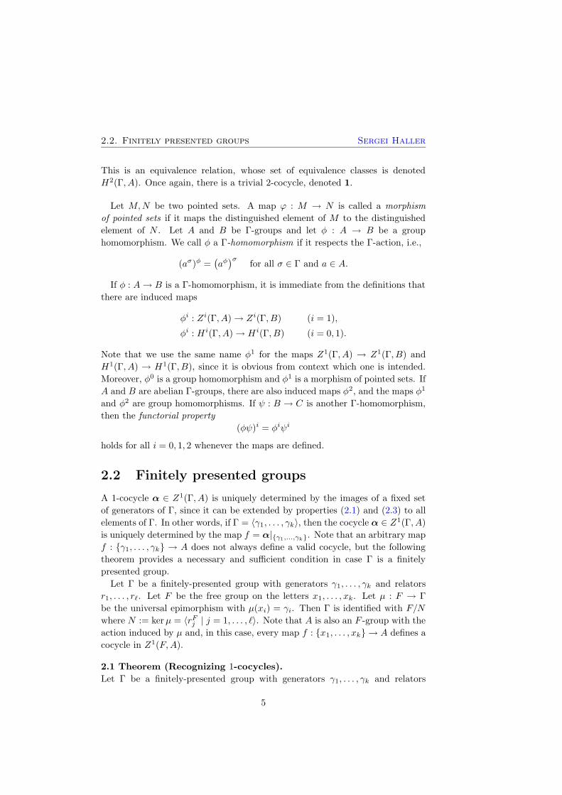
2.2 Finitely presented groups
A 1-cocycle α ∈ Z1(Γ, A) is uniquely determined by the images of a fixed set
of generators of Γ, since it can be extended by properties (2.1) and (2.3) to all
elements of Γ. In other words, if Γ = 〈γ1, . . . , γk〉, then the cocycle α ∈ Z1(Γ, A)is uniquely determined by the map f = α|{γ1,...,γk}. Note that an arbitrary map
f : {γ1, . . . , γk} → A does not always define a valid cocycle, but the following
theorem provides a necessary and sufficient condition in case Γ is a finitely
presented group.
Let Γ be a finitely-presented group with generators γ1, . . . , γk and relators
r1, . . . , r`. Let F be the free group on the letters x1, . . . , xk. Let µ : F → Γ
be the universal epimorphism with µ(xi) = γi. Then Γ is identified with F/N
where N := kerµ = 〈rFj | j = 1, . . . , `〉. Note that A is also an F -group with the
action induced by µ and, in this case, every map f : {x1, . . . , xk} → A defines a
cocycle in Z1(F,A).
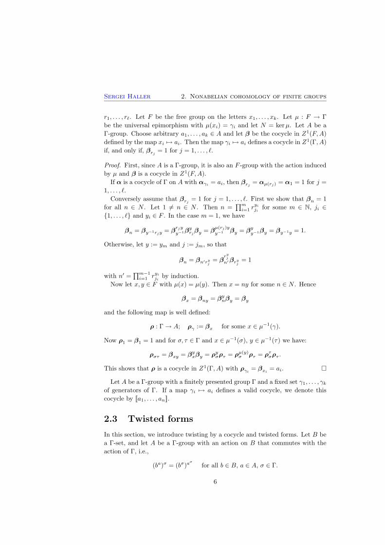
2.1 Theorem (Recognizing 1-cocycles).
Let Γ be a finitely-presented group with generators γ1, . . . , γk and relators
5
Sergei Haller 2. Nonabelian cohomology of finite groups
r1, . . . , r`. Let F be the free group on the letters x1, . . . , xk. Let µ : F → Γ
be the universal epimorphism with µ(xi) = γi and let N = kerµ. Let A be a
Γ-group. Choose arbitrary a1, . . . , ak ∈ A and let β be the cocycle in Z1(F,A)
defined by the map xi 7→ ai. Then the map γi 7→ ai defines a cocycle in Z1(Γ, A)
if, and only if, βrj = 1 for j = 1, . . . , `.
Proof. First, since A is a Γ-group, it is also an F -group with the action induced
by µ and β is a cocycle in Z1(F,A).
If α is a cocycle of Γ on A with αγi = ai, then βrj = αµ(rj) = α1 = 1 for j =
1, . . . , `.
Conversely assume that βrj = 1 for j = 1, . . . , `. First we show that βn = 1
for all n ∈ N . Let 1 6= n ∈ N . Then n =∏mi=1 r
yiji
for some m ∈ N, ji ∈{1, . . . , `} and yi ∈ F . In the case m = 1, we have
βn = βy−1rjy = βrjy
y−1βyrjβy = β
µ(rj)y
y−1 βy = βyy−1βy = βy−1y = 1.
Otherwise, let y := ym and j := jm, so that
βn = βn′ryj= β
ryjn′βryj
= 1
with n′ =∏m−1i=1 ryiji by induction.
Now let x, y ∈ F with µ(x) = µ(y). Then x = ny for some n ∈ N . Hence
βx = βny = βynβy = βy
and the following map is well defined:
ρ : Γ→ A; ργ := βx for some x ∈ µ−1(γ).
Now ρ1 = β1 = 1 and for σ, τ ∈ Γ and x ∈ µ−1(σ), y ∈ µ−1(τ) we have:
ρστ = βxy = βyxβy = ρyσρτ = ρµ(y)σ ρτ = ρτσρτ .
This shows that ρ is a cocycle in Z1(Γ, A) with ργi = βxi = ai. ¤
Let A be a Γ-group with a finitely presented group Γ and a fixed set γ1, . . . , γkof generators of Γ. If a map γi 7→ ai defines a valid cocycle, we denote this
cocycle by [[a1, . . . , an]].
2.3 Twisted forms
In this section, we introduce twisting by a cocycle and twisted forms. Let B be
a Γ-set, and let A be a Γ-group with an action on B that commutes with the
action of Γ, i.e.,
(ba)σ = (bσ)aσ
for all b ∈ B, a ∈ A, σ ∈ Γ.
6
2.3. Twisted forms Sergei Haller
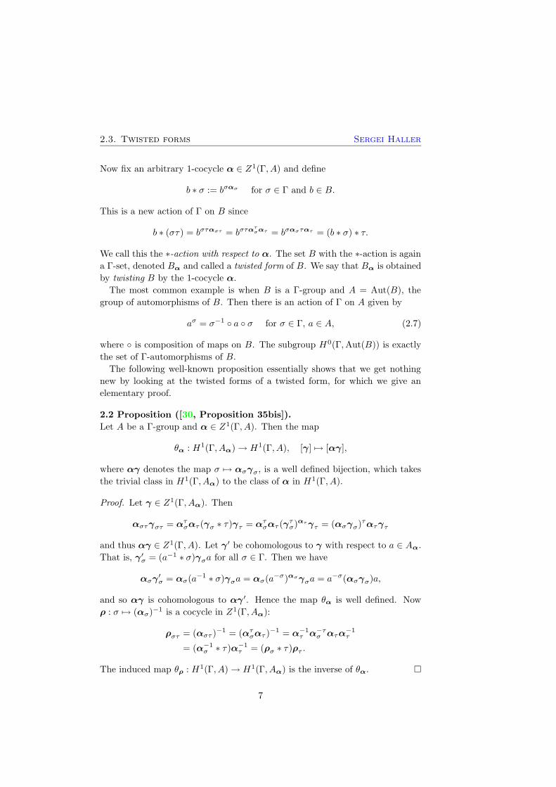
Now fix an arbitrary 1-cocycle α ∈ Z1(Γ, A) and define
b ∗ σ := bσασ for σ ∈ Γ and b ∈ B.
This is a new action of Γ on B since
b ∗ (στ) = bσταστ = bστατσατ = bσαστατ = (b ∗ σ) ∗ τ.
We call this the ∗-action with respect to α. The set B with the ∗-action is again
a Γ-set, denoted Bα and called a twisted form of B. We say that Bα is obtained
by twisting B by the 1-cocycle α.
The most common example is when B is a Γ-group and A = Aut(B), the
group of automorphisms of B. Then there is an action of Γ on A given by
aσ = σ−1 ◦ a ◦ σ for σ ∈ Γ, a ∈ A, (2.7)
where ◦ is composition of maps on B. The subgroup H0(Γ,Aut(B)) is exactly
the set of Γ-automorphisms of B.
The following well-known proposition essentially shows that we get nothing
new by looking at the twisted forms of a twisted form, for which we give an
elementary proof.
2.2 Proposition ([30, Proposition 35bis]).
Let A be a Γ-group and α ∈ Z1(Γ, A). Then the map
θα : H1(Γ, Aα)→ H1(Γ, A), [γ] 7→ [αγ],
where αγ denotes the map σ 7→ ασγσ, is a well defined bijection, which takes
the trivial class in H1(Γ, Aα) to the class of α in H1(Γ, A).
Proof. Let γ ∈ Z1(Γ, Aα). Then
αστγστ = ατσατ (γσ ∗ τ)γτ = ατ
σατ (γτσ)ατγτ = (ασγσ)
τατγτ
and thus αγ ∈ Z1(Γ, A). Let γ′ be cohomologous to γ with respect to a ∈ Aα.
That is, γ′σ = (a−1 ∗ σ)γσa for all σ ∈ Γ. Then we have
ασγ′σ = ασ(a
−1 ∗ σ)γσa = ασ(a−σ)ασγσa = a−σ(ασγσ)a,
and so αγ is cohomologous to αγ ′. Hence the map θα is well defined. Now
ρ : σ 7→ (ασ)−1 is a cocycle in Z1(Γ, Aα):
ρστ = (αστ )−1 = (ατ
σατ )−1 = α−1
τ α−τσ ατα
−1τ
= (α−1σ ∗ τ)α−1
τ = (ρσ ∗ τ)ρτ .
The induced map θρ : H1(Γ, A)→ H1(Γ, Aα) is the inverse of θα. ¤
7
Sergei Haller 2. Nonabelian cohomology of finite groups
2.4 Exact sequences
In this section, we prove a fundamental result for the study of cohomology.
First we need some basic terminology for pointed sets. The kernel ker(µ) of
a morphism of pointed sets µ :M → N is the set of all elements in M mapped
to the distinguished point of N . A sequence of morphisms of pointed sets
Lν→M
µ→ N
is called exact atM if im(ν) = ker(µ). Thus, the sequenceMµ→ N → 1 is exact
if, and only if, µ is surjective, and the sequence 1 → Mµ→ N is exact if, and
only if, ker(µ) contains only the distinguished point of M . Note that this does
not necessarily imply that µ is injective.
The following proposition is well known. Since this proposition is of a funda-
mental nature, we give a detailed proof.
2.3 Proposition ([30, Propositions 36, 38, 43]).
Let A be a Γ-group and let B be a Γ-subgroup of A. Let i : B → A be the
inclusion map. Then A/B is a Γ-set with the natural action of Γ on cosets, and
it is a Γ-group if B is normal. Let π : A → A/B be the canonical projection
map.
(i) Define
δ0 : H0(Γ, A/B)→ H1(Γ, B), aB 7→ [α],
where α is the cocycle defined by ασ := a−σa. Then δ0 is a map of
pointed sets and the sequence
1→ H0(Γ, B)i0→ H0(Γ, A)
π0
→ H0(Γ, A/B)δ0→ H1(Γ, B)
i1→ H1(Γ, A)
is exact.
(ii) If B is normal, the sequence obtained from the sequence in (i) by adding
. . .π1
→ H1(Γ, A/B)
on the right is exact.
(iii) Suppose B is a subgroup of the center of A. Given γ ∈ Z1(Γ, A/B), choose
a map t : Γ→ A with tσ ∈ γσ for every σ ∈ Γ. Set ασ,τ := tτσtτ t−1στ . Then
δ1 : H1(Γ, A/B)→ H2(Γ, B), [γ] 7→ [α]
is a map of pointed sets and the sequence obtained from the sequence in
(ii) by adding
. . .δ1→ H2(Γ, B)
on the right is exact.
8

2.4. Exact sequences Sergei Haller
Proof.
(i) Given a coset aB in A/B, the cocycles defined by ασ := a−σa and βσ :=
(ab)−σ(ab) are obviously cohomologous, thus δ0 is well defined. Moreover,
δ0(A) = [1].
Exactness at H0(Γ, B) is obvious since i0 is just the inclusion map. For
exactness at H0(Γ, A), suppose a ∈ ker(π0). Then π0(a) = B and a ∈ B.
If, on the other hand, a ∈ B, then a obviously lies in the kernel of π0.
For exactness at H0(Γ, A/B), suppose that the cocycle ασ = a−σa is
trivial in H1(Γ, B). That is, α ∼ 1 and ασ = b−σb for some b ∈ B. Then
ab−1 ∈ H0(Γ, A) and aB = (ab−1)B = π0(ab−1) ∈ im(π0).
Finally, let [α] ∈ ker(i1). Then α ∈ Z1(Γ, B) and α is cohomologous to
1 ∈ Z1(Γ, A): ασ = a−σa for some a ∈ A. But this implies (aB)σ =
aσB = (a(ασ)−1)B = aB, thus aB ∈ H0(Γ, A/B) and δ0(aB) = [α]. If,
on the other hand, [α] = δ0(aB) for some a ∈ A, then ασ = a−σa is
cohomologous to 1 ∈ Z1(Γ, A) and [α] ∈ ker(i1).
(ii) Now let α ∈ Z1(Γ, A) with [α] ∈ ker(π1). That means [π1(α)] = [1] ∈H1(Γ, A/B):
ασB = (aB)−σB(aB) = a−σaB = a−σBa for some a ∈ A.
Hence for all σ ∈ Γ we have ασ = a−σbσa for some bσ ∈ B. Now the
map b : Γ → B defined by σ 7→ bσ turns out to be a cocycle on B:
bσ = aσασa−1. Thus [α] = [b] ∈ H1(Γ, A) is the image of [b] ∈ H1(Γ, B)
under the map i1.
(iii) First we show that α ∈ Z2(Γ, B):
(tτσtτ t−1στ )B = tτσBtτBt
−1στB = γτσγτγ
−1στ = 1A/B = B
and thus ασ,τ ∈ B for all σ, τ ∈ Γ. Now we prove the cocycle condition
(note that expressions in parenthesis are in B and thus commute with all
elements):
αστ,ραρσ,τ = (tρστ tρt
−1στρ)(t
τρσ t
ρτ t
−ρστ ) = (tτρσ t
ρτ t
−ρστ )(t
ρστ tρt
−1στρ)
= tτρσ tρτ tρt
−1στρ = tτρσ (tρτ tρt
−1τρ )tτρt
−1στρ = tτρσ tτρt
−1στρ(t
ρτ tρt
−1τρ )
= ασ,τρατ,ρ.
Moreover, if we choose a different map t′ : Γ→ A with t′σ ∈ γσ for every
σ ∈ Γ, then t′σ = tσbσ for some bσ ∈ B and the obtained 2-cocycle α′ is
cohomologous to α:
α′σ,τ = (t′σ)
τ t′τ (t′στ )
−1 = (tτσbτσ)(tτ bτ )(t
−1στ b
−1στ ) = ασ,τ b
τσbτ b
−1στ .
9

Sergei Haller 2. Nonabelian cohomology of finite groups
And finally if γ,γ ′ ∈ Z1(Γ, A/B) are cohomologous, then so are the
corresponding 2-cocycles α and α′. For, let a ∈ A have the property
γ′σ = (aB)−σγσ(aB) = (a−σtσa)B. Now we just set t′σ := a−σtσa and
obtain:
α′σ,τ = (a−σtσa)
τ (a−τ tτa)(a−στ tστa)
−1 = a−στασ,τaστ = ασ,τ .
Hence [α] ∈ H2(Γ, B) does not depend on the choice of t nor on the choice
of the cocycle in [γ].
For exactness of the sequence, choose γ ∈ Z1(Γ, A/B), whose cohomology
class lies in the kernel of δ1. Let t and ασ,τ = tτσtτ t−1στ be as above. Then α
is cohomologous to the trivial 2-cocycle and thus there is a map ϕ : Γ 7→ B
satisfying
ασ,τ = 1σ,τϕτσϕτϕ
−1στ = ϕτσϕτϕ
−1στ .
Now the map β : Γ 7→ A defined by βσ := tσϕ−1σ turns out to be a
1-cocycle:
βστ = tστϕ−1στ = (tτσtτϕ
−τσ ϕ−1τ ϕστ )ϕ
−1στ = (tσϕ
−1σ )τ (tτϕ
−1τ ) = βτσβτ .
Moreover, γ is the image of β:
(π1(β))σ = βσB = tσϕ−1σ B = tσB = γσ.
Conversely, if γ = π1(β) for some β ∈ Z1(Γ, A), then we can choose t := β
and obtain
ασ,τ = βτσβτβ−1στ = βστβ
−1στ = 1.
This completes the proof. ¤
From the definition of exact sequences, it is immediately clear that the kernel
of π1 is trivial if H1(Γ, B) = 1. This does not immediately imply that π1 is
injective, since first cohomologies of nonabelian groups do not have a group
structure in general. We use twisting to prove injectivity. For f : M → N and
n ∈ N we call f−1(n) := {m ∈M | f(m) = n} a fibre of f .
2.4 Proposition.
Let A be a Γ-group, let B be a normal Γ-subgroup of A, and let π : A→ A/B
be the canonical projection map. Then all non-empty fibres of π1 have the same
order, which is at most |H1(Γ, B)|.
Proof. In this proof, we write π for π1 and i for i1 to simplify the notation. Let
α ∈ Z1(Γ, A). Then we obtain Aα, Bα and (A/B)α as in Section 2.3, and an
exact sequence:
. . .→ H1(Γ, Bα)i′→ H1(Γ, Aα)
π′→ H1(Γ, (A/B)α).
10

2.5. Extending 1-cocycles Sergei Haller
The map θα of Proposition 2.2 induces a bijection between the kernel of π′ and
π−1(π([α])), since
[β] ∈ ker(π′) ⇐⇒ π′([β]) = π′([1])
⇐⇒ π(θα([β])) = π(θα([1]))
⇐⇒ θα([β]) ∈ π−1(π([α])).
This shows that every non-empty fibre of π has the same order.
Of course, the order of such a fibre cannot exceed |H1(Γ, B)|. ¤
2.5 Corollary.
If H1(Γ, B) = 1, then π1 is injective.
The upper bound on the size of the fibres given by Proposition 2.4 is used for
the computation of cohomology in Section 2.6.
2.5 Extending 1-cocycles
In this section, we show how to compute the cocycles on a group from the
cocycles on a quotient. Let A be a Γ-group and let B be a normal Γ-subgroup
of A. Let π : A → A/B be the standard projection. Denote images under the
maps π and π1 by a and α for a ∈ A and α ∈ Z1(Γ, A).Let α,β ∈ Z1(Γ, A) be cohomologous with respect to some a ∈ A. Then β is
cohomologous to α with respect to a:
βγ = βγ = a−γ ·αγ · a = a−γ ·αγ · a = a−γ ·αγ · a = α(a)γ .
Given a cocycle α ∈ Z1(Γ, A/B), we call a cocycle β ∈ Z1(Γ, A) such that
β = α an extension of α. Two questions now arise:
1. Can every 1-cocycle on A/B be extended to a 1-cocycle on A?
2. Can every 1-cocycle on A be constructed by such an extension?
The answer to the second question is obviously yes. The answer to the first
question is no in general (a counterexample is given at the end of the section).
The following theorem provides a necessary and sufficient condition for a cocycle
to be extendable and an algorithm for finding the extensions. Recall the [[ ]]
notation from the end of Section 2.2.
2.6 Theorem.
Let α ∈ Z1(Γ, A/B) and let Γ have a finite presentation with generators
γ1, . . . , γk and relators r1, . . . , r`. Fix a set T = {t(x) | x ∈ A/B} of coset
representatives. Now follow the following procedure:
11
Sergei Haller 2. Nonabelian cohomology of finite groups
1. Let b(γ1), . . . , b(γk), b(γ−11 ), . . . , b(γ−1k ) be indeterminates over B.
2. For r ∈ {r1, . . . , r`}, compute
b(r) :=
m∏
i=1
(
(
t(ασi)b(σi))
∏mj=i+1 σj
)
(2.8)
where r =∏mi=1 σi with each σi ∈ {γ1, . . . , γk, γ−11 , . . . , γ−1k }.
3. Consider the system of equations
{b(rj) = 1}`j=1 (2.9)
for b(γ1), . . . , b(γk) ∈ B.
Then
(a) The system (2.9) is solvable if, and only if, α can be extended to a cocycle
on A.
(b) For every solution of this system,
[[t(αγ1) · b(γ1), . . . , t(αγk) · b(γk)]]
defines a 1-cocycle β on A such that β = α.
(c) Every cocycle β ∈ Z1(Γ, A) with β = α can be constructed this way.
Proof.
(a) By Theorem 2.1,
β := [[t(αγ1) · b(γ1), . . . , t(αγk) · b(γk)]]
is a cocycle if, and only if, βr = 1 for all r ∈ {r1, . . . , r`}. Now let
r =∏mi=1 σi be one of these relators. Then
βr =
m∏
i=1
(
(
t(ασi)b(σi))
∏mj=i+1 σj
)
= b(r)
and hence βr = 1 if, and only if, b(r) = 1.
(b) For i = 1, . . . , k, we have
βγi = t(αγi)b(γi) = t(αγi)b(γi)B = t(αγi)B = αγi
and so β = α.
12
2.5. Extending 1-cocycles Sergei Haller
(c) If β ∈ Z1(Γ, A) with β = α, then βγ = αγ and βγ ∈ t(αγ)B. Set
b(γ) := t(αγ)−1βγ for γ ∈ {γ1, . . . , γk, γ−11 , . . . , γ−1k }.
Then b(γ1), . . . , b(γk), b(γ−11 ), . . . , b(γ−1k ) is a solution of the system (2.9):
b(r) =
m∏
i=1
(
(
t(ασi)b(σi))
∏mj=i+1 σj
)
=
m∏
i=1
(
βσi
∏mj=i+1 σj
)
= βr = 1
for all r ∈ {r1, . . . , r`}.¤
Note that if Γ acts by conjugation, formula (2.8) reduces to
b(r) =
m∏
i=1
(
σit(ασi)b(σi))
. (2.8′)
We now give a small example demonstrating how Theorem 2.6 is applied to
extend cocycles.
2.7 Example.
Let Γ = Σ3 be the symmetric group on three letters. Then
Γ = 〈γ1, γ2 | γ21 = γ32 = (γ1γ2)2 = 1〉
with γ1 = (1, 2) and γ2 = (1, 2, 3). Let A := Σ4 be a Γ-group with Γ acting by
conjugation. The alternating group B := A4 is a normal Γ-subgroup of A. We
fix the set T := {1, (1, 2)} of representatives for the elements of A/B ' C2.
Since Aut(C2) = 1, the induced action of Γ on A/B is trivial. First, we
compute the cohomology set H1(Γ, A/B). Let α ∈ Z1(Γ, A/B), a ∈ A/B, and
γ ∈ Γ. Then
a−γαγa = a−1αγa = a−1aαγ = αγ .
Thus, every cohomology class in H1(Γ, A/B) consists of exactly one cocycle.
Since αγδ = αδγαδ = αγαδ, the order of αγ1
must be a divisor of 2 and the
order of αγ2must be a divisor of 3. Thus, αγ2
= 1A/B . Both possible choices for
αγ1in A/B give rise to cocycles. Hence we have Z1(Γ, A/B) =
{
1, [[(1, 2), 1]]}
.
Now consider indeterminates b(γ1) and b(γ2) and write down the equations
from (2.8′):
1 = b(
γ21)
=(
γ1 · t(αγ1) · b(γ1)
)2,
1 = b(
γ32)
=(
γ2 · t(αγ2) · b(γ2)
)3,
1 = b(
(γ1γ2)2)
=(
γ1 · t(αγ1) · b(γ1) · γ2 · t(αγ2
) · b(γ2))2.
We now extend these cocycles on A/B to cocycles on A:
13
Sergei Haller 2. Nonabelian cohomology of finite groups
α = 1 ∈ Z1(Γ, A/B).
In this case, the equations reduce to
1 =(
γ1 · b(γ1))2,
1 =(
γ2 · b(γ2))3,
1 =(
γ1 · b(γ1) · γ2 · b(γ2))2.
One solution can be seen immediately (and could have been guessed),
namely b(γ1) = b(γ2) = 1. In this case, the extended cocycle is the trivial
cocycle 1. But there are other solutions. The solution b(γ1) = 1, b(γ2) =
γ−12 provides a cocycle β′, which is not cohomologous to the trivial one.
All other solutions of this system produce cocycles cohomologous to either
1 or β′.
α = [[(1, 2), 1]] ∈ Z1(Γ, A/B).
In this case, the equations reduce to
1 = b(γ1)2,
1 =(
γ2 · b(γ2))3,
1 =(
b(γ1) · γ2 · b(γ2))2.
We present two solutions here, which give rise to non-cohomologous cocy-
cles:
• b(γ1) = 1, b(γ2) = γ−12 gives extended cocycle β′′ = [[γ1, γ−12 ]].
• b(γ1) = (1, 2)(3, 4), b(γ2) = γ−12 gives extended cocycle β′′′ =
[[(3, 4), γ−12 ]].
All other solutions of this system produce cocycles cohomologous to either
β′′ or β′′′.
By Theorem 2.6(c), the cocycles 1,β′,β′′,β′′′ represent all cohomology classes
in H1(Γ, A).
The following example demonstrates the existence of non-extendable cocycles.
2.8 Example.
Let A = Γ = D8 be the symmetry group of a square, with the Coxeter presen-
tation
Γ =⟨
γ1, γ2 | γ21 , γ22 , (γ1γ2)4⟩
.
The group Γ acts on A by conjugation. We label the vertices of the square
by 1, . . . , 4 and write elements of Γ as permutations on the vertices. Let B =
Z(A) = 〈(1, 3)(2, 4)〉 ' C2 be the center of A.
14
2.6. Computing finite cohomology Sergei Haller
Now α := [[γ1, γ1]] is a cocycle in Z1(Γ, A/B). Define the map t : Γ → A
by tσ := γ`(σ)1 , where ` is the Coxeter length of σ (see for example [19] for the
definition of the Coxeter length). It satisfies the condition tσ ∈ ασ. Now recall
the map δ1 of Proposition 2.3: δ1([α]) = [β] ∈ H2(Γ, B), where βσ,τ := tτσtτ t−1στ .
But β is not cohomologous to the trivial 2-cocycle (this can be proven either
by trying all 256 possibilities for a map ϕ : Γ → B in Equation (2.6) or by
using Derek Holt’s algorithms [17]). Hence there are no extensions of α, by
Proposition 2.3(iii).
Note that, by extending only one representative of [α] ∈ H1(Γ, A/B), we do
not necessarily obtain all cohomology classes [β] ∈ H1(Γ, A) that are mapped
onto [α] by π1. In general, we have to extend all elements of [α] in all possible
ways.
2.6 Computing finite cohomology
In this section, we describe algorithms for the computation of the first cohomol-
ogy of a finite group. Let A be a finite Γ-group as before. If A is abelian, the
first cohomologyH1(Γ, A) can be computed efficiently using algorithms of Derek
Holt [17], which are implemented in Magma. Here we describe algorithms for
dealing with the computation in case A is nonabelian.
2.6.1 Groups with a normal subgroup
Suppose B is a normal Γ-subgroup of A. Then we compute the cohomology
H1(Γ, A/B) and lift the cocycles of every cohomology class in H1(Γ, A/B) to a
cocycle on A as in Section 2.5.
It may happen that unnecessary computations are carried out in the following
two situations:
1. Constructing extensions in Z1(Γ, A) that are cohomologous to the cocycles
we already know (see Example 2.7).
2. Trying to construct an extension of a cocycle in Z1(Γ, A/B) that has no
extensions (see Example 2.8).
Knowing a priori that a cocycle is extendable is crucial for the efficiency of
the algorithm provided by Theorem 2.6. Here Proposition 2.4 is very useful:
It provides an upper bound for the number of extensions and also the exact
number of extensions once one cocycle is extended in all possible ways.
2.6.2 Groups with a nontrivial center
Now suppose B is central. In this case, we proceed as in the previous subsec-
tion. But this time we know by Proposition 2.3(iii) that only those cocycles in
15

Sergei Haller 2. Nonabelian cohomology of finite groups
Z1(Γ, A/B) with cohomology classes in ker(δ1) need be extended.
If A is nilpotent and so has a central series, we can proceed recursively. The
number of steps required is equal to the nilpotency class.
2.6.3 Other finite groups
We use brute force otherwise. Though, for an implementation, the cohomology
of these groups could be computed once and stored in a database.
Basically we use Theorem 2.1 to recognise 1-cocycles and compute Z1(Γ, A) in
the first step, and then we split it into cohomology classes in the second. Since
a 1-cocycle is uniquely determined by its images on generators of Γ, all k|A|
sequences [[a1, . . . , ak]] must be considered, where k is the number of generators
of Γ, and up to ` relations must be verified for every sequence. Thus it is vital
to have the smallest possible generating set for Γ and important to have short
relations on these generators. Even so, this method is only feasible for very
small groups.
2.6.4 Timings
We have implemented this algorithm in Magma. The times in Table 2.1 are
given in CPU-seconds for an AMD Opteron 246 (2GHz). In this table we denote
the alternating and the symmetric groups on n letters by An and Σn, the cyclic
group of order n by Cn, the dihedral group of the n-gon by D2n, and the Coxeter
group of type X by W (X).
Table 2.1: Timings for computation of H1(Γ, A).
A Γ action |H1(Γ, A)| time
D16 NΣ8(D16) conjugation 38 2.880
A4 Σ4 conjugation 5 0.150
A5 Σ5 conjugation 3 1.140
A6 Σ6 conjugation 6 56.990
W (A5) C2 trivial 4 0.340
W (D5) C2 trivial 6 0.730
W (E6) C2 trivial 5 24.530
W (D4) C3 trivial 2 0.120
16
2.7. Classical interpretation of group cohomology Sergei Haller
2.7 Classical interpretation of group
cohomology
In this section, we give a classical group-theoretic interpretation of the first
cohomology in terms of complements of A in the semidirect product of Γ and
A. Let A be a Γ-group and define the semidirect product
Γ nA = {(γ, a) | γ ∈ Γ, a ∈ A}
with multiplication
(γ1, a1)(γ2, a2) = (γ1γ2, aγ2
1 a2).
Identify A with {(1, a) | a ∈ A} ≤ Γ n A. For α ∈ Z1(Γ, A), define a subgroup
of Γ nA by Kα := {(γ,αγ) | γ ∈ Γ}. Then the set
{Kα | α ∈ Z1(Γ, A)}
is the set of all complements of A in Γ n A. Two complements Kα and Kβ
are conjugate in Γ n A if, and only if, α and β are cohomologous. Thus, if we
choose a set R of representatives of cohomology classes in H1(Γ, A), then
{Kα | α ∈ R}
is the set of conjugacy class representatives of the complements. Furthermore,
Γ nAα → Γ nA
(γ, a) 7→ (γ,αγa)
is a group isomorphism, where in ΓnAα the group Γ acts on A by the ∗-actionas described in Section 2.3.
The problem of computing the conjugacy classes of complements has been
considered for cases where Γ n A is soluble and A is abelian by, for example,
Celler, Neubuser and Wright [10] or Holt [17]. There are more recent results for
the case where A is nonsoluble, for example in Cannon and Holt [7]. There is
also a faster method to compute a “large subset” of the first cohomology due
to Archer [3].
17
Chapter 3
Algebraic groups
Our aim is to describe the twisted forms of a linear algebraic group. In the
first sections of the present chapter, we introduce linear algebraic groups and
associated terminology. We state some well-known results which we need in the
sequel. We follow the notation of Springer [32] and Humphreys [18].
In Section 3.4, we recall the classification of the twisted forms via Galois
cohomology. The rest of this chapter is devoted to methods for computing the
Galois cohomology. See Chapter 4 on the problem of describing the twisted
form corresponding to a given cocycle.
3.1 Definitions and basic properties
We start with a definition of affine algebraic groups without going into a deep
discussion of the theory of affine algebraic varieties. Let L be an algebraically
closed field. We denote by Ln the set of all n-tuples of elements of L, called the
n-dimensional affine space over L. For a subfield K of L, let P nK = K[x1, . . . , xn]
be the polynomial ring in n variables over K. We can interpret the elements of
PnK as functions from Ln to L. For a subset T of Pn
L , we define the zero set of
T to be the set of common zeros of all elements of T , namely
Z(T ) := {a ∈ Ln | f(a) = 0 for all f ∈ T}.Such a zero set is called an affine algebraic variety. If X ⊆ Ln and Y ⊆ Lm are
varieties, a map ϕ : X → Y is called a morphism of varieties if it is given by
polynomials over L, that is, there are polynomials p1, . . . , pm ∈ PnL such that
ϕ(x) =(
p1(x), . . . , pm(x))
for x = (x1, . . . , xn) ∈ X.
The subset T generates an ideal of P nL and, since Pn
L is Noetherian, this ideal
has a finite generating set. Thus Z(T ) is the zero set of some finite set of
polynomials.
19
Sergei Haller 3. Algebraic groups
If Z(T ) is a group such that the multiplication map and the inverse map are
both morphisms of varieties, then Z(T ) is called an affine algebraic group. A
simple example is
{(x, y) ∈ L2 | xy − 1 = 0}
with multiplication given by (x1, y1) · (x2, y2) := (x1x2, y1y2). The identity
element is (1, 1) and the inverse of (x, y) is (y, x). This group is isomorphic to
the multiplicative group of L and is denoted Gm.
For the definition of the dimension of an affine variety, we refer to [32, 1.8.1].
Basically, it is the number of algebraically independent coordinates. For exam-
ple, Gm has dimension 1.
A subset of an affine algebraic group G is called closed if it is the zero set
of some polynomials in P nL . A closed subgroup of G is also an affine algebraic
group. This defines a topology on G, called the Zarisski topology.
Let G be an affine algebraic group and let k be a subfield of L. If there
is a subset T of Pnk such that G = Z(T ), and the multiplication and inverse
maps are given by polynomials over k, then the algebraic group G is said to
be defined over k. Note that if G is defined over k then it is defined over K
whenever k ⊆ K ⊆ L, and G is always defined over L. The group Gm in the
above example is defined over the prime field of L.
From now on, L is assumed to be the algebraic closure k of the field k, and
G is assumed to be defined over k. Let G be an affine algebraic group defined
over k. Let ksep be the separable closure of k. It is a Galois extension of k with
Galois group Γsep := Gal(ksep: k). The action of Γsep on ksep extends uniquely
to an action on k. Then the group Γsep acts on G componentwise:
(x1, . . . , xn) 7→ (x1, . . . , xn)γ = (xγ1 , . . . , x
γn) (3.1)
for γ ∈ Γsep. This action is continuous with respect to the profinite topology
on Γsep (cf. [20, Chapter VII]) and the Zarisski topology on G. Let K be a
Galois extension of k contained in k; then K is contained in ksep. The set of
K-rational points of G is
G(K) := {g ∈ G | gγ = g for all γ ∈ Gal(ksep:K)}. (3.2)
G(K) is a group, since it is a fixed point subgroup of G, although it is not
necessarily algebraic. Let T be a finite set of polynomials over k such that
G = Z(T ). Obviously, G(K) is the set of zeros of T contained in Kn, i.e.,
G(K) = G ∩Kn. (3.3)
From this, one can see immediately that Gal(K: k) acts componentwise (as in
(3.1)) on G(K).
20
3.1. Definitions and basic properties Sergei Haller
Let G and H be affine algebraic groups defined over the field k. A group
homomorphism α : G → H is algebraic over k or k-algebraic if it is given by
polynomials over k. A group isomorphism α : G→ H is called algebraic over k
or k-algebraic if α and α−1 are both k-algebraic homomorphisms. A k-algebraic
isomorphism from G to G is a k-algebraic automorphism. If k = k, then we omit
k from the notation and speak just of algebraic homomorphisms, isomorphisms,
and automorphisms.
3.1 Example.
Let k be a prime field and let L := k be its algebraic closure. The general linear
group GLn is the group of invertible n × n matrices with entries in L. This
group is affine algebraic when considered as a zero set in Ln2+1 as follows:
GLn ' {(A, t) | A ∈ Mn(L), t ∈ L, tdetA = 1}.
As a consequence, every closed subgroup of GLn is again an affine algebraic
group. Clearly, GLn is defined over k.
A closed subgroup of GLn for some n is called a linear algebraic group. The
following theorem shows that the notions of affine and linear algebraic groups
coincide. We speak, as is more common, of linear algebraic groups in the sequel.
3.2 Theorem ([32, 2.3.7]).
Let G be an affine algebraic group. Then G is isomorphic to a closed subgroup
of some GLn. ¥
The affine variety X ⊆ Ln is called irreducible if it is nonempty and cannot
be expressed as the union X = Y1 ∪ Y2 of two proper closed subsets. By [18,
Proposition 1.3B], every zero set is a union of finitely many irreducible closed
subsets. These are called the irreducible components of Z(T ).
The affine variety X ⊆ Ln is called connected if it cannot be expressed as the
union X = Y1 ∪Y2 of two disjoint proper closed subsets. It follows immediately
that irreducible affine varieties are connected. The converse isn’t necessarily
true, as can be seen from the example {(x, y) ∈ L2 | xy = 0}.
The following proposition shows that the notions of irreducibility and con-
nectedness coincide for linear algebraic groups. Following the usual convention,
we speak of connected algebraic groups rather than irreducible ones.
3.3 Proposition ([32, 2.2.1]).
Let G be a linear algebraic group.
1. There is a unique irreducible component G◦ of G that contains the identity
element 1. It is a closed normal subgroup of finite index.
21
Sergei Haller 3. Algebraic groups
2. G◦ is also the unique connected component of G that contains 1.
3. Any closed subgroup of finite index in G contains G◦. ¥
We call G◦ the identity component of G. If G is defined over k, then G◦ is also
defined over k by [32, 12.1.1].
A matrix x is unipotent if (x − 1)s = 0 for some integer s ≥ 1. A matrix
is semisimple if it is diagonalizable, i.e., similar to a diagonal matrix over k.
An element x of a linear algebraic group is unipotent (respectively semisimple)
if φ(x) is unipotent (respectively semisimple) for some algebraic isomorphism
φ of G onto a closed subgroup of GLn. By [32, 2.4.9], these definitions are
independent of n and φ. We also have the well-known
3.4 Theorem (Jordan decomposition, [32, 2.4.8(i)]).
Let G be a linear algebraic group and g ∈ G. Then there are unique elements
gs, gu ∈ G such that gs is semisimple, gu is unipotent, and g = gsgu = gugs. ¥
The elements gu and gs are called the unipotent part and the semisimple part of
g, respectively. A linear algebraic group G is called unipotent if all its elements
are unipotent.
3.5 Proposition ([32, 2.4.13]).
A unipotent linear algebraic group is nilpotent. ¥
A torus T is an algebraic group that is algebraically isomorphic to (Gm)d.
The torus T is a k-torus if it is defined over k. Note that, even for a k-torus
T , the isomorphism T ' (Gm)d need not be defined over k. If it is, the torus is
said to be k-split. A k-torus is called k-anisotropic if it doesn’t have any proper
k-split subtori.
A subtorus of a linear algebraic group G is an algebraic subgroup of G that is
a torus. A maximal torus of G is a subtorus of G that is not strictly contained
in another subtorus.
3.6 Theorem ([32, 6.4.1]).
Two maximal tori of a connected linear algebraic group G are conjugate in G.
¥
This theorem justifies the definition of the rank of a connected linear algebraic
group G as the dimension of a maximal torus of G. A Cartan subgroup of G is
the identity component of the centralizer of a maximal torus. (In fact, such a
centralizer is connected, see the next lemma.)
3.7 Lemma.
Let G be a connected linear algebraic group.
22

3.2. Root data and the Steinberg presentation Sergei Haller
(i) If S is a subtorus of G, then CG(S) is connected.
(ii) If T is a maximal torus of G, then CG(T ) is a Cartan subgroup of G.
Proof. (i) is [32, Theorem 6.4.7(i)] and (ii) follows immediately from (i) and the
definition of Cartan subgroup. ¥
3.8 Lemma ([32, 13.2.4]).
Every k-torus T has k-subtori Ts and Ta, which are k-split and k-anisotropic,
respectively, such that T = TaTs and Ta ∩ Ts is finite. ¥
A connected linear algebraic group G defined over k has a maximal torus
T ⊆ G, which is also defined over k. If there exists a maximal k-torus that is
k-split, then G is called k-split.
By [18, Corollary 7.4, Lemma 17.3(c)], every linear algebraic group G has a
unique maximal solvable normal subgroup, which is automatically closed. Its
identity component is then the largest connected solvable normal subgroup of
G. We call this the radical of G and denote it R(G). The subset of unipotent
elements in R(G) is also a normal subgroup in G. We call it the unipotent
radical of G, denoted by Ru(G). It is the largest connected normal unipotent
subgroup of G.
If G is connected, we call it semisimple if R(G) is trivial and reductive if
Ru(G) is trivial. The ranks of G/R(G) and G/Ru(G) are called the semisimple
and reductive ranks of G, respectively.
3.9 Lemma ([32, 7.6.4(ii)]).
If G is a reductive linear algebraic group and T is a maximal torus of G, then
T = CG(T ). ¥
3.10 Theorem ([32, 5.5.10, 12.2.2]).
Let G be a linear algebraic group and let H be a closed normal subgroup of G.
Then the quotient G/H is also a linear algebraic group. If G and H are defined
over the field k, then G/H is also defined over k. ¥
3.2 Root data and the Steinberg presentation
Reductive linear algebraic groups are classified using root data, which we intro-
duce in this section. We start with a brief description of root data using the
notation of [12]. More details on root data can be found in [32].
Consider a quadruple R = (X,Φ, Y,Φ?), where
• X and Y are free Z-modules of finite rank d with a bilinear pairing 〈·, ·〉 :X × Y → Z putting them in duality.
23
Sergei Haller 3. Algebraic groups
• Φ and Φ? are finite subsets of X and Y , and we have a bijective map
r 7→ r? of Φ onto Φ?. We call the elements of Φ roots and the elements of
Φ? coroots.
Assume we have a basis e1, . . . , ed for X and a dual basis f1, . . . , fd for Y , that is
〈ei, fj〉 = δij . Given a root r, we define linear maps sr : X → X and s?r : Y → Y
by
xsr = x− 〈x, r?〉r and ys?r = y − 〈r, y〉r?.
These maps are called reflections if 〈r, r?〉 = 2.
The quadrupleR = (X,Φ, Y,Φ?) is called a root datum if the following axioms
are satisfied for every r ∈ Φ:
(RD1) sr and s?r are reflections,
(RD2) Φ is closed under the action of sr and Φ? is closed under the action
of s?r .
Note that if we let Q denote the submodule of X generated by Φ and let V :=
R ⊗Q, then Φ is a root system in V in the sense of Bourbaki [6, Chapter VI].
In a similar way, Φ? is a root system.
A root datum is called reduced if r and −r are the only roots in Φ of the form
cr with c ∈ Q, for every r ∈ Φ. If a root datum is not reduced and r, cr ∈ Φ for
c ∈ Q, then c ∈ {± 12 ,±1,±2}, see for example [6, Chapter VI]. A root datum is
called irreducible if the root system Φ is not a disjoint union of two proper root
subsystems.
The Weyl group W (R) is the group generated by the reflections sr. We refer
to Bourbaki [6, Chapter VI] for the definitions of positive roots, negative roots,
fundamental systems, and length of a root.
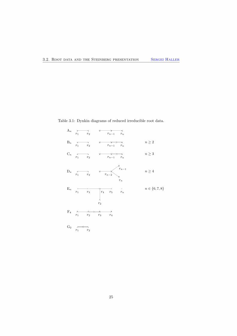
A Dynkin diagram D of a root datum R = (X,Φ, Y,Φ?) is a graph with
the vertex set labeled by the fundamental roots. Two distinct vertices ri and
rj are connected by 〈ri, r?j 〉〈rj , r?i 〉 edges. If the the number of edges between
ri and rj is at least 2, then one of the roots ri and rj is shorter than the
other. We indicate that by placing a less-than sign over the edges. The root
data are classified (see for example [6, Chapter VI]) and Table 3.1 shows all
Dynkin diagrams for a reduced irreducible root datum. The Dynkin diagram
of a reducible root datum is the disjoint union of the Dynkin diagrams of its
irreducible components.
Let G be a reductive linear algebraic group and fix a maximal torus T in G,
then a reduced root datumR = R(G,T ) can be constructed (see [32] for details).
Further, W =W (R) is isomorphic to NG(T )/T . By the Isomorphism Theorem
[32, 9.6.2], the group G is uniquely determined up to algebraic isomorphism by
its root datum and k.
24
3.2. Root data and the Steinberg presentation Sergei Haller
Table 3.1: Dynkin diagrams of reduced irreducible root data.
�� �� �� �� ��
r1 r2 rn−1 rn
An
�� �� �� �� ��
r1 r2 rn−1 rn
Bn n ≥ 2
�� �� �� �� ��
r1 r2 rn−1 rn
Cn n ≥ 3
�� �� �� ��
��
��r1 r2 rn−2
rn−1
rn
Dn n ≥ 4
� � � � �
�
r1
r2
r3 r4 r5 rn
En n ∈ {6, 7, 8}
� � � �
r1 r2 r3 r4
F4
� �
r1 r2
G2
25
Sergei Haller 3. Algebraic groups
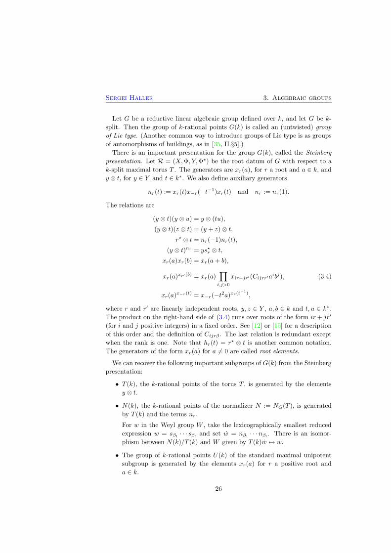
Let G be a reductive linear algebraic group defined over k, and let G be k-
split. Then the group of k-rational points G(k) is called an (untwisted) group
of Lie type. (Another common way to introduce groups of Lie type is as groups
of automorphisms of buildings, as in [35, II.§5].)There is an important presentation for the group G(k), called the Steinberg
presentation. Let R = (X,Φ, Y,Φ?) be the root datum of G with respect to a
k-split maximal torus T . The generators are xr(a), for r a root and a ∈ k, andy ⊗ t, for y ∈ Y and t ∈ k∗. We also define auxiliary generators
nr(t) := xr(t)x−r(−t−1)xr(t) and nr := nr(1).
The relations are
(y ⊗ t)(y ⊗ u) = y ⊗ (tu),
(y ⊗ t)(z ⊗ t) = (y + z)⊗ t,r? ⊗ t = nr(−1)nr(t),
(y ⊗ t)nr = ys?r ⊗ t,xr(a)xr(b) = xr(a+ b),
xr(a)xr′ (b) = xr(a)
∏
i,j>0
xir+jr′(Cijrr′aibj), (3.4)
xr(a)x−r(t) = x−r(−t2a)xr(t
−1),
where r and r′ are linearly independent roots, y, z ∈ Y , a, b ∈ k and t, u ∈ k∗.The product on the right-hand side of (3.4) runs over roots of the form ir+ jr′
(for i and j positive integers) in a fixed order. See [12] or [15] for a description
of this order and the definition of Cijrβ . The last relation is redundant except
when the rank is one. Note that hr(t) = r? ⊗ t is another common notation.
The generators of the form xr(a) for a 6= 0 are called root elements.
We can recover the following important subgroups of G(k) from the Steinberg
presentation:
• T (k), the k-rational points of the torus T , is generated by the elements
y ⊗ t.
• N(k), the k-rational points of the normalizer N := NG(T ), is generated
by T (k) and the terms nr.
For w in the Weyl group W , take the lexicographically smallest reduced
expression w = sβ1· · · sβl and set w = nβ1
· · ·nβl . There is an isomor-
phism between N(k)/T (k) and W given by T (k)w ↔ w.
• The group of k-rational points U(k) of the standard maximal unipotent
subgroup is generated by the elements xr(a) for r a positive root and
a ∈ k.
26
3.3. Automorphisms Sergei Haller
• Xr(k) := {xr(t) | t ∈ k} is the root subgroup of G(k) corresponding to the
root r ∈ Φ.
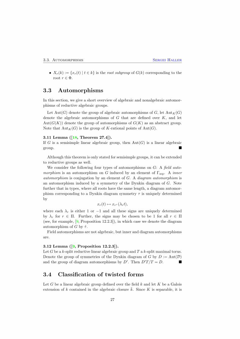
3.3 Automorphisms
In this section, we give a short overview of algebraic and nonalgebraic automor-
phisms of reductive algebraic groups.
Let Aut(G) denote the group of algebraic automorphisms of G, let AutK(G)
denote the algebraic automorphisms of G that are defined over K, and let
Aut(G(K)) denote the group of automorphisms of G(K) as an abstract group.
Note that AutK(G) is the group of K-rational points of Aut(G).
3.11 Lemma ([18, Theorem 27.4]).
If G is a semisimple linear algebraic group, then Aut(G) is a linear algebraic
group. ¥
Although this theorem is only stated for semisimple groups, it can be extended
to reductive groups as well.
We consider the following four types of automorphisms on G: A field auto-
morphism is an automorphism on G induced by an element of Γsep. A inner
automorphism is conjugation by an element of G. A diagram automorphism is
an automorphism induced by a symmetry of the Dynkin diagram of G. Note
further that in types, where all roots have the same length, a diagram automor-
phism corresponding to a Dynkin diagram symmetry τ is uniquely determined
by
xr(t) 7→ xrτ (λrt),
where each λr is either 1 or −1 and all these signs are uniquely determined
by λr for r ∈ Π. Further, the signs may be chosen to be 1 for all r ∈ Π
(see, for example, [9, Proposition 12.2.3]), in which case we denote the diagram
automorphism of G by τ .
Field automorphisms are not algebraic, but inner and diagram automorphisms
are.
3.12 Lemma ([9, Proposition 12.2.3]).
LetG be a k-split reductive linear algebraic group and T a k-split maximal torus.
Denote the group of symmetries of the Dynkin diagram of G by D := Aut(D)and the group of diagram automorphisms by D′. Then D′T/T = D. ¥
3.4 Classification of twisted forms
Let G be a linear algebraic group defined over the field k and let K be a Galois
extension of k contained in the algebraic closure k. Since K is separable, it is
27

Sergei Haller 3. Algebraic groups
contained in ksep. Let Γsep := Gal(ksep: k) and Γ := Gal(K: k). Then Γsep acts
continuously on G, as described in Section 3.1, and so Γsep also acts continuously
on Aut(G), the group of algebraic automorphisms of G as in (2.7) of Chapter 2.
Furthermore, actions of Γ on G(K) and on AutK(G) are induced by the actions
of Γsep on G and Aut(G). The first cohomology H1(
Γsep,Aut(G))
is called the
Galois cohomology of G. Note that H1(
Γsep, G)
and H1(
Γsep,Aut(G))
are often
denoted H1(
k,G)
and H1(
k,Aut(G))
in the literature.
Given α ∈ Z1(Γsep,Aut(G)), we define the ∗-action of Γsep on G with respect
to α as in Section 2.3:
g ∗ γ := gγαγ for γ ∈ Γ and g ∈ G,
and define Gα to be the group G with the ∗-action instead of the natural action
of Γsep on G. The group Gα is called the twisted form of G induced by α.
Although G and Gα are the same as abstract groups, they have different
groups of rational points. Let K be a Galois extension of k contained in k.
Then
Gα(K) = {g ∈ G | g ∗ γ = g for all γ ∈ Gal(ksep:K)}= {g ∈ G | gγαγ = g for all γ ∈ Gal(ksep:K)}.
(3.5)
Note that this agrees with the definition of G(K) in Section 3.1 if we take α to
be the trivial cocycle:
G1(K) = {g ∈ G | gγ1γ = g for all γ ∈ Gal(ksep:K)}= {g ∈ G | gγ = g for all γ ∈ Gal(ksep:K)} = G(K).
If G is reductive, then a group of rational points of Gα is called a twisted group
of Lie type.
The following proposition, when applied to L = ksep, states that groups of
rational points of two twisted forms are conjugate in Aut(G) if, and only if,
their cocycles are cohomologous. That is, twisted forms of G are classified by
H1(Γsep,Aut(G)).
3.13 Proposition.
Let G be a linear algebraic group defined over k. Let L be a Galois extension
of k contained in k and let K be a Galois extension of k contained in L. Let
Γ = Gal(L:K). Let α and β be in Z1(Γ,AutL(G)). The cocycles α and β are
cohomologous with respect to a ∈ AutL(G) (that is, β = α(a)) if, and only if,
Gα(K)a = Gβ(K).
Proof. First suppose we have a ∈ AutL(G) such that βγ = a−γαγa for all
γ ∈ Γ. Then g ∈ Gβ(K) if, and only if, ga−1 ∈ Gα(K), since
ga−1
=(
gγβγ)a−1
= gγ(a−γαγa)a
−1
= ga−1γαγ
28
3.5. Computation of the Galois cohomology Sergei Haller
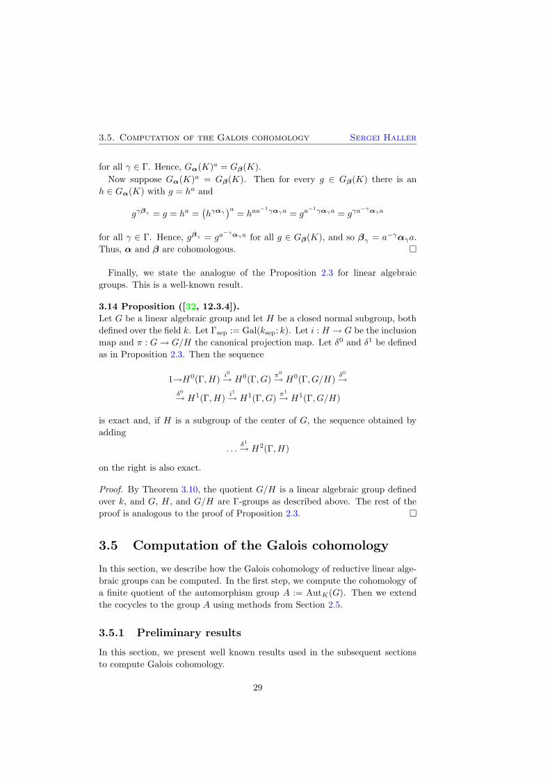
for all γ ∈ Γ. Hence, Gα(K)a = Gβ(K).
Now suppose Gα(K)a = Gβ(K). Then for every g ∈ Gβ(K) there is an
h ∈ Gα(K) with g = ha and
gγβγ = g = ha =(
hγαγ)a
= haa−1γαγa = ga
−1γαγa = gγa−γαγa
for all γ ∈ Γ. Hence, gβγ = ga−γαγa for all g ∈ Gβ(K), and so βγ = a−γαγa.
Thus, α and β are cohomologous. ¤
Finally, we state the analogue of the Proposition 2.3 for linear algebraic
groups. This is a well-known result.
3.14 Proposition ([32, 12.3.4]).
Let G be a linear algebraic group and let H be a closed normal subgroup, both
defined over the field k. Let Γsep := Gal(ksep: k). Let i : H → G be the inclusion
map and π : G→ G/H the canonical projection map. Let δ0 and δ1 be defined
as in Proposition 2.3. Then the sequence
1→H0(Γ, H)i0→ H0(Γ, G)
π0
→ H0(Γ, G/H)δ0→
δ0→ H1(Γ, H)i1→ H1(Γ, G)
π1
→ H1(Γ, G/H)
is exact and, if H is a subgroup of the center of G, the sequence obtained by
adding
. . .δ1→ H2(Γ, H)
on the right is also exact.
Proof. By Theorem 3.10, the quotient G/H is a linear algebraic group defined
over k, and G, H, and G/H are Γ-groups as described above. The rest of the
proof is analogous to the proof of Proposition 2.3. ¤
3.5 Computation of the Galois cohomology
In this section, we describe how the Galois cohomology of reductive linear alge-
braic groups can be computed. In the first step, we compute the cohomology of
a finite quotient of the automorphism group A := AutK(G). Then we extend
the cocycles to the group A using methods from Section 2.5.
3.5.1 Preliminary results
In this section, we present well known results used in the subsequent sections
to compute Galois cohomology.
29

Sergei Haller 3. Algebraic groups
3.15 Theorem (Springer’s Lemma, [30, Lemma III.6]).
Let C be a Cartan subgroup of a linear algebraic group G defined over k, and
let N := NG(C) be the normalizer of C in G. Let Γsep := Gal(ksep: k). The
canonical map H1(Γsep, N)→ H1(Γsep, G) is surjective. ¥
As in [32, 17.10.1], we say that a field k has cohomological dimension ≤ 1 if
there are no nontrivial central division algebras over k. Examples include finite
fields and the field of rational functions C(t).
3.16 Theorem ([30, Corollary 3 of Theorem III.3]).
Let G be a linear algebraic group defined over a perfect field k of dimension
≤ 1, let G◦ be its identity component, and let π : G → G/G◦ be the standard
projection. Then
π1 : H1(Γsep, G)→ H1(Γsep, G/G◦)
is bijective. ¥
The importance of this result for the computation of the Galois cohomology is
evident: it reduces the computation of the cohomology on G to the computation
of the cohomology on a finite group. An important special case of this theorem
is:
3.17 Theorem (Lang’s Theorem).
If G is a connected linear algebraic group defined over a finite field k, then
H1(Γsep, G) = 1. ¥
This theorem is often stated in the following, obviously equivalent, form:
3.18 Theorem (Lang’s Theorem).
Let G be a connected linear algebraic group defined over a finite field k with
|k| = q, and let F : G→ G be the field automorphism induced by
k → k, x 7→ xq.
Then the map
L : G→ G, h 7→ h−Fh
is surjective. ¥
3.5.2 Cohomology of DW
Let G be k-split reductive linear algebraic group. We use Springer’s Lemma 3.15
to compute Galois cohomology. First we compute the cohomology of Γsep on
DW , where W is the Weyl group and D is the symmetry group of the Dynkin
30
3.5. Computation of the Galois cohomology Sergei Haller
diagram of G. This is used to find the Galois cohomology of Aut(G) in Section
3.5.3.
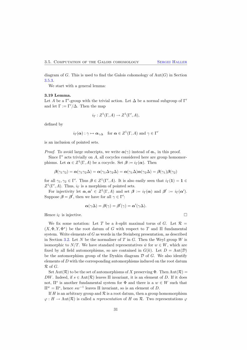
We start with a general lemma:
3.19 Lemma.
Let A be a Γ′-group with the trivial action. Let ∆ be a normal subgroup of Γ′
and let Γ := Γ′/∆. Then the map
iΓ : Z1(Γ, A)→ Z1(Γ′, A),
defined by
iΓ(α) : γ 7→ αγ∆ for α ∈ Z1(Γ, A) and γ ∈ Γ′
is an inclusion of pointed sets.
Proof. To avoid large subscripts, we write α(γ) instead of αγ in this proof.
Since Γ′ acts trivially on A, all cocycles considered here are group homomor-
phisms. Let α ∈ Z1(Γ, A) be a cocycle. Set β := iΓ(α). Then
β(γ1γ2) = α(γ1γ2∆) = α(γ1∆γ2∆) = α(γ1∆)α(γ2∆) = β(γ1)β(γ2)
for all γ1, γ2 ∈ Γ′. Thus β ∈ Z1(Γ′, A). It is also easily seen that iΓ(1) = 1 ∈Z1(Γ′, A). Thus, iΓ is a morphism of pointed sets.
For injectivity let α,α′ ∈ Z1(Γ, A) and set β := iΓ(α) and β′ := iΓ(α′).
Suppose β = β′, then we have for all γ ∈ Γ′:
α(γ∆) = β(γ) = β′(γ) = α′(γ∆).
Hence iΓ is injective. ¤
We fix some notation: Let T be a k-split maximal torus of G. Let R =
(X,Φ, Y,Φ?) be the root datum of G with respect to T and Π fundamental
system. Write elements of G as words in the Steinberg presentation, as described
in Section 3.2. Let N be the normaliser of T in G. Then the Weyl group W is
isomorphic to N/T . We have standard representatives w for w ∈W , which are
fixed by all field automorphisms, so are contained in G(k). Let D = Aut(D)be the automorphism group of the Dynkin diagram D of G. We also identify
elements ofD with the corresponding automorphisms induced on the root datum
R of G.
Set Aut(R) to be the set of automorphisms ofX preserving Φ. Then Aut(R) =
DW . Indeed, if s ∈ Aut(R) leaves Π invariant, it is an element of D. If it does
not, Πs is another fundamental system for Φ and there is a w ∈ W such that
Πw = Πs, hence sw−1 leaves Π invariant, so is an element of D.
IfH is an arbitrary group andR is a root datum, then a group homomorphism
ϕ : H → Aut(R) is called a representation of H on R. Two representations ϕ
31
Sergei Haller 3. Algebraic groups
and ψ of H on R are equivalent if there is an automorphism a ∈ Aut(R), such
that ϕ(h) = a−1ψ(h)a for all h ∈ H.
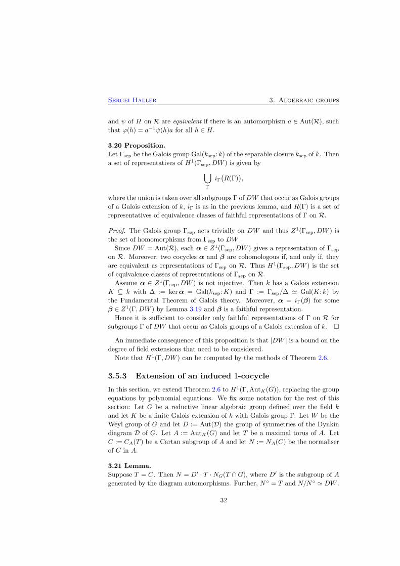
3.20 Proposition.
Let Γsep be the Galois group Gal(ksep: k) of the separable closure ksep of k. Then
a set of representatives of H1(Γsep, DW ) is given by
⋃
Γ
iΓ(
R(Γ))
,
where the union is taken over all subgroups Γ ofDW that occur as Galois groups
of a Galois extension of k, iΓ is as in the previous lemma, and R(Γ) is a set of
representatives of equivalence classes of faithful representations of Γ on R.
Proof. The Galois group Γsep acts trivially on DW and thus Z1(Γsep, DW ) is
the set of homomorphisms from Γsep to DW .
Since DW = Aut(R), each α ∈ Z1(Γsep, DW ) gives a representation of Γsepon R. Moreover, two cocycles α and β are cohomologous if, and only if, they
are equivalent as representations of Γsep on R. Thus H1(Γsep, DW ) is the set
of equivalence classes of representations of Γsep on R.
Assume α ∈ Z1(Γsep, DW ) is not injective. Then k has a Galois extension
K ⊆ k with ∆ := kerα = Gal(ksep:K) and Γ := Γsep/∆ ' Gal(K: k) by
the Fundamental Theorem of Galois theory. Moreover, α = iΓ(β) for some
β ∈ Z1(Γ, DW ) by Lemma 3.19 and β is a faithful representation.
Hence it is sufficient to consider only faithful representations of Γ on R for
subgroups Γ of DW that occur as Galois groups of a Galois extension of k. ¤
An immediate consequence of this proposition is that |DW | is a bound on the
degree of field extensions that need to be considered.
Note that H1(Γ, DW ) can be computed by the methods of Theorem 2.6.
3.5.3 Extension of an induced 1-cocycle
In this section, we extend Theorem 2.6 to H1(Γ,AutK(G)), replacing the group
equations by polynomial equations. We fix some notation for the rest of this
section: Let G be a reductive linear algebraic group defined over the field k
and let K be a finite Galois extension of k with Galois group Γ. Let W be the
Weyl group of G and let D := Aut(D) the group of symmetries of the Dynkin
diagram D of G. Let A := AutK(G) and let T be a maximal torus of A. Let
C := CA(T ) be a Cartan subgroup of A and let N := NA(C) be the normaliser
of C in A.
3.21 Lemma.
Suppose T = C. Then N = D′ · T ·NG(T ∩G), where D′ is the subgroup of A
generated by the diagram automorphisms. Further, N ◦ = T and N/N◦ ' DW .
32

3.5. Computation of the Galois cohomology Sergei Haller
Proof. N is the normaliser of the maximal torus T , hence consists of all diagonal
and diagram automorphisms, all conjugations by a Weyl or a torus element of
G, and their products. The connected component N ◦ consists of all diagonal
automorphisms. Finally,
N/N◦ = D′TNG(T ∩G)/T ' DW. ¤
Using the previous lemma and Section 3.5.2 we can compute the cohomology
on N/N◦. Next we have to extend the cocycles on N/N ◦ to cocycles on N .
This is done using methods of Section 2.5. Since the group N is in general
not finite, solving group equations directly is not feasible. We therefore replace
group equations over N by polynomial equations in several steps.
First we describe how to replace group equations over N by equations overW
and equations over T . Let α ∈ Z1(Γ, N/N◦). Recall the notation of Theorem
2.6: Let Γ = 〈γ1, . . . , γk | r1, . . . , r`〉. Since Γ is finite, we may take ri to be
words in γ1, . . . , γk not involving inverses. We fix a set {t(x) ∈ N | x ∈ N/N ◦}of coset representatives and introduce indeterminates b(γ1), . . . , b(γk) over N
◦.
Decompose the coset representatives t(αγi) = τγitγiwγi with τγi ∈ D, tγi ∈ T ,and wγi ∈ W . Decompose the indeterminates b(γi) = sγi vγi into new indeter-
minates sγi ∈ T and vγi ∈W . Then, for every relator r =∏mi=1 σi, the equation
m∏
i=1
(
(
t(ασi)b(σi))
∏mj=i+1 σj
)
= 1, (3.6)
corresponding to (2.8) and (2.9), is equivalent to equation
m∏
i=1
τσiwσivσi = 1 (3.7)
in DW with indeterminates vγi , and, for each given solution of (3.7), the equa-
tion
m∏
i=1
τσiwσi vσi
m∏
i=1
(twσiσi sσi)
Xi = 1 (3.8)
in T with indeterminates sγi , where
Xi = vσi
m∏
j=i+1
τσj wσj vσjσj .
To see this, we use the simple fact that xy = yxy for elements of a group and
that all τσi , wσi , and vσi commute with field automorphisms, we obtain (3.8)
from (3.6). Now
m∏
i=1
τσiwσi vσi =(
m∏
i=1
(twσiσi sσi)
Xi
)−1
∈ T
33

Sergei Haller 3. Algebraic groups
and thus
m∏
i=1
τσiwσivσi = 1.
Note that the right hand side of (3.8) is 1A = idG, and hence is conjugation by
an element from Z(G).
Let K[x1, . . . , x`] be a polynomial ring. A formal sum
p =n∑
i=0
ai
mi∏
j=1
yαijj ,
where n andmi are nonnegative integers, ai ∈ K, αij ∈ Γ, and yj ∈ {x1, . . . , x`},is called a (multivariate) polynomial over K with field automorphisms. The total
degree of p is max{m0, . . . ,mn}.Fix a solution vγi ∈W of (3.7). We now show that the group equation (3.8)
is equivalent to a polynomial equation with field automorphisms. The left hand
side of the equation
m∏
i=1
(twσiσi sσi)
Xi =(
m∏
i=1
τσiwσi vσi
)−1
is a torus element involving indeterminates. The right hand side is a known
torus element. Now we replace every indeterminate sσi over T by a d-tuple
of indeterminates over K, using the isomorphism T ' Gmd. Then the left
hand side becomes a d-tuple of polynomials with field automorphisms and the
equation is now equivalent to d polynomial equations with field automorphisms.
We now describe how to replace polynomials with a field automorphism by
ordinary polynomials. Let p be a polynomial with field automorphisms over K
in ` variables of total degree n. Let r := [K : k] and let (b1, . . . , br) be a basis
of K as a vector space over k. Substitute the formal sum∑r
j=1 bjxij for every
indeterminate xi of p, where xi1, . . . , xir are new indeterminates over the field
k. Then p becomes an ordinary polynomial s over K of the same total degree
n with r` variables. The map
(
aij ∈ k | i = 1, . . . , `, j = 1, . . . , r)
7→(
r∑
j=1
bjaij | i = 1, . . . , `)
is a bijection between the set of zeros of s in kr` and the set of zeros of p in K`.
A simpler approach is available when K is a finite field: Every γ ∈ Γ has the
form γ : x 7→ xqm
for some m, where q is the size of k. Substituting xqm
for xγ
provides an ordinary polynomial s′ of degree at most qmn in the same number
of variables. The zero sets of p and s′ are the same. The systems of polynomial
34
3.5. Computation of the Galois cohomology Sergei Haller
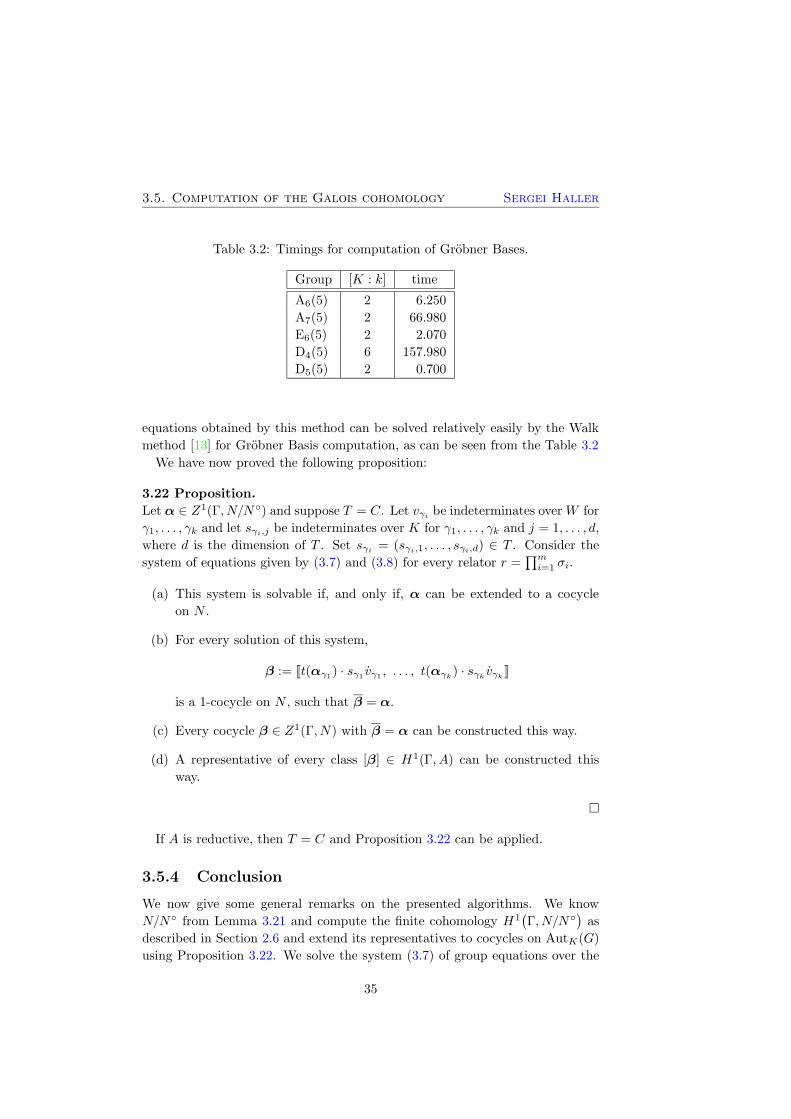
Table 3.2: Timings for computation of Grobner Bases.
Group [K : k] time
A6(5) 2 6.250
A7(5) 2 66.980
E6(5) 2 2.070
D4(5) 6 157.980
D5(5) 2 0.700
equations obtained by this method can be solved relatively easily by the Walk
method [13] for Grobner Basis computation, as can be seen from the Table 3.2
We have now proved the following proposition:
3.22 Proposition.
Let α ∈ Z1(Γ, N/N◦) and suppose T = C. Let vγi be indeterminates overW for
γ1, . . . , γk and let sγi,j be indeterminates over K for γ1, . . . , γk and j = 1, . . . , d,
where d is the dimension of T . Set sγi = (sγi,1, . . . , sγi,d) ∈ T . Consider the
system of equations given by (3.7) and (3.8) for every relator r =∏mi=1 σi.
(a) This system is solvable if, and only if, α can be extended to a cocycle
on N .
(b) For every solution of this system,
β := [[t(αγ1) · sγ1
vγ1, . . . , t(αγk) · sγk vγk ]]
is a 1-cocycle on N , such that β = α.
(c) Every cocycle β ∈ Z1(Γ, N) with β = α can be constructed this way.
(d) A representative of every class [β] ∈ H1(Γ, A) can be constructed this
way.
¤
If A is reductive, then T = C and Proposition 3.22 can be applied.
3.5.4 Conclusion
We now give some general remarks on the presented algorithms. We know
N/N◦ from Lemma 3.21 and compute the finite cohomology H1(
Γ, N/N◦)
as
described in Section 2.6 and extend its representatives to cocycles on AutK(G)
using Proposition 3.22. We solve the system (3.7) of group equations over the
35
Sergei Haller 3. Algebraic groups
Weyl group W and the corresponding system (3.8) of polynomial equations.
The polynomial equations are solved using methods for Grobner bases.
In general, all solutions of these systems of equations must be found. The
importance of Lemma 3.16 is that, whenever it holds, only one solution for each
system of equations is required.
We now discuss the cases where Lemma 3.16 cannot be applied. If the field
k is not perfect or not of dimension ≤ 1, then one of the following can happen:
1. The same cocycle from Z1(Γ, N/N◦) can be extended to (at least) two
non-cohomologous cocycles in Z1(Γ, N).
For example, A = Aut(SL2) ' PGL2 is connected, thus A/A◦ ' 1 and
there is only the trivial cocycle to extend. This lifts to the trivial cocycle
and to [[ch]] with h =(
1c
)
and c 6∈ NKk (K). (See Case 1 after the proof
of Proposition 4.12 in Section 4.5.1.)
2. Some cocycles in Z1(Γ, N/N◦) may have no extensions in Z1(Γ, N).
In this case Grobner basis methods would show that there are no solutions.
3.6 Example: GL1
In this section, we explicitly compute the cocycles and twisted forms of GL1.
See Section 4.5 for more examples. Recall the group G := Gm = GL1 defined
in the Section 3.1:
G = {(x, y) ∈ k2 | xy − 1 = 0}
with the multiplication (x1, y1) · (x2, y2) := (x1x2, y1y2).
For any Galois extension K of k contained in k, the group of rational points
is
G(K) = {(x, y) ∈ K2 | xy = 1}= {(x, y) ∈ K2 | y = x−1, x 6= 0} ' K∗
By considering polynomials in the variables x and y, which define group auto-
morphisms, we see that the group of algebraic automorphisms of G is
Aut(G) = 〈τ〉
with τ : (x, y) 7→ (y, x). Note that τ 2 = 1 and Aut(G) = AutK(G) for every K.
Now supposeK is an extension of degree 2 and set Γ := Gal(K: k) = 〈γ〉. Con-sider α ∈ Z1
(
Γ,AutK(G))
. Since every cocycle in Z1(
Γ,AutK(G))
is uniquely
determined by the image of γ, we have two cases:
Case 1: The trivial cocycle 1. Then G1(k) = G(k) ' k∗.
36
3.6. Example: GL1 Sergei Haller
Case 2: α = [[τ ]]. Then
Gα(k) = {g ∈ G(K) | gγαγ = g}= {(x, y) ∈ K2 | xy = 1 and (x, y)γτ = (x, y)}= {(x, y) ∈ K2 | xy = 1 and y = xγ}= {(x, y) ∈ K2 | xxγ = 1 and y = xγ}' {x ∈ K | xxγ = 1}.
That is, Gα(k) is the set of norm 1 elements of K. In other words, Gα(k)
is the subgroup of unitary matrices of GL1.
In the case k = Fq, we have K = Fq2 , γ : x 7→ xq,
G1(k) ' {x ∈ K | xq−1 = 1}, and
Gα(k) ' {x ∈ K | xq+1 = 1}.
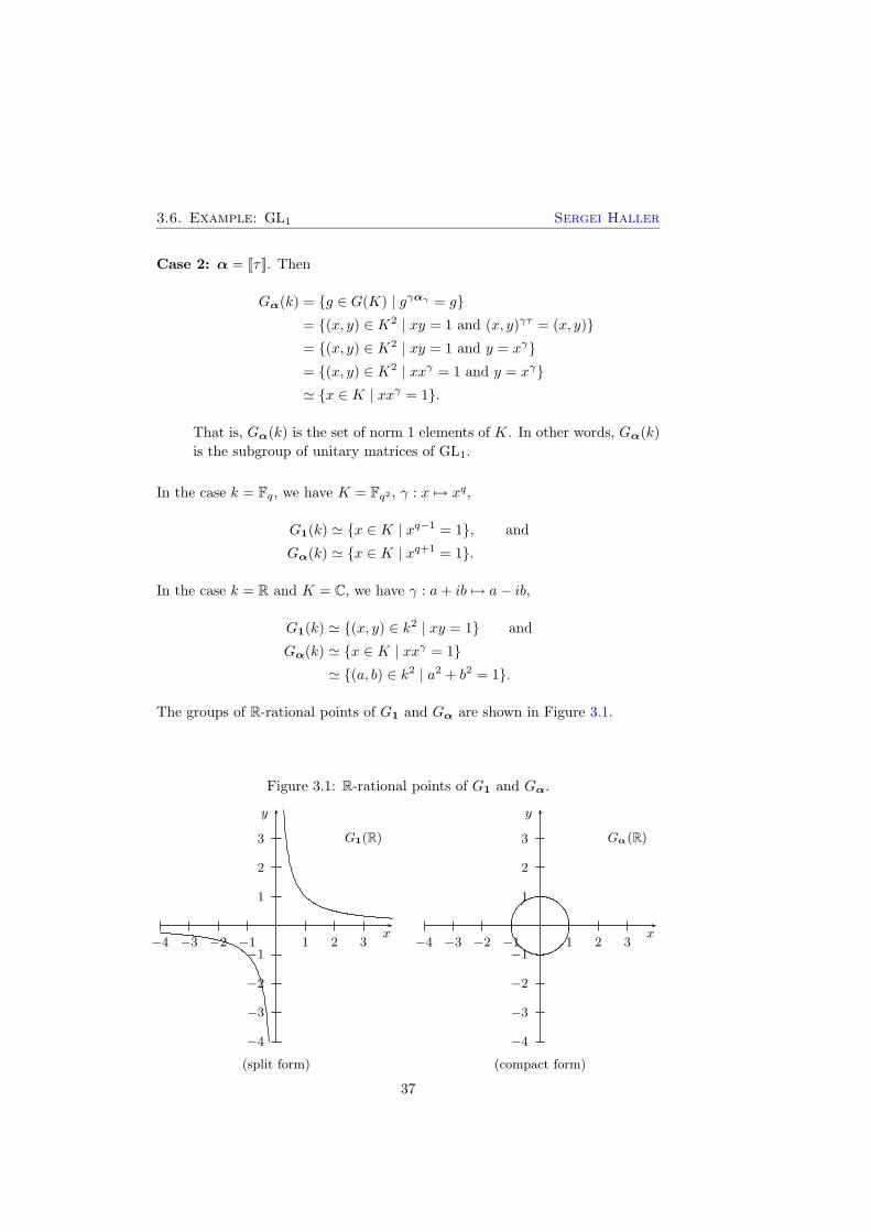
In the case k = R and K = C, we have γ : a+ ib 7→ a− ib,
G1(k) ' {(x, y) ∈ k2 | xy = 1} and
Gα(k) ' {x ∈ K | xxγ = 1}' {(a, b) ∈ k2 | a2 + b2 = 1}.
The groups of R-rational points of G1 and Gα are shown in Figure 3.1.
Figure 3.1: R-rational points of G1 and Gα.
1 2 3−1−2−3−4
1
2
3
−1
−2
−3
−4
x
y
G1(R)
(split form)
1 2 3−1−2−3−4
1
2
3
−1
−2
−3
−4
x
y
Gα(R)
(compact form)
37

Chapter 4
Twisted forms
In this chapter, we study twisted forms of reductive linear algebraic groups.
That is, we are given a reductive k-split linear algebraic group G defined over
a field k and a cocycle α ∈ H1(Γsep,Aut(G)), where Γsep := Gal(ksep: k) is the
Galois group of the separable closure of k. Using Springer’s Lemma 3.15, we can
assume that α stabilizes the standard k-split torus T . Then, as in Section 3.4,
the group of k-rational points of the twisted form Gα is
Gα(k) = {g ∈ G | gγαγ = g ∀γ ∈ Γsep}.
One can easily determine if a given element g ∈ G lies in Gα(k) or not. This is
not satisfactory for computing with Gα(k) however, since this definition gives
us no nontrivial elements to work with. To this end, we develop algorithms
for computing the normal subgroup Gα(k)† of Gα(k) generated by the root
elements. This also provides a presentation for Gα(k)†.
The quotient Gα(k)/Gα(k)† is called the Whitehead group, see for example
[38]. The determination of the Whitehead group is very hard in general. In [23,
Chapter 9], a general overview is given and, among other results, the Whitehead
group is proven to be trivial for algebraic number fields in all types other than2E6. We expect that our methods will be useful for determining the Whitehead
group.
Note that the methods presented here do not work for types 2B2,2G2 and
2F4,
since the map induced by the Dynkin diagram symmetry on the root lattice X
is not a linear map. We expect though, that our method will work if we replace
X, which is a Z-module spanned by the fundamental system Π, by a (Z+Z√2)-
module in cases 2B2 and 2F4 or a (Z + Z√3)-module in the case 2G2.
39
Sergei Haller 4. Twisted forms
4.1 Relative root system
Just as the Steinberg presentation for G(k) is based on a root datum, the pre-
sentation for Gα(k)† is based on a relative root system, which we describe in
this section. Our description is based on Satake [27] and Schattschneider [28].
First we make the connection between our notation and the notation in [28].
As usual, set A := Aut(G), Γ := Γsep = Gal(ksep: k), and let α ∈ Z1(Γ, NA(T ))
be a fixed cocycle. Let R = (X,Φ, Y,Φ?) be the root datum of G with funda-
mental system Π.
As shown in Section 3.5.2, H1(Γ, NA(T )/(NA(T ))◦) ' H1(Γ, DW ) and co-
cycles of DW are homomorphisms from Γ to DW . Since DW ' Aut(R), a
cocycle determines an action of Γ on R and thus a permutation action on the
root system Φ. This is the Γ-action in [28].
Let Oα(χ) denote the orbit of χ ∈ X under the Γ-action corresponding to
the cocycle α. By [28, (16)], either Oα(r) is contained in Φ+, or it is contained
in Φ−, or the sum of the roots of Oα(r) is zero. In the latter case, we have
∑
γ∈Γ
rαγ = 0,
which is equivalent to
∑
s∈Oα(r)
s = 0, (4.1)
since
∑
γ∈Γ
rαγ = m∑
s∈Oα(r)
s,
where m is the order of the stabilizer of r in Γ. Put
X0 := {χ ∈ X |∑
γ∈Γ
χαγ = 0} and (4.2)
XΓ := {χ ∈ X | χαγ = χ for all γ ∈ Γ} (4.3)
Let Φ0 := Φ ∩X0 and Π0 := Π ∩X0. Then, by [28, §1], X0 is a submodule of
X, Φ0 is a subsystem of Φ, and Π0 is a fundamental system of Φ0. Note that
Π0 is not necessarily a basis of X0 (a counterexample is given in Example 4.1).
Set X := X/X0 and let π : X → X be the standard projection. Then X is
a free Z-module and π is a homomorphism of modules. Let Ψ and ∆ be the
images under π of Φ \Φ0 and Π \Π0, respectively. Then Ψ is a root system and
∆ is a fundamental system of it. We call Ψ the relative root system and ∆ the
relative fundamental system. Note that Ψ need not be irreducible nor reduced
even if Φ is. The rank of the relative system is |∆| and is called the relative
40

4.1. Relative root system Sergei Haller
rank of Gα, whereas the rank |Π| of Φ is called the absolute rank. Let Ψ+ and
Ψ− denote the images under π of Φ+ \ Φ0 and Φ− \ Φ0. When X0 = X, the
relative root system is an empty set and the form is called anisotropic.
Let δ ∈ Ψ+ be a relative root. We fix a set of representatives of the orbits
Oα(r) with the property π(r) = δ and call this set Jδ Then, by [28, §2],
π−1(δ) =˙⋃
r∈Jδ
Oα(r) ⊆ Φ+ \ Φ0. (4.4)
We now construct an action of Γ on Π induced by the action on Φ. Remember
that αγ = τw for some τ ∈ D, w ∈W . Then γ acts on Π by
r 7→ rτ .
This is the [Γ]-action of [28]. The cocycle α and the corresponding twisted form
Gα are called inner if the [Γ]-action is trivial and outer otherwise. Let [O]α(r)
be the orbit of r ∈ Π under this action. Then, by [28, Proposition 3.5],
[O]α(r) = Π ∩ π−1(π(r)).
Computation of the actions of Γ on Φ and on Π, as well as the orbits of both
actions, is straightforward using the definitions, and is very fast. For example,
in type A20, the computation takes less than 2 seconds on a Pentium 1.6 GHz.
4.1 Example.
We illustrate this by a small example. Let Φ be a root system of type A3 and let
Π = {r1, r2, r3} be a fundamental root system of Φ with the Dynkin diagram:
�� �� ��
r1 r2 r3
Then the Weyl group W is generated by fundamental reflections s1, s2, and
s3. Let Γ = 〈γ〉 be of order 2. Choose the cocycle α = [[τs2]], where τ is the
non-trivial Dynkin diagram symmetry. Then
X0 = 〈r2, r1 − r3〉, Φ0 = {±r2}, and Π0 = {r2}.
The orbits of the actions of Γ on Φ and Π are
Oα(r1) = {r1, r2 + r3}, [O]α(r1) = {r1, r3},Oα(r2) = {r2,−r2}, [O]α(r2) = {r2},Oα(r3) = {r3, r1 + r2},
Oα(r1 + r2 + r3) = {r1 + r2 + r3},
together with the orbits lying entirely in Φ−, which are determined by negating
the orbits in Φ+. The relative root system is Ψ = {±δ1,±2δ1} with δ1 = π(r1).
41
Sergei Haller 4. Twisted forms
This is a root system of type BC1 with the fundamental system ∆ = {δ1}.Furthermore
π−1(δ1) = Oα(r1) ∪ Oα(r3) and π−1(2δ1) = Oα(r1 + r2 + r3).
Finally, we state several basic results that are used in Section 4.3
4.2 Lemma.
Let r and s be positive roots with r ∈ Φ+ \Φ0. If r+s ∈ Φ then r+s ∈ Φ+ \Φ0.
Proof. Every positive root is a unique linear combination of roots in Π with non-
negative coefficients. Since r 6∈ Φ0, the coefficient of at least one fundamental
root in Π\Π0 is positive in the linear combination of r. But then the coefficient
of this fundamental root in the linear combination of r + s is also positive. ¤
For the next lemma, recall that the only scalar multiples of a root r in a (not
necessarily reduced) root system are ± 12r, ±r and ±2r.
4.3 Lemma.
Let δ, ε ∈ Ψ+ and r ∈ π−1(δ), s ∈ π−1(ε). If ir + js ∈ Φ for positive integers i
and j, then iδ + jε ∈ Ψ+ and π(ir + js) = iδ + jε. In particular, if δ = ε, then
we must have i = j = 1 and π(r + s) = 2δ.
Proof. By the previous lemma, ir+js ∈ Φ+\Φ0, and, since π is a homomorphism
of Z-modules, we have π(ir + js) = iπ(r) + jπ(s) = iδ + jε ∈ Ψ+.
If δ = ε, then π(ir + js) = (i+ j)δ. This can only be a root in Ψ if i+ j = 2
since i and j are positive integers. ¤
Recall from Section 3.2 the notation for the maximal unipotent subgroup
U(K) of G(K) and the root subgroups.
4.4 Corollary.
Suppose δ ∈ Ψ+ but 2δ 6∈ Ψ and let r, s ∈ π−1(δ). Then [Xr, Xs] = 1.
Proof. By Equation (3.4) in Section 3.2, [xr(u), xs(v)] is a product of root el-
ements corresponding to roots in Φ+ that have the form ir + js for positive
integers i and j. But if ir+ js is a root for some positive integers i and j, then
i = j = 1 and π(r + s) = 2δ ∈ Ψ by Lemma 4.3, a contradiction to 2δ 6∈ Ψ. ¤
4.5 Corollary.
Suppose δ, 2δ ∈ Ψ+ and let r ∈ π−1(δ), s ∈ π−1(2δ). Then [Xr, Xs] = 1.
Proof. The commutator [xr(u), xs(v)] is a product of root elements correspond-
ing to roots in Φ+ that have the form ir+js with positive integers i and j. But if
ir+js is a root for some positive integers i and j, then π(ir+js) = (i+2j)δ ∈ Ψ
by Lemma 4.3 and i+ 2j ≥ 3, a contradiction. ¤
42
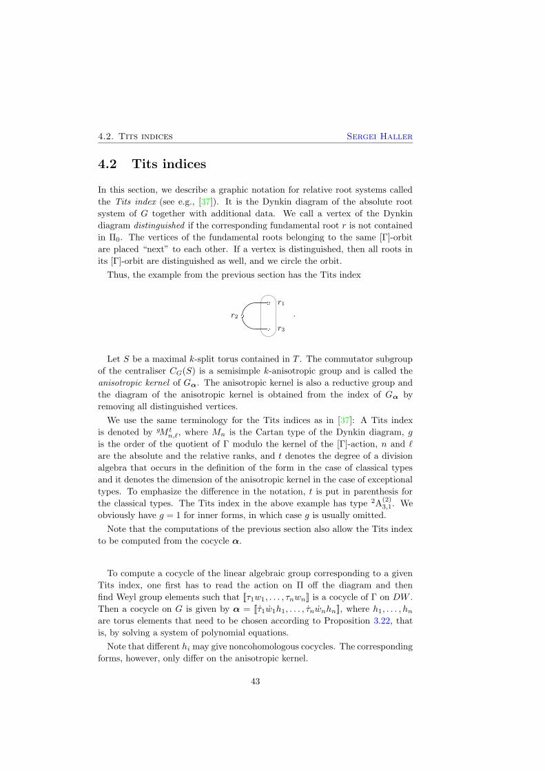
4.2. Tits indices Sergei Haller
4.2 Tits indices
In this section, we describe a graphic notation for relative root systems called
the Tits index (see e.g., [37]). It is the Dynkin diagram of the absolute root
system of G together with additional data. We call a vertex of the Dynkin
diagram distinguished if the corresponding fundamental root r is not contained
in Π0. The vertices of the fundamental roots belonging to the same [Γ]-orbit
are placed “next” to each other. If a vertex is distinguished, then all roots in
its [Γ]-orbit are distinguished as well, and we circle the orbit.
Thus, the example from the previous section has the Tits index
��
��
��
r1
r2
r3
.
Let S be a maximal k-split torus contained in T . The commutator subgroup
of the centraliser CG(S) is a semisimple k-anisotropic group and is called the
anisotropic kernel of Gα. The anisotropic kernel is also a reductive group and
the diagram of the anisotropic kernel is obtained from the index of Gα by
removing all distinguished vertices.
We use the same terminology for the Tits indices as in [37]: A Tits index
is denoted by gM tn,`, where Mn is the Cartan type of the Dynkin diagram, g
is the order of the quotient of Γ modulo the kernel of the [Γ]-action, n and `
are the absolute and the relative ranks, and t denotes the degree of a division
algebra that occurs in the definition of the form in the case of classical types
and it denotes the dimension of the anisotropic kernel in the case of exceptional
types. To emphasize the difference in the notation, t is put in parenthesis for
the classical types. The Tits index in the above example has type 2A(2)3,1. We
obviously have g = 1 for inner forms, in which case g is usually omitted.
Note that the computations of the previous section also allow the Tits index
to be computed from the cocycle α.
To compute a cocycle of the linear algebraic group corresponding to a given
Tits index, one first has to read the action on Π off the diagram and then
find Weyl group elements such that [[τ1w1, . . . , τnwn]] is a cocycle of Γ on DW .
Then a cocycle on G is given by α = [[τ1w1h1, . . . , τnwnhn]], where h1, . . . , hnare torus elements that need to be chosen according to Proposition 3.22, that
is, by solving a system of polynomial equations.
Note that different hi may give noncohomologous cocycles. The corresponding
forms, however, only differ on the anisotropic kernel.
43

Sergei Haller 4. Twisted forms
4.3 Root subgroups
The (standard) unipotent subgroup of Gα(k) is Uα(k) := U(K)∩Gα(k). We now
describe the root elements and root subgroups of Uα(k). Let γ ∈ Γ, let αγ = τn
for n ∈ N , and let w ∈W be the image of n under the natural homomorphism.
Then the image under γαγ of the root element xr(tr) for r ∈ Φ and tr ∈ K, is
xr(tr)γαγ = xrτw(λrγt
γr ),
where λrγ is a constant that depends on the root r and, for a fixed cocycle α,
on γ. Let δ ∈ Ψ be a relative root. Its preimages are, as described by (4.4),
π−1(δ) =˙⋃
r∈Jδ
Oα(r).
Symbolically construct a K-vector space Vδ with basis Jδ and denote by tr the
coefficient of r ∈ Jδ in the linear combination of t ∈ Vδ. For t ∈ Vδ set
uδ(t) =∏
r∈Jδ
∏
γ∈Γ
xr(tr)γαγ , (4.5)
where the whole product is taken in the ordering of the roots fixed for the uniquedecomposition of U in Section 3.2, and set
Uδ ={
uδ(t) | t ∈ Vδ}
. (4.6)
Then uδ(t)γαγ is the product of the same terms taken in a different order, since
(
xr(tr)γ′αγ′
)γαγ= xr(tr)
γ′γαγ
γ′αγ = xr(tr)
γ′γαγ′γ ,
and so uδ(t)γαγ = uδ(t)cγ(t). In other words, we set cγ(t) := uδ(t)
−1uδ(t)γαγ .
The following lemma provides a description of cγ(t). If δ, 2δ ∈ Ψ, set
Y2δ :=∏
r∈π−1(2δ)
Xr(K).
4.6 Lemma.
If 2δ 6∈ Ψ, then cγ(t) = 1 for all γ ∈ Γ. Otherwise cγ(t) ∈ Y2δ.
Proof. If 2δ is not a relative root, then all root elements in the product (4.5)
commute by Corollary 4.5.
If 2δ ∈ Ψ, then cγ(t) is a product of commutators of pairs of root elements
from the product (4.5). Let r, s ∈ π−1(δ) be two roots. By Lemma 4.3, the com-
mutator of root elements corresponding to these roots is a single root element
corresponding to the root r + s ∈ π−1(2δ). ¤
44

4.3. Root subgroups Sergei Haller
Let δ ∈ Ψ be a relative root. First we consider the case 2δ 6∈ Ψ. In this case
we define the relative root elements to be
xδ(t) := uδ(t) (4.7)
for t ∈ Vδ and the relative root subgroups Xδ := Uδ. Indeed, Xδ is an (abstract)
abelian group by Lemma 4.6 with relations
xδ(t) · xδ(s) = xδ(t+ s),
xδ(t)−1 = xδ(−t),
[
xδ(t), xδ(s)]
= 1
for t, s ∈ Vδ.Now consider the case where 2δ is also a relative root. Choose an arbitrary
u := uδ(t) and compute cγ(t) := u−1uγαγ for all γ ∈ Γ. We need a correction
term v ∈ U(K) such that
uv = (uv)γαγ = uγαγvγαγ = ucγ(t)vγαγ for all γ ∈ Γ,
which is equivalent to
cγ(t) = vv−γαγ for all γ ∈ Γ.
4.7 Lemma.
(a) For a given t, the map ρ : γ 7→ cγ(t) is a cocycle in Z1(Γ, Y2δ).
(b) There is a solution v for the system of equations
cγ(t) = vv−γαγ , γ ∈ Γ. (4.8)
Proof. To show that ρ is a cocycle, we compute
uδ(t)cγγ′(t) = uδ(t)γγ′αγγ′ = (uδ(t)
γαγ )γ′αγ′ = (uδ(t)cγ(t))
γ′αγ′
= uδ(t)cγ′(t)cγ(t)γ′αγ′ = uδ(t)cγ(t)
γ′αγ′ cγ′(t).
Hence, cγγ′(t) = cγ(t)γ′αγ′ cγ′(t). But Y2δ is unipotent, thus H
1(Γ, Y2δ) = 1 and
the constructed cocycle is cohomologous to the trivial one, that is, there is an
element v ∈ Y2δ such that cγ(t) = vv−γαγ for all γ ∈ Γ. ¤
A method to construct such a solution v for given elements cγ(t) is discussed
in the Section 4.4 below.
4.8 Lemma.
For given cγ(t), γ ∈ Γ, the set of solutions v ∈ Y2δ for (4.8) is the coset v1X2δ,
where v1 is any particular solution for this equation system.
45

Sergei Haller 4. Twisted forms
Proof. Let v be a solution of (4.8) and x ∈ X2δ, then vx ∈ Y2δ and
(vx)(vx)−γαγ = vxx−γαγv−γαγ = vxx−1v−γαγ = vv−γαγ = cγ(t)
for all γ ∈ Γ. Let on the other hand, v1 and v2 be two solutions for (4.8), then
v2v−γαγ
2 = cγ(t) = v1v−γαγ
1 ⇒ v−11 v2 = v−γαγ
1 vγαγ
2 = (v−11 v2)γαγ ,
for all γ ∈ Γ, thus v−11 v2 ∈ X2δ. ¤
Now we can define the relative root elements in the case δ ∈ Ψ with 2δ ∈ Ψ to
be
xδ(t) := uδ(t)v(t) (4.9)
for t ∈ Vδ, where v(t) ∈ Y2δ is an arbitrary fixed solution for (4.8). Define the
relative root subgroups to be
Xδ :=⟨
X2δ; xδ(t) | t ∈ Vδ⟩
.
Note that, by Lemma 4.8, the definition of Xδ does not depend on the choice
of the elements v(t) in (4.9).
4.9 Lemma.
(a) X2δ is a central subgroup of Xδ and Xδ =⟨
xδ(t) | t ∈ Vδ⟩
X2δ.
(b) Xδ ={
xδ(t)x2δ(s) | t ∈ Vδ, s ∈ V2δ}
Proof. (a) follows from the fact that elements xδ(t) and x2δ(s) commute for any
t ∈ Vδ, s ∈ V2δ by Corollary 4.5.
For (b), the inclusion of the right hand side in Xδ is trivial. For the other
inclusion, let xδ(t) = uδ(t)v(t) and xδ(s) = uδ(s)v(s) for t, s ∈ Vδ. Then
xδ(t)xδ(s) = uδ(t)v(t)uδ(s)v(s) = uδ(t)uδ(s)v(t)v(s)
= uδ(t+ s)y(t, s)v(t)v(s),
where y(t, s) is a product of root elements corresponding to roots in π−1(2δ),
and depends on t and s.
Now the element xδ(t)xδ(s) is fixed by γαγ and we have
uδ(t+ s)y(t, s)v(t)v(s) =(
uδ(t+ s)y(t, s)v(t)v(s))γαγ
= uδ(t+ s)γαγ(
y(t, s)v(t)v(s))γαγ
= uδ(t+ s)cγ(t+ s)(
y(t, s)v(t)v(s))γαγ
,
where cγ(t+ s) is as before and
cγ(t+ s) =(
y(t, s)v(t)v(s))(
y(t, s)v(t)v(s))−γαγ
.
46
4.4. Cohomology of unipotent subgroups Sergei Haller
Hence y(t, s)v(t)v(s) ∈ v(t+ s)X2δ by Lemma 4.8 and
xδ(t)xδ(s) = uδ(t+ s)y(t, s)v(t)v(s) ∈ xδ(t+ s)X2δ. ¤
Finally
xδ(t)xδ(s) ∈ xδ(t+ s)X2δ, (4.10)
xδ(t)−1 ∈ xδ(−t)X2δ, (4.11)
[
xδ(t), xδ(s)]
∈ X2δ. (4.12)
In particular, Xδ is nilpotent of nilpotency class 2. The exact relations between
relative root elements of this form can be easily computed inside the original
untwisted group of Lie type. For each group, we compute them for generic
relative root elements once, so we can use them for computations.
4.10 Proposition.
Uα(k) = 〈Xδ | δ ∈ Ψ+〉.
Proof. Let u ∈ Uα(k) be an arbitrary element. Write the unique decomposition
of u as a product of root elements. Let xr(v) be the first nontrivial root element
occurring in the decomposition, that is, r is the first root with coefficient v 6= 0.
Since xr(v) occurs in this product, xr(v)γαγ must also occur in the product
for each γ ∈ Γ, since u is fixed by γαγ . In particular, Oα(r) must be contained
in Φ+, hence δ := π(r) ∈ Ψ+. Now let t ∈ Vδ with tr = v and ts = 0
for r 6= s ∈ Jδ. Thus u = xδ(t)u′ and all root elements occurring in the
decomposition of u′ correspond to roots larger than r. Since the number of
roots is finite, u ∈ 〈Xδ | δ ∈ Ψ+〉 by induction. ¤
The relative root elements and relative root subgroups for negative relative
roots are defined in the similar way. Now we define a normal subgroup of Gα(k):
Gα(k)† := 〈Uα(k)g | g ∈ Gα(k)〉.
The quotient Gα(k)/Gα(k)† is called the Whitehead group. Its description is a
hard problem and is of interest for the study of Gα(k).
4.4 Cohomology of unipotent subgroups
Suppose we have a reductive algebraic group G defined over k and U is its
standard maximal unipotent subgroup. Let K be a Galois extension of k and
let Γ := Gal(K: k). In this section, we describe how to find an element v ∈ U(K)
with the property
cγ = vv−γαγ , for all γ ∈ Γ
47
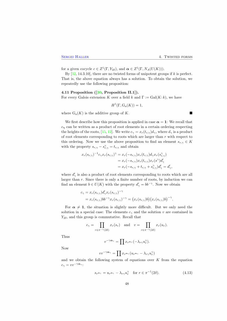
Sergei Haller 4. Twisted forms
for a given cocycle c ∈ Z1(Γ, Y2δ), and α ∈ Z1(Γ, NA(U(K))).
By [32, 14.3.10], there are no twisted forms of unipotent groups if k is perfect.
That is, the above equation always has a solution. To obtain the solution, we
repeatedly use the following proposition:
4.11 Proposition ([30, Proposition II.1]).
For every Galois extension K over a field k and Γ := Gal(K: k), we have
H1(Γ,Ga(K)) = 1,
where Ga(K) is the additive group of K. ¥
We first describe how this proposition is applied in case α = 1: We recall that
cγ can be written as a product of root elements in a certain ordering respecting
the heights of the roots, [15, 12]. We write cγ = xr(tr,γ)dγ , where dγ is a product
of root elements corresponding to roots which are larger than r with respect to
this ordering. Now we use the above proposition to find an element sr,γ ∈ K
with the property sr,γ − sγr,γ = tr,γ and obtain
xr(sr,γ)−1cγxr(sr,γ)
γ = xr(−sr,γ)xr(tr,γ)dγxr(sγr,γ)= xr(−sr,γ)xr(tr,γ)xr(sγ)d′γ= xr(−sr,γ + tr,γ + sγr,γ)d
′γ = d′γ ,
where d′γ is also a product of root elements corresponding to roots which are all
larger than r. Since there is only a finite number of roots, by induction we can
find an element b ∈ U(K) with the property d′γ = bb−γ . Now we obtain
cγ = xr(sr,γ)d′γxr(sr,γ)
−γ
= xr(sr,γ)bb−γxr(sr,γ)
−γ =(
xr(sr,γ)b)(
xr(sr,γ)b)−γ
.
For α 6= 1, the situation is slightly more difficult. But we only need the
solution in a special case: The elements cγ and the solution v are contained in
Y2δ, and this group is commutative. Recall that
cγ =∏
r∈π−1(2δ)
xr(sr) and v =∏
r∈π−1(2δ)
xr(ur).
Thus
v−γαγ =∏
xrαγ (−λrγuγr ).Now
vv−γαγ =∏
xrαγ (urαγ − λrγuγr )and we obtain the following system of equations over K from the equation
cγ = vv−γαγ :
srαγ = urαγ − λrγuγr for r ∈ π−1(2δ). (4.13)
48
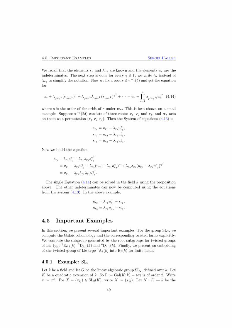
4.5. Important Examples Sergei Haller
We recall that the elements sr and λrγ are known and the elements ur are the
indeterminates. The next step is done for every γ ∈ Γ, we write λr instead of
λrγ to simplify the notation. Now we fix a root r ∈ π−1(δ) and get the equation
for
sr + λrα
−1γ
(srα
−1γ
)γ + λrα
−1γλrα
−2γ
(srα
−2γ
)γ2
+ · · · = ur −o∏
i=1
λr(α
−iγ )u
γo
r (4.14)
where o is the order of the orbit of r under αγ . This is best shown on a small
example: Suppose π−1(2δ) consists of three roots: r1, r2 and r3, and αγ acts
on them as a permutation (r1, r2, r3). Then the System of equations (4.13) is
sr1 = ur1 − λr3uγr3 ,sr2 = ur2 − λr1uγr1 ,sr3 = ur3 − λr2uγr2 .
Now we build the equation
sr1 + λr3sγr3 + λr3λr2s
γ2
r2
= ur1 − λr3uγr3 + λr3(ur3 − λr2uγr2)γ + λr3λr2(ur2 − λr1uγr1)
γ2
= ur1 − λr3λr2λr1uγ3
r1 .
The single Equation (4.14) can be solved in the field k using the proposition
above. The other indeterminates can now be computed using the equations
from the system (4.13). In the above example,
ur2 = λr1uγr1 − sr2 ,
ur3 = λr2uγr2 − sr3 .
4.5 Important Examples
In this section, we present several important examples. For the group SL2, we
compute the Galois cohomology and the corresponding twisted forms explicitly.
We compute the subgroup generated by the root subgroups for twisted groups
of Lie type 2E6,1(k),3D4,1(k) and
6D4,1(k). Finally, we present an embedding
of the twisted group of Lie type 2A7(k) into E7(k) for finite fields.
4.5.1 Example: SL2
Let k be a field and let G be the linear algebraic group SL2, defined over k. Let
K be a quadratic extension of k. So Γ := Gal(K: k) = 〈σ〉 is of order 2. Write
x := xσ. For X = (xij) ∈ SL2(K), write X := (xij). Let N : K → k be the
49

Sergei Haller 4. Twisted forms
norm map defined by x 7→ xx. We denote by cg the conjugation automorphism
x 7→ xg induced by g ∈ GL2(K).
Let A := AutK(G) ' PGL2(K). Then Γ acts on A as in Section 2.3: ϕσ =
σ−1ϕσ = σϕσ for ϕ ∈ A. But now ϕ = cg for some g ∈ GL2(K), so
ϕσ = cσg = cg.
4.12 Proposition.
Let α ∈ Z1(Γ, A). Then ασ = ch for some h ∈ GL2(K) with the following
properties:
1. hh = xI2 for some x ∈ k∗; and
2. either h =(
0 1c 0
)
for c ∈ k∗ (in this case is x = c); or h =(
a bc 1
)
for
a, b, c ∈ K with a = −cc−1 = −bb−1 (in this case aa = 1 and x = cb+ 1).
Proof. Since α is a cocycle, ασ ∈ AutK(G) and ασ = ch for some h ∈ GL2(K).
Thus, idG = ασ2 = ασσ ·ασ = chh. Hence, hh = xI2 for some x ∈ K∗. Now let
h =(
a bc d
)
.
Case d = 0: Then b 6= 0 and we can assume b = 1 (otherwise replace h by
b−1h). Now xI2 = hh =(
aa+c aca c
)
. Thus a = 0 and x = c = c ∈ k∗.
Case d 6= 0: Here we can assume d = 1 (otherwise replace h by d−1h). Now
xI2 = hh =(
aa+bc ab+bca+c cb+1
)
. And it follows that c = −ca and b = −ab.Further, x = cb+ 1. ¤
We wish to determine which cocycles α = [[ch]] ∈ Z1(Γ, A) are cohomologous
to the trivial cocycle and find the intertwining elements for them. A cocycle α
is cohomologous to 1 if, and only if, ασ = ϕ−σϕ for some ϕ = cg ∈ A and this
is true if, and only if, there is a y ∈ K∗ with ygh = g. Now the problem is to
find such g and y. Set g := (gij).
Case 1: h =(
1c
)
, c ∈ k∗.Then g = ygh =
( ycg12 yg11ycg22 yg21
)
. Thus we get five equations:
g11 = ycg12, g12 = yg11, det g 6= 0,
g21 = ycg22, g22 = yg21,
and these are equivalent to
N(y) = c−1, g12 = yg11, det g 6= 0,
g22 = yg21.
Hence α is cohomologous to the trivial cocycle if, and only if, c is in
the image of the norm map. If it is, ϕ = cg with g =( 1 y
i yi
)
, where
50
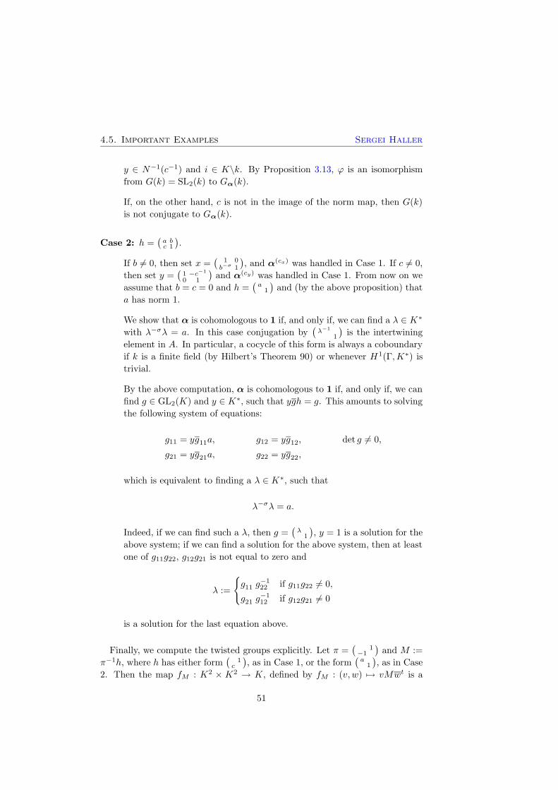
4.5. Important Examples Sergei Haller
y ∈ N−1(c−1) and i ∈ K\k. By Proposition 3.13, ϕ is an isomorphism
from G(k) = SL2(k) to Gα(k).
If, on the other hand, c is not in the image of the norm map, then G(k)
is not conjugate to Gα(k).
Case 2: h =(
a bc 1
)
.
If b 6= 0, then set x =(
1 0b−σ 1
)
, and α(cx) was handled in Case 1. If c 6= 0,
then set y =(
1 −c−1
0 1
)
and α(cy) was handled in Case 1. From now on we
assume that b = c = 0 and h =(
a1
)
and (by the above proposition) that
a has norm 1.
We show that α is cohomologous to 1 if, and only if, we can find a λ ∈ K∗
with λ−σλ = a. In this case conjugation by(
λ−1
1
)
is the intertwining
element in A. In particular, a cocycle of this form is always a coboundary
if k is a finite field (by Hilbert’s Theorem 90) or whenever H1(Γ,K∗) is
trivial.
By the above computation, α is cohomologous to 1 if, and only if, we can
find g ∈ GL2(K) and y ∈ K∗, such that ygh = g. This amounts to solving
the following system of equations:
g11 = yg11a, g12 = yg12, det g 6= 0,
g21 = yg21a, g22 = yg22,
which is equivalent to finding a λ ∈ K∗, such that
λ−σλ = a.
Indeed, if we can find such a λ, then g =(
λ1
)
, y = 1 is a solution for the
above system; if we can find a solution for the above system, then at least
one of g11g22, g12g21 is not equal to zero and
λ :=
{
g11 g−122 if g11g22 6= 0,
g21 g−112 if g12g21 6= 0
is a solution for the last equation above.
Finally, we compute the twisted groups explicitly. Let π =(
1−1
)
and M :=
π−1h, where h has either form(
1c
)
, as in Case 1, or the form(
a1
)
, as in Case
2. Then the map fM : K2 × K2 → K, defined by fM : (v, w) 7→ vMwt is a
51
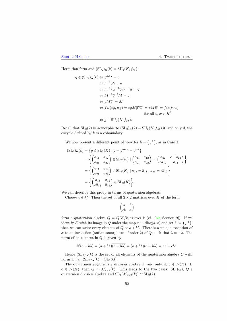
Sergei Haller 4. Twisted forms
Hermitian form and (SL2)α(k) = SU2(K, fM ):
g ∈ (SL2)α(k)⇔ gσασ = g
⇔ h−1gh = g
⇔ h−1ππ−1gππ−1h = g
⇔M−1g−tM = g
⇔ gMgt =M
⇔ fM (vg, wg) = vgMgtwt = vMwt = fM (v, w)
for all v, w ∈ K2
⇔ g ∈ SU2(K, fM ).
Recall that SL2(k) is isomorphic to (SL2)α(k) = SU2(K, fM ) if, and only if, the
cocycle defined by h is a coboundary.
We now present a different point of view for h =(
1c
)
, as in Case 1:
(SL2)α(k) ={
g ∈ SL2(K) | g = gσασ = gσh}
=
{(
a11 a12a21 a22
)
∈ SL2(K) |(
a11 a12a21 a22
)
=
(
a22 c−1a21ca12 a11
)}
=
{(
a11 a12a21 a22
)
∈ SL2(K) | a22 = a11, a21 = ca12
}
=
{(
a11 a12ca12 a11
)
∈ SL2(K)
}
.
We can describe this group in terms of quaternion algebras:
Choose c ∈ k∗. Then the set of all 2× 2 matrices over K of the form(
a b
cb a
)
form a quaternion algebra Q = Q(K/k, c) over k (cf. [39, Section 9]). If we
identify K with its image in Q under the map a 7→ diag(a, a) and set λ :=(
1c
)
,
then we can write every element of Q as a+ bλ. There is a unique extension of
σ to an involution (antiautomorphism of order 2) of Q, such that λ = −λ. Thenorm of an element in Q is given by
N(a+ bλ) = (a+ bλ)(a+ bλ) = (a+ bλ)(a− bλ) = aa− cbb.
Hence (SL2)α(k) is the set of all elements of the quaternion algebra Q with
norm 1, i.e., (SL2)α(k) = SL1(Q).
The quaternion algebra is a division algebra if, and only if, c 6∈ N(K). If
c ∈ N(K), then Q ' M2×2(k). This leads to the two cases: SL1(Q), Q a
quaternion division algebra and SL1(M2×2(k)) ' SL2(k).
52

4.5. Important Examples Sergei Haller
4.5.2 A twisted form of E6 of rank 1: 2E35
6,1(k)
Let R = (X,Φ, Y,Φ?) be the adjoint root datum of type E6 and G(k) = E6(k)
be given by the Steinberg presentation. Let Π be a fundamental system with
the following Dynkin diagram D:
�� �� �� �� ��
��
r1
r2
r3 r4 r5 r6
Denote the highest root by r∗. We also use the notation acdefb
for the root
ar1 + br2 + · · · + fr6. In this section, we compute relative root elements and
root subgroups for the twisted group of Lie type corresponding to the Tits index2E356,1(k):
�� ��
��
��
��
��
r1
r2
r3
r4
r5 r6
This form is known not to exist over finite fields, over p-adic fields, or over R.
There are number fields k over which this form exists (see for example Selbach
[29]). We compute 2E356,1(k)† as a subgroup of E6(K), where K is a quadratic
extension of k. Denote by γ the non-trivial automorphism in Γ := Gal(K: k).
The cocycle
First we compute a cocycle of Γ on AutK(G) defining a twisted form corre-
sponding to the above index. As described in Section 4.2, this amounts to find
a Weyl group element w, such that τw has the needed action on Φ and Π, where
τ is the non-trivial symmetry of D. Recall the notation τ from Section 3.3. Next
we have to find a torus element h, such that
α := [[τ wh]]
is a cocycle.
We know from the Tits index that Π0 = {r1, r3, . . . , r6} and Φ0 is the sub-
system of Φ spanned by Π0 of type A5. The Weyl element w = w0(Φ0) has the
required properties for the Γ-action on Φ. The orbits of Γ on Φ, that sum up
to 0 and those contained in Φ+ are given by
Oα(r) = {r,−r} if r ∈ Φ0,
Oα(r∗) = {r∗},Oα(r) = {r, r∗ − r} if r ∈ Φ+ \ Φ0 and r 6= r∗.
53

Sergei Haller 4. Twisted forms
The relative root system Ψ = {±δ,±2δ} has type BC1 with
π−1(δ) =˙⋃
r∈Jδ
Oα(r),
π−1(2δ) = Oα(r∗)
where Jδ = { 000001, 00100
1, 01100
1, 00110
1, 11100
1}. We denote the elements of Jδ by
β1, . . . , β5 and set βi := βτwi−5 for i = 6, . . . , 10.
Now that we have the required actions of Γ on Φ and Π, we have to choose
a torus element h =∏6i=1 hαi(si), where si ∈ k∗. For α to be a cocycle, γαγ
must have order 2, which is true if, and only if,
s22s23s34s25s6 = −1.
Hence s1 is determined by s2, . . . , s6:
s1 = −(s22s23s34s25s6)−1.
By construction, σ leaves the subgroup A5(K) := 〈Xr(K) | r ∈ Φ0〉 of G(K)
invariant and the restriction of σ to this subgroup is also an algebraic automor-
phism defining a cocycle.
Further we assume the existence of s1, s2, s3, . . . , s6 ∈ k∗, such that the group
(A5)α(k) is an anisotropic twisted group of Lie type. Basically, this means that
the standard representation of the torus element∏
i∈I hαi(si) in SL6(K) defines
an anisotropic unitary form q on K6 and (A5)α(k) ' SU6(k, q).
Relative root elements
We use methods from Section 4.3. By (4.5) and (4.7), we have
x2δ(t) = u2δ(t) =∏
xr∗(tr∗)γαγ = xr∗(tr∗ − tγr∗).
For the root δ, we first compute
uδ(t) =∏
r∈Jδ
∏
xr(tr)γαγ
and c(t) can be computed, but we omit the details. To compute v(t), we intro-
duce constants
cr =
6∏
i=1
s〈r,r?i 〉i ∈ k∗.
Then for t ∈ K:
xr(t)αγ = xrτw(Nr,rτw · cr · t),
xr∗(t)αγ = xr∗(cr∗ · t).
54

4.5. Important Examples Sergei Haller
In characteristic not 2, we introduce a k-valued bilinear form g : Vδ × Vδ → k:
g(t, u) :=
10∑
i=1
cβitβiuγβi.
Then a solution v(t) for the equation (4.8) is
v(t) = − 12g(t, t)
and the relative root element is
xδ(t) = uδ(t)v(t).
4.5.3 The groups 3D4,1(k) and 6D4,1(k)
Let R = (X,Φ, Y,Φ?) be the adjoint root datum of type D4. In this section, we
compute the root elements of the twisted groups of Lie type corresponding to
the Tits diagrams 3D4,1 and 6D4,1, both corresponding to the following figure:
��
��
��
��r2
r1
r3
r4
Both these groups were of recent interest, see for example [24].
We start by computing the relative root systems and the root orbits under
the actions of Γ on Φ and Π as described in Section 4.1. We use the notation
of that section and denote the highest root by r∗.
The group of all its symmetries of the Dynkin diagram is D = 〈τ3, τ2〉, whereτ3 = (r1, r3, r4) and τ2 = (r3, r4). Recall the notation τ from Section 3.3.
Type 3D4,1
If Γ has order 3, then there is no cocycle in Z1(Γ, DW ) with the properties
Oα(r2) ⊂ Φ+,∑
γ∈Γ
rγi = 0 for i = 1, 3, 4.
The smallest possible field extension, for which such a cocycle exists, has cyclic
Galois group of order 6, which we consider in the following construction. Let
Γ = 〈γ〉.
55
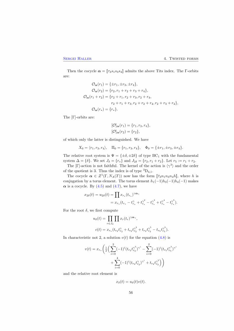
Sergei Haller 4. Twisted forms
Then the cocycle α = [[τ3s1s3s4]] admits the above Tits index. The Γ-orbits
are:
Oα(r1) = {±r1,±r3,±r4},Oα(r2) = {r2, r1 + r2 + r3 + r4},
Oα(r1 + r2) = {r2 + r1, r2 + r3, r2 + r4,
r2 + r1 + r3, r2 + r2 + r4, r2 + r3 + r4},Oα(r∗) = {r∗}.
The [Γ]-orbits are:
[O]α(r1) = {r1, r3, r4},[O]α(r2) = {r2},
of which only the latter is distinguished. We have
X0 = 〈r1, r3, r4〉, Π0 = {r1, r3, r4}, Φ0 = {±r1,±r3,±r4}.
The relative root system is Ψ = {±δ,±2δ} of type BC1 with the fundamental
system ∆ = {δ}. We set Jδ = {r∗} and J2δ = {r2, r1 + r2}. Let r5 := r1 + r2.
The [Γ]-action is not faithful. The kernel of the action is 〈γ3〉 and the order
of the quotient is 3. Thus the index is of type 3D4,1.
The cocycle α ∈ Z1(Γ, NA(T )) now has the form [[τ3n1n3n4h]], where h is
conjugation by a torus element. The torus element h1(−1)h3(−1)h4(−1) makes
α is a cocycle. By (4.5) and (4.7), we have
x2δ(t) = u2δ(t) =∏
xr∗(tr∗)γαγ
= xr∗(tr∗ − tγr∗ + tγ2
r∗ − tγ3
r∗ + tγ4
r∗ − tγ5
r∗ ).
For the root δ, we first compute
uδ(t) =∏
r∈Jδ
∏
xr(tr)γαγ ,
c(t) = xr∗(tr2tγr2 + tr2t
γ3
r2 + tr2tγ5
r2 − tr5tγ3
r5 ).
In characteristic not 2, a solution v(t) for the equation (4.8) is
v(t) = xr∗
(
12
(
2∑
i=0
(−1)i(tr2tγ3
r2 )γi −
2∑
i=0
(−1)i(tr5tγ3
r5 )γi
+
4∑
i=0
(−1)i(tr2tγr2)γi + tr2t
γ5
r2
)
)
and the relative root element is
xδ(t) = uδ(t)v(t).
56
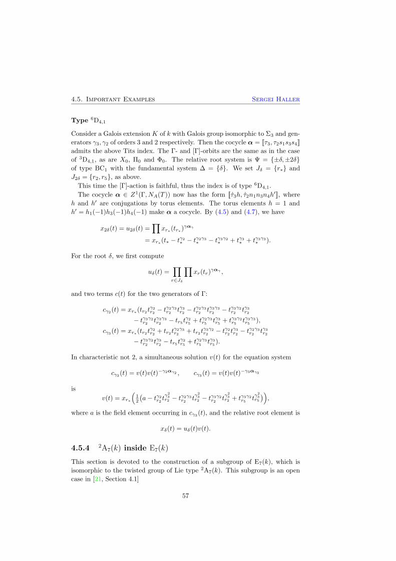
4.5. Important Examples Sergei Haller
Type 6D4,1
Consider a Galois extension K of k with Galois group isomorphic to Σ3 and gen-
erators γ3, γ2 of orders 3 and 2 respectively. Then the cocycle α = [[τ3, τ2s1s3s4]]
admits the above Tits index. The Γ- and [Γ]-orbits are the same as in the case
of 3D4,1, as are X0, Π0 and Φ0. The relative root system is Ψ = {±δ,±2δ}of type BC1 with the fundamental system ∆ = {δ}. We set Jδ = {r∗} and
J2δ = {r2, r5}, as above.This time the [Γ]-action is faithful, thus the index is of type 6D4,1.
The cocycle α ∈ Z1(Γ, NA(T )) now has the form [[τ3h, τ2n1n3n4h′]], where
h and h′ are conjugations by torus elements. The torus elements h = 1 and
h′ = h1(−1)h3(−1)h4(−1) make α a cocycle. By (4.5) and (4.7), we have
x2δ(t) = u2δ(t) =∏
xr∗(tr∗)γαγ
= xr∗(t∗ − tγ2∗ − tγ2γ3
∗ − tγ3γ2∗ + tγ3
∗ + tγ3γ3∗ ).
For the root δ, we first compute
uδ(t) =∏
r∈Jδ
∏
xr(tr)γαγ ,
and two terms c(t) for the two generators of Γ:
cγ2(t) = xr∗(tr2t
γ2r2 − t
γ2γ3r2 tγ3
r2 − tγ2γ3r2 tγ3γ3
r2 − tγ3γ2r2 tγ3
r2
− tγ3γ2r2 tγ3γ3
r2 − tr5tγ2r5 + tγ2γ3
r5 tγ3r5 + tγ3γ2
r5 tγ3γ3r5 ),
cγ3(t) = xr∗(tr2t
γ2r2 + tr2t
γ2γ3r2 + tr2t
γ3γ2r2 − tγ2
r2 tγ3r2 − t
γ2γ3r2 tγ3
r2
− tγ3γ2r2 tγ3
r2 − tr5tγ2r5 + tγ2γ3
r5 tγ3r5 ).
In characteristic not 2, a simultaneous solution v(t) for the equation system
cγ2(t) = v(t)v(t)−γ2αγ2 , cγ3
(t) = v(t)v(t)−γ3αγ3
is
v(t) = xr∗
(
12
(
a− tγ2r2 t
γ23r2 − tγ2γ3
r2 tγ23r2 − tγ3γ2
r2 tγ23r2 + tγ3γ2
r5 tγ23r5
)
)
,
where a is the field element occurring in cγ3(t), and the relative root element is
xδ(t) = uδ(t)v(t).
4.5.4 2A7(k) inside E7(k)
This section is devoted to the construction of a subgroup of E7(k), which is
isomorphic to the twisted group of Lie type 2A7(k). This subgroup is an open
case in [21, Section 4.1]
57
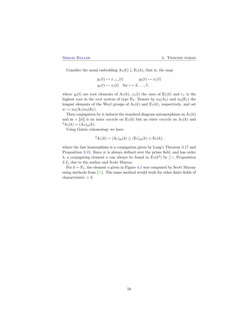
Sergei Haller 4. Twisted forms
Consider the usual embedding A7(k) ⊆ E7(k), that is, the map
y1(t) 7→ x−r∗(t) y2(t) 7→ x1(t)
yi(t) 7→ xi(t) for i = 3, . . . , 7,
where yi(t) are root elements of A7(k), xi(t) the ones of E7(k) and r∗ is the
highest root in the root system of type E7. Denote by w0(A7) and w0(E7) the
longest elements of the Weyl groups of A7(k) and E7(k), respectively, and set
w := w0(A7)w0(E7).
Then conjugation by w induces the standard diagram automorphism on A7(k)
and α = [[w]] is an inner cocycle on E7(k) but an outer cocycle on A7(k) and2A7(k) = (A7)α(k).
Using Galois cohomology we have
2A7(k) = (A7)α(k) ⊆ (E7)α(k) ' E7(k),
where the last isomorphism is a conjugation given by Lang’s Theorem 3.17 and
Proposition 3.13. Since w is always defined over the prime field, and has order
4, a conjugating element a can always be found in E7(k4) by [11, Proposition
2.1], due to the author and Scott Murray.
For k = F5, the element a given in Figure 4.1 was computed by Scott Murray
using methods from [11]. The same method would work for other finite fields of
characteristic > 3.
58
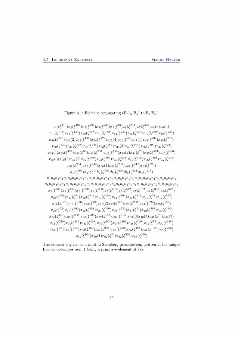
4.5. Important Examples Sergei Haller
Figure 4.1: Element conjugating (E7)α(F5) to E7(F5).
x1(ξ416)x2(ξ
494)x3(ξ234)x4(ξ
286)x5(ξ78)x6(ξ
234)x7(ξ598)x8(3)x9(3)
x10(ξ104)x11(ξ
130)x12(ξ598)x13(ξ
182)x14(ξ234)x15(ξ
520)x17(ξ260)x18(ξ
234)
x20(ξ286)x22(2)x23(ξ
130)x24(ξ572)x25(4)x26(ξ
26)x27(1)x28(ξ234)x29(ξ
286)
x30(ξ130)x31(ξ
338)x32(ξ546)x33(ξ
182)x34(3)x35(ξ104)x36(ξ
390)x37(ξ572)
x38(1)x39(ξ494)x40(ξ
52)x41(ξ260)x42(ξ
598)x43(2)x44(ξ78)x45(ξ
494)x46(ξ286)
x48(3)x50(2)x51(1)x52(ξ390)x53(ξ
390)x54(ξ208)x55(ξ
416)x56(ξ494)x57(ξ
494)
x58(ξ234)x59(ξ
442)x60(1)x61(ξ208)x62(ξ
442)x63(ξ520)
h1(ξ260)h2(ξ
91)h3(ξ390)h4(ξ
260)h5(ξ221)h7(ξ
117)
n1n2n3n1n4n2n3n1n4n3n5n4n2n3n1n4n3n5n4n2n6n5n4n2n3n1n4n3n5n4n2
n6n5n4n3n1n7n6n5n4n2n3n1n4n3n5n4n2n6n5n4n3n1n7n6n5n4n2n3n4n5n6n7
x1(ξ494)x2(ξ
104)x3(ξ390)x4(ξ
208)x5(ξ234)x6(ξ
572)x7(ξ182)x8(ξ
338)x9(ξ572)
x10(ξ286)x11(ξ
52)x12(ξ546)x13(ξ
234)x14(ξ104)x15(ξ
546)x16(ξ78)x17(ξ
572)
x18(ξ130)x19(ξ
416)x20(ξ78)x21(2)x22(ξ
572)x23(ξ260)x24(ξ
520)x25(ξ182)
x26(ξ52)x27(ξ
390)x28(ξ208)x29(ξ
390)x30(ξ520)x31(ξ
52)x32(ξ364)x33(ξ
234)
x34(ξ338)x35(ξ
208)x36(ξ208)x37(ξ
182)x38(ξ104)x39(3)x40(4)x41(ξ
78)x42(3)
x43(ξ520)x44(ξ
182)x45(ξ338)x46(ξ
104)x47(ξ494)x48(ξ
260)x49(ξ78)x50(ξ
338)
x51(ξ78)x52(ξ
494)x53(ξ182)x54(ξ
260)x55(ξ260)x56(ξ
494)x57(ξ130)x58(ξ
260)
x59(ξ104)x60(1)x61(ξ
26)x62(ξ520)x63(ξ
260)
The element is given as a word in Steinberg presentation, written in the uniqueBruhat decomposition, ξ being a primitive element of F54 .
59
Chapter 5
Maximal tori and Sylow
subgroups
Let G be a reductive algebraic group defined over the field k and Γsep :=
Gal(ksep: k). A twisted torus of G is a twisted form Tα of the standard maxi-
mal torus T ⊆ G, where α ∈ Z1(Γsep, NAut(G)(T )). In this section, we give a
classification of all twisted tori of G using the methods of the previous chap-
ters. In case k is finite, we compute them explicitly. For this computation,
we need a set of conjugacy class representatives of the Weyl group of Gβ for
β ∈ Z1(Γsep, NAut(G)(T )). The conjugacy classes of Weyl groups are known
(see, for example, [22, 8]) and, in [14], algorithms for their computation are
described.
5.1 Twisted maximal tori
In this section, we provide a classification of all twisted tori ofG(k) and, for finite
fields k, we compute them explicitly. It is well known that all the maximal tori
of G are conjugate in G (Theorem 3.6). We are interested the G(k)-conjugacy
classes of the groups of k-rational points of maximal k-tori of G.
We use the cohomology of Γsep on DW , where D is the automorphism group
of the Dynkin diagram and W the Weyl group of G. Therefore, we retain
the notation of Section 3.5.2: Let T be a maximal k-split torus of G and let
R = (X,Φ, Y,Φ?) be the root datum of G with respect to T . Write elements of
G as words in the Steinberg generators, as described in Section 3.2. Let N be
the normaliser of T in G. The Weyl group W is isomorphic to N/T . We have
standard representatives w ∈ N for each w ∈ W , which are invariant under all
field automorphisms, thus contained in G(k). LetD be the automorphism group
of the Dynkin diagram D of G and identify D with the group of automorphisms
induced on the root datum R of G. Then Aut(R) = DW .
61
Sergei Haller 5. Maximal tori and Sylow subgroups
First we consider cocycles that have values in NAut(G)(T ). Remember that,
for a twisted form Gβ of G, the cocycle β can be assumed to have values in
NAut(G)(T ) by Springer’s Lemma 3.15. Thus, Tβ ≤ Gβ is a maximal torus of
Gβ and all its twisted forms are obtained by cocycles with values in NAut(G)(T ).
That is, we obtain in one step not only all twisted tori of G, but also all twisted
tori of all twisted forms of G.
Note that in the following proposition we do not make any restrictions on the
choice of k.
5.1 Proposition.
The set of representatives of NAut(G)(T )-conjugacy classes of twisted tori of G
is⋃
Γ
{ Tα | α ∈ iΓ(
R(Γ))
},
where the union is taken over all subgroups of DW that occur as Galois groups
of a Galois extension of k, iΓ is as in Lemma 3.19, and R(Γ) is a set of repre-
sentatives of equivalence classes of faithful representations of Γ on R.
Proof. The NAut(G)(T )-conjugacy classes of twisted tori are classified by ele-
ments of H1(Γsep, NAut(G)(T )).
Let N be the normaliser of T in G andW = N/T be the Weyl group. If n1, n2are two elements of N with n1T = n2T , then conjugation by n1 and by n2 give
the same automorphism of T . Thus, NAut(G)(T )/CAut(G)(T ) ' D′N/T ' DW ,
where D′ is the group of diagram automorphisms.
Now Γsep acts trivially on NAut(G)(T ), and so on DW , and thus
H1(Γsep, NAut(G)(T )) = H1(Γsep, DW ).
The rest follows from Proposition 3.20. ¤
Note that for non-isomorphic field extensions K1 and K2 of k that have iso-
morphic Galois groups Γ := Gal(K1: k) ' Gal(K2: k), and for ρ ∈ iΓ(R(Γ)), thegroups of rational points Tρ(K1) and Tρ(K2) are not isomorphic in general.
5.2 Corollary.
If k is finite, a set of representatives of the NAut(G)(T )-conjugacy classes of
twisted tori of G is given by
{Tα | α = [[w]], w ∈ R},
where R is a set of conjugacy class representatives of elements of DW .
Proof. For finite fields, the finite Galois groups are always cyclic. Let Γ = 〈γ〉be a cyclic group and α,β : Γ → DW two faithful representations of Γ on
62

5.2. Rational maximal tori Sergei Haller
R. Then o(αγ) = o(γ) and α,β are equivalent if, and only if, αγ and βγ are
conjugate in DW .
Thus, equivalence classes of faithful representations of Γ correspond to con-
jugacy classes of elements of DW of order |Γ|. And
⋃
Γ
{ Tα | α ∈ R(Γ) } = { Tα | α = [[w]], w ∈ R },
where R is a set of conjugacy class representatives of elements of DW . ¤
If k is finite, we also write Tw instead of T[[w]] for w ∈ DW .
5.2 Rational maximal tori
In this section, we describe the rational maximal tori of all twisted and un-
twisted forms Gβ(k) of G(k) and, over finite fields, we classify and compute
them explicitly.
5.3 Lemma.
Let α,β ∈ iΓ(
R(Γ))
, with the notation of Proposition 5.1. These cocycles
naturally embed in Z1(Γ,AutK(G)). If they are cohomologous as cocycles in
Z1(Γ,AutK(G)), then Tα(k) is conjugate in AutK(G) to the group of rational
points of a maximal torus of Gβ(k).
Proof. Suppose, α is cohomologous to β. That is, there is an a ∈ AutK(G)
such that αγ = a−γβγa for all γ ∈ Γ. Then
Tα(k)a−1 ⊆ Gα(k)
a−1
= Gβ(k)
by Proposition 3.13. ¤
If a ∈ G(k) is as in this proof, then Tα(k)a−1
is called a rational maximal torus
of Gβ(k).
An important special case is given by the following lemma, which, together
with Corollary 5.2, provides a classification of all rational maximal tori of twisted
and untwisted finite groups of Lie type.
Denote the Weyl group of Gβ by Wβ.
5.4 Lemma.
Let k be finite. Define cocycles β = [[τ ]] for τ ∈ D and α = [[τw]] for some
w ∈ Wβ as in Corollary 5.2. Then Tα(k) is conjugate in Gβ(k) to a rational
maximal torus of Gβ(k).
63
Sergei Haller 5. Maximal tori and Sylow subgroups
Proof. We apply Lang’s theorem to the group Gβ. By Lang’s theorem, applied
to the group Gβ, [[w]] is a coboundary in Z1(Γ, Gβ); thus
w = a−γβγ · 1 · a = τ−1a−γτa
and the intertwining element a is contained in Gβ(k). Now α = [[τw]] is coho-
mologous to β as elements of Z1(Γ,Aut(G)) with the same intertwining element
a. The result now follows from the previous lemma. ¤
Note that, the lemma remains true with k replaced by a finite extension of k.
An algorithm for the construction of the conjugator a is given in [11].
Now we summarise Corollary 5.2 and Lemma 5.4 as
5.5 Corollary.
Let k be a finite field and let β = [[τ ]] for some τ ∈ D. A set of representatives
of the Gβ(k)-conjugacy classes of groups of k-rational points of maximal tori of
Gβ is given by
{T awα (k) | α = [[τw]], w ∈ R},
where R is a set of conjugacy class representatives in Wβ , and aw is the inter-
twining element from the previous lemma, i.e.,
w = a−γτw aw.
5.3 Generators of twisted tori
In this section, we compute the generators of twisted tori explicitly in the case
k is finite. Let the notation be as in the previous section. Denote by ` the
semisimple rank of G. Note that methods from this and the next section do not
apply for twisted groups of types 2B2,2G2 and 2F4, since the map induced by
the Dynkin diagram symmetry on the root lattice is not a linear map.
5.6 Theorem.
Let w be an element of DW with order r. Let q := |k|, and let K be the field
extension of k of degree r in k. Let Γ := Gal(K: k) = 〈γ〉. Set m := |K∗| =qr − 1. Let M be the matrix of the action of w? on Y and let ξ be a primitive
element of K. Then
Tw(k) =⟨
(ξa1 , . . . , ξa`) | (a1, . . . , a`) ∈ B⟩
,
where B is a generating set of the fixed-point space in Z`m of qM , interpreted
as a matrix over Zm.
64
5.4. Computing orders of the maximal tori Sergei Haller
Proof. Let t ∈ T (K). Then, in the notation of Section 3.2,
t =∏
i=1
α?i ⊗ xi
with xi ∈ K∗. Moreover, for all i = 1, . . . , ` we have xi = ξai for some ai ∈ Zm.
By [12, 5.2]
tw =∏
j=1
α?j ⊗(
∏
i=1
xMij
i
)
=∏
j=1
α?j ⊗(
∏
i=1
ξaiMij
)
.
Since γ : x 7→ xq in our case,
tγw =∏
j=1
α?j ⊗(
∏
i=1
ξaiqMij
)
=∏
j=1
α?j ⊗ ξ
(
∑
i=1
aiqMij
)
.
Thus,
tγw = t ⇐⇒∑
i=1
aiqMij = aj for all j = 1, . . . , `
⇐⇒ (a1, . . . , a`)qM = (a1, . . . , a`).
That is,
Tw(k) ={
(ξa1 , . . . , ξa`) | (a1, . . . , a`) ∈ Z`m, (a1, . . . , a`)(qM − I) = 0}
. (5.1)
¤
Note that for different primitive elements of K this fixed-point space is the
same: For, let ξ, ζ be two primitive elements in K and t = (ξa1 , . . . , ξa`) =
(ζb1 , . . . , ζb`). Then ζ = ξc for some invertible c ∈ Zm and the exponent vector
(a1, . . . , a`) is an eigenvector of qM to the eigenvalue 1 if, and only if, the
exponent vector (b1, . . . , b`) is one as well:
(b1, . . . , b`)qM = c(a1, . . . , a`)qM = c(a1, . . . , a`) = (b1, . . . , b`).
5.4 Computing orders of the maximal tori
Let the notation be as in the previous sections. The maximal tori of G are given
by Corollary 5.2 and Theorem 5.6. The maximal tori are abelian groups which
can be written as a direct product of cyclic subgroups. Given the type of the
root datum of G and an element w ∈ DW , we now compute the orders of the
cyclic factors of Tw(k), as polynomials in q.
65

Sergei Haller 5. Maximal tori and Sylow subgroups
This is done in essentially the same way as in the proof of the Theorem
5.6. We interpret q, the order of k, as an indeterminate, so the Equation (5.1)
becomes{
(ξa1 , . . . , ξa`)∣
∣
∣(a1, . . . , a`) ∈
(
Z[q]/(qr − 1))`,
(a1, . . . , a`)(qM − I) = 0}
.
NowB := qM−I is a matrix over Z[q]/(qr−1) and the order of the solution space
of the equation XB = 0 is exactly the order of Tw(k), where X ∈(
Z[q]/(qr −1))`. We can view B as a matrix over Q[q]/(qr − 1). Using Magma we obtain
the Smith form S of B by elementary matrix transformations. The order of the
solution space of XS = 0 is the same as the order of Tw(k). The order of the
solution space of XS = 0 can now be read from the diagonal entries of S: Set
si :=
{
qr − 1 if Sii = 0,
Sii otherwise
and obtain
Tw(k) =∏
i=1
Csi ,
where si is the i-th diagonal entry of S and Ca is a cyclic group of order a.
A priori, the Smith form S is a diagonal matrix over Q[q]/(qr − 1). Every
diagonal entry has the form si = fi/gi with fi ∈ Z[q]/(qr − 1) and gi ∈ Z. First
we replace every zero on the diagonal by qr−1 and then multiply the last row by∏`−1i=1 g
−1i and all other rows by gi, thus preserving the determinant and making
all but the last entry have integral coefficients. But the determinant of the
matrix obtained is the same as the determinant of B, which is the characteristic
polynomial of the matrixM , hence a polynomial with integral coefficients. Now
the last entry also has integral coefficients. All diagonal entries of the matrix
obtained are factors of the characteristic polynomial.
The results for exceptional types are given in Appendix A.
Raghunathan [25] uses similar techniques to describe the twisted tori, al-
though only in the quasisplit case.
5.7 Example (A1 = SL2).
G(k) = SL2(k), k = GF (q), W = 〈w〉 ' C2. Standard torus:
T (k) = T1(k) = {( a
a−1
)
| a ∈ k∗} ' k∗ ' Cq−1.
Twisted torus: o(w) = 2, thus K = GF (q2), Γ = Gal(K: k) = 〈γ〉. Now
Tw(k) = {t ∈ T (K) | tγw = t} = {(
aaγ)
∈ SL2(K)}' {a ∈ K∗ | aaγ = 1} ' Cq+1.
66

5.5. Computation of Sylow p-subgroups Sergei Haller
Examples for types G2, F4, E6, E7, E8,2A5,
3D4 and 2E6 are stated in
Appendix A.
5.5 Computation of Sylow p-subgroups
We recall that G is a reductive linear algebraic group defined over the field k,
which we assume to be finite of order q in this section. The aim of this section is
to construct a “standard” Sylow p-subgroup of G(k) for every prime p dividing
the order of G(k).
If the prime p is the characteristic of the field k, the maximal unipotent sub-
groups are precisely the Sylow p-subgroups and have order qN , where N is the
number of positive roots of the underlying root system. Using the Steinberg pre-
sentation, we already have a standard choice of a maximal unipotent subgroup:
the subgroup U(k).
From now on we assume that p is different from the characteristic of k. Let
S be a Sylow p-subgroup of G(k). Then S is nilpotent and each element of S is
semisimple. Hence, by Corollary [31, 5.19],
S ≤ NG(k)(Tw(k)) (5.2)
for some (not necessarily unique) w ∈W and we have
NG(k)(Tw(k))/Tw(k) ' CW (w)
and
|NG(k)(Tw(k))| = |Tw(k)| · |CW (w)|.
In case p - |CW (w)|, we have S ≤ Tw(k) and we call the prime p nice.
5.8 Algorithm.
Note that when p is nice, steps 3 and 8 can be omitted.
0. Let pm := |G(k)|p. (A formula for |G(k)| can be found, e.g., in [9])
1. Let R be a set of conjugacy class representatives of W .
Using [14, Algorithm H] by Geck and Pfeiffer, each representative has the
shortest length among all elements of its conjugacy class.
2. Replace R by the set
{
w ∈ R∣
∣ pm divides |NG(k)(Tw(k))|}
. (5.2’)
(Otherwise a contradiction to (5.2).)
67
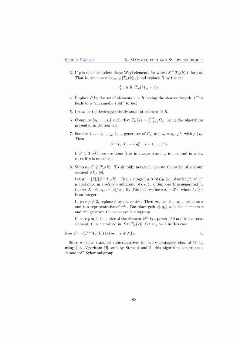
Sergei Haller 5. Maximal tori and Sylow subgroups
3. If p is not nice, select those Weyl elements for which S ∩ Tw(k) is largest.That is, set u := maxw∈R{|Tw(k)|p} and replace R by the set
{
w ∈ R∣
∣|Tw(k)|p = u}
.
4. Replace R by the set of elements w ∈ R having the shortest length. (This
leads to a “maximally split” torus.)
5. Let w be the lexicographically smallest element of R.
6. Compute [s1, . . . , s`] such that Tw(k) =∏`i=1 Csi using the algorithms
presented in Section 5.4.
7. For i = 1, . . . , `, let gi be a generator of Csi and si = oi · pxi with p - oi.
Then
S ∩ Tw(k) = 〈 goii | i = 1, . . . , ` 〉.
If S ⊆ Tw(k), we are done (this is always true if p is nice and in a few
cases if p is not nice).
8. Suppose S 6⊆ Tw(k). To simplify notation, denote the order of a group
element g by |g|.Let po = |S|/|S ∩ Tw(k)|. Find a subgroup H of CW (w) of order po, which
is contained in a p-Sylow subgroup of CW (w). Suppose H is generated by
the set X. Set qx := |x|/|x|. By Tits [36], we have qx = 2`x , where `x ≥ 0
is an integer.
In case p 6= 2, replace x by mx := xqx . Then mx has the same order as x
and is a representative of xqx . But since gcd(|x|, qx) = 1, the elements x
and xqx generate the same cyclic subgroup.
In case p = 2, the order of the element x|x| is a power of 2 and it is a torus
element, thus contained in |S ∩ Tw(k)|. Set mx := x in this case.
Now S = 〈(S ∩ Tw(k)) ∪ {mx | x ∈ X}〉. ¤
Since we have standard representatives for every conjugacy class of W by
using [14, Algorithm H], and by Steps 4 and 5, this algorithm constructs a
“standard” Sylow subgroup.
68
Appendix A
Decomposition of orders of
maximal tori
In this appendix we present the tables of the decomposed orders of maximal
tori of twisted and untwisted reductive linear algebraic groups defined over
finite fields. Note that the types 2B2,2G2 and 2F4 are not included here, since
the permutation on Φ induced by the Dynkin diagram symmetry is not a linear
map and thus our method doesn’t work.
A.1 How to read the tables
Each row contains the orders o1, . . . , on of cyclic components of the torus Tw(q) 'Co1 × · · · × Con , where w ∈ W is given as a word in the simple reflections. For
example, in the last line of Table A.1, the Weyl element is
w := s1s2s1s2s1s2,
where W = 〈s1, s2〉 is the Weyl group of G2(q) and
Tw(q) ' Cq+1 × Cq+1.
The generators of the Weyl groups are ordered as shown in the following
Dynkin diagrams. The numbering of fundamental roots is as in Table 3.1.
Computation of the decompositions of all exceptional types takes a total of
about 8 seconds on an Intel Pentium III 1.6GHz processor.
69

Sergei Haller A. Decomposition of orders of maximal tori
A.2 Tables
Table A.1: Maximal tori in G2(q)
Orders Weyl word
q − 1, q − 1
q2 − 1 1
q2 − 1 2
q2 − q + 1 12
q2 + q + 1 1212
q + 1, q + 1 121212
Table A.2: Maximal tori in F4(q)
Orders Weyl word
q − 1, q − 1, q − 1, q − 1
q − 1, q − 1, q2 − 1 1
q − 1, q − 1, q2 − 1 3
q − 1, q3 − 1 12
q2 − 1, q2 − 1 13
q − 1, q3 − q2 + q − 1 23
q − 1, q3 − 1 34
q4 − q3 + q − 1 123
q4 + q3 − q − 1 124
q4 + q3 − q − 1 134
q4 − q3 + q − 1 234
q4 − q2 + 1 1234
q2 − 1, q − 1, q + 1 2323
q2 + 1, q2 − 1 12323
q2 + 1, q2 − 1 23234
q4 + 1 123234
q2 − q + 1, q2 − q + 1 12132343
q + 1, q + 1, q2 − 1 121321323
q + 1, q + 1, q2 − 1 232343234
q + 1, q3 + 1 1213213234
q + 1, q3 + 1 1232343234
q2 + 1, q2 + 1 121321343234
q + 1, q3 + q2 + q + 1 12132132343234
q2 + q + 1, q2 + q + 1 1213213432132343
Continued on next page
70

A.2. Tables Sergei Haller
Table A.2 – continued from previous page
Orders Weyl word
q + 1, q + 1, q + 1, q + 1 121321323432132343213234
Table A.3: Maximal tori in E6(q)
Orders Weyl word
q − 1, q − 1, q − 1, q − 1, q − 1, q − 1
q − 1, q − 1, q − 1, q − 1, q2 − 1 1
q − 1, q − 1, q2 − 1, q2 − 1 12
q − 1, q − 1, q − 1, q3 − 1 13
q − 1, q − 1, q4 + q3 − q − 1 123
q2 − 1, q2 − 1, q2 − 1 125
q − 1, q − 1, q4 − 1 134
q − 1, q5 − 1 1234
q2 − 1, q4 + q3 − q − 1 1235
q2 − 1, q4 − 1 1245
q3 − 1, q − 1, q2 + q + 1 1356
q2 − 1, q4 − q3 + q − 1 2345
q6 − q4 + q2 − 1 12345
q6 + q5 − q − 1 12346
q2 + q + 1, q4 + q3 − q − 1 12356
q2 + q + 1, q4 − q3 + q − 1 13456
q6 + q5 − q3 + q + 1 123456
q3 − q2 + q − 1, q3 − q2 + q − 1 234254
q6 − q5 + q4 − q2 + q − 1 1234254
q6 + q3 + 1 12342546
q2 − q + 1, q4 + q2 + 1 123142345465
q + 1, q + 1, q2 − 1, q2 − 1 234234542345
q + 1, q + 1, q4 − 1 1234234542345
q + 1, q5 + q4 + q3 + q2 + q + 1 12342345423456
q2 + q + 1, q2 + q + 1, q2 + q + 1 123142314542314565423456
Table A.4: Maximal tori in E7(q)
Orders Weyl word
q − 1, q − 1, q − 1, q − 1, q − 1, q − 1, q − 1
q − 1, q − 1, q − 1, q − 1, q − 1, q2 − 1 1
q − 1, q − 1, q − 1, q2 − 1, q2 − 1 12
Continued on next page
71
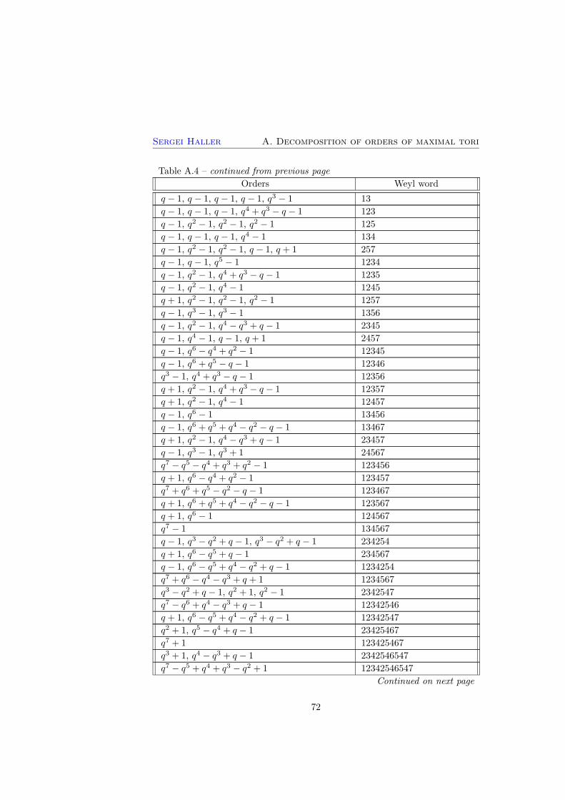
Sergei Haller A. Decomposition of orders of maximal tori
Table A.4 – continued from previous page
Orders Weyl word
q − 1, q − 1, q − 1, q − 1, q3 − 1 13
q − 1, q − 1, q − 1, q4 + q3 − q − 1 123
q − 1, q2 − 1, q2 − 1, q2 − 1 125
q − 1, q − 1, q − 1, q4 − 1 134
q − 1, q2 − 1, q2 − 1, q − 1, q + 1 257
q − 1, q − 1, q5 − 1 1234
q − 1, q2 − 1, q4 + q3 − q − 1 1235
q − 1, q2 − 1, q4 − 1 1245
q + 1, q2 − 1, q2 − 1, q2 − 1 1257
q − 1, q3 − 1, q3 − 1 1356
q − 1, q2 − 1, q4 − q3 + q − 1 2345
q − 1, q4 − 1, q − 1, q + 1 2457
q − 1, q6 − q4 + q2 − 1 12345
q − 1, q6 + q5 − q − 1 12346
q3 − 1, q4 + q3 − q − 1 12356
q + 1, q2 − 1, q4 + q3 − q − 1 12357
q + 1, q2 − 1, q4 − 1 12457
q − 1, q6 − 1 13456
q − 1, q6 + q5 + q4 − q2 − q − 1 13467
q + 1, q2 − 1, q4 − q3 + q − 1 23457
q − 1, q3 − 1, q3 + 1 24567
q7 − q5 − q4 + q3 + q2 − 1 123456
q + 1, q6 − q4 + q2 − 1 123457
q7 + q6 + q5 − q2 − q − 1 123467
q + 1, q6 + q5 + q4 − q2 − q − 1 123567
q + 1, q6 − 1 124567
q7 − 1 134567
q − 1, q3 − q2 + q − 1, q3 − q2 + q − 1 234254
q + 1, q6 − q5 + q − 1 234567
q − 1, q6 − q5 + q4 − q2 + q − 1 1234254
q7 + q6 − q4 − q3 + q + 1 1234567
q3 − q2 + q − 1, q2 + 1, q2 − 1 2342547
q7 − q6 + q4 − q3 + q − 1 12342546
q + 1, q6 − q5 + q4 − q2 + q − 1 12342547
q2 + 1, q5 − q4 + q − 1 23425467
q7 + 1 123425467
q3 + 1, q4 − q3 + q − 1 2342546547
q7 − q5 + q4 + q3 − q2 + 1 12342546547
Continued on next page
72
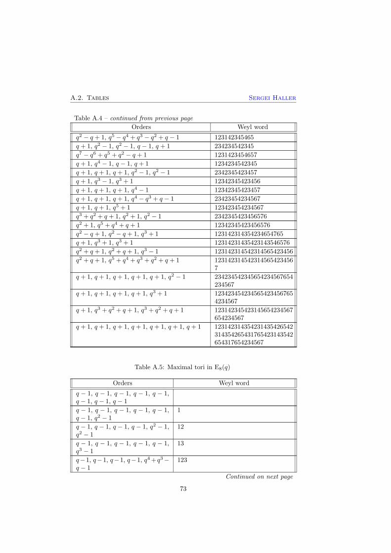
A.2. Tables Sergei Haller
Table A.4 – continued from previous page
Orders Weyl word
q2 − q + 1, q5 − q4 + q3 − q2 + q − 1 123142345465
q + 1, q2 − 1, q2 − 1, q − 1, q + 1 234234542345
q7 − q6 + q5 + q2 − q + 1 1231423454657
q + 1, q4 − 1, q − 1, q + 1 1234234542345
q + 1, q + 1, q + 1, q2 − 1, q2 − 1 2342345423457
q + 1, q3 − 1, q3 + 1 12342345423456
q + 1, q + 1, q + 1, q4 − 1 12342345423457
q + 1, q + 1, q + 1, q4 − q3 + q − 1 23423454234567
q + 1, q + 1, q5 + 1 123423454234567
q3 + q2 + q + 1, q2 + 1, q2 − 1 2342345423456576
q2 + 1, q5 + q4 + q + 1 12342345423456576
q2 − q + 1, q2 − q + 1, q3 + 1 123142314354234654765
q + 1, q3 + 1, q3 + 1 12314231435423143546576
q2 + q + 1, q2 + q + 1, q3 − 1 123142314542314565423456
q2 + q + 1, q5 + q4 + q3 + q2 + q + 1 1231423145423145654234567
q + 1, q + 1, q + 1, q + 1, q + 1, q2 − 1 234234542345654234567654234567
q + 1, q + 1, q + 1, q + 1, q3 + 1 1234234542345654234567654234567
q + 1, q3 + q2 + q + 1, q3 + q2 + q + 1 123142345423145654234567654234567
q + 1, q + 1, q + 1, q + 1, q + 1, q + 1, q + 1 123142314354231435426542314354265431765423143542654317654234567
Table A.5: Maximal tori in E8(q)
Orders Weyl word
q − 1, q − 1, q − 1, q − 1, q − 1,q − 1, q − 1, q − 1
q − 1, q − 1, q − 1, q − 1, q − 1,q − 1, q2 − 1
1
q − 1, q − 1, q − 1, q − 1, q2 − 1,q2 − 1
12
q − 1, q − 1, q − 1, q − 1, q − 1,q3 − 1
13
q−1, q−1, q−1, q−1, q4+q3−q − 1
123
Continued on next page
73
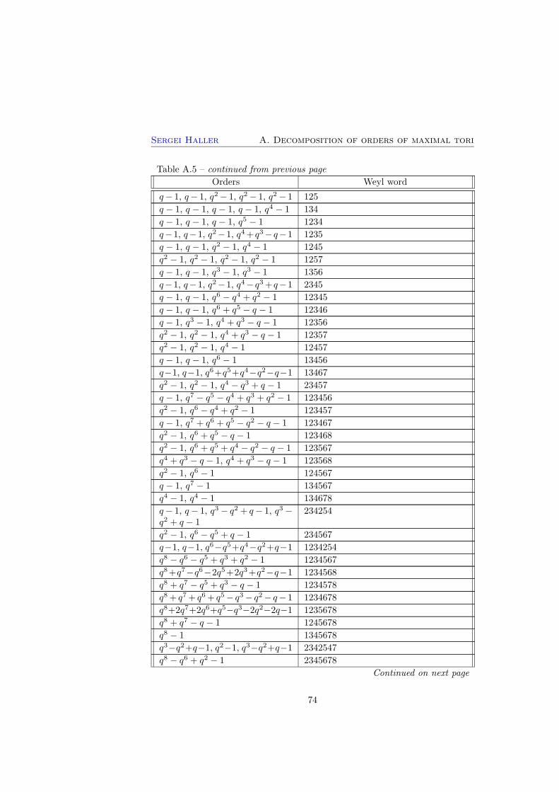
Sergei Haller A. Decomposition of orders of maximal tori
Table A.5 – continued from previous page
Orders Weyl word
q− 1, q− 1, q2− 1, q2− 1, q2− 1 125
q − 1, q − 1, q − 1, q − 1, q4 − 1 134
q − 1, q − 1, q − 1, q5 − 1 1234
q−1, q−1, q2−1, q4+q3−q−1 1235
q − 1, q − 1, q2 − 1, q4 − 1 1245
q2 − 1, q2 − 1, q2 − 1, q2 − 1 1257
q − 1, q − 1, q3 − 1, q3 − 1 1356
q−1, q−1, q2−1, q4−q3+q−1 2345
q − 1, q − 1, q6 − q4 + q2 − 1 12345
q − 1, q − 1, q6 + q5 − q − 1 12346
q − 1, q3 − 1, q4 + q3 − q − 1 12356
q2 − 1, q2 − 1, q4 + q3 − q − 1 12357
q2 − 1, q2 − 1, q4 − 1 12457
q − 1, q − 1, q6 − 1 13456
q−1, q−1, q6+q5+q4−q2−q−1 13467
q2 − 1, q2 − 1, q4 − q3 + q − 1 23457
q − 1, q7 − q5 − q4 + q3 + q2 − 1 123456
q2 − 1, q6 − q4 + q2 − 1 123457
q − 1, q7 + q6 + q5 − q2 − q − 1 123467
q2 − 1, q6 + q5 − q − 1 123468
q2 − 1, q6 + q5 + q4 − q2 − q − 1 123567
q4 + q3 − q − 1, q4 + q3 − q − 1 123568
q2 − 1, q6 − 1 124567
q − 1, q7 − 1 134567
q4 − 1, q4 − 1 134678
q− 1, q− 1, q3 − q2 + q− 1, q3 −q2 + q − 1
234254
q2 − 1, q6 − q5 + q − 1 234567
q−1, q−1, q6−q5+q4−q2+q−1 1234254
q8 − q6 − q5 + q3 + q2 − 1 1234567
q8+q7−q6−2q5+2q3+q2−q−1 1234568
q8 + q7 − q5 + q3 − q − 1 1234578
q8+ q7+ q6+ q5− q3− q2− q− 1 1234678
q8+2q7+2q6+q5−q3−2q2−2q−1 1235678
q8 + q7 − q − 1 1245678
q8 − 1 1345678
q3−q2+q−1, q2−1, q3−q2+q−1 2342547
q8 − q6 + q2 − 1 2345678
Continued on next page
74

A.2. Tables Sergei Haller
Table A.5 – continued from previous page
Orders Weyl word
q − 1, q7 − q6 + q4 − q3 + q − 1 12342546
q2 − 1, q6 − q5 + q4 − q2 + q − 1 12342547
q8 + q7 − q5 − q4 − q3 + q + 1 12345678
q3 − q2 + q − 1, q5 − q4 + q − 1 23425467
q8 − q7 + q − 1 123425467
q8 − q6 + q5 − q3 + q2 − 1 123425468
q8 + q6 − q2 − 1 123425478
q8− q7+ q6− q5+ q3− q2+ q− 1 234254678
q2 − 1, q6 − 1 1234254278
q8 − q4 + 1 1234254678
q4 − q3 + q − 1, q4 − q3 + q − 1 2342546547
q8−q7−q6+2q5−2q3+q2+q−1 12342546547
q8 − q7 + q5 − q3 + q − 1 23425465478
q3 − 2q2 + 2q − 1, q5 − q4 + q3 −q2 + q − 1
123142345465
q3 − q2 + q − 1, q5 + q3 − q2 − 1 123142345478
q8 − q6 + q4 − q2 + 1 123425465478
q2 − 1, q2 − 1, q− 1, q+1, q− 1,q + 1
234234542345
q8−2q7+2q6−q5+q3−2q2+2q−1 1231423454657
q2−q+1, q2−q+1, q4+q3−q−1 1231423454658
q4 − 1, q − 1, q + 1, q − 1, q + 1 1234234542345
q+1, q+1, q2− 1, q2− 1, q2− 1 2342345423457
q2 − q + 1, q6 − q3 + 1 12314234546578
q − 1, q + 1, q3 − 1, q3 + 1 12342345423456
q + 1, q + 1, q2 − 1, q4 − 1 12342345423457
q+1, q+1, q2−1, q4−q3+q−1 23423454234567
q + 1, q + 1, q6 − q5 + q − 1 123423454234567
q + 1, q + 1, q6 − 1 123423454234568
q+1, q+1, q6+q5+q4−q2−q−1 123423454234578
q + 1, q + 1, q6 − q4 + q2 − 1 234234542345678
q8 − q7 + q5 − q4 + q3 − q + 1 1231423454657658
q + 1, q7 + q6 − q4 − q3 + q + 1 1234234542345678
q2 + 1, q2 − 1, q2 + 1, q2 − 1 2342345423456576
q2 + 1, q4 + 1, q2 − 1 12342345423456576
q+1, q+1, q6−q5+q4−q2+q−1 23423454234565768
q + 1, q7 + 1 123423454234565768
q4 − q2 + 1, q4 − q2 + 1 12314234542365476548
Continued on next page
75
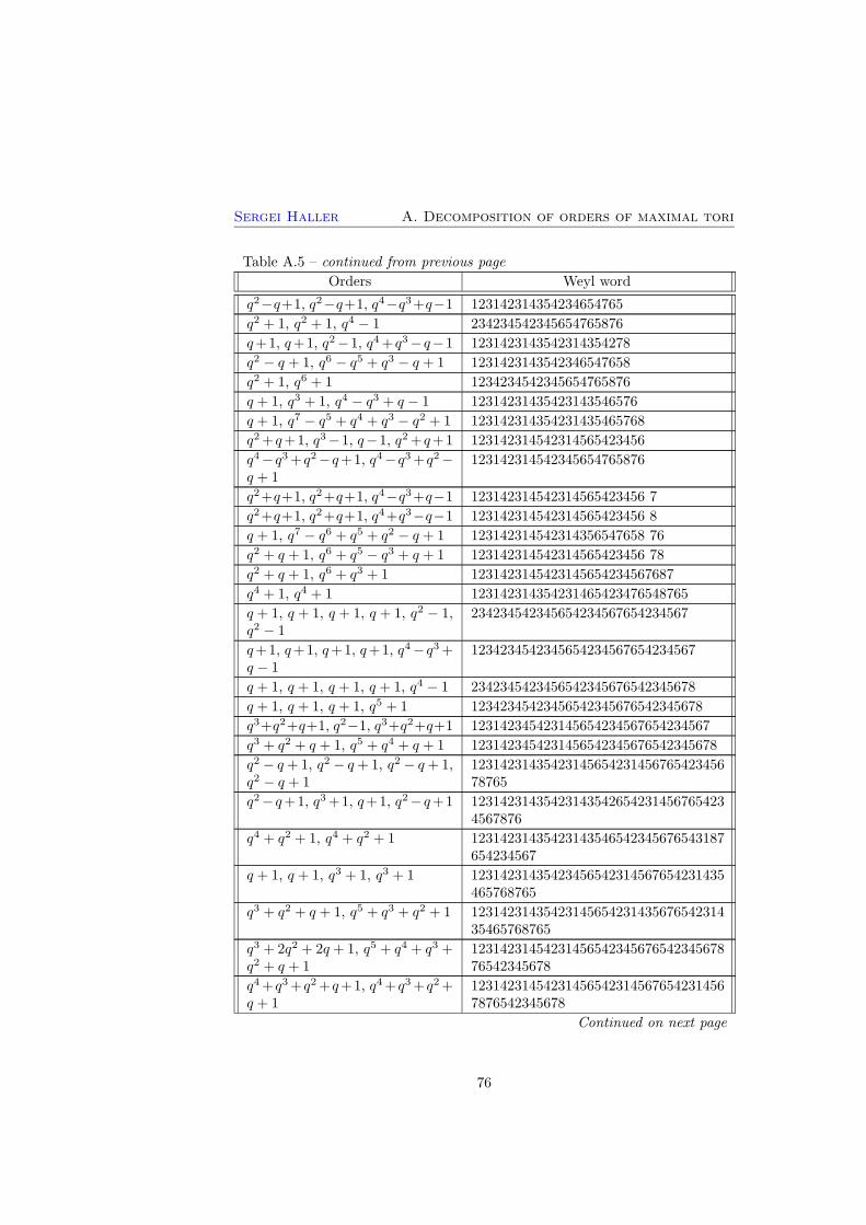
Sergei Haller A. Decomposition of orders of maximal tori
Table A.5 – continued from previous page
Orders Weyl word
q2−q+1, q2−q+1, q4−q3+q−1 123142314354234654765
q2 + 1, q2 + 1, q4 − 1 234234542345654765876
q+1, q+1, q2−1, q4+q3−q−1 1231423143542314354278
q2 − q + 1, q6 − q5 + q3 − q + 1 1231423143542346547658
q2 + 1, q6 + 1 1234234542345654765876
q + 1, q3 + 1, q4 − q3 + q − 1 12314231435423143546576
q + 1, q7 − q5 + q4 + q3 − q2 + 1 123142314354231435465768
q2+q+1, q3−1, q−1, q2+q+1 123142314542314565423456
q4−q3+q2−q+1, q4−q3+q2−q + 1
123142314542345654765876
q2+q+1, q2+q+1, q4−q3+q−1 123142314542314565423456 7
q2+q+1, q2+q+1, q4+q3−q−1 123142314542314565423456 8
q + 1, q7 − q6 + q5 + q2 − q + 1 123142314542314356547658 76
q2 + q + 1, q6 + q5 − q3 + q + 1 123142314542314565423456 78
q2 + q + 1, q6 + q3 + 1 1231423145423145654234567687
q4 + 1, q4 + 1 123142314354231465423476548765
q + 1, q + 1, q + 1, q + 1, q2 − 1,q2 − 1
234234542345654234567654234567
q+1, q+1, q+1, q+1, q4−q3+q − 1
1234234542345654234567654234567
q + 1, q + 1, q + 1, q + 1, q4 − 1 2342345423456542345676542345678
q + 1, q + 1, q + 1, q5 + 1 12342345423456542345676542345678
q3+q2+q+1, q2−1, q3+q2+q+1 123142345423145654234567654234567
q3 + q2 + q + 1, q5 + q4 + q + 1 1231423454231456542345676542345678
q2 − q+ 1, q2 − q+ 1, q2 − q+ 1,q2 − q + 1
1231423143542314565423145676542345678765
q2−q+1, q3+1, q+1, q2−q+1 123142314354231435426542314567654234567876
q4 + q2 + 1, q4 + q2 + 1 12314231435423143546542345676543187654234567
q + 1, q + 1, q3 + 1, q3 + 1 12314231435423456542314567654231435465768765
q3 + q2 + q + 1, q5 + q3 + q2 + 1 1231423143542314565423143567654231435465768765
q3 + 2q2 + 2q + 1, q5 + q4 + q3 +q2 + q + 1
1231423145423145654234567654234567876542345678
q4+q3+q2+q+1, q4+q3+q2+q + 1
123142314542314565423145676542314567876542345678
Continued on next page
76

A.2. Tables Sergei Haller
Table A.5 – continued from previous page
Orders Weyl word
q2 + 1, q2 + 1, q2 + 1, q2 + 1 123142314354231435426542345765423143548765423143542654765876
q + 1, q + 1, q + 1, q + 1, q + 1,q + 1, q2 − 1
123142314354231435426542314354265431765423143542654317654234567
q + 1, q + 1, q + 1, q + 1, q + 1,q3 + 1
1231423143542314354265423143542654317654231435426543176542345678
q+1, q+1, q3 + q2 + q+1, q3 +q2 + q + 1
123142314354231435426542314354265431765423143542654317876542345678
q2 + q+ 1, q2 + q+ 1, q2 + q+ 1,q2 + q + 1
12314231435423143565423143542676542314354265431787654231435426543176542345678765
q + 1, q + 1, q + 1, q + 1, q + 1,q + 1, q + 1, q + 1
123142314354231435426542314354265431765423143542654317654234567876542314354265431765423456787654231435426543176542345678
Table A.6: Maximal tori in 2A5(q)
Orders Weyl word
q − 1, q2 − 1, q2 − 1
q − 1, q2 − 1, q2 − 1 24
q + 1, q2 − 1, q2 − 1 23432
q2 − q + 1, q3 + 1 32145
q − 1, q4 − 1 2343215
q5 − q4 + q3 − q2 + q − 1 2321432154
q + 1, q4 − 1 123214354321
q + 1, q2 − 1, q2 − 1 2132143215432
q + 1, q + 1, q + 1, q2 − 1 12132432154321
q + 1, q + 1, q + 1, q + 1, q + 1 121321432154321
Table A.7: Maximal tori in 3D4(q)
Orders Weyl word
q − 1, q3 − 1
q4 − q3 + q − 1 134
q2 − q + 1, q2 − q + 1 2134
q2 + q + 1, q2 + q + 1 21324213
Continued on next page
77
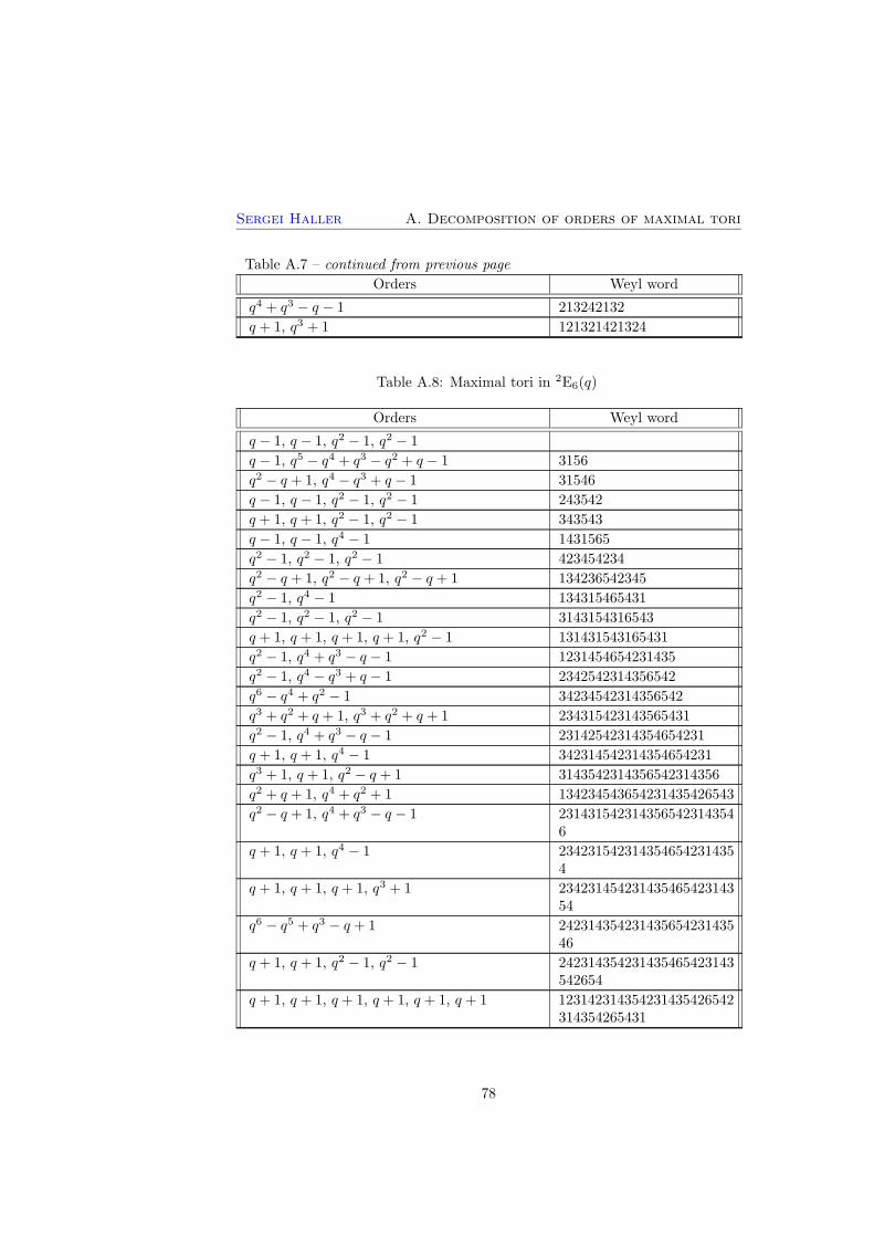
Sergei Haller A. Decomposition of orders of maximal tori
Table A.7 – continued from previous page
Orders Weyl word
q4 + q3 − q − 1 213242132
q + 1, q3 + 1 121321421324
Table A.8: Maximal tori in 2E6(q)
Orders Weyl word
q − 1, q − 1, q2 − 1, q2 − 1
q − 1, q5 − q4 + q3 − q2 + q − 1 3156
q2 − q + 1, q4 − q3 + q − 1 31546
q − 1, q − 1, q2 − 1, q2 − 1 243542
q + 1, q + 1, q2 − 1, q2 − 1 343543
q − 1, q − 1, q4 − 1 1431565
q2 − 1, q2 − 1, q2 − 1 423454234
q2 − q + 1, q2 − q + 1, q2 − q + 1 134236542345
q2 − 1, q4 − 1 134315465431
q2 − 1, q2 − 1, q2 − 1 3143154316543
q + 1, q + 1, q + 1, q + 1, q2 − 1 131431543165431
q2 − 1, q4 + q3 − q − 1 1231454654231435
q2 − 1, q4 − q3 + q − 1 2342542314356542
q6 − q4 + q2 − 1 34234542314356542
q3 + q2 + q + 1, q3 + q2 + q + 1 234315423143565431
q2 − 1, q4 + q3 − q − 1 23142542314354654231
q + 1, q + 1, q4 − 1 342314542314354654231
q3 + 1, q + 1, q2 − q + 1 3143542314356542314356
q2 + q + 1, q4 + q2 + 1 134234543654231435426543
q2 − q + 1, q4 + q3 − q − 1 2314315423143565423143546
q + 1, q + 1, q4 − 1 2342315423143546542314354
q + 1, q + 1, q + 1, q3 + 1 23423145423143546542314354
q6 − q5 + q3 − q + 1 24231435423143565423143546
q + 1, q + 1, q2 − 1, q2 − 1 242314354231435465423143542654
q + 1, q + 1, q + 1, q + 1, q + 1, q + 1 123142314354231435426542314354265431
78

Bibliography
[1] Alejandro Adem and R. James Milgram, Cohomology of finite groups, sec-
ond ed., Grundlehren der Mathematischen Wissenschaften [Fundamental
Principles of Mathematical Sciences], vol. 309, Springer-Verlag, Berlin,
2004. MR 2004k:20109
[2] Shoro Araki, On root systems and an infinitesimal classification of irre-
ducible symmetric spaces, J. Math. Osaka City Univ. 13 (1962), 1–34.
MR 27#3743
[3] Claude Archer, Classification of group extensions, Ph.D. thesis, Universite
Libre de Bruxelles, 2002.
[4] Armand Borel, Linear algebraic groups, Graduate Texts in Mathematics,
vol. 126, Springer-Verlag, New York, 1991. MR 92d:20001
[5] Wieb W. Bosma and J.J. Cannon, The Magma Computational Algebra
System, Tech. report, School of Mathematics and Statistics, University of
Sydney, 1997, http://magma.maths.usyd.edu.au/.
[6] Nicolas Bourbaki, Lie groups and Lie algebras. Chapters 4–6, Elements of
Mathematics (Berlin), Springer-Verlag, Berlin, 2002, Translated from the
1968 French original by Andrew Pressley. MR 1890629 (2003a:17001)
[7] John Cannon and Derek F. Holt, Computing maximal subgroups of finite
groups, J. Symbolic Comput. 37 (2004), no. 5, 589–609. MR 2094616
[8] R. W. Carter, Conjugacy classes in the Weyl group, Compositio Math. 25
(1972), 1–59. MR 47#6884
[9] Roger W. Carter, Simple groups of Lie type, Wiley Classics Library, John
Wiley & Sons Inc., New York, 1989, Reprint of the 1972 original, A Wiley-
Interscience Publication. MR 90g:20001
[10] F. Celler, J. Neubuser, and C. R. B. Wright, Some remarks on the compu-
tation of complements and normalizers in soluble groups, Acta Appl. Math.
21 (1990), no. 1-2, 57–76. MR 1085773 (91m:20026)
79
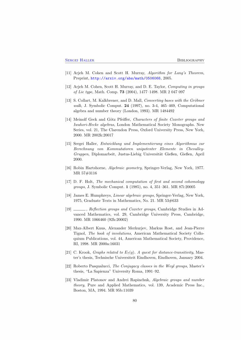
Sergei Haller Bibliography
[11] Arjeh M. Cohen and Scott H. Murray, Algorithm for Lang’s Theorem,
Preprint, http://arxiv.org/abs/math/0506068, 2005.
[12] Arjeh M. Cohen, Scott H. Murray, and D. E. Taylor, Computing in groups
of Lie type, Math. Comp. 73 (2004), 1477–1498. MR 2 047 097
[13] S. Collart, M. Kalkbrener, and D. Mall, Converting bases with the Grobner
walk, J. Symbolic Comput. 24 (1997), no. 3-4, 465–469, Computational
algebra and number theory (London, 1993). MR 1484492
[14] Meinolf Geck and Gotz Pfeiffer, Characters of finite Coxeter groups and
Iwahori-Hecke algebras, London Mathematical Society Monographs. New
Series, vol. 21, The Clarendon Press, Oxford University Press, New York,
2000. MR 2002k:20017
[15] Sergei Haller, Entwicklung und Implementierung eines Algorithmus zur
Berechnung von Kommutatoren unipotenter Elemente in Chevalley-
Gruppen, Diplomarbeit, Justus-Liebig Universitat Gießen, Gießen, April
2000.
[16] Robin Hartshorne, Algebraic geometry, Springer-Verlag, New York, 1977.
MR 57#3116
[17] D. F. Holt, The mechanical computation of first and second cohomology
groups, J. Symbolic Comput. 1 (1985), no. 4, 351–361. MR 87i:20005
[18] James E. Humphreys, Linear algebraic groups, Springer-Verlag, New York,
1975, Graduate Texts in Mathematics, No. 21. MR 53#633
[19] , Reflection groups and Coxeter groups, Cambridge Studies in Ad-
vanced Mathematics, vol. 29, Cambridge University Press, Cambridge,
1990. MR 1066460 (92h:20002)
[20] Max-Albert Knus, Alexander Merkurjev, Markus Rost, and Jean-Pierre
Tignol, The book of involutions, American Mathematical Society Collo-
quium Publications, vol. 44, American Mathematical Society, Providence,
RI, 1998. MR 2000a:16031
[21] C. Krook, Graphs related to E7(q). A quest for distance-transitivity, Mas-
ter’s thesis, Technische Universiteit Eindhoven, Eindhoven, January 2004.
[22] Roberto Pasqualucci, The Conjugacy classes in the Weyl groups, Master’s
thesis, “La Sapienza” University Roma, 1991–92.
[23] Vladimir Platonov and Andrei Rapinchuk, Algebraic groups and number
theory, Pure and Applied Mathematics, vol. 139, Academic Press Inc.,
Boston, MA, 1994. MR 95b:11039
80

Bibliography Sergei Haller
[24] Gopal Prasad, Louis Rowen, and Yoav Segev, Normal subgroups of Quater-
nion algebras and the Whitehead group of algebraic gtoups of type 3,6D4,
Preprint, 2004.
[25] M. S. Raghunathan, Tori in quasi-split-groups, J. Ramanujan Math. Soc.
19 (2004), no. 4, 281–287. MR 2125504
[26] Remko Jurien Riebeek, Computations in association schemes, Thesis Pub-
lishers, Amsterdam, 1998, Dissertation, Technische Universiteit Eindhoven,
Eindhoven, 1998. MR 99d:05089
[27] I. Satake, Classification theory of semi-simple algebraic groups, Marcel
Dekker Inc., New York, 1971, With an appendix by M. Sugiura, Notes
prepared by Doris Schattschneider, Lecture Notes in Pure and Applied
Mathematics, 3. MR 47#5135
[28] Doris J. Schattschneider, On restricted roots of semi-simple algebraic
groups, J. Math. Soc. Japan 21 (1969), 94–115. MR 38 #4485
[29] Martin Selbach, Klassifikationstheorie halbeinfacher algebraischer Gruppen,
Mathematisches Institut der Universitat Bonn, Bonn, 1976, Diplomarbeit,
Univ. Bonn, Bonn, 1973, Bonner Mathematische Schriften, Nr. 83. MR 55
#5759
[30] Jean-Pierre Serre, Galois cohomology, Springer Monographs in Mathemat-
ics, Springer-Verlag, Berlin, 2002. MR 2002i:12004
[31] T. A. Springer and R. Steinberg, Conjugacy classes, Seminar on Alge-
braic Groups and Related Finite Groups (The Institute for Advanced
Study, Princeton, N.J., 1968/69), Lecture Notes in Mathematics, Vol. 131,
Springer, Berlin, 1970, pp. 167–266. MR 42#3091
[32] Tonny A. Springer, Linear algebraic groups, Progress in Mathematics,
vol. 9, Birkhauser Boston Inc., Boston, MA, 1998. MR 99h:20075
[33] Helmut Strade, Simple Lie algebras over fields of positive characteristic. I,
de Gruyter Expositions in Mathematics, vol. 38, Walter de Gruyter & Co.,
Berlin, 2004, Structure theory. MR 2 059 133
[34] Helmut Strade and Rolf Farnsteiner, Modular Lie algebras and their repre-
sentations, Monographs and Textbooks in Pure and Applied Mathematics,
vol. 116, Marcel Dekker Inc., New York, 1988. MR 89h:17021
[35] Franz Georg Timmesfeld, Abstract root subgroups and simple groups of Lie
type, Monographs in Mathematics, vol. 95, Birkhauser Verlag, Basel, 2001.
MR 1852057 (2002f:20070)
81
Sergei Haller Bibliography
[36] J. Tits, Normalisateurs de tores. I. Groupes de Coxeter Etendus, J. Algebra
4 (1966), 96–116. MR 34#5942
[37] Jacques Tits, Classification of algebraic semisimple groups, Algebraic
Groups and Discontinuous Subgroups (Proc. Sympos. Pure Math., Boul-
der, Colo., 1965), Amer. Math. Soc., Providence, R.I., 1966, pp. 33–62.
MR 37#309
[38] , Groupes de Whitehead de groupes algebriques simples sur un corps
(d’apres V. P. Platonov et al.), Seminaire Bourbaki, 29e annee (1976/77),
Lecture Notes in Math., vol. 677, Springer, Berlin, 1978, pp. Exp. No. 505,
pp. 218–236. MR 521771 (80d:12008)
[39] Jacques Tits and Richard M. Weiss, Moufang polygons, Springer Mono-
graphs in Mathematics, Springer-Verlag, Berlin, 2002. MR 2003m:51008
82
Index
Symbols
∗-action . . . . . . . . . . . . . . . . . . . . 7, 28
1-cocycle . . . . . . . . . . . . . . . . . . . . . . 3
2-cocycle . . . . . . . . . . . . . . . . . . . . . . 4
Γ-group . . . . . . . . . . . . . . . . . . . . . . . . 3
Γ-homomorphism . . . . . . . . . . . . . . 5
Γ-set . . . . . . . . . . . . . . . . . . . . . . . . . . 3
Γ-subgroup . . . . . . . . . . . . . . . . . . . . 3
Γ-subset . . . . . . . . . . . . . . . . . . . . . . . 3
Oα(χ) . . . . . . . . . . . . . . . . . . . . . . . . 40
α(a) . . . . . . . . . . . . . . . . . . . . . . . . . . . 4
[[ ]] . . . . . . . . . . . . . . . . . . . . . . . . . . . . . 6
[O]α(r) . . . . . . . . . . . . . . . . . . . . . . . 41
A
absolute rank . . . . . . . . . . . . . . . . . 41
affine space . . . . . . . . . . . . . . . . . . . 19
algebraic automorphism . . . . . . 21
algebraic group
affine . . . . . . . . . . . . . . . . . . . . 20
k-split . . . . . . . . . . . . . . . . . . . 23
linear . . . . . . . . . . . . . . . . . . . . 21
unipotent . . . . . . . . . . . . . . . . 22
algebraic homomorphism . . . . . 21
algebraic isomorphism . . . . . . . . 21
anisotropic kernel . . . . . . . . . . . . . 43
Aut(G) . . . . . . . . . . . . . . . . . . . . . . . 27
AutK(G) . . . . . . . . . . . . . . . . . . . . . 27
C
Cartan subgroup . . . . . . . . . . . . . 22
closed subset . . . . . . . . . . . . . . . . . 20
coboundary . . . . . . . . . . . . . . . . . . . . 4
cocycle
1-cocycle . . . . . . . . . . . . . . . . . . 3
2-cocycle . . . . . . . . . . . . . . . . . . 4
cohomological dimension ≤ 1
of a field . . . . . . . . . . . . . . . . . 30
cohomologous
1-cocycles . . . . . . . . . . . . . . . . . 4
2-cocycles . . . . . . . . . . . . . . . . . 4
connected
component . . . . . . . . . . . . . . . 22
set . . . . . . . . . . . . . . . . . . . . . . . 21
coroots . . . . . . . . . . . . . . . . . . . . . . . 24
D
defined over k
algebraic group . . . . . . . . . . 20
diagram automorphism . . . . . . . 27
dimension of algebraic group . . 20
Dynkin diagram . . . . . . . . . . . . . . 24
E
exact sequence . . . . . . . . . . . . . . . . . 8
extension
of a cocycle . . . . . . . . . . . . . . 11
F
field automorphism . . . . . . . . . . . 27
functorial property . . . . . . . . . . . . . 5
G
Galois cohomology . . . . . . . . . . . . 28
group of Lie type
twisted . . . . . . . . . . . . . . . . . . . 28
untwisted . . . . . . . . . . . . . . . . 26
I
identity component . . . . . . . . . . . 22
83

Sergei Haller Index
inner form . . . . . . . . . . . . . . . . . . . . 41
irreducible . . . . . . . . . . . . . . . . . . . . 21
irreducible components . . . . . . . 21
irreducible root datum . . . . . . . . 24
K
k-anisotropic torus . . . . . . . . . . . . 22
K-rational points . . . . . . . . . . . . . 20
k-split
algebraic group . . . . . . . . . . 23
torus . . . . . . . . . . . . . . . . . . . . . 22
k-torus . . . . . . . . . . . . . . . . . . . . . . . 22
kernel of a map of pointed sets 8
L
Lie type . . . . Ã group of Lie type
linear algebraic group . . . . . . . . . 21
M
maximal torus . . . . . . . . . . . . . . . . 22
morphism of pointed sets . . . . . . 5
morphism of varieties . . . . . . . . . 19
N
nice prime . . . . . . . . . . . . . . . . . . . . 67
O
outer form . . . . . . . . . . . . . . . . . . . . 41
P
pointed set . . . . . . . . . . . . . . . . . . . . 4
morphism of . . . . . . . . . . . . . . 5
polynomial with field auto-
morphisms . . . . . . . . . . 34
R
radical . . . . . . . . . . . . . . . . . . . . . . . . 23
rank
of algebraic group . . . . . . . . 22
reductive . . . . . . . . . . . . . . . . . 23
semisimple . . . . . . . . . . . . . . . 23
rational
torus . . . . . . . . . . . . . . . . . . . . . 63
reduced root datum . . . . . . . . . . . 24
reductive
algebraic group . . . . . . . . . . 23
rank . . . . . . . . . . . . . . . . . . . . . 23
reflections . . . . . . . . . . . . . . . . . . . . 24
relative rank . . . . . . . . . . . . . . . . . . 41
relative root elements . . . . . 45, 46
relative root subgroups . . . . 45, 46
relative root system . . . . . . . . . . . 40
root datum . . . . . . . . . . . . . . . . . . . 24
irreducible . . . . . . . . . . . . . . . 24
reduced . . . . . . . . . . . . . . . . . . 24
root elements . . . . . . . . . . . . . . . . . 26
root subgroup . . . . . . . . . . . . . . . . 27
root system
relative . . . . . . . . . . . . . . . . . . 40
roots . . . . . . . . . . . . . . . . . . . . . . . . . 24
S
semidirect product . . . . . . . . . . . . 17
semisimple
algebraic group . . . . . . . . . . 23
element . . . . . . . . . . . . . . . . . . 22
part . . . . . . . . . . . . . . . . . . . . . . 22
rank . . . . . . . . . . . . . . . . . . . . . 23
Steinberg presentation . . . . . . . . 26
T
Tits index . . . . . . . . . . . . . . . . . . . . 43
torus . . . . . . . . . . . . . . . . . . . . . . . . . 22
k- . . . . . . . . . . . . . . . . . . . . . . . . 22
k-anisotropic . . . . . . . . . . . . . 22
k-split . . . . . . . . . . . . . . . . . . . 22
trivial 1-cocycle . . . . . . . . . . . . . . . . 3
twisted form . . . . . . . . . . . . . . . 7, 28
twisted group of Lie type . . . . . 28
twisting . . . . . . . . . . . . . . . . . . . . . . . . 7
U
unipotent
algebraic group . . . . . . . . . . 22
element . . . . . . . . . . . . . . . . . . 22
part . . . . . . . . . . . . . . . . . . . . . . 22
radical . . . . . . . . . . . . . . . . . . . 23
84

Index Sergei Haller
V
variety
affine algebraic . . . . . . . . . . . 19
W
Weyl group . . . . . . . . . . . . . . . . . . . 24
Z
Zarisski topology . . . . . . . . . . . . . 20
zero set . . . . . . . . . . . . . . . . . . . . . . . 19
85
Samenvatting
Om op een efficiente manier te rekenen met groepen is een geschikte voorstelling
nodig van de groepselementen. Een groep heeft vaak een intrinsieke defini-
tie, dat wil zeggen dat zij impliciet gedefinieerd wordt door een beschrijving
van de eigenschappen van de elementen (bijv.: de vaste punt ondergroep van
een groep). Een dergelijke definitie is voor berekeningen met groepselementen
niet erg handig aangezien het, afgezien van de identiteit, geen construeerbare
groepselementen geeft. In dergelijke gevallen dient men te beschikken over een
extrinsieke definitie van de groep, zoals een voorstelling.
Wij ontwerpen en implementeren algoritmen voor berekeningen aan gedraaide
groepen van Lie-type, waaronder begrepen zijn de groepen die niet quasi-gesple-
ten zijn. Algoritmen voor het rekenen met elementen in de Steinberg voorstelling
voor ongedraaide groepen van Lie-type en algoritmen voor de overgang tussen
deze voorstelling en de lineaire representatie worden gegeven in [12] (gebaseerd
op werk van [15] en [26]). Dit werk wordt in diverse richtingen uitgebreid.
De gedraaide groepen van Lie-type zijn groepen van rationale punten van
gedraaide vormen van reductieve lineaire algebraısche groepen. De gedraaide
vormen zijn geclassificeerd door Galoiscohomologie. Ten einde de Galoisco-
homologie te berekenen ontwerpen we een methode voor het berekenen van de
cohomologie van een eindig voortgebrachte groep Γ op een groep A. Deze meth-
ode is op zichzelf van belang. De methode wordt toegepast op de berekening
van de Galoiscohomologie van een reductieve lineaire algebraısche groep.
LaatG een reductieve lineaire algebraısche groep gedefinieerd over een lichaam
k zijn. Een gedraaide groep van Lie-type Gα(k) wordt uniek bepaald door de co-
cykel α van de Galois groep van K op AutK(G), en de groep van K-algebraısche
automorfismen waar K de eindige Galoisuitbreiding over k is. Algoritmen voor
de berekening van het relatieve wortelsysteem op Gα(k), voor de wortelonder-
groepen en de wortelelementen worden gegeven. Daarnaast worden ook algo-
ritmen voor de berekening van onderlinge relaties, zoals de commutatorrelaties
en producten gegeven. Dit maakt het mogelijk om te rekenen binnen de nor-
male ondergroep Gα(k)† van Gα(k) voortgebracht door de wortelelementen.
We passen het algoritme toe op diverse voorbeelden, waaronder 2E6,1(k) en3,6D4,1(k).
87
Sergei Haller Samenvatting
Een toepassing is een algoritme, ontworpen voor de berekening van alle gedraai-
de maximale tori van een eindige groep van Lie-type. De orde van zo’n torus
wordt berekend als een polynoom in q, de orde van het lichaam k. Daarnaast
berekenen we de ordes van de faktoren in de decompositie van de torus als een
direkt product van cyklische ondergroepen.
Voor een gegeven lichaam k, worden de maximale tori van Gβ(k) berekend
als ondergroepen van Gβ(K) over een uitbreidingslichaam K en daarna wordt
de effectieve versie van Lang’s Theorem [11] gebruikt om de torus te conjugeren
tot een k-torus, wat een ondergroep van Gβ(k) is.
Gebruikmakend van deze informatie over maximale tori, geven we een algo-
ritme voor de berekening van alle Sylowondergroepen van de groep van Lie-type.
Als p niet de karakteristiek van het lichaam is, wordt de Sylowondergroep berek-
end als een ondergroep van de normalisator van de k-torus.
Alle hier besproken algoritmen zijn geımplementeerd in Magma [5].
88
Acknowledgments
There are many people I would like to thank for helping me (explicitly or im-
plicitly) in this project. First and formost, I would like to express my thanks
to both my supervisors, A.M. Cohen and F.G. Timmesfeld. Prof. Timmesfeld
supervised me starting with my first year as an undergraduate student, during
my diploma thesis and my Ph.D. project. I learned from him the affinity to
abstract algebra and group theory. Prof. Cohen introduced me in the beautiful
world of algebraic groups and guided me through my time as a Ph.D. student.
Without their support and advices, this work would not be possible.
I would like to thank Scott Murray, whose role during my Ph.D. project comes
close to the role of a copromotor. Especially my visit at the University of Sydney
in 2004, where he was employed at that time, was a very important step in my
research.
I would like to thank everybody who expressed interest in my work and in-
spired me to new ideas, without mentioning each name explicitly.
I would like to thank the Departments of Mathematics of the Justus-Liebig
University of Gießen and the Technical University of Eindhoven, where I spent
the last years of my research.
I thank all my friends for just being my friends, especially Nguy˜en Van Minh
M˜an, who was my office and apartment mate during my stays at the Eindhoven
University in the last years.
I would like to thank my parents Nina and Andreas for their support through
all my life.
I would like to thank my wife Natalia for her love.
89
Curriculum Vitae
Sergei Haller was born on March 4th, 1975 in Krasnoturinsk, Russia. He studied
at School Number 9 in Krasnoturinsk from 1982 until 1990, with highest avail-
able marks in all subjects. He studied at Herderschule High School in Gießen,
Germany, in 1990–1994.
After a year in the Bundeswehr, the German army, he started studying
mathematics at the Justus-Liebig Universitat Gießen in 1995. He obtained
his diploma with a thesis entitled Entwicklung und Implementierung eines Algo-
rithmus zur Berechnung von Kommutatoren unipotenter Elemente in Chevalley-
Gruppen [15] (Development and implementation of an algorithm for computing
commutators of unipotent elements in Chevalley groups), which obtained a mark
of 1.0, in April 2000.
He has worked as a scientific assistant at the Mathematics Department of the
Universitat Gießen since May 2000. The present Ph.D. project was started in
September 2002 and supervised by Prof. Arjeh M. Cohen from the Technische
Universitait Eindhoven and Prof. Franz G. Timmesfeld from the Universitat
Gießen.
91


![Galois Cohomology and Algebraic K-theory of Finite Fields · in Weibel’s book on algebraic K-theory, yet to arrive in print [16], and Thomason’s paper on algebraic K-theory and](https://img.dokumen.tips/doc/110x75/5ede2ec1ad6a402d66697cba/galois-cohomology-and-algebraic-k-theory-of-finite-fields-in-weibelas-book-on.jpg)
![Galois and θ Cohomology Jeffrey Adams Vogan …math.mit.edu/conferences/Vogan/images/adams_slides.pdf(see [12, Lemma 2.9]). For more information on Galois cohomology of classical](https://img.dokumen.tips/doc/110x75/5f0ef71f7e708231d441d09a/galois-and-cohomology-jeirey-adams-vogan-mathmiteduconferencesvoganimagesadams.jpg)