Computing Eigenvalues of Singular Sturm-Liouville Problems

P. B. Bailey W. N. Everitt and A. Zettl

November 2, 1999

Abstract

We describe a new algorithm to compute the eigenvalues of singular Sturm-Liouville problemswith separated self-adjoint boundary conditions for both the limit-circle nonoscillatory andoscillatory cases. Also described is a numerical code implementing this algorithm and how itcompares with SLEIGN. The latter is the only effective general purpose software available forthe computation of the eigenvalues of singular Sturm-Liouville problems.

1 Introduction

The code SLEIGN (Sturm-Liouville eigenvalue) was introduced in 1978; see Bailey [3] and [4], andespecially Bailey, Gordon and Shampine [7]. It is a general purpose software package designed tocompute the eigenvalues of (i) SL problems with regular, separated, self-adjoint boundary conditionsand (ii) singular SL problems. In the singular case the code automatically selects a boundarycondition. Thus in the singular limit-circle case the user does not have the option of specifyingwhich of the infinitely many self-adjoint singular boundary conditions are to be used.

The purpose of this article is to describe a basic approximation theorem and a new code calledSLEIGN2. Although it was inspired by SLEIGN it includes a new algorithm which will be describedhere. SLEIGN2 is designed to compute the eigenvalues of any SL problem with separated, self-adjoint boundary conditions. These problems may be regular or singular at each endpoint of theunderlying interval. The user has complete freedom in specifying the boundary conditions as longas these are formulated appropriately in a manner to be described below.

A Sturm-Liouville (SL) boundary value problem consists of a second order linear ordinarydifferential equation

−(py′)′ + qy = λwy on (a, b) (1.1)

and boundary conditions. Here I = (a, b) is a bounded or unbounded open interval of the realline R i.e. −∞ ≤ a < b ≤ ∞; the coefficients p, q, w : (a, b) into R; λ ∈ C, the complex field. Inorder that (1.1) have solutions in an appropriate sense certain additional restrictions are placedon p, q and w to be specified in Section 2. The nature of the boundary conditions depends on theclassification of the endpoints as regular or singular. These will also be given in Section 2.

In general non-trivial solutions of (1.1) satisfying the imposed boundary conditions only exist forcertain distinguished values of the parameter λ; these are the so-called eigenvalues of the problem.

1

The determination of the eigenvalues of SL problems is of great interest in mathematics and itsapplications. Their numerical calculation is of considerable importance in numerical analysis andis a meeting ground for analysis, numerical analysis and applied mathematics.

SLEIGN is remarkably successful. For regular problems the only comparable code is DO2KEFin the NAG Library [9]. Both are very effective in the regular case. But in the singular case SLEIGNhas no serious competitor. Both codes are based on the Prufer transformation and on a knowledgeof the precise number of zeros of the eigenfunctions. The linear second order differential equation(1.1) is transformed into a nonlinear first order differential equation for the phase function whichcan be integrated efficiently and dependably. The computation of a specified eigenvalue requiresknowledge of the precise number of zeros of its eigenfunction but does not require any knowledgeof either preceding or subsequent eigenvalues. Thus, in principle, each eigenvalue is computedindependently and to any described accuracy. SLEIGN will make use of an initial guess if one isprovided, but otherwise has its own guesstimator written into the program.

The equation for the phase function has the form

θ′ = p−1cos2θ + (λw − q)sin2θ on (a, b). (1.2)

If a is a finite singular endpoint and p(a) = 0, it is clear from (1.2) that θ′(a) becomes infinitefor all initial conditions θ(a) = α, 0 ≤ α < π, with the possible exception of α = π/2. Similarly,at a singular endpoint at which w or q is unbounded θ′ becomes infinite for all initial conditions0 ≤ α < π with one possible exception. SLEIGN takes advantage of these exceptional cases whensearching for a possible boundary condition. It is clear that for all the nonexceptional cases theobstacles are formidable. This is why a new code SLEIGN2 is being developed.

As previously mentioned SLEIGN is the only available general purpose code which is effectivefor a wide range of singular SL problems. These occur when at least one of the coefficients p−1, q, wis not integrable up to the endpoint (i.e. is unbounded in a suitably severe way) or if one orboth of these endpoints is infinite. Such boundary value problems are termed singular. Thesepresent particular difficulties both in the determination of well-posed problems and in the numericalcalculation of eigenvalues.

We present a brief account of these technical matters in the next section when we recall the well-established limit-point/limit-circle classification of the endpoints of the interval (a, b); see Titch-marsh [25], Chapter II and Naimark [20], p. 73. It suffices here to say that SLEIGN is effective withmany limit-point singularities, when boundary conditions are not required, and with limit-circlesingularities. In the latter case the user does not have an option to specify the boundary condition,since SLEIGN automatically selects a ”special” one within the code. In many cases of interestin mathematical physics this special boundary condition determines the Friedrichs extension. Seethe examples in Bailey [[3], p. 27] and Marletta [19]. For a discussion of the Friedrichs extensionsee Niessen and Zettl [21]. The problem represented by the Friedrichs extension is often of specialimportance in applications.

SLEIGN2 is a general purpose code for limit-circle boundary conditions to be specified by theuser. Both nonoscillatory and oscillatory endpoints are included. The numerical problems in theoscillatory case are particularly difficult. In this case every eigenfunction has an infinite number ofzeros in any neighborhood of the end point. Recall that the algorithm on which SLEIGN is based

2

depends on knowing that, when the eigenvalues are enumerated appropriately, the nth eigenfunctionhas precisely n zeros in the interval (a, b).

It should not be thought that the design of SLEIGN2 to cope with both the non-oscillatoryand the oscillatory limit-circle cases is introduced out of a wish for completeness alone. Both casespresent Strum-Liouville boundary value problems which are of importance in applied mathematicsand mathematical physics. There are many applications for limit-circle non-oscillatory equationsand we have quoted some of these in references [2], [8], [11], [12] and [14]. However, the limit-circleoscillatory equations also play a role in mathematical physics; see [17] and its references.

SLEIGN2 does require the user to distinguish between regular and singular endpoints; in thesingular case the user must further distinguish between the limit-point and limit-circle cases, andin the latter case to describe the boundary condition appropriately as explained below.

All this is an essential feature of SLEIGN2. These classifications of the endpoints and boundaryconditions are not part of the program. They depend on an analytic assessment of the problem.A number of questions for further investigation come to mind. Can SLEIGN be enhanced tohandle continuous spectra in the limit point case? While SLEIGN also computes eigenfunctions,SLEIGN2 computes only eigenvalues. How can eigenfunctions be computed? Can the conditionsp > 0, w > 0 a.e. be relaxed? In particular one wants to study the cases when p or w changesign; see in particular [5], [6] and [14]. We plan to pursue these and other questions in subsequentpapers.

The contents of the paper are as follows. The introduction in Section 1 is followed by a discussionof SL expressions in Section 2. Boundary conditions are discussed in Section 3. The basic approx-imation theorem is stated in Section 4; Section 5 is devoted to a brief description of SLEIGN2.Finally a wide range of examples is discussed in detail in Section 6. The given SLEIGN 2 numericalresults for these examples are intended to illustrate the capability of SLEIGN 2 to handle a varietyof limit-circle problems, including both the nonoscillatory and oscillatory cases, and to allow theuser to select boundary conditions.

Acknowledgements. All three authors are pleased to acknowledge their indebtedness to:1. The Science and Engineering Research Council of the United Kingdom for funding Senior

Visiting Fellowships to enable P.B. Barley and Anton Zettl to visit the University of Birmingham,England in the autumn of 1988 when the programmer on SLEIGN 2 was . We are grateful to Mr.Fred Hemmings, then Secretary to the Mathematics Committee of SERC, for constant help andadvice.

2. The University of Birmingham, England for facilities provided through the Department ofMathematics in the autumn of 1988.

3. Northern Illinois University for financial support and facilities provided through the Depart-ment of Mathematical Sciences during the calendar year 1990.

2 Sturm-Liouville Differential Expressions

Let I denote any interval of the real line R with endpoints a and b where −∞ ≤ a < b ≤ ∞. Acompact, i.e. a bounded and closed interval, is denoted by [a, b] = {t ∈ R : a ≤ t ≤ b} where−∞ < a < b <∞.

3

By L(I) or L1(I) we denote the space of complex valued measurable functions on I for which∫I|y(t)|dt =

∫I|y| <∞. (2.1)

The notation Lloc(I) is used to denote the space of functions y satisfying y ∈ L[α, β] for all compactsubintervals [α, β] of I.

Likewise L2(I) denotes the space (of equivalence classes) of functions y such that∫I|y(t)|2dt <∞;

and if w is a positive measurable function on I then L2(I;w) represents the weighted space offunctions y satisfying ∫

I|y(t)|2w(t)dt <∞. (2.2)

This is a Hilbert space if vectors in the space are determined by equivalence classes of functionsand the inner product is given by

(y, z) =∫Iw(t)y(t)z(t)dt. (2.3)

The bar over z denotes the complex conjugate.Throughout this paper we assume that the coefficients p, q, w satisfy:

p, q, w : I → R (2.4)

p−1, q, w ∈ Lloc(I) (2.5)

p(t) > 0, w(t) > 0, almost everywhere on I. (2.6)

When additional conditions are needed they will be specified.The standard existence theorems for solutions of the differential equation

−(py′)′ + qy = λwy on I, (2.7)

under the conditions (2.4), (2.5), (2.6), can be found in Naimark [20]. By a solution of (2.7) wemean a function y such that y and py′ are both absolutely continuous on all compact subintervalsof I (so that the left hand side of (2.7) is defined a.e. on I) and (2.7) holds a.e. Note that thequasi-derivative py′ is required to be absolutely continuous, the classical derivative y′ may not be.

Definition 2.1 The endpoint a of I is said to be regular if a is finite and

p−1, q, w ∈ L[a, α] for some α in(a, b). (2.8)

Similarly the endpoint b is regular if it is finite and

p−1, q, w ∈ L[β, b] for some β in(a, b). (2.9)

An endpoint is called singular if it is not regular. Thus an endpoint is singular if it is infinite,or the endpoint is finite but at least one of p−1, q, w is not integrable in any neighborhood of theendpoint.

4

The singular endpoint a is classified as limit-circle (LC for short) if all solutions of equation (2.7)are in L2((a, α);w) for some α in I; similarly b is LC if all solutions of (2.7) are in L2((β, b); w) forsome β in I. An endpoint which is not LC is called limit-point or LP for short. It is well known[20, 25] that this LC/LP classification is independent of λ in C, see Weidmann [26, Sections B, 14].

In Section 4 we will need a further subclassification of the LC endpoints into oscillatory andnonoscillatory cases. It follows from condition (2.5) and (2.6) that a nontrivial solution of (1.1)with λ real can only have isolated zeros in (a, b). Thus the zeros of nontrivial solutions of (1.1) canaccumulate only at an endpoint. The endpoint a is called oscillatory (O) if (1.1) has a nontrivialsolution which has a zero in every interval (a, α), a < α < b. Otherwise the endpoint a is callednonoscillatory (NO). Similar definitions are made for b. In the LP case this classification depends onλ. However, given the LC case the O or NO classification is independent of λ in R, see Weidmann[26, Section B, 14].

3 Boundary Conditions

In this section and in fact for the rest of this paper we assume for the differential equation

−(py′)′ + qy = λwy on I = (a, b),−∞ ≤ a < b ≤ ∞,

that each endpoint a, b is either regular or LC. If one or both endpoints are LP either SLEIGN orSLEIGN2 may be used.

Define the quasi-differential expression M by

My = −(py′)′ + qy on I

Define the ”maximal domain” ∆ by ∆ = {y : I → C : y, py′ are absolutely continuous on allcompact subintervals of I, and y, w−1My ∈ L2(I;w)}.

For all functions y, z in ∆ we have the well known Green’s formula∫ β

α{zMy − yMz} = [y, z]βα, α, β ∈ I, (3.1)

where[y, z](t) = (y(pz′)− z(py′))(t) all t ∈ I. (3.2)

It is clear from (3.1) that both limits

[y, z](a) = limt→a+

[y, z](t) and [y, z](b) = limt→b−

[y, z](t), (3.3)

exist and are finite for all y, z in ∆.Choose real valued functions u, v in ∆ with the following properties

[u, v](a) 6= 0 6= [u, v](b). (3.4)

Such a choice is always possible. For example u and v can be any two real linearly independentsolutions of (1.1) for any real value of λ.

5

As shown in Naimark [20] all separated self-adjoint boundary conditions for (1.1) can be for-mulated as follows (for y in ∆):

A1[y, u](a) +A2[y, v](a) = 0 (3.5)

B1[y, u](b) +B2[y, v](b) = 0 (3.6)

where A1, A2, B1, B2 are all real and A21 +A2

2 > 0, B21 +B2

2 > 0.If a is regular and we choose u, v to be real solutions of (1.1) for any particular λ in R, e.g.

λ = 0 satisfyingu(a) = 0, (pu′)(a) = 1, v(a) = 1, (pv′)(a) = 0,

then (3.5) reduces to the more familiar form:

A1y(a) +A2(py′)(a) = 0. (3.7)

Similarly, if b is regular we can choose u and v so that (3.6) reduces to

B1y(b) +B2(py′)(b) = 0. (3.8)

Also it can be shown that if both a and b are regular we can choose u and v so that both (3.5) and(3.6) reduce to (3.8) and (3.9). Thus (3.5) and (3.6) can be viewed as the analogues of (3.8) and(3.9) in the singular LC case.

Another equivalent form of (3.7) and (3.8) is given by

y(a)cos α+ (py′)(a)sin α = 0, 0 ≤ α < π, (3.9)

y(b)cos β + (py′)(b)sin β = 0, 0 < β ≤ π. (3.10)

Remark 3.1 If a is a regular endpoint of the open interval I = (a, b) then for any solution y of(1.1) with λ in C, y(a) and (py′)(a) can be defined by

y(a) = limt→a

y(t), (py′)(a) = limt→a

(py′)(t). (3.11)

These limits exist and are finite.

4 The basic approximation theorem

Throughout this section we assume that each endpoint a or b of the interval I is either regular orlimit-circle.

The differential equation

−(py′)′ + qy = λwy on I = (a, b), −∞ ≤ a < b ≤ ∞, (4.1)

together with the boundary conditions

A1[y, u](a) +A2[y, v](a) = 0, A1, A2 ∈ R, A21 +A2

2 > 0, (4.2)

6

B1[y, u](b) +B2[y, v](b) = 0, B1, B2 ∈ R,B21 +B2

2 > 0, (4.3)

where u and v are real valued functions in ∆ satisfying (3.4), is called a separated Sturm-Liouville(SL) boundary value problem (BVP). (The boundary conditions (4.2), (4.3) are separated; there arealso coupled, i.e. nonseparated conditions which could be used but we will consider only boundaryconditions of type (4.2) and (4.3) in this paper.)

A complex number λ is called an eigenvalue of the BVP if there exists a nontrivial solutionof (4.1) which satisfies (4.2) and (4.3). Such a solution is called an eigenfunction belonging to λor associated with λ. It is well known [see Naimark [20]] that under the conditions (2.4), (2.5)and (2.6) and the assumption that each endpoint is either regular or LC there exist an infinitenumber of eigenvalues. These are all real, countable, isolated and each eigenfunction is unique upto constant multiples.

If each endpoint is in the NO case (this automatically holds at a regular endpoint while it mayor may not hold at an LC endpoint) then, in addition, the eigenvalues are bounded below. Thusthey can be indexed such that

−∞ < λ0 < λ2 < ... and λn →∞ as n→∞. (4.4)

Furthermore, if φn denotes an eigenfunction corresponding to λn, n ∈ N0 = {0, 1, 2, ...}, then φnhas exactly n zeros in the open interval (a, b), see Atkinson [1] and Weidmann [26]. This fact is ofcritical importance in the numerical calculation of the eigenvalues by SLEIGN.

If one or both endpoints is oscillatory, then the eigenvalues are not bounded below. With λn,n ∈ Z = {−2,−1, 0, 1, 2, ...} denoting the eigenvalues and φn the corresponding eigenfunctions wehave, in this case,

... < λ−2 < λ−1 < λ0 < λ1 < λ2..., (4.5)

λn → −∞ as n→ −∞ and λn → +∞ as n→∞, (4.6)

and each eigenfunction φn, n ∈ Z, has infinitely many zeros in (a, b), see again [26]. Note that inthis case when Z is the index set the indexing scheme for λn is rather arbitrary: λ1 in one set mightbe λ83 in another set. To get a definite procedure one can denote the first nonnegative eigenvalueby λ0. The others are then determined by (4.5).

How can the eigenvalues λn be computed numerically?Let P (a, b) represent the BVP consisting of (4.1), (4.2) and (4.3). Recall that u, v are real

members of ∆ satisfying (3.4), p, q, w satisfy (2.4), (2.5) and (2.6) and each endpoint is assumedto be either regular or LC. For α, β in I with a < α < β < b let P [α, β] represent the regular BVPon [α, β] given by

−(py′)′ + qy = λwy on [α, β] (4.7)

A1[y, u](α) +A2[y, v](α) = A1{y(α)(pu′)(α)− u(α)(py′)(α)}+A2{y(α)(pv′)(α)− v(α)(py′)(α) = A1(α)y(α) +A2(α)(py′)(α) = 0 (4.8)

withA1(α) = A1(pu′)(α) +A2(pv′)(α), A2(α) = −A1u(α)−A2v(α), (4.9)

7

andB1[y, u](β) +B2[y, v](β) = B1(β)y(β) +B2(β)(py′)(β) = 0 (4.10)

withB1(β) = B1(pu′)(β) +B2(pv′)(β), B2(β) = −B1u(β)−B2v(β). (4.11)

A basic point of this paper is to claim that the regular BVP P [α, β] is a good approximationof the BVP P (a, b) even if the latter is singular LC at one or both endpoints, when α is ”close”to a and β is ”close” to b. The approximation of P (a, b) by P [α, β] is the basis of our algorithm.However, in our numerical implementation when one or both endpoints are oscillatory we restrictu and v to be real linearly independent solutions of (1.1) for some real value of λ.

Denote the eigenvalues of P (a, b) and P [α, β] by λn(a, b), λn[α, β].If each endpoint a, b is nonoscillatory then the convergence of {λn[α, β]} to λn(a, b) is straight-

forward. However, if a is oscillatory then this ”convergence” is much more complicated since inthis case we have that for each n in N0

λn[α, β]→ −∞ as α→ a and β → b. (4.12)

Yet in spite of (4.12) the eigenvalues of oscillatory problems can be approximated by eigenvaluesfrom regular problems!

Theorem 4.1 Let (2.4), (2.5), (2.6) hold, let a < αk < βk < b, k = 1, 2, 3, ..., and let αk → aand βk → b with αk decreasing and βk increasing. Assume each of a and b is either regular or LC.Suppose λ = λn(a, b) is an eigenvalue of problem P (a, b). Then each open interval containing λcontains an eigenvalue of the regular problem P [αk, βk] for all sufficiently large integers k.

Proof : This will be given in a subsequent paper. It is a consequence of an abstract result inoperator theory; see Kato [[16], p. 371]. To see that this abstract result applies we construct asequence of self-adjoint operators Ak corresponding to problem P [αk, βk] and a self-adjoint operatorA corresponding to problem P (a, b) all in the Hilbert space L2(I, w) such that the sequence Akconverges to A in the sense of norm resolvent convergence.

Theorem 4.1 has the following consequence: Given an eigenvalue λ of the (singular) problemP (a, b) there exists a sequence of eigenvalues chosen from the regular problems P [αk, βk] whichconverges to λ. Since this sequence is constructed differently in the oscillatory and nonoscillatorycases we treat these cases separately below. In the oscillatory case, as we will see in the statementof the construction below, the index of the approximating eigenvalue from the regular problemP [αk, βk] changes with k.

Construction of an approximating sequence Assume the hypotheses and the notation ofTheorem 4.1 hold.

(a) Suppose both endpoints a, b are nonoscillatory. Choose u, v in ∆ satisfying (3.4). Denotethe eigenvalues of problems P (a, b) and P [αk, βk] by λn(a, b) and λn[αk, βk], respectively, with theindex n so chosen that in all cases we have

−∞ < λ0 < λ1 < λ2 < ..., λn →∞ as n→∞. (4.13)

8

Then for any n ∈ N0 we have

λn[αk, βk]→ λn(a, b) as k →∞. (4.14)

(b) Assume at least one of the endpoints a, b is oscillatory. For any fixed but arbitrary λ inR let u, v be real linearly independent solutions of (1.1). (Note that in this case the eigenvaluesλn(a, b) of the singular problem P (a, b) are indexed with n ∈ Z while those of the regular problemsP [αk, βk] i.e. λn[αk, βk] are indexed with n ∈ N0, k = 1, 2, 3, ... In place of (4.13) we have

... < λ−2(a, b) < λ−1(a, b) < λ0(a, b) < λ1(a, b) < λ2(a, b) < ...

withλn(a, b)→ −∞ as n→ −∞; λn(a, b)→∞ as n→∞. (4.15)

Of course we still have

−∞ < λ0[αk, βk] < λ1[αk, βk] < λ2[αk, βk] < ... (4.16)

with λn[αk, βk]→∞ as n→∞ for each k = 1, 2, 3, .... In this case there is no simple approximationcomparable to (4.14). Instead we have the following: Given any λn(a, b), n ∈ Z, there exists asequence of positive integers mk satisfying m1 ≤ m2 ≤ m3 ≤ ... with mk →∞ as k →∞ such that

λmk [αk, βk]→ λn(a, b). (4.17)

The sequence mk depends on the index n in Z.The existence of index sequence mk such that (4.17) holds follows immediately from Theorem

4.1. However the construction of this sequence for a given λn(a, b) is not clear from Theorem 4.1or its proof. We now describe a procedure which can be used to construct an index sequencemk. Find an integer k which is large enough so that among the eigenvalues λr[αk, βk], r ∈ N0 ofproblem P [αk, βk] there is one which is ”close” to λn(a, b). Let m1 be the index of this eigenvalueof the regular problem P [αk, βk]. Count the number of zeros l the ”boundary condition function”A1u+A2v has in the interval (αk+1, αk) and count the number of zeros r the function B1u+B2vhas in the interval (βk, βk+1). Now let m2 = m1 + l+ r, and repeat this process. This procedure isbased on the fact that as αk moves toward αk+1, each time it passes through a zero of the functionA1u+A2v in the interval (αk+1, αk) the problem P [αk+1, βk] “gives birth” to a new eigenvalue tothe left of λ0[αk, βk]. For example if A1u+A2v has three zeros in the interval (αk+1, αk) then theeigenvalues λ0[αk+1, βk] λ1[αk+1, βk], λ2[αk+1, βk] are all considerably to the left of λ0[αk, βk] andλ3[αk+1, βk] is “close” to λ0[αk, βk]. In this case l = 3 in the above scheme. Thus the index “jumps”by 3 due to the three zeros of the boundary condition function A1u+A2v in the interval (αk+1, αk).A similar jump in the index is produced by each zero of the boundary condition function B1u+B2vin the interval (βk, βk+1).

This construction of the index sequence can be simplified if only one end point, say a, isoscillatory. Then for k sufficiently large all the βk are to the right of the right-most zero of thefunction B1u+B2v in the interval (a,b). For such k we have mk+1 = mk+ the number of zeros ofthe function A1u+A2v in the interval (αk+1, αk). Similarly for the case when a is NO and b is O.

9

In the above construction of m1, m2, m3, ... once m1 is selected mk is determined for all k ≥ 2by the above zero counting scheme.

In a subsequent communication, in collaboration with J. Weidmann, it will be shown that if asequence of eigenvalues of the regular problems P [αk, βk] converges as k →∞ then the limit mustbe an eigenvalue of the singular problems P (a, b).

Remark 4.2 If one endpoint, say a, is regular we can take αk = a for each k = 1, 2, 3, ...However, although this is true “theoretically” there is a practical problem in the “weakly regular”case. This is the regular case when one or more of the coefficients p−1, q, w although integrablenear a is unbounded near a. More precisely, a is weakly regular if a is finite,

p−1, q, w ∈ L(a, α) for some α in(a, b)

but at least one of p−1, q, w is not bounded in (a, α). A similar definition is made at b.In the case of weakly regular interior points Theorem 4.1 and hence (4.14) is valid but in this

case there are additional complexities in computing eigenvalues of the regular problems.Remark 4.3 Given the singular BVP P (a, b) consisting of (4.1), (4.2) and (4.3) a key feature of

this paper is the construction of the regular BVP P [α, β] consisting of (4.7) to (4.11) to approximateP (a, b). Notice that this approximation is driven by the “boundary condition functions” u andv. It is these functions that determine by (4.8) and (4.10) which regular boundary conditionsapproximate the singular ones (4.2) and (4.3). Note that for each regular endpoint “near” thesingular one a specific regular boundary condition is determined. This boundary condition changesevery time the regular endpoint is moved closer to the singular one. It is this point which seemsto have been missed in the approximation by regular to singular boundary value problem in theexisting SL literature. The common approach is to fix a regular boundary condition, e.g. a Dirichletor Neumann condition at a regular endpoint near the singular one, and then to keep the regularcondition unchanged as the regular endpoint is moved closer to the singular one. This approach islikely to fail in all but a few exceptional cases.

Remark 4.4 The reason we choose solutions u, v in part (b) rather than general maximaldomain functions as in part (a) is that of the index sequence mk in (4.14) is based on the zeros ofthese solutions u, v.

As mentioned above we plan to publish a subsequent paper in which we will give a detailed proofof the convergence of the algorithm stated in Theorem 4.1 for both the oscillatory and nonoscillatorycases.

5 A Brief Description of SLEIGN2.

Here we indicate how SLEIGN2 can be used to compute an eigenvalue λn(a, b) of a regular or LCboundary value problem. As an illustration we consider the limit-circle oscillatory case.

For simplicity, suppose that the problem is (4.7) with regular end point a and LCO endpointb, and with boundary conditions

y(a) = 0, [y, u](b) = 0,

where u is a solution of (4.7) for some fixed real λ.

10

Let bT ∈ (a, b) be close enough to b that the problem on [a, bT ] is expected to approximate thegiven problem on [a, b), so far as the desired eigenvalue λn(a, b) is concerned.

As in SLEIGN, make the change of variables

y = ρsin θ, py′ = ρcos θ

from the unknowns y, py′ to new unknowns ρ, θ. (This is the so called Prufer transformation.)Then one finds that θ satisfies the differential equation, see (1.2),

θ′ =1pcos2θ + (λw − q)sin2θ. (5.1)

The boundary condition for y at x = a translates into

θ(a) = 0, (5.2)

while the boundary condition at x = bT becomes

tan θ(bT ) =u

pu′(bT ). (5.3)

It is not hard to see that if a value of λ is found for which the differential equation (5.1) has a solutionθ satisfying both (5.2) and (5.3), then that value of λ is an eigenvalue of the approximating problemon [a, bT ]. And to find such a value of λ numerically one can simply try different real numbers λ in(5.1), integrate numerically this equation from the initial point a starting with (5.2), and see whatvalue θ(bT ) turns out to be. When a solution θ is found such that (5.3) is satisfied then the chosenvalue of λ is an eigenvalue of P [a, bT ].

Obviously there will be many different values of λ such that (5.3) is satisfied, and we want tofind that one which is closest to λn(a, b). So, bearing in mind that, according to our notation,λ0(a, b) is the least positive eigenvalue of P (a, b), one can integrate (5.1), (5.2) with λ = 0 to obtainθ0(bT ), say. Then the next higher value of λ for which (5.3) is satisfied is our approximation to λ0,provided that the corresponding value of θ(bT ) satisfies

θ0(bT ) < θ(bT ) < θ0(bT ) + π.

(This follows from the well known fact that θ(x), which depends upon λ as well as x, is monotoneincreasing in λ at any value of x for which θ(x) is equal to an integral multiple of π.) Likewise ourapproximation to λn(a, b) is that value of λ for which θ(bT ) satisfies (5.3) and also

θ0(bT ) + nπ < θ(bT ) < θ0(bT ) + (n+ 1)π.

In the above procedure the accuracy of the computed eigenvalue is affected by the choice of bT .Some experimentation with this choice may be needed to achieve the required accuracy.

Without going into the details of how a scheme such as has been sketched above might beimplemented, we simply remark here that the program SLEIGN2 is constructed along these lines,and some of the eigenvalues of a wide range of significant difficult examples, listed below in Section 6,

11

were computed using this program. Some of these examples can be solved analytically, in the sensethat a transcendental equation can be found whose roots are the desired eigenvalues. In those casesthe eigenvalues obtained in the two independent ways - by SLEIGN2 and by the transcendentalequation - are shown for comparison.

Of necessity in this paper we have given only a very brief outline of the method used by SLEIGN2to compute eigenvalues. The complete SLEIGN2 program will be published in due course in anappropriate mathematical software periodical.

6 Examples

In this section we discuss and present numerical results from a wide range of examples. The notationfrom the earlier section will be followed. The endpoints of the interval I = (a, b) are classifiedas R (regular), LP (limit-point), LCNO (limit-circle and nonoscillatory) and LC0 (limit-circle andoscillatory); the boundary condition functions will be denoted by u, v. In most of the examplesthese are real solutions for some real value of the parameter λ; when solutions are not available inan appropriate explicit form for any real value of λ; u and v are taken from the maximal domain∆. In all cases it is essential to choose u, v so that [u, v](a) 6= 0 at endpoint a; similarly for theendpoint b. Boundary conditions at regular (R) endpoints are given in the more usual form e.g.y(a) = 0 or (py′)(b) = 0.

In most of the examples a transcendental equation is given which provides an alternative methodto determine numerical values of the eigenvalues; this gives a valuable independent check on theSLEIGN2 computations. However we have to make clear the fact that the values obtained from thetranscendental equations are not used in SLEIGN2 for estimation purposes; the computer programSLEIGN2 stands by itself and is quite independent of such alternative estimates.

In some cases the roots of the transcendental equation Φ(s) = 0 were computed with the help ofthe comptuer programs COULCC devised by Thompson and Barnett [23] and [24]; we acknowledgehere our indebtedness to these programs.

In many of the examples it is convenient to introduce the complex parameter

s =√λ,

for which the following notation and conventions are used:

λ = µ+ iν, s = σ + iτ

0 ≤ arg(λ) ≤ 2π, 0 ≤ arg(s) ≤ π

λ = reiθ, s =√λ = r1/2eiθ/2.

If the transcendental equation is of the form

Φ(s) = 0

then the roots of this equation which give the (necessarily real) eigenvalues are found either on(i) the line s = σ ≥ 0

12

or on(ii) the line s = iτ with τ ≥ 0.

Note that (i) gives the nonnegative eigenvalues λ = σ2 ≥ 0 and (ii) gives the negative eigenvaluesλ = −τ2. Thus a search for the roots of Φ(s) = 0 has to be made both on the positive real axisand on the positive imaginary axis.

We give here the notation we have adopted, in all examples given below, to determine theindexing of the eigenvalues, viz

Non-oscillatory case (LCNO): λ0 is the first eigenvalue of the problem with eigenvalues {λn : n ∈N0} Oscillatory case (LCO): λ0 is chosen to be the first non-negative eigenvalue in the sequence of

eigenvalues {λn : n ∈ Z}.

Example 1. The Legendre equation. This is the equation

−((1− x2)y′(x))′ + (1/4)y(x) = λy(x),−1 < x < 1, i.e. I = (−1, 1). (6.1)

Each endpoint -1 and +1 is LCNO. For λ = 1/4 two linearly independent solutions are

u(x) = 1, v(x) = ln((1 + x)/(1− x)), x ∈ I. (6.2)

Boundary conditions.

(i) [y, u](−1) = 0 = [y, u](1) (6.3)

The BVP (6.1), (6.2), (6.3) is the classical case whose eigenfunctions are the classical Legendrepolynomials and whose eigenvalues are known to be:

λn = n(n+ 1) + 1/4, n = 0, 1, 2, 3, ... (6.4)

Eigenvalues computed with SLEIGN2:

λ0 = 0.25000λ1 = 2.25000λ2 = 6.25000

(ii) I = [0, 1), y(0) = 0, [y, v](1) ≡ limx→1[y, v](x) = 0. (6.5)

The transcendental equation for the BVP (6.1), (6.2), (6.5) is

Φ(s) ≡ π−1cos(sπ)[Ψ(s+ 1/2) + Ψ(−s+ 1/2) + 2γ − ln(2)] + 1 = 0 (6.6)

where Ψ(s) = Γ′(s)/Γ(s) with Γ the classical gamma function and γ is Euler’s number.For a derivation of (6.6) the reader is referred to Erdelyi [10], Fulton [13], Kamke [15] and

Titchmarsh [25].

13

Computed eigenvalues of the BVP (6.1), (6.2), (6.5) with

SLEIGN2 Transcendental equationλ0 : 0.2500 0.25λ1 : 9.13773 9.13774λ2 : 26.07673 26.0767

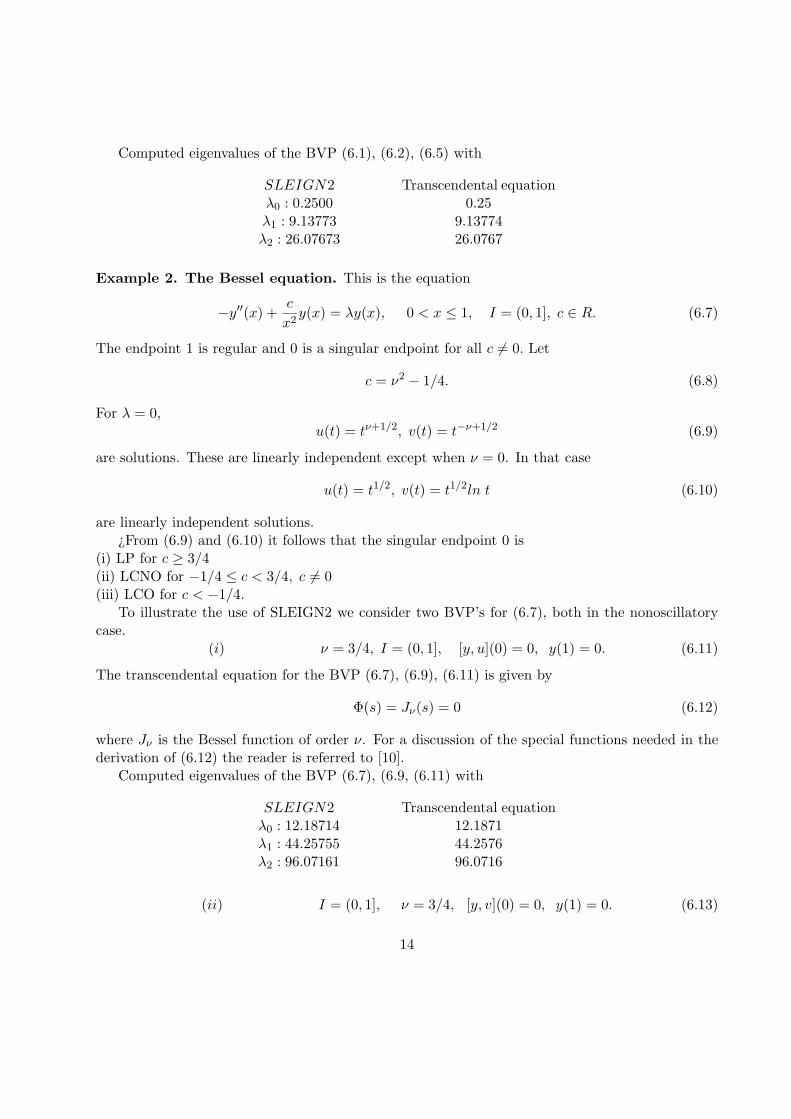
Example 2. The Bessel equation. This is the equation

−y′′(x) +c

x2y(x) = λy(x), 0 < x ≤ 1, I = (0, 1], c ∈ R. (6.7)

The endpoint 1 is regular and 0 is a singular endpoint for all c 6= 0. Let

c = ν2 − 1/4. (6.8)

For λ = 0,u(t) = tν+1/2, v(t) = t−ν+1/2 (6.9)

are solutions. These are linearly independent except when ν = 0. In that case

u(t) = t1/2, v(t) = t1/2ln t (6.10)

are linearly independent solutions.¿From (6.9) and (6.10) it follows that the singular endpoint 0 is

(i) LP for c ≥ 3/4(ii) LCNO for −1/4 ≤ c < 3/4, c 6= 0(iii) LCO for c < −1/4.

To illustrate the use of SLEIGN2 we consider two BVP’s for (6.7), both in the nonoscillatorycase.

(i) ν = 3/4, I = (0, 1], [y, u](0) = 0, y(1) = 0. (6.11)

The transcendental equation for the BVP (6.7), (6.9), (6.11) is given by

Φ(s) = Jν(s) = 0 (6.12)

where Jν is the Bessel function of order ν. For a discussion of the special functions needed in thederivation of (6.12) the reader is referred to [10].

Computed eigenvalues of the BVP (6.7), (6.9, (6.11) with

SLEIGN2 Transcendental equationλ0 : 12.18714 12.1871λ1 : 44.25755 44.2576λ2 : 96.07161 96.0716

(ii) I = (0, 1], ν = 3/4, [y, v](0) = 0, y(1) = 0. (6.13)

14

In this case the transcendental equation is

Φ(s) ≡ J−ν(s) = 0. (6.14)

For a discussion of the special functions needed to derive (6.14) see [10].Computed eigenvalues of the BVP (6.7), (6.9), (6.13) with

SLEIGN2 Transcendental equationλ0 : 1.12055 1.12044λ1 : 18.3540 18.3531λ2 : 55.3622 55.3603 .

Example 3. The Boyd equation. This is the equation, see [8],

−y′′(x)− 1xy(x) = λy(x), 0 < x ≤ 1, I = (0, 1]. (6.15)

The endpoint 1 is regular, and the endpoint 0 is singular and in the LCNO case. General solutionscan be obtained in terms of the confluent hypergeometric functions and are, see [8], [11],

Mk,1/2(x/k) Wk,1/2(x/k)

where k = k(λ) = (2is)−1, and M , W are the Whittaker functions. The solution kMk,1/2(x/k) isanalytic in both x and λ in all of C; hence (6.15) is nonoscillatory at 0. In this case it is easier touse maximal domain functions to determine the boundary conditions at zero rather than solutions.It can be checked that

u(x) = x, v(x) = 1− x ln(x), x ∈ I, (6.16)

are in ∆, the maximal domain and that

[u, v](x)→ −1 as x→ 0+. (6.17)

¿From this it follows [20] that 0 is a LC endpoint. Thus 0 is LCNO.Boundary conditions.

(i) I = (0, 1], [y, u](0) = 0, y(1) = 0. (6.18)

The transcendental equation for the BVP (6.15), (6.16), (6.18) is

Φ(s) = (2is)−1M(2is)−1,2−1(2is) = 0. (6.19)

There are infinitely many roots of (6.19) on the positive real axis s = σ > 0 (s = 0 is not aneigenvalue; this is the reason for the presence of the factor (2is)−1) and possibly a finite numberon the line s = iτ with τ > 0.

15

Computed eigenvalues of the BVP (6.15), (6.16), (6.18) are

SLEIGN2 Transcendental equationλ0 : 7.37399 7.3740λ1 : 36.33602 36.3360λ2 : 85.29258 85.2925λ3 : 154.09862 154.099λ4 : 242.70555 242.705

(ii) I = (0, 1], [y, v](0) = 0 y(1) = 0 . (6.20)

The transcendental equation for the BVP (6.15), (6.16), (6.20) is

Φ(s) = Γ(1− (2is)−1)W(2is)−1,1/2(2is) = 0. (6.21)

Again, there are infinitely many roots of (6.21) on the positive real axis s = σ > 0; and possibly afinite number on the positive imaginary axis s = iτ with τ > 0.

Computed eigenvalues of BVP (6.15), (6.16), (6.20) are

SLEIGN2 Transcendental equationλ0 : 0.984323 0.98432λ1 : 21.97069 21.9707λ2 : 62.12795 62.1281λ3 : 121.81338 121.813λ4 : 201.11951 201.120

In this example there is another method for obtaining the results of both BVP’s (i) and (ii)above.

It is shown in [2, Section 3] that the singularity at 0 of the Boyd equation (6.15) can be regu-larized at the expense of using quasi-derivatives and a weight function. Details of this regularizingtransformation are mentioned in [2, Section 4] with references to other relevant papers. The BVP(6.15), (6.16), (6.18) has the same eigenvalues as the following regular S-L problem in the weightedHilbert space L2((0, 1);w)

−(py′)′ + qy = λwy on [0, 1] = I (6.22)

(i)′ y(0) = 0 = y(1) (6.23)

wherep = r2, w = r2, q = −r2ln2, (6.24)

withr(x) = exp(−(xln(x)− x)) x ∈ [0, 1]. (6.25)

Note that p and w are continuous and positive on [0,1]; q is not bounded on [0,1] but q ∈ L(0, 1).Hence (6.22), (6.23), (6.24) is a regular S-L problem. (Although the eigenvalues of (6.22), (6.23),(6.24) are the same as those of (6.15), (6.16), (6.18) the eigenfunctions are not. However, the

16

eigenfunctions of the two problems are related to each other by a simple transformation, namelymultiplication by a function.)

This example, and others like it, which are regular according to the minimal conditions imposedby Definition 2.1 above, and yet have one or more coefficients which are unbounded at an endpoint,makes it desirable to have a computer eigenvalue routine which is effective in such cases. Forthis reason SLEIGN2 is designed to handle such problems, which in this paper are designated by“weakly regular” problems. Note that a weakly regular problem is a regular problem in the senseof Definition 2.1.

When applied to the weakly regular problem (6.22) and (6.23) SLEIGN2 computed the followingvalues

λ0 : 7.37418λ1 : 36.33650λ2 : 85.29278λ3 : 154.09987λ4 : 242.70728

which are seen to compare favorably with those values obtained in the singular problem (6.15) to(6.18).

Similarly the singular problem (6.15), (6.16), (6.20) has the same eigenvalues as the regularproblem (6.22), (6.24) with the boundary conditions

(ii)′ y(0) + (py′)(0) = 0, y(1) = 0. (6.26)

Again applying SLEIGN2 to this weakly regular problem yields the values

λ0 : 0.9847λ1 : 21.97142λ2 : 62.12913λ3 : 121.81473λ4 : 201.12811

which should be compared with those values obtained for the singular problem (6.15), (6.16) and(6.20).Example 4. The Sears-Titchmarsh equation. This is given by

−y′′(x)− e2xy(x) = λy(x), 0 ≤ x <∞, I = [0,∞). (6.27)

See [25,] [22].The substitution t = ex transforms (6.27) to

−(ty′(t))′ − ty(t) = λt−1y(t), 1 ≤ t <∞, I = [1,∞). (6.28)

In this form the equation (6.28) is a transformed version of Bessel’s equation (see Kamke [15, 1(a)of section C2.162 with the choice of parameters a = 1, m = 2, b = 1 and c = λ]). Solutions of(6.28) can be given in the form

Jis(t) and J−is(t).

17

For λ = −1/4 these solutions J±1/2(t) reduce to the elementary solutions

t−1/2 cos t and t−1/2 sin t on I.

It now follows that on [1,∞) (6.28) has the properties that the endpoint 1 is regular and theendpoint ∞ is LCO in L2((1,∞; t−1). We choose boundary condition functions u, v given by

u(t) = t−1/2(cos t+ sin t), v(t) = t−1/2(cos t− sin t). (6.29)

Boundary conditions.

(i) I = [1,∞), y(1) = 0, [y, u](∞) = 0. (6.30)

The transcendental equation for the BVP (6.28), (6.29), (6.30) is given by

Φ(s) =Jis(1) + J−is(1)

2 cos(isπ/2)= 0. (6.31)

The factor in the denominator of (6.31) prevents the spurious roots

s = i(2r + 1), r ∈ N0

from appearing. (Recall that J−n(z) = (−1)nJn(z). The numbers (i(2r+ 1))2 = −(2r+ 1)2, r ∈ N0

are NOT eigenvalues). Since the endpoint at ∞ is oscillatory the eigenvalues of this problem areunbounded below as well as above. Thus the equation (6.31) has infinitely many roots on thenonnegative real axis s = σ ≥ 0 and infinitely many roots on the positive imaginary axis s = iτwith τ > 0.

Here we define λ0 to be the first nonnegative eigenvalue and the others such that

...λ−2 < λ−1 < λ0 < λ1 < λ2 < ... .

(i) Computed eigenvalues of the BVP (6.28), (6.29) and (6.30) are

SLEIGN2 Transcendental equation

λ−2 : −12.2449 −12.2476λ−1 : −1.69345 −1.69336λ0 : 6.76010 6.76091λ1 : 17.83053 17.8354

(ii) I = [1,∞) y(1) = 0 [y, v](∞) = 0. (6.32)

The transcendental equation for (6.28), (6.29), (6.32) is given by

Φ(s) =Jis(1)− J−is(1)

2sin(isπ/2)= 0. (6.33)

18

Again, the factor in the denominator prevents the roots

s = i2r, r ∈ N0

from occurring; the numbers(i2r)2 = −4r2, r ∈ N0

are NOT eigenvalues; there are infinitely many positive and infinitely many negative eigenvalues.Computed eigenvalues of (6.28), (6.29), (6.32) are

SLEIGN2 Transcendental equationλ−2 : −20.2499 −20.2499λ−1 : −6.19488 −6.19343λ0 : 2.29382 2.29404λ1 : 11.96032 11.9682

Example 5. The BEZ equation. This is

−(xy′(x))′ − 1xy(x) = λy(x), 0 < x ≤ 1, I (0, 1]. (6.34)

The equation (6.34) is also a special case of a (transformed) version of the Bessel equation. SeeKamke [15, (1a) of section C2.162 with choice of parameters a = c = m = 1, b = λ] for details.Solutions of (6.34) can be expressed in terms of the Bessel functions

J+2i(2x1/2s) and J−2i(2x1/2s).

For λ = 0 these solutions reduce to the form

xi and x−i

and from these we obtain the elementary real solutions

u(x) = cos(ln(x)) and v(x) = sin(ln(x)), 0 < x ≤ 1. (6.35)

Thus the endpoint 0 is LCO and the endpoint 1 is regular.Boundary value problems.

(i) I = (0, 1], [y, u](0) = 0, y(1) = 0. (6.36)

The eigenvalues of the BVP (6.34), (6.35), (6.36) are characterized by the roots of the equation

Φ(s) = Γ(1 + 2i)s−2iJ2i(2s) + Γ(1− 2i)s2iJ−2i(2s) = 0. (6.37)

There are infinitely many roots of (6.37) of the form s = σ ≥ 0 and infinitely many of the forms = iτ with τ > 0; s = 0 is not a root.

19

Computed eigenvalues of (6.34), (6.35), (6.36) are

SLEIGN2 Transcendental equationλ−2 : −126.73 −126.727λ−1 : −5.42637 −5.4264λ0 : 4.39738 4.3976λ1 : 18.11879 18.1188λ2 : 37.91803 37.9181λ3 : 63.46119 63.4664

(ii) I = (0, 1], [y, v](0) = 0 y(1) = 0. (6.38)

The transcendental equation for the BVP (6.34), (6.35), (6.38) is given by

Φ(s) = Γ(1 + 2i)s−2iJ2i(2s)− Γ(1− 2i)s2iJ−2i(2s) = 0. (6.39)

This time s = 0 is a root of (6.39) and there are infinitely many positive roots s = σ > 0 andinfinitely many roots of the form s = iτ with τ > 0.

Computed eigenvalues of (6.34), (6.35), (6.38) are

SLEIGN2 Transcendental equationλ−3 : −19, 461.1λ−2 : −609.62λ−1 : −26.335 −26.3430λ0 : 0.0000 0.0000λ1 : 10.44857 10.4481λ2 : 27.28691 27.2868λ3 : 50.1425 50.0150λ4 : 78.36476 78.364λ5 : 112.19733 112.196

In this example SLEIGN2 could not reach λ−2 and λ−3 but it is likely that this difficulty was dueto machine capacity and could be removed with a larger computing facility.Example 6. The BEZ2 equation. If we take the BEZ equation (6.34) and move the LCsingularity from the origin 0 to the endpoints +1 and −1, and then bring the two transformedequations together we obtain

−((1− |x|)y′(x))′ − 11− |x|

y(x) = λy(x) − 1 < x < 1. (6.40)

Solutions of this equation are

J+2i(2(1− |x|)1/2s) and J−2i(2(1− |x|)1/2s);

all solutions y and their quasi-derivatives py′ (where p(x) = 1 − |x| (x ∈ (−1, 1))) are continuousat the origin 0; the classical derivative y′ may or may not be continuous at 0.

20

This example is LCO at both endpoints +1 and −1. Separated boundary conditons can beimposed at these endpoints, as in Example 5, by using the solutions when λ = 0 i.e.

u(x) = cos(ln(1− |x|) v(x) = sin(ln(1− |x|)) (x ∈ (−1, 1)). (6.41)

To illustrate the effectiveness of SLEIGN2 in the case of boundary value problems when bothendpoints are LCO, two sets of boundary conditions are considered. The eigenvalues have beencomputed by SLEIGN2 and are given below; we have not made use of the equivalent transcendentalequation but since the coefficients of the equation (6.40) are even about the origin 0 of (−1, 1), thechoice of both boundary conditions gives all eigenfunctions as even or odd. The odd eigenfunctionssatisfy y(0) = 0 and so also appear in one or other of the two boundary value problems (i) and (ii)of the BEZ equation in Example 5. Thus to obtain an independent check on the results for theBEZ2 equation reference should be made to the results of the previous example.

Boundary value problems

(i) I = (−1, 1) [y, v](−1) = [y, v](1) = 0 (6.42)

Computed eigenvalues are:

SLEIGN2 Transcendental equationλ−1 : −5.42635 −5.42636λ0 : 0.0000λ1 : 4.39755 4.39755λ2 : 10.16808λ3 : 18.11874 18.1188

(ii) I = (−1, 1) [y, v](−1) = [y, v](1) = 0 (6.43)

Computed eigenvalues are:

SLEIGN2 Transcendental equationλ−2 : −26.366 −26.3440λ−1 : −1.75422λ0 : 0.0000 0.000λ1 : 4.10963λ2 : 10.44811 10.4481

Example 7: The Latzko equation This is the differential equation

−((1− x7)y′(x))′ = λx7y(x) 0 ≤ x < 1 (6.44)

which has a celebrated history; it is associated with a heat conduction problem first studied byLatzko in 1921. For full details to the literature concerned with the study of this equation and anassociated boundary value problem see Fichera [12, Pages 43 to 45 and detailed references].

21

The differential equation (6.44) has a strong comparison with the Legendre equation (6.1). Theendpoint 0 is clearly regular; the endpoint 1 is singular since

∫ 10 (1 − x7)−1dx = ∞. To determine

the classification of 1 let λ = 0 when solutions are

1 and∫ x

0

11− t7

dt (x ∈ [0, 1)).

Now∫ x

0 (1− t7)−1dx ∼ K ln(1/(1− x)) as x → 1− for some K > 0. Thus both solutions are inL2(0, 1) and hence in the weighted space L2(0, 1; x7); hence endpoint 1 is in the LC case. Since 1is a solution on [0, 1) this endpoint is LCNO.

For boundary condition functions we can take

u(x) = 1 v(x) = ln(1/(1− x)) (x ∈ [0, 1)) (6.45)

noting that u is a solution, but v is a maximal domain function which is not a solution. A calculationshows that [u, v](1) = 7 6= 0 so that the pair {u, v} form a bases for boundary conditions at 1.

The boundary value problem considered by Fichera [12, Page 43] is equivalent to

(i) I = [0, 1) y(0) = 0 [y, u](1) = 0 (6.46)

This is not immediately clear since the Fichera problem [12, (1.11.12)] requires that limx→1− y(x)exist and is finite at 1. However it may be shown that this requirement is equivalent to the boundarycondition [y, u](1) = 0 of (6.46), i.e. y ∈ ∆ and [y, u](1) = 0 is equivalent to y′ ∈ L(0, 1) and isequivalent to y ∈ AC[0, 1]. This is a typical case in which a boundary value problem in appliedmathematics has to have a boundary condition interpreted in the Glazman-Krein-Naimark form;see [20, Chapter V].

Extended efforts have been made to find numerical approximations to the first few eigenvalues ofthe problem (6.46); see [12, Page 44]. Here we report only on the results of Scarpini [12, references95, 96]

8.721575 < λ0 < 8.727471128.2512 < λ1 < 152.4231 (6.47)208.3475 < λ2 < 435.0634

and the results of Durfee [12, reference 90]

λ0 = 8.72747λ1 = 152.423λ2 = 435.06 (6.48)λ3 = 855.68λ4 = 1414.1

22

When SLEIGN2 is applied to (6.46) the following results are obtained

λ0 = 8.7274702λ1 = 152.423014λ2 = 435.060768 (6.49)λ3 = 855.6817λ4 = 1414.12619.

Two comments are called for:(a) The comparison between the results (6.48) and (6.49) is impressive and consolidates both

the early work of Durfee and the effectiveness of SLEIGN2 .(b) Equally impressive is the comparison between (6.47) and (6.49). The upper bounds in (6.47)

are obtained by the method of orthogonal invariants, see [12], and it now appears likely that theseupper bounds are in fact numerical approximations in themselves to the respective eigenvalues. Itis of interest to ask if this result can be proved in general from the analysis in Fichera [12].

The second boundary value problem discussed here, but one not considered in Fichera [12] is(see (6.45) for boundary condition function v)

(ii) I = [0, 1) y(0) = 0 [y, v](1) = 0. (6.50)

When SLEIGN2 is applied to (6.50) the following results are obtained

λ0 = 11.44499λ1 = 110.55933λ2 = 1324.5611

(6.51)

It would be of great interest to compare these results with the corresponding result from themethod of orthogonal invariants.

Example 8: The Laplace tidal wave equation This important differential equation is discussedby Homer [14]; it has a long history as reflected in the references given in [14].

The complete form of the equation is

−(1− µ2

µ2 − τ2y′(µ))′ +

1µ2 − τ2

[s

τ(µ2 + τ2

µ2 − τ2) +

s2

1− µ2]y(µ)

= λy(µ) (−1 < µ < 1) (6.52)

where the physical parameters s and τ satisfy

s ∈ Z\{0} 0 < τ < 1. (6.53)

It is important to note that the equation (6.52) not only has singular endpoints but also interiorsingularities at ±τ . There is the additional interest, both for the analysis and for the application to

23

tidal wave theory, that the leading coefficient (1−µ2)/(µ2− τ2) changes sign at the interior points±τ , in view of (6.53).

There are no known explicit solutions of (6.52) in terms of special functions or contour integrals.In this example then there is no transcendental equation for the calculation of eigenvalues. Never-theless in view of the importance of the tidal wave equation for applied mathematics a considerableeffort has been extended to obtain numerical values for the eigenfunctions and eigenvalues of (6.52),when the equation is considered in the space L2(−1, 1). For details see [14] and the references givenin that paper.

Here we do not attempt to apply SLEIGN2 to the tidal wave equation in its complete form,since some limit-point singularities are involved, but we consider a particular differential equationwhich represents the nature of the interior limit-circle singularities of the general equation.

The differential equations is, see [14, Equations (3.3) and (3.4)]

−(1xy′(x))′ + (

k

x2+k2

x)y(x) = λy(x) (x ∈ (0, 1)) (6.54)

where the parameter k ∈ R and k 6= 0, i.e. k2 > 0. For convenience, as in [14], we have placed thesingularity at the origin.

With no explicit solutions for this equation we classify the singularity at 0 by looking at elementsof the maximal domain ∆, see [14, Pages 165 to 168]. A calculation show that

(i) x2 and x− 1k∈ ∆ (6.55)

(ii) [x2, x− 1k

] =1x

(x2 − 2x(x− 1k

))→ 2k6= 0 as x→ 0 + .

Thus the equation is LC at 0. Additionally a Frobenius analysis at 0 shows that there are solutionsof the form

∞∑n=0

anxn and x2

∞∑n=0

bnxn

in a neighborhood of the origin; see [14, Page 165]. Hence the equation is LCNO in L2(0, 1) and abasis for the boundary condition functions is

u(x) = x2 v(x) = x− 1k

(x ∈ (0, 1)). (6.56)

The outcome of an application of SLEIGN2 to the following two boundary values problems isgiven below:

(i) I = (0, 1] [y, u](0) = 0 y(1) = 0 (6.57)(ii) I = (0, 1] [y, v](0) = 0 y(1)0 (6.58)

24

(i) k = 1 λ0 : 30.39575λ1 : 102.4418

k = −0.5 λ0 : 24.4595λ1 94.1055

(ii) k = 1 λ0 : −1.58500λ1 : 42.1899λ2 : 127.6009

k = −0.5 Not able to obtain numbers reliableto more than one digit.

This tidal wave example has presented SLEIGN2 with a number of unusual difficulties which areunder investigation. We hope to report further on this example in a subsequent publication.

25

Comments on the examples.

1. Two boundary value problems are considered for each equation. For Examples 1, 2, and 3there is a ”special” boundary condition. This is the condition which determines the Friedrichsextension. It is condition (6.3) for Example 1, (6.11) for Example 2 and (6.18) for Example 3.For the first two examples this follows from the well known fact (see Niessen and Zettl [21])that the Friedrichs extension is determined by the principal solution boundary condition.In Example 3 this follows from the fact that the maximal domain function u in (6.16) isasymptotically the same as the principle solution Mk,1/2(x/k). In these three examples bothendpoints are nonoscillatory and consequently (see [21]) the minimal operator is boundedbelow and hence has a Friedrichs extension.

In Examples 4 and 5 one endpoint is oscillatory; Example 6 has both endpoints oscilla-tory. Consequently ([21]) the minimal operator is not bounded below. Therefore there is noFriedrichs extension in these three cases, i.e. there is no ”special” (”ausgezeichnete” is theword Friedrichs used) boundary condition.

Examples 7 and 8 follow the same pattern as Examples 1, 2 and 3; the special boundaryconditions are (6.46) and (6.57) respectively.

2. In Examples 1, 2, 7 and 8, SLEIGN rather than SLEIGN2 could be used to compute theeigenvalues for the Friedrichs boundary condition, but not for the other boundary conditions.For Examples 4, 5 and 6, SLEIGN2 must be used since SLEIGN is not designed to handlegeneral limit-circle boundary conditions.

3. We believe SLEIGN2 is the first general purpose S-L code capable of computing eigenvaluesin the oscillatory limit-circle case.

4. In giving the numerical results from SLEIGN2 for Examples 1 to 8 we have not attemptedto obtain precision results of the kind given in papers relating to SLEIGN; see for exampleBailey [3], Bailey, Garbow, Kaper, Zettl [5] and Marletta [19]. We have been concernedin this general paper to show that it is possible to offer an automatic computing code forSturm-Liouville boundary value problems in the limit-circle case and allow the user to selectboundary conditions. The results obtained and the comparison with earlier results or re-sults from transcendental equations, confirm our belief that SLEIGN2 is capable of fulfillingour objectives. When SLEIGN2 is made available in the public domain we shall also makeavailable more detailed numerical results which will indicate not only the scope, but also theprecision of this code.

References

[1] F. V. Atkinson. Discrete and continuous boundary value problems. (Academic Press; NewYork, 1964).

[2] F. V. Atkinson, W. N. Everitt and A. Zettl. Regularization of a Sturm-Liouville problem withan interior singularity using quasi-derivatives. Diff. and Int. Equations 1(1988), 213-212.

26

[3] P. B. Bailey. SLEIGN: an eigenfunction-eigenvalue code for Sturm-Liouville problems.SAND77-2044, Sandia Laboratories, Albuquerque (1978).

[4] P. B. Baily. Modified Prufer transformations. J. Comp. Phys. 29 (1978), 306-310.

[5] P. B. Bailey, B. S. Garbow, H. G. Kaper and A. Zettl. Eigenvalue and eigenfunction com-putations for Sturm-Liouville problems. ACM Trans. Math. Software (to appear)

[6] P. B. Bailey, B. S. Garbow, H. G. Kaper and A. Zettl. Algorithm XXX A FORTRANsoftware package for Sturm-Liouville problems. ACM Trans. Math. Software (to appear).

[7] P. B. Bailey, M. K. Gordon and L. F. Shampine. Automatic solution of the Sturm-Liouvilleproblem. ACM Trans. Math. Software, 4 (1978), 193-208.

[8] J. P. Boyd. Sturm-Liouville eigenvalue problems with an interior pole. J. Math. Physics,22(1981), 1575-1590.

[9] DO2KEF-NAG FORTRAN Library Routine Document.

[10] A. Erdelyi et al. Higher transcendental functions, Volumes I and II (McGraw-Hill; NewYork).

[11] W. N. Everitt, J. Gunson and A. Zettl. Some comments on Sturm-Liouville eigenvalueproblems with interior singularities. J. Appl. Math. Phys (ZAMP) 38(1987), 813-838.

[12] G. Fichera. Numerical and quantitative analysis (Pitman, London: 1978).

[13] C. T. Fulton. Expansions in Legendre functions Quart. J. Math (Oxford) (2) 33(1982), 215-222.

[14] M. S. Homer. Boundary value problems for the Laplace tidal wave equation. Proc. Roy. Soc.Lond. (A) 428(1990), 157-180.

[15] E. Kamke. Differentialgleichungen: Losungsmethoden und Losungen I: Gewohnliche Differ-entialgleichungen (Akademische Verlagsgesellschaft, Leipzig; 1959).

[16] T. Kato. Perturbation theory for linear operators (Second edition; Springer-Verlag, Heide-berg; 1980).

[17] A. M. Krall. Boundary value problems for an eigenvalue problem with a singular potential.J. Diff. Eq. 45(1982), 128-138.

[18] P. Linz. A critique of numerical analysis. Bull. Amer. Math. Soc. 19(1988), 407-416.

[19] M. Marletta. Numerical tests of the SLEIGN software for Sturm-Liouville problems. ACMTrans. Math. Software (to appear).

[20] M. A. Naimark. Linear differential operators, Volume II. (Ungar, New York; 1968).

27

[21] H.- D. Niessen and A. Zettl. Singular Sturm-Liouville problems; the Friedrichs extensionand comparison of eigenvalues (Pre-print 1990).

[22] D. B. Sears and E. C. Titchmarsh. Some eigenfunction formulae. Quart. J. Math. (Oxford)(2)1(1950), 165-175.

[23] I. J. Thompson and A. R. Barnett. COULCC: A continued-fraction algorithm for Coulombfunctions of complex order with complex arguments. Computer Physics Communications36(1985), 363-372.

[24] I. J. Thompson and A. R. Barnett. Coulomb and Bessel functions of complex argument andorder. Journal of Computational Physics 64(1986), 490-509.

[25] E. C. Titchmarsh. Eigenfunction expansions associated with second order differential equa-tions, Volume I (Clarendon Press, Oxford; 1962).

[26] J. Weidmann. Spectral theory of ordinary differential operators, Lecture Notes in Mathemat-ics 1258 (Springer-Verlag, Heidelberg; 1987).

28