COMPUTER SCIENCE - Wikispaces Specifications...Computer Science: Specifications ... Flow chart symbols and pseudocode ... Trace Tables for Desk Checking, Testing and Debugging

Computer Science: Specifications booklet (updated September 2011 for 2012) 1

COMPUTER SCIENCE

Specifications booklet 2012

This booklet supplements the Computer Science course and will be reviewed as required. It is to be used in conjunction with the: • course syllabus • scope and sequence document

2008/22533v6


Copyright © Curriculum Council, 2009–2010 This document—apart from any third party copyright material contained in it—may be freely copied, or communicated on an intranet, for non-commercial purposes by educational institutions, provided that it is not changed in any way and that the Curriculum Council is acknowledged as the copyright owner. Teachers in schools offering the Western Australian Certificate of Education (WACE) may change the document, provided that the Curriculum Council’s moral rights are not infringed. Copying or communication for any other purpose can be done only within the terms of the Copyright Act or by permission of the Curriculum Council. Copying or communication of any third party copyright material contained in this document can be done only within the terms of the Copyright Act or by permission of the copyright owners.

Disclaimer Any resources such as texts, websites and so on that may be referred to in this document are provided as examples of resources that teachers can use to support their learning programs. Their inclusion does not imply that they are mandatory or that they are the only resources relevant to the course.


Contents Unit 3B – Networks .......................................................................................................................................... 4

Communications protocols and standards ....................................................................................................................... 4 Unit 3A – Systems analysis and development ............................................................................................. 4

RAID ................................................................................................................................................................................. 4 Snapshot imaging ............................................................................................................................................................. 4 Platform virtualisation ....................................................................................................................................................... 4

Unit 2A/3A – Systems analysis and development ........................................................................................ 6 Systems Development Life Cycle (SDLC) ........................................................................................................................ 6

Unit 3A – Systems analysis and development ............................................................................................. 6 Gantt Chart ....................................................................................................................................................................... 6 Program Evaluation Review Technique (PERT) Analysis ................................................................................................ 7

Unit 2B – Programming .................................................................................................................................. 8 Units 1B, 2B, 3B – Programming ................................................................................................................... 9 Unit 1B – Programming ................................................................................................................................ 10 Unit 2B – Program Components and Simple Algorithms .......................................................................... 11

Flow chart symbols and pseudocode ............................................................................................................................. 11 Unit 2A – Developing software ..................................................................................................................... 17 Unit 2B – Programming ................................................................................................................................ 18

Trace Tables for Desk Checking, Testing and Debugging ............................................................................................. 18 Expanded method .......................................................................................................................................................... 18

Unit 3B – Programming ................................................................................................................................ 19 Trace Tables for Desk Checking, Testing and Debugging ............................................................................................. 19 Condensed method ........................................................................................................................................................ 19

Unit 2B – Modules ......................................................................................................................................... 20 Unit 3B – Programming ................................................................................................................................ 20

Program Constructs, Structured Programming, Algorithmic and Programming Techniques ......................................... 20 Algorithmic and programming techniques including documentation .............................................................................. 20 Structured programming using modularisation and parameter passing ......................................................................... 20

Unit 3B – Programming ................................................................................................................................ 21 Structured Programming Using Structure Charts ........................................................................................................... 21 Structured Programming Using Functions ..................................................................................................................... 21 Fundamentals of Data Structures ................................................................................................................................... 22

Arrays (one-dimensional) ........................................................................................................................................... 22 Records ...................................................................................................................................................................... 22

Testing and Debugging .................................................................................................................................................. 23 Condensed method ........................................................................................................................................................ 23

Unit 2A – Systems analysis and development ........................................................................................... 24 Data Flow Diagrams (DFD) ............................................................................................................................................ 24 Context diagram ............................................................................................................................................................. 24 Levelled data flow diagrams ........................................................................................................................................... 25

Unit 3A – Systems analysis and development ........................................................................................... 27 Levelled Data Flow Diagrams ........................................................................................................................................ 27 Example – Level 1 DFD for Process 3.0 Compile Monthly Newsletter .......................................................................... 27

Managing data ............................................................................................................................................... 28 Unit 2A – Managing data ............................................................................................................................... 29

Introduction to Entity Relationship Diagrams ................................................................................................................. 29 Symbols and characteristics ........................................................................................................................................... 29

Unit 3A – Managing data ............................................................................................................................... 30 Keys ............................................................................................................................................................................... 30 Entity Relationship Diagrams ......................................................................................................................................... 30

Unit 3A – Managing data ............................................................................................................................... 32 Unit 3A – Managing Data – Normalisation .................................................................................................. 33 Normalisation to Third Normal Form (3NF) ................................................................................................ 35

Another Normalisation example ..................................................................................................................................... 36 Purpose The elaborations in this booklet are to be used in conjunction with the syllabus. The elaborations only cover a portion of the course and are intended to:

• show the required breadth and depth of treatment of some concepts (e.g. virtualisation) • demonstrate how tools such as ERDs and DFDs should be used when answering exam

questions.


Unit 3B – Networks Communications protocols and standards (Refer to syllabus content on p. 21) Unit 3B provides an overview of the four layers within TCP/IP. Application Transport Internet Link

Unit 3A – Systems analysis and development (Refer to syllabus content on p. 17) RAID Is an acronym for Redundant Array of Independent Devices. This technology divides and replicates data among multiple device drives. There are numerous types of RAID. Level 0, 1 and 10 are referred to in the syllabus. Use the following links to access more information: http://searchstorage.techtarget.com/definition/RAID http://en.wikipedia.org/wiki/RAID Unit 3A – Systems analysis and development (Refer to syllabus content on p. 17) Snapshot imaging Is making a virtual copy of a device or file system. Snapshots imitate the way a file or device looked at the precise time the snapshot was taken. It is not a copy of the data, only a picture in time of how the data was organised. Snapshots can be taken at a scheduled time and provides a consistent view of a file system or device for a backup and recovery program to work from. Unit 3A – Systems analysis and development (Refer to syllabus content on p. 17) Platform virtualisation A virtual machine is a tightly isolated software container that can run its own operating systems and applications as if it were a physical computer. A virtual machine behaves exactly like a physical computer and contains it own virtual (i.e. software allocated portion of) CPU, RAM, hard disk and network interface card (NIC). An operating system can’t tell the difference between a virtual machine and a physical machine, nor can applications or other computers on a network. Even the virtual machine thinks it is a “real” computer. Nevertheless, a virtual machine is composed entirely of software and contains no hardware components whatsoever. Un-virtualised Machine Virtualised Machine


Benefits of virtualisation include: • cost savings due to fewer physical machines and the maintenance of these • energy savings as fewer physical machines means less power and air-conditioning needed • faster application and service delivery • higher levels of business continuity as a virtual machine can be moved to another physical

machine to provide additional capacity or overcome hardware issues There are many types of virtualisation:

• Server Virtualisation is where multiple logical servers are hosted on the one physical computer. Each server has its own operating system. Hence you can have a Windows 2008 Server and a Linux Server running on the same piece of hardware. This saves on the purchase of new equipment and also allows easier management of servers because they are on the one physical machine. Savings are also made on the cost of electricity for the server and air conditioning, as well as the cost of floor space.

• PC Virtualisation is where a single physical computer simultaneously runs multiple virtual PCs, each with its own operating system and suite of applications. Users can run different applications, such as software for a PC and a Mac, without having to switch machines. For example, if VMWare Fusion is installed on a Mac then the user can install Windows and Windows applications. This enables the user to switch between the Windows and Mac environments without needing to reboot. VMWare Player can be used on a PC so that different operating systems (e.g. Ubuntu, Chrome OS) can be used. For example, a system running Linux as the operating system can also run Windows applications if the Wine software is used.

• Desktop Virtualisation is the centralisation of applications at a data centre. This makes systems easier to manage. Initially desktop virtualisation was similar to terminal services such as Citrix where servers ran the applications and gave users remote access. All the user’s PC did was present the updated screen display and permit input via keyboard and mouse. Desktop virtualisation, on the other hand, is a new way of delivering the individual PC environment to the computer being used by the user. The servers host an entire desktop environment specific to each user. It is ideal for workers who move between machines or who work remotely.

• Storage Virtualisation is where many physical storage devices appear to the user as a single logical storage device.

See http://www.vmware.com or http://www.virtualbox.org/ for further details of some solutions.


Unit 2A/3A – Systems analysis and development (Refer to syllabus content on p. 13 and p. 17) Systems Development Life Cycle (SDLC) Different reference books may include slightly different versions of the SDLC. The stages that have been agreed on for this course are included below. Stages of the systems development life cycle (SDLC)

Preliminary analysis problem definition feasibility study

Analysis model of current system requirements of new system

Design logical and physical design

Development hardware and software acquisition construction and testing

Implementation change-over methods: direct cut, phased, pilot, parallel

Evaluation and maintenance performance evaluation fault finding and correction

Unit 3A – Systems analysis and development Gantt Chart The Gantt Chart shows the work breakdown structure (list of tasks with duration) and the relationship between the tasks. In the example below, most tasks have a Finish-Start relationship which indicates that a task must be completed before the next related task can commence. However, tasks 4 and 5 have a Start-Start relationship as they can be done at the same time.


Program Evaluation Review Technique (PERT) Analysis A Program, Evaluation, and Review Technique (PERT) analysis is used to determine a realistic duration for tasks, by taking into account optimistic, expected, and pessimistic duration estimates. An explanation of the PERT chart below is as follows:

• Order of tasks – 1–5 • Order of tasks – 6–10 • Branching 1, 2 and 3 • Branching 3, 4 and 5 • Branching 8, 9 and 10 • Duration/Time 1–5 • Duration/Time 6–10


Unit 2B – Programming (Refer to syllabus content on p. 15) Number systems Students should recognise decimal, binary and hexadecimal numbers and explain their purpose and use in computing. Number System Base Example Purpose Use Decimal 10 74 Binary 2 01001010 Hexadecimal 16 4A Specifying colours (e.g. HTML)

Assembly language programming Students should be able to understand the reasons for conversion from decimal to binary. Examples are shown below: Decimal to binary calculation Division method

Divide Technique 2 197

98 1 49 0 24 1 12 0 6 0 3 0 1 1 0 1

Subtraction method

197 Remainder 128 197-128 69 1

64 =69-64 5 1 32 0 16 0

8 0 4 =5-4 1 1 2 0 1 =1-1 0 1

Alternative subtraction method 27 26 25 24 23 22 21 20

128 64 32 16 8 4 2 1 197-128 69-64 5-4 1-1

1 1 0 0 0 1 0 1 Encoding Students should be able to explain the limitations of ASCII (American Standard Code for Information Interchange) as a 7 bit coding scheme (128 values only) and the benefits of Unicode as a 16 bit coding scheme. Students should be able to use an ASCII lookup table. Any required tables will be provided in an exam question.


Units 1B, 2B, 3B – Programming Overview Units 1B, 2B and 3B progressively develop knowledge about computer languages and skills in designing, creating, modifying, testing, evaluating and documenting programs. Unit 1B (Refer to syllabus content on p. 11) Program components require students to be able to identify inputs, processing and outputs. IPO charts will be used to organise this and interface designs will be planned. When using a simple programming language, students will not be required to write code. They will create programs by recording macros or using interactive drag and drop languages. They will then identify the components that have been created and inspect and edit the code. Unit 2B (Refer to syllabus content on p. 15) Program components and constructs focuses on simple algorithms using sequence, selection and repetition. These algorithms will be developed using flow charts (a graphical method) and pseudocode (structured English). Students will write, compile, interpret, test and debug code using procedural type programming. It is recommended that the language chosen includes a visual interface. Unit 3B (Refer to syllabus content on p. 20) Programming constructs and structured programming extend to more complex algorithms using modularisation and parameter passing, and one-dimensional arrays. These algorithms will be developed using pseudocode. External exam questions at Stage 3 will represent algorithms in pseudocode. Students will where appropriate to the programming language used, write, compile, interpret, test and debug code using procedural type programming. It is recommended that the language chosen includes a user interface. Recommended programming languages for Stage 1 are • Scratch • Alice • Macros––VBA, application specific macros, scripting languages, Unix Bash, Applescript,

Automator scripts.

Recommended programming languages for Stages 2 and 3 are • Visual Basic • Pascal • Python • PHP • Java • C# Review of these recommended languages will be on an ongoing basis.


Unit 1B – Programming (Refer to syllabus content on p. 11) Simple programming languages may involve: 1. creating programs through the use of either:

• recording macros in application programs such as Word, Excel and Automator OR • interactive drag and drop programs such as Scratch.

2. identifying components of the program by either: • inspecting code syntax for macros and making changes such as the size or font OR • recognising and using drag and drop components.

Program design using Input, Processing, Output (IPO) charts There are a number of ways that IPO charts can be set out, but the simple format below will be adopted. This requires the student to identify any inputs, the processing that will take place and the outputs required.

Input Processing Output • number of hours worked • hourly rate • tax rate

• calculate gross pay • calculate tax payable • calculate net pay

• gross pay • tax payable • net pay

Word Macros Tutorial on creating and editing Word Macros–http://www.officeletter.com/favtips/wordmacros.html Scratch programming language Freeware, downloadable from http://scratch.mit.edu/ Getting Started Guide, project ideas and online help are available. Simple to use drag and drop programming that introduces programming constructs and components. Tutorials and information on using Scratch, available from kidsprogramming.pbwiki.com Alice programming language Freeware, downloadable from http://www.alice.org/ Demonstration videos and tutorials are available. Simple to use drag and drop programming that introduces programming constructs and components.


Unit 2B – Program Components and Simple Algorithms (Refer to syllabus content on p. 15) Flow chart symbols and pseudocode

Symbol Meaning

Terminal: begin and end

Input or output

Process: the description of an action or process

Decision: one line comes in at the top and two lines leave it

Sub-program or module: a portion of code that performs a particular task. The Stage 2 syllabus does not include modules, but modular code should be encouraged as early as possible, as this promotes efficiency of code.

Sequence The instructions are processed in order.

Flowchart Pseudocode

Input (Num1) Input (Num2) Product ← Num1 * Num2 Output (Product)

OR Read (Num1) Read (Num2) Product ← Num1 * Num2 Write (Product)

Note: Read and Write can be used in place of Input and Output

Enter Num1

Enter Num2

Product = Num1 * Num

End

Print Product

Begin


Selection A condition is tested to determine which branch or path is followed.


One way selection If condition then

Input (Age) If Age >= 18 then

Output (‘Entrance allowed’) End If

Two-way selection If condition then .. else

Input (Age) If (Age >= 16) and (Age <= 65) then

Price ← 35 Else

Price ← 20 End If Output (‘The cost will be $’, Price)

Enter Age

Age >=18

true

Print ‘Entrance allowed.’

Begin

End

false

Enter Age

Age >=16 and Age <= 65?

true

Begin

End

false

Set Price to 35 Set Price to 20

Print ‘The cost will be $’ Price


Selection (continued) A condition is tested to determine which branch or path is followed.


Multi way selection (Case) Input (Age) Case Age of

< 4 : Fare ß 0 < 16 : Fare ß 5 < 60 : Fare ß 10 >= 60 : Fare ß 7

End Case Output (‘The cost of the trip will be $’, Fare)

Enter Age

CASE Age

Begin

End

<4

Set Fare to 0

Print ‘The cost of the trip will be $’ Fare

Set Fare to 5

Set Fare to 10

Set Fare to 7

<16 <60 >=60


Repetition also commonly called iteration or looping Repeating an action or series of actions a number of times. FOR: Fixed or counted loop This loops or repeats a counted or fixed number of times. The number of repetitions is known when the loop begins. Flow chart Pseudocode

TotalScore ← 0 For Batsman ß 1 to 11

Input (Score) TotalScore ß TotalScore + Score

End For Output (TotalScore)

Begin

Set TotalScore to 0

End

Enter Score

Set Batsman to 1

Batsman < = 11

Add Score to TotalScore

False

Increase Batsman by 1

Print TotalScor

e


While: test first or pre-test loop This loops a variable number of times. The number of repetitions is not known when the loop begins. This is tested before the loop is entered—test first—it is possible that the loop is executed zero times. Flow chart Pseudocode

TotalScore ← 0 Continue ← ‘Y’ While Continue = ‘Y’

Input (Score) TotalScore ß TotalScore + Score Input (Continue)

End While Output (TotalScore)

Begin

Set TotalScore to 0

End

Enter Score

Set Continue to ‘Y’

Continue = ‘Y’


true

false

Enter Continue

Print TotalScor

e


Repeat ... Until: test last of post-test loop This loops a variable number of times. The number of repetitions is not known when the loop begins. This is tested at the end of the loop—test last—and therefore must be executed at least once. Flow chart Pseudocode

TotalScore ← 0 Repeat

Input (Score) TotalScore ← TotalScore + Score Input (Continue) Until Continue = ‘N’ Output (‘Total score is ‘, TotalScore)

Repeat

Output (‘Enter your age in years’) Input (Age)

Until (Age > 0) and (Age <120) Output (‘Valid age entered’)

Begin

End

Print ‘Enter your age in years’

(Age > 0) and (Age <120)

true

false

Enter Age

Print ‘Valid age entered.’


Begin

End

Enter Score

Continue = ‘N’

true

false

Enter Continue

Print ‘Total score is’,

TotalScore

Set TotalScore to 0


Unit 2A – Developing software (Refer to syllabus content on p. 15) Developing software for a computer-based system involves: Knowledge • purpose and function of software to operate a computer system

§ operating systems § utility software

o file compression o defragmenter o anti-virus o anti-malware

• application software • requirements for software licensing

§ Freeware § Open source § Shareware

Skills • develop a system solution using the Software Development Cycle (SDC)

§ state the problem § plan and design § develop § test § evaluate

• software development requirements § user needs § user interface


Unit 2B – Programming (Refer to syllabus content on p. 15) Trace Tables for Desk Checking, Testing and Debugging The correctness of an algorithm should be checked before coding begins. Trace tables provide a formal method for tracing the logic of an algorithm. A set of data values (test data) is chosen to test all paths within the algorithm. All variables, constants and formal parameter values need to be represented. Below is a trace table of the following pseudocode using the data values [2, 3, 6, 5, 7, 999].

Module DisplayLargestNumber 1 Largest ß 0 2 Input (Number) 3 Repeat 4 If Number > Largest then 5 Largest ß Number 6 End If 7 Input (Number) 8 Until (Number = 999) 9 Output (‘The largest number is ‘, Largest) End Module

Expanded method Line Largest Number Number >

Largest Number =

999 Output

1 0 2 2 4 TRUE 5 2 7 3 8 FALSE 4 TRUE 5 3 7 6 8 FALSE 4 TRUE 5 6 7 5 8 FALSE 4 FALSE 7 7 8 FALSE 4 TRUE 5 7 7 999 8 TRUE 9 The largest number is 7

Lines 3 to 8 are a Repeat—Until loop, line 8 is the condition (test LAST) which will repeat the loop until this is TRUE. Lines 4 to 6 are an If statement. If the condition in line 4 is TRUE, then line 5 is processed, otherwise line 5 is skipped.


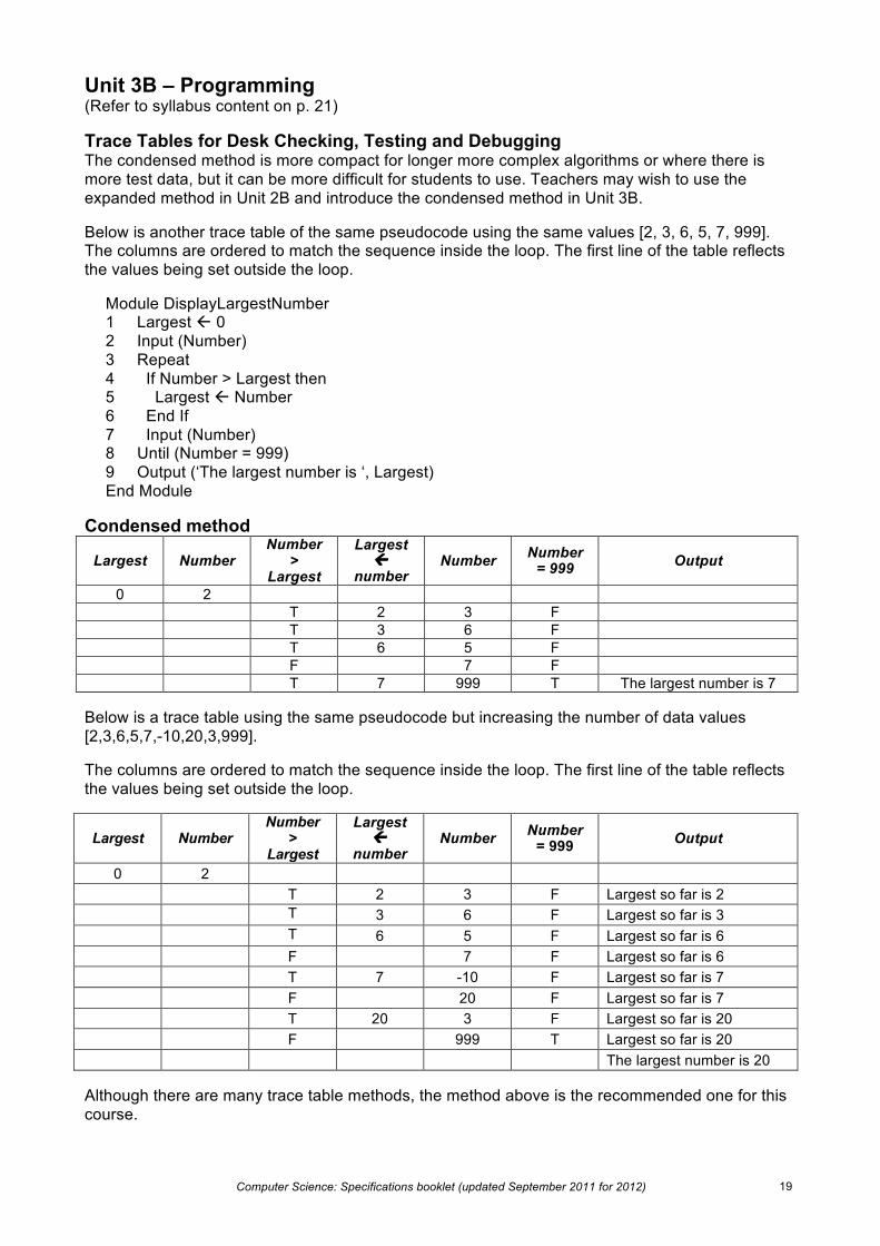
Unit 3B – Programming (Refer to syllabus content on p. 21) Trace Tables for Desk Checking, Testing and Debugging The condensed method is more compact for longer more complex algorithms or where there is more test data, but it can be more difficult for students to use. Teachers may wish to use the expanded method in Unit 2B and introduce the condensed method in Unit 3B. Below is another trace table of the same pseudocode using the same values [2, 3, 6, 5, 7, 999]. The columns are ordered to match the sequence inside the loop. The first line of the table reflects the values being set outside the loop.

Module DisplayLargestNumber 1 Largest ß 0 2 Input (Number) 3 Repeat 4 If Number > Largest then 5 Largest ß Number 6 End If 7 Input (Number) 8 Until (Number = 999) 9 Output (‘The largest number is ‘, Largest) End Module

Condensed method

Largest Number Number

> Largest

Largest ß

number Number Number

= 999 Output

0 2 T 2 3 F T 3 6 F T 6 5 F F 7 F T 7 999 T The largest number is 7

Below is a trace table using the same pseudocode but increasing the number of data values [2,3,6,5,7,-10,20,3,999].

The columns are ordered to match the sequence inside the loop. The first line of the table reflects the values being set outside the loop.

Largest Number Number

> Largest

Largest ß

number Number Number

= 999 Output

0 2 T 2 3 F Largest so far is 2 T 3 6 F Largest so far is 3 T 6 5 F Largest so far is 6 F 7 F Largest so far is 6 T 7 -10 F Largest so far is 7 F 20 F Largest so far is 7 T 20 3 F Largest so far is 20

F 999 T Largest so far is 20 The largest number is 20

Although there are many trace table methods, the method above is the recommended one for this course.


Unit 2B – Modules In Unit 2B students design and write code segments that may be modularised. However, they are not expected to pass parameters between modules. Unit 3B – Programming (Refer to syllabus content on p. 20) Program Constructs, Structured Programming, Algorithmic and Programming Techniques Pseudocode concepts for program design from Unit 2B are also required for Unit 3B. Algorithmic and programming techniques including documentation Algorithmic and programming techniques from Unit 2B are also required for Unit 3B. Internal documentation includes: the use of comments; meaningful identifiers for constants, variables and module names; and code layout with appropriate use of indentation and white space. Structured programming using modularisation and parameter passing In Unit 3B students design and write modularised code segments that pass parameters between the modules. Module examples Module CalculatePay (CRate, CHours, CPay)

CPay ← CRate * CHours End CalculatePay Module CalculateTax (TPay, TTax)

YearlyPay ← TPay * 52 Case YearlyPay of

<= 6000 : YearlyTax ← 0 <= 30000 : YearlyTax ← (YearlyPay – 6,000) * 0.15 <= 75000 : YearlyTax ← 3600 + (YearlyPay –30,000) * 0.3 <= 150000 : YearlyTax ← 17100 + (YearlyPay – 75,000) * 0.4 > 150000 : YearlyTax ← 47100 + (YearlyPay – 150,000) * 0.45

End Case TTax ← YearlyTax / 52

End CalculateTax Calling the modules

Module Main Input (Rate) Input (Hours) Call CalculatePay (Rate, Hours, Pay) Call CalculateTax (Pay, Tax) NettPay ← Pay - Tax Output (NettPay)

End Main

• The parameters CRate, CHours and CPay (used in the module) are referred to as formal parameters whereas the parameters Rate, Hours and Pay (used when the module is called) are referred to as the actual parameters.

• The parameters, Rate and Hours, are sent to the module CalculatePay and the calculated pay is returned through the Pay parameter.

• The parameters, CRate and CHours, are value parameters that receive a value, but do not return a changed value.


• The parameter, CPay, is a variable (pass by reference) parameter as it returns a value to the calling module.

• In module CalculateTax, TTax is a variable (pass by reference) parameter that returns a value and TPay is a value parameter that receives a value, but does not return a changed value.

Unit 3B – Programming (Refer to syllabus content on p. 20) Structured Programming Using Structure Charts Unit 3B structure charts represent modules graphically. The data parameters passed between modules are included.

Rate and Hours are parameters that send a value to the module, but do not return any value. Two-way parameters pay and tax would be variable parameters. This indicates that any changes made to the values are passed back to the calling module.

The structure chart is showing the actual parameters from Module Main, not the formal parameters shown in Module CalculatePay and Module CalculateTax. Unit 3B – Programming (Refer to syllabus content on p. 20) Structured Programming Using Functions Function example

Function PayCalc (PRate, PHours) PayCalc ← PRate * PHours

End Function Using the function in a calculation and as an output

Module Main Input (Rate) Input (Hours) Output (PayCalc(Rate, Hours)) Call CalculateTax(Tax, Pay) NettPay ← PayCalc – (Tax) Output (NettPay)

End Main A function is a special type of module that: • receives data through its parameters and returns a single value through the function name. In

the above example values are received through Rate and Hours and the calculated result is returned through the function name PayCalc

• has no input or output statements • can be used in a calculation, assignment statement or output statement.

Main

CalculateTax CalculatePay

Rate, Pay, Hours

Pay

Pay, Tax

Tax


It is generally preferable for efficiency of code to use a function (that does not alter the parameters that are passed into it) to return a value. Where possible it is preferable to pass a parameter into a module and alter that parameter within that module. Although it is best to pass back the result as the returned value rather than alter one of the parameters, it is not always possible. However, it does make for more readable code and is good coding practice. Unit 3B – Programming (Refer to syllabus content on p. 20) Fundamentals of Data Structures Arrays (one-dimensional) The first element of an array a [ ] is always referred to as [0], the second as a [1] and so forth. Array pseudocode examples Initialising an array with zeros

For Student ← 0 to 24 MarksList[Student] ← 0 End For

Reading data into an array

For Student ← 0 to 24 Input (MarksList[Student]) End For

Displaying all the data from an array

For Student ← 0 to 24 Output (MarksList[Student]) End For

Records Record pseudocode examples Record structure

StudentData Firstname Surname DateOfBirth Phone

Reading data into the student record Input (StudentData.Firstname) Input (StudentData.Surname) Input (StudentData.DateOfBirth) Input (StudentData.Phone)

Displaying data from the student record

Output (StudentData.Firstname) Output (StudentData.Surname) Output (StudentData.DateOfBirth) Output (StudentData.Phone)


Unit 3B – Programming (Refer to syllabus content on p. 20) Testing and Debugging The correctness of an algorithm should be checked before coding begins. Trace tables provide a formal method for tracing the logic of an algorithm. A set of data values (test data) is chosen to test all paths within the algorithm. • All variables, constants and formal parameter values need to be represented. • Any data structure (such as an array or record) should be represented separately to the table

of simple data types, so that changing values can be represented more easily. Condensed method In Unit 3B this condensed method is more compact for longer more complex algorithms or where there is more test data, but it can be more difficult for students to use. Below is a trace table of the following pseudocode using the data values [2,3,6,5,7,-10,20,3,999].

Module DisplayLargestNumber Largest ß 0 Input (Number) Repeat If Number > Largest then Largest ß Number End if Output (‘Largest so far is ‘, Largest) Input (Number) Until (Number = 999) Output (‘The largest number of all is ‘, Largest)

The columns are ordered to match the sequence inside the loop. The first line of the table reflects the values being set outside the loop.

Number > Largest Largest Output Number Number = 999

0 2 TRUE (2 > 0) 2 Largest so far is 2 3 FALSE TRUE (3 > 2 ) 3 Largest so far is 3 6 FALSE TRUE (6 > 3) 6 Largest so far is 6 5 FALSE FALSE (5 > 6) Largest so far is 6 7 FALSE TRUE (7 > 6) 7 Largest so far is 7 -10 FALSE FALSE (-10 > 7) Largest so far is 7 20 FALSE TRUE (20 > 7) 20 Largest so far is 20 3 FALSE FALSE (3 > 20) Largest so far is 20 999 TRUE

The largest number is 20


Unit 2A – Systems analysis and development (Refer to syllabus content on p. 13) Data Flow Diagrams (DFD) These conventions are based on the DeMarco/Yourdan symbols. See http://yourdon.com/strucanalysis/wiki/index.php?title=Chapter_9 Context diagram The context diagram is the top level of a set of hierarchically related diagrams that form a set that decomposes a system into successively finer detail with each move down the diagram set. This diagram represents the system being modelled as a single circle interacting with external entities. The emphasis of this diagram is to identify the boundary of the system. The name inside the single circle representing the system should describe the system being modelled. The symbols used are:

the system is represented as a circle

represents the flow of data between the system and the external entities

an organisation or person that provides data to the system or receives data from the system

Example – context diagram for social club system

NB – links in data flow names have been deleted. The circle is a representation of the system boundary. The system boundary defines what is inside and outside the system. Deciding on which side objects lie is an important consideration. Is a particular object part of the system being considered, and hence invisible inside the circle, or is it really outside the system’s considerations and therefore an external item supplying data, or taking information from the system? Notice that data stores or files must never appear in a context diagram. They are part of the system and are therefore inside the circle.

System

EXTERNAL

ENTITY

SOCIAL CLUB

SYSTEM

MEMBER

SOCIAL CLUB COMMITTEE

LOCAL

NEWSPAPER

member details

details confirmation

coming activities description

planned activity details

advertisement details


Levelled data flow diagrams A level 0 data flow diagram shows additional detail. It should show all external entities. The processes are numbered, but do not indicate sequence. Data stores are shown. All data flows are shown (between entity and process, between process and process, between process and data store). In the level 0 data flow diagram, the same total number of inflows and outflows (and external entities) must exist as in the context diagram, and these should have the same names as in the context diagram. The symbols used are: External entities: (sources or sinks): These are any organisation or person

that provides data to the system or receives data from the system. • They exist outside of the system. • An external entity can be both a source and a sink. • They should be named in the singular as a person, place or thing.

Processes: These are actions taking place that transform inputs into outputs. • They must always have at least one inflow and one outflow. • They should be named with an active verb associated with a noun or

very short phrases of that type, reflecting what transformation the process is making to the data passing through it.

• The numbering of a process does not indicate timing or sequence. • The data flowing out of a process should differ from that going in.

(e.g. payment cheque details goes in and cancelled cheque details comes out of an enter cheque transaction process.)

bookings file

Data stores: (files, repositories of data or temporary data stores) These store data used within a system. • They cannot transform data, and must usually contain at least one

inflow and one outflow. • A data store’s identifier should be a noun reflecting the data it contains

and not its physical nature e.g. bookings file NOT sorted magnetic tape file.

Data flows: These vectors indicate the data being transferred (not physical objects) e.g. invoice details not invoice. • They should connect at each end directly to their source and destination

with only one arrowhead. Sometimes in order to simplify a diagram, an entity or data store requires duplication. Each of the duplicated objects should contain a diagonal line in the bottom corner as shown below:

Timetables Bank Timetables Bank

1.0 Update

pay details

LIBRARY

invoice details


Example – Level 0 DFD for the social club system

Any similar information that data flows carry are resolved in the data dictionary. The number of processes that are in the level 0 data flow diagram depend on the number of major processes described.

1.0 Add new member

MEMBER

SOCIAL CLUB COMMITTEE

LOCAL

NEWSPAPER

member details

details confirmation

planned activity details

advertisement details

2.0 Add activity

4.0 Create

advertisement

3.0 Compile monthly

newsletter

new member details

all member details

new planned activity details

upcoming activities details


Members

Activities

upcoming activities descriptions


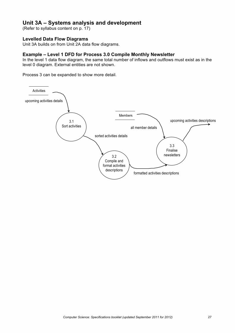
Unit 3A – Systems analysis and development (Refer to syllabus content on p. 17) Levelled Data Flow Diagrams Unit 3A builds on from Unit 2A data flow diagrams. Example – Level 1 DFD for Process 3.0 Compile Monthly Newsletter In the level 1 data flow diagram, the same total number of inflows and outflows must exist as in the level 0 diagram. External entities are not shown. Process 3 can be expanded to show more detail.

3.1 Sort activities

3.3 Finalise

newsletters 3.2 Compile and

format activities descriptions


sorted activities details

formatted activities descriptions

Members

all member details

Activities

upcoming activities descriptions


Managing data Units 1A, 2A and 3A progressively develop knowledge and skills in designing and developing databases. Unit 1A (Refer to syllabus content on p. 9) Components of a single table database—students will identify the fields and data types required to create a single table. Planning for the table structures will not require the use of a diagrammatic tool. Students will apply skills in a single table database application to create a table by defining the fields with their data types and entering records of data into the table. These table records will be manipulated by sorting and searching/querying various fields. Forms will be created to provide a user interface to the data. Simple queries and reports will extract and present data. Unit 2A (Refer to syllabus content on p. 13/14) Unit 2A focuses on spreadsheets and their functions and the design and development of 2 or 3 table relational databases requiring 1:1,1:M, M:1, M:N relationships. Entity Relationship Diagrams will be used to represent these designs. A relational database application will be used to implement:

Tables—define field names; set data types, field formats, default values, primary keys, validation rules and validation text, sort and filter on selected fields Relationships—link tables through primary and foreign keys; enforce referential integrity Queries—create single and multiple table queries; use relational operators (= > >= < <=); use logical operators (and, or, not); use wild cards (*?) Forms—create forms for displaying and entering data Reports—create a report based on a table or a query

Unit 3A (Refer to syllabus content on p. 17) Unit 3A focuses on the conceptual planning of a larger multiple table relational database using normalisation and Entity Relationship Diagrams. Unit 3A builds on the Unit 2A relational database application skills.

Relationships—set cascade inserts, updates and deletes Queries—create parameter, calculated field, concatenated field, aggregation, append, update, delete and queries Visual interface to assist user access


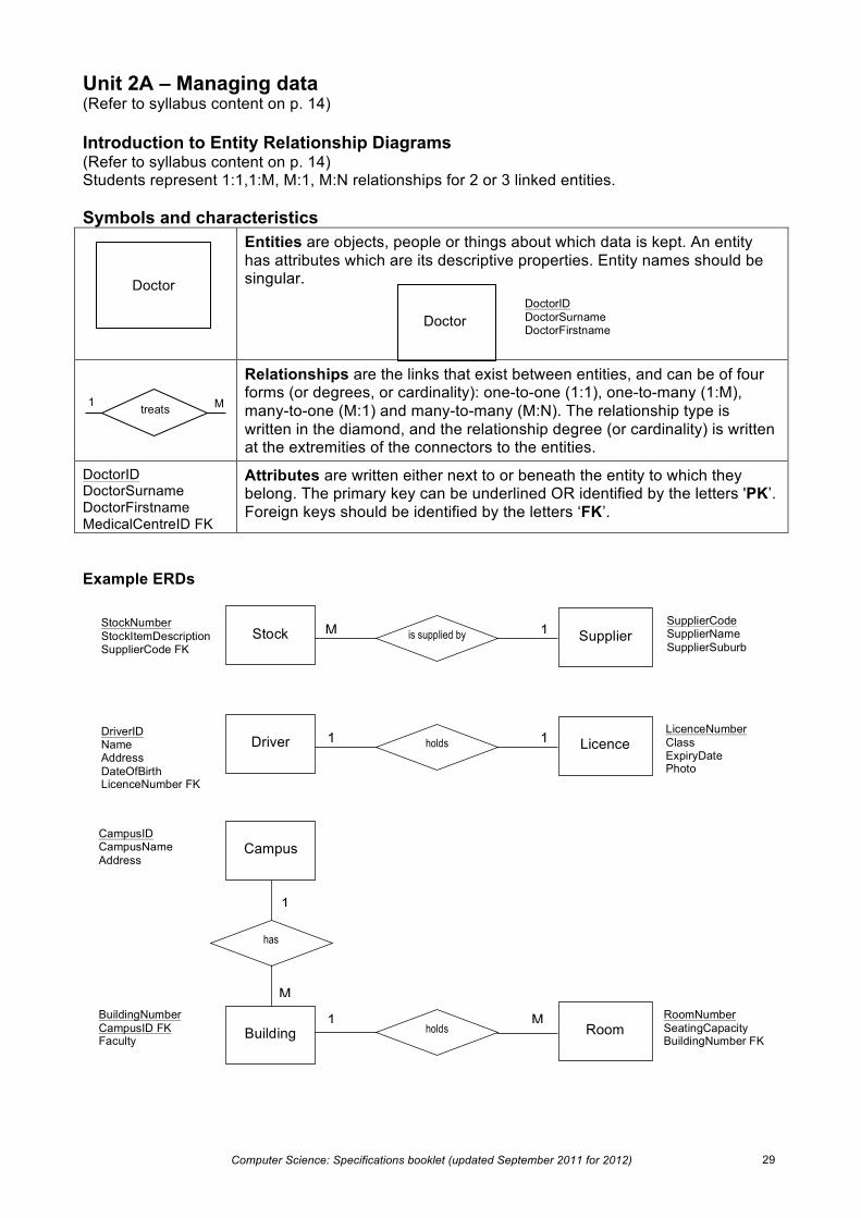
Unit 2A – Managing data (Refer to syllabus content on p. 14) Introduction to Entity Relationship Diagrams (Refer to syllabus content on p. 14) Students represent 1:1,1:M, M:1, M:N relationships for 2 or 3 linked entities. Symbols and characteristics Entities are objects, people or things about which data is kept. An entity

has attributes which are its descriptive properties. Entity names should be singular.

Relationships are the links that exist between entities, and can be of four forms (or degrees, or cardinality): one-to-one (1:1), one-to-many (1:M), many-to-one (M:1) and many-to-many (M:N). The relationship type is written in the diamond, and the relationship degree (or cardinality) is written at the extremities of the connectors to the entities.

DoctorID DoctorSurname DoctorFirstname MedicalCentreID FK

Attributes are written either next to or beneath the entity to which they belong. The primary key can be underlined OR identified by the letters 'PK’. Foreign keys should be identified by the letters ‘FK’.

Example ERDs

Stock Supplier is supplied by 1 M StockNumber StockItemDescription SupplierCode FK

SupplierCode SupplierName SupplierSuburb

Driver Licence holds 1 1 DriverID Name Address DateOfBirth LicenceNumber FK

LicenceNumber Class ExpiryDate Photo

Campus

1 Building holds

M Room

RoomNumber SeatingCapacity BuildingNumber FK

BuildingNumber CampusID FK Faculty

CampusID CampusName Address

has

1

M

M treats 1

Doctor DoctorID DoctorSurname DoctorFirstname

Doctor


The above example shows a composite primary key for the Building entity. This is because the same building number (e.g. 405) may be used on several campuses (e.g. Bentley, Kalgoorlie) so the BuildingNumber and CampusID FK are needed to uniquely identify a building. Unit 3A – Managing data (Refer to syllabus content on p. 18) Keys Primary key A primary key is a single attribute or multiple attributes (composite key) that uniquely identify each tuple in the relation. The primary key attribute must contain unique values. Composite key A composite key is a primary key that is composed of multiple attributes. Foreign key A foreign key is an attribute in a table that stores a value that must match a value in the primary key field in the related table. The foreign key attribute may have duplicate values. Therefore, a foreign key is an attribute in a table that is a primary key in another table. Entity Relationship Diagrams Unit 3A builds on from Unit 2A. Students resolve complex many to many relationships in a multi-table relational database system (three or more entities). Example 1 A pupil has one locker and a locker is used by only one student at a time. The locker details are stored in a separate relation as not all students will have a locker. The following diagram describes this relationship.

Example 2 A pupil can attend many classes and a class is attended by many students. A class is for one course but a course may have many classes. The following diagram describes this relationship.

Pupil Locker has 1 1 LockerID LockerSize Location

StudentID GivenName FamilyName YearGroup LockerID FK

Pupil Class attends N M ClassCode StartDate EndDate CurricCouncilCode FK

StudentID GivenName FamilyName YearGroup ClassCode FK

Course

is for

M

1

CurricCouncilCode CourseName Stage


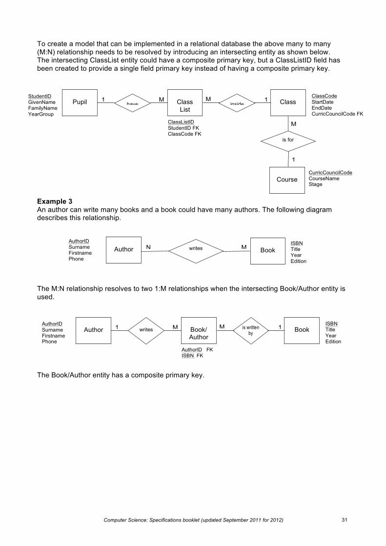
To create a model that can be implemented in a relational database the above many to many (M:N) relationship needs to be resolved by introducing an intersecting entity as shown below. The intersecting ClassList entity could have a composite primary key, but a ClassListID field has been created to provide a single field primary key instead of having a composite primary key.

Example 3 An author can write many books and a book could have many authors. The following diagram describes this relationship.

The M:N relationship resolves to two 1:M relationships when the intersecting Book/Author entity is used.

The Book/Author entity has a composite primary key.

Pupil Class List

Class have inside 1 1 M M StudentID GivenName FamilyName YearGroup

ClassListID StudentID FK ClassCode FK

ClassCode StartDate EndDate CurricCouncilCode FK

Course

is for

M

1

CurricCouncilCode CourseName Stage

Author Book writes M N ISBN Title Year Edition

AuthorID Surname Firstname Phone

Author Book/ Author

Book writes is written by

1 1 M M AuthorID Surname Firstname Phone

AuthorID FK ISBN FK

ISBN Title Year Edition


Unit 3A – Managing data (Refer to syllabus content on p. 18) A data dictionary describes the data that needs to be stored in a database. There are numerous data dictionary formats, but for this course the accepted format for a data dictionary is shown in the example below. The data dictionary is referred to by the staff involved in the creation and maintenance of the database, and any software that interacts with the database. Example—Car table

Element name Data type

Size/ Format Default Description Constraint

CarID Number Unique identifier for each car Required. Automatically created when record added

NumberPlate String 10 Rego number (e.g. 1ACY257) Required ManufacturerID Number The ID of the manufacturer Required Model String 10 The model name (e.g. Falcon) Required BodyType String 10 Sedan Only Sedan, Wagon, Hatchback,

Coupe or Utility should be entered in this field

Required. Limited values allowed

Transmission String 10 Manual Automatic or manual Required NumberOfDoors Number 4 Number of doors including the

hatch if present Note: No cars have more than 7 doors

Required

Colour String 25 Paint colour Required ManufactureDate String 12 Date the car was manufactured

(e.g. 25/10/2007) Required

Airconditioning Boolean True Required SpecialFeatures String 250 Special features such as mag

wheels, mp3 player Optional

SalePrice Number Advertised price for the car Required. Must be greater than zero (> 0)


Unit 3A – Managing Data – Normalisation Normalisation is the process of identifying and eliminating data anomalies and redundancies, thereby improving data integrity and efficiency for storage in a relational database. This process is designed to remove repeated data and improve database design. During normalisation a relation is decomposed (split) into a number of smaller relations suitable for implementation in a relational database. Stage 3 – exam questions will involve defining third normal form (3NF), interpretation of data provided and applying normalisation including:

• identifying reasons why given relations are not in 3NF • identifying and explaining deletion and insertion anomalies as further problems resulting

from repetition • explaining and showing what the relations should look like in 3NF.

What is the starting point? Data needs to be in the form of a relation. This is implemented as a table in a relational database system. A relation has the following characteristics:

• A relation has a name that is distinct from other relation names • There are no repeating groups. • Each cell of the relation contains exactly one atomic (single) value • Each attribute has a distinct name • The values of an attribute are all of the same data type (i.e. can’t mix data types)

The examples below show data about drivers and the cars they may drive. Repeating groups example This data is not a relation because there are repeating groups. A table that contains one or more repeating groups like this is said to be unnormalised.

Driver Licence Number

Driver Firstname

Driver Surname

Driver Email

Car 1 Details

Car 1 Description

Car 2 Details

Car 2 Description

Car 3 Details

Car 3 Description

19289385 John Smith [email protected] 1COB 293, $15000

Blue Corolla

1QAZ 889, $33000

Gold Falcon

1CCT 441, $11000

Green Astra

26453790 Mary Hogg [email protected] 1COB 293, $15000

Blue Corolla

To overcome the problem of repeating groups the table would be reorganised and additional rows added. This is shown in the example below. Multiple values in a cell example This data is not a relation because the Car Details attribute stores multiple values (the car registration and the car value). These values also happen to be different data types.


Driver Firstname

Driver Surname

Driver Email

Car Details

Car Colour

Car Model

Car Manufacturer Website

19289385 John Smith [email protected] 1COB 293, $15000 Blue Corolla www.toyota.com.au 19289385 John Smith [email protected] 1QAZ 889, $33000 Gold Falcon www.ford.com.au 19289385 John Smith [email protected] 1CCT 441, $11000 Green Astra www.holden.com.au 26453790 Mary Hogg [email protected] 1COB 293, $15000 Blue Corolla www.toyota.com.au


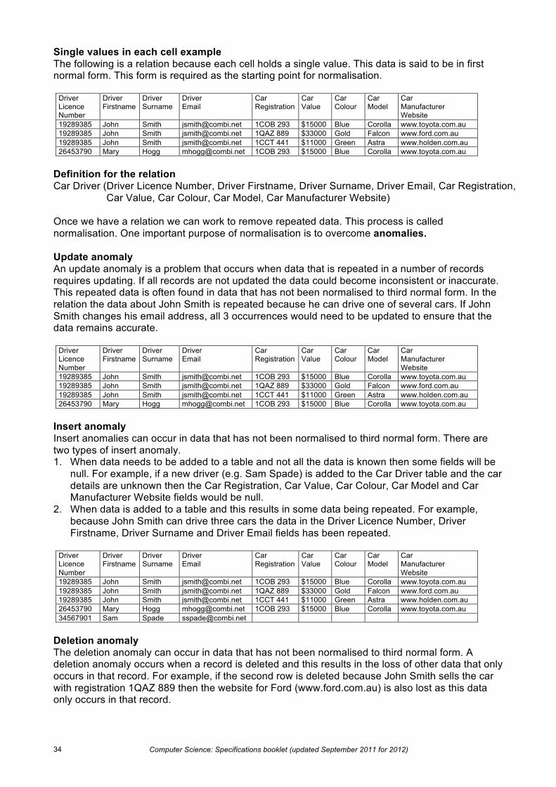
Single values in each cell example The following is a relation because each cell holds a single value. This data is said to be in first normal form. This form is required as the starting point for normalisation.


Driver Firstname

Driver Surname

Driver Email

Car Registration

Car Value

Car Colour

Car Model


19289385 John Smith [email protected] 1COB 293 $15000 Blue Corolla www.toyota.com.au 19289385 John Smith [email protected] 1QAZ 889 $33000 Gold Falcon www.ford.com.au 19289385 John Smith [email protected] 1CCT 441 $11000 Green Astra www.holden.com.au 26453790 Mary Hogg [email protected] 1COB 293 $15000 Blue Corolla www.toyota.com.au

Definition for the relation Car Driver (Driver Licence Number, Driver Firstname, Driver Surname, Driver Email, Car Registration,

Car Value, Car Colour, Car Model, Car Manufacturer Website) Once we have a relation we can work to remove repeated data. This process is called normalisation. One important purpose of normalisation is to overcome anomalies. Update anomaly An update anomaly is a problem that occurs when data that is repeated in a number of records requires updating. If all records are not updated the data could become inconsistent or inaccurate. This repeated data is often found in data that has not been normalised to third normal form. In the relation the data about John Smith is repeated because he can drive one of several cars. If John Smith changes his email address, all 3 occurrences would need to be updated to ensure that the data remains accurate.


Driver Firstname

Driver Surname

Driver Email

Car Registration

Car Value

Car Colour

Car Model


19289385 John Smith [email protected] 1COB 293 $15000 Blue Corolla www.toyota.com.au 19289385 John Smith [email protected] 1QAZ 889 $33000 Gold Falcon www.ford.com.au 19289385 John Smith [email protected] 1CCT 441 $11000 Green Astra www.holden.com.au 26453790 Mary Hogg [email protected] 1COB 293 $15000 Blue Corolla www.toyota.com.au

Insert anomaly Insert anomalies can occur in data that has not been normalised to third normal form. There are two types of insert anomaly. 1. When data needs to be added to a table and not all the data is known then some fields will be

null. For example, if a new driver (e.g. Sam Spade) is added to the Car Driver table and the car details are unknown then the Car Registration, Car Value, Car Colour, Car Model and Car Manufacturer Website fields would be null.

2. When data is added to a table and this results in some data being repeated. For example, because John Smith can drive three cars the data in the Driver Licence Number, Driver Firstname, Driver Surname and Driver Email fields has been repeated.


Driver Firstname

Driver Surname

Driver Email

Car Registration

Car Value

Car Colour

Car Model


19289385 John Smith [email protected] 1COB 293 $15000 Blue Corolla www.toyota.com.au 19289385 John Smith [email protected] 1QAZ 889 $33000 Gold Falcon www.ford.com.au 19289385 John Smith [email protected] 1CCT 441 $11000 Green Astra www.holden.com.au 26453790 Mary Hogg [email protected] 1COB 293 $15000 Blue Corolla www.toyota.com.au 34567901 Sam Spade [email protected]

Deletion anomaly The deletion anomaly can occur in data that has not been normalised to third normal form. A deletion anomaly occurs when a record is deleted and this results in the loss of other data that only occurs in that record. For example, if the second row is deleted because John Smith sells the car with registration 1QAZ 889 then the website for Ford (www.ford.com.au) is also lost as this data only occurs in that record.


Normalisation to Third Normal Form (3NF) (Refer to syllabus content on p. 18) In third normal form (3NF) each non-key attribute is fully functionally dependent on the primary key. Relation not yet in 3NF


Driver Firstname

Driver Surname

Driver Email

Car Registration

Car Value

Car Colour

Car Model

19289385 John Smith [email protected] 1COB 293 $15000 Blue Corolla 19289385 John Smith [email protected] 1QAZ 889 $33000 Gold Falcon 19289385 John Smith [email protected] 1CCT 441 $11000 Green Astra 26453790 Mary Hogg [email protected] 1COB 293 $15000 Blue Corolla

In the above relation the driver’s firstname, surname and email are fully functionally dependent on the driver licence number. However, the car registration (and other car fields) are not. This is because both John Smith and Mary Hogg can both drive the blue Corolla with registration 1COB293. Definition for a relation not yet in 3NF Car Driver (Driver Licence Number, Driver Firstname, Driver Surname, Driver Email, Car Registration, Car Value, Car Colour, Car Model) To normalise data 1. Identify the attributes for each smaller relation. 2. Create each of the smaller relations by moving their attributes into separate relations. For

example move the attributes about the driver to a Driver relation and the attributes about the Car into a Car relation.

3. Create or identify a primary key for each relation. For example Driver Licence Number is unique so it can be identified to be the primary key for the Driver relation, Car Registration is unique in the Car relation, and the combination of Car Registration and Driver Licence Number is unique in the Car Driver relation.

4. Identify or create a link field (foreign key) in the relation that you have removed the attributes from. In the Car Driver relation, the Driver Licence Number will provide a link to the Driver relation and the Car Registration will provide a link to the Car relation.

5. Check that all non-key fields in each relation are fully functionally dependent on the entire primary key.

3NF definitions Driver (Driver Licence Number, Driver Firstname, Driver Surname, Driver Email)

Car (Car Registration, Car Value, Car Colour, Car Model)

Car Driver (Car Registration FK, Driver Licence Number FK)

Note: The above 3NF definitions show the way an exam answer would be expressed. The following relations with sample data are not normally required, but have been provided here so that students can visualise what the definitions represent. 3NF relations Driver Licence Number Driver Firstname Driver Surname Driver Email 19289385 John Smith [email protected] 26453790 Mary Hogg [email protected] Car Registration Car Value Car Colour Car Model Car Registration Driver Licence Number 1COB 293 $15000 Blue Corolla 1COB 293 19289385 1QAZ 889 $33000 Gold Falcon 1QAZ 889 19289385 1CCT 441 $11000 Green Astra 1CCT 441 19289385 1COB 293 26453790


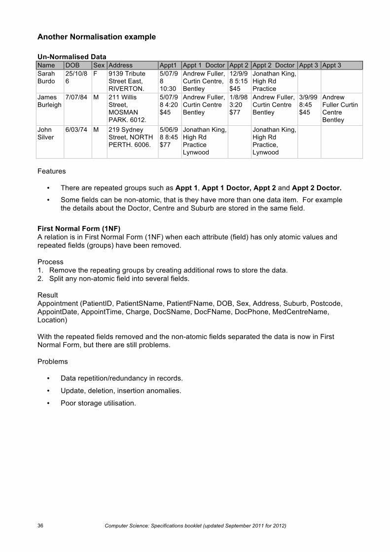
Another Normalisation example Un-Normalised Data Name DOB Sex Address Appt1

Date/Time

Appt 1 Doctor Appt 2 Date/Time

Appt 2 Doctor Appt 3 Date/Time

Appt 3 Doctor Sarah

Burdo 25/10/86

F 9139 Tribute Street East, RIVERTON. 6148.

5/07/98 10:30 $45

Andrew Fuller, Curtin Centre, Bentley

12/9/98 5:15 $45

Jonathan King, High Rd Practice Lynwood

James Burleigh

7/07/84 M 211 Willis Street, MOSMAN PARK. 6012.

5/07/98 4:20 $45

Andrew Fuller, Curtin Centre Bentley

1/8/98 3:20 $77

Andrew Fuller, Curtin Centre Bentley

3/9/99 8:45 $45

Andrew Fuller Curtin Centre Bentley

John Silver

6/03/74 M 219 Sydney Street, NORTH PERTH. 6006.

5/06/98 8:45 $77

Jonathan King, High Rd Practice Lynwood

Jonathan King, High Rd Practice, Lynwood

Features

• There are repeated groups such as Appt 1, Appt 1 Doctor, Appt 2 and Appt 2 Doctor.

• Some fields can be non-atomic, that is they have more than one data item. For example the details about the Doctor, Centre and Suburb are stored in the same field.

First Normal Form (1NF) A relation is in First Normal Form (1NF) when each attribute (field) has only atomic values and repeated fields (groups) have been removed. Process 1. Remove the repeating groups by creating additional rows to store the data. 2. Split any non-atomic field into several fields. Result Appointment (PatientID, PatientSName, PatientFName, DOB, Sex, Address, Suburb, Postcode, AppointDate, AppointTime, Charge, DocSName, DocFName, DocPhone, MedCentreName, Location) With the repeated fields removed and the non-atomic fields separated the data is now in First Normal Form, but there are still problems. Problems

• Data repetition/redundancy in records.

• Update, deletion, insertion anomalies.

• Poor storage utilisation.


To Further Normalise the Data Process 1. Split the existing relation into separate relations by identifying the entity fields and moving them

to a new relation. 2. Create or identify the primary keys for the new relations. 3. Check that the non-key fields in each relation are functionally dependent on the primary key. 4. Leave or create a link field in the relation as the objects are removed. These will become the

foreign keys and will provide the links between the relations. Result Patient (PatientID, PatientSName, PatientFName, DOB, Sex, Address, Suburb, Postcode) Doctor (DoctorID, DocSName, DocFName, DocPhone, MedCentreName, Location) Appointment (PatientID FK, DoctorID FK, AppointDate, AppointTime, Charge) The link fields PatientID FK and DoctorID FK remain in the Appointment relation. These link to the primary key fields in the Patient and Doctor relations. FK is written after each to indicate that it is the foreign key (linking field). Second Normal Form (2NF) A relation is in second normal form (2NF) when each non-key field is functionally dependent on the primary key. Transitive dependencies may still exist in 2NF. Functional Dependency: For each key there will be precisely one matching value in the non-key field. Transitive or partial dependencies still exist in the Doctor relation as the Location of the MedCentre is dependent on the MedCentreName as well as on the DoctorID. That means that the Location is only partially dependent on the key field (DoctorID), and that the dependency on the DoctorID passes through (transitive) the MedCentreName. Some problems still exist in the Doctor table that will cause:

• Data repetition and redundancy

• Update, deletion, insertion anomalies

• Poor storage utilisation.


Third Normal Form (3NF) A set of relations is in third normal form (3NF) when each non-key field is fully functionally dependent on the primary key. Full Functional Dependence: Each non-key field will be functionally dependent only on the key and not on any other field. The Location has a transitive dependency since it is functionally dependent on both DoctorID and MedCentre Name. To achieve full functional dependence, the following decomposition is required. Process Any relation that is still in 2NF is split further to remove transitive dependencies and achieve full functional dependence. Result Patient (PatientID, PatientSName, PatientFName, DOB, Sex, Address, Suburb, Postcode) Doctor (DoctorID, DocSName, DocFName, DocPhone, MedCentreID FK) MedicalCentre (MedCentreID, MedCentreName, Location) Appointment (PatientID FK, DoctorID FK, AppointDate, AppointTime, Charge) The result is a set of relations that can now be implemented in a relational database program.

Documents

COMPUTER SCIENCE - Wikispaces Specifications...Computer Science: Specifications ... Flow chart symbols and pseudocode ... Trace Tables for Desk Checking, Testing and Debugging