Computer Modeling and Simulation of Ultrasonic …file.scirp.org/pdf/MNSMS20110100001_56638573.pdf · Modeling and Numerical Simulation of Material Science, ... In this paper the

Modeling and Numerical Simulation of Material Science, 2011, 1, 1-13 doi:10.4236/mnsms.2011.11001 Published Online October 2011 (http://www.SciRP.org/journal/mnsms)

Copyright © 2011 SciRes. MNSMS

Computer Modeling and Simulation of Ultrasonic System for Material Characterization

Yogendra B. Gandole Department of Electronics, Adarsha Science J.B.Arts and Birla Commerce Mahavidyalaya, Dhamangaon, India

E-mail: [email protected] Received Septenmber 1, 2011; revised October 5, 2011; accepted October 16, 2011

Abstract In this paper the system for simulation, measurement and processing in graphical user interface implementation is presented. The received signal from the simulation is compared to that of an actual measurement in the time domain. The comparison of simulated, experimental data clearly shows that acoustic wave propagation can be modeled. The feasibility has been demonstrated in an ultrasound transducer setup for material property investigations. The results of simulation are compared to experimental measurements. Results obtained fit some much with those found in experiment and show the validity of the used model. The simulation tool therefore provides a way to predict the received signal before anything is built. Furthermore, the use of an ultrasonic simulation package allows for the development of the associated electronics to amplify and process the received ultrasonic signals. Such a virtual design and testing procedure not only can save us time and money, but also provide better understanding on design failures and allow us to modify designs more efficiently and economically. Keywords: Modeling, Simulation, Ultrasonic, Material Characterization, Signal Processing

1. Introduction

Numerical simulations i.e. the use of computers to solve problems by simulating theoretical models is part of new technology that has taken place alongside pure theory and experiment during the last few decades. Numerical simulations permit one to solve problems that may be inaccessible to direct experimental study or too complex for theoretical analysis. Computer simulations can bridge the gap between analysis and experiment. Numerical simulations analysis and experiment cover mutual weak- ness of both experiment and theory. These simulations will remain a third dimension in ultrasonic measurements, of equal status and importance to experiment and analy-sis. It has taken a permanent place in all aspects of ultra-sonic measurements from basic research to engineering design. The computer experiment is a new and poten-tially powerful tool. By combining conventional theory, experiment and computer simulation, one can discover new and unsolved aspects of natural process. These as-pects could often neither have been understood nor rev-eled by analysis or experiments alone.

There might be many use of ultrasound but a common one is its application to non-destructive evaluation. Pulsed

ultrasonic is finding an increasing number of applications in research and industrial nondestructive testing. In such evaluation, one tries to obtain information about the inner parts of an ensemble without dismantling it. In an ultrasonic system, a transducer consists of a collection of material layers. The design and optimization of a multi- layered transducer is a complicated engineering task that involves knowledge of physical acoustics, analog electronics, and the acoustical properties of the materials involved. This task is made even more difficult by the lack of available information about frequency and thermal dependencies of these materials characteristics. The optimal combination of suitable materials can be found by trial and error, but not without considerable time and cost, both of which can be minimized through the use of simulations. The aim of this paper is to present a tool which provides a simulation of the received signal prior to construction. Of the different ways to model the electro-acoustic system, a total electrical simulation tool is used for the following reasons. First, the modeling of acoustic wave propagation in one dimension by electrical lines can be handled with a certain ease; second the associated electronics used to excite, receive, amplify and process the signals can be designed to meet the application’s

Y. B. GANDOLE 2

specifications prior to building system. This paper pre- sents a simulation solution to ease the selection process. The electronic software simulation package used is PSPICE [15]. The use of PSPICE provides an opportu- nity to simulate the complex set of excitation electronics, the ultrasonic transducer, the material under investigation, and the receiving electronics. Electrical analogies of one- dimensional acoustic phenomenons have studied over the years. Mason (1942) [23], modeled electromechanical transducers with a lumped equivalent circuit. Redwood (1961) [11], incorporated a transmission line into Ma- son’s model to obtain useful information about the transient response of a piezoelectric transducer. With the transmission line, one can represent the time delay necessary for a mechanical signal to travel from one side of the transducer to the other. In the case of a plate transducer, the derivation of both models includes a negative capacitor. Using SPICE and an equivalent circuit appro- ximating the negative capacitor, Morris and Hutchens (1986) [17], simulated Redwood’s implementtation of Mason’s model. Krimholtz et al. (1970) [16], presented another equivalent circuit for elementary piezoelectric transducer. Leach (1994) [22], used controlled current and voltage sources instead of transformers. Leach mathe- matically derives his model by adding terms equal to zero in one of the devices electromechanical equations to obtain the form of the telegraphist’s equation. Puttmer et al. (1996) [3], used a lossy transmission line in Leach’s model to account for acoustical attenuation. Benny et al. (2000) [4], outlines a method that has been implemented to predict and measure the acoustic radiation generated by ultrasonic transducers operating into air in continuous wave mode. A comparison of experimental and simulated results for piezoelectric composite, piezoelectric po- lymer, and electrostatic transducers is then presented to demonstrate some quite different airborne ultrasonic beam-profile characteristics. San Emeterio et al. ( 2004) [19], present an approximate frequency domain electro-acoustic model for pulsed piezoelectric ultrasonic transmitters which by, integrating partial models of the different stages, allows the computation of the emission transfer function and output force temporal waveform. Hirsekon et al. (2004) [13], perform numerical simulations of acoustic wave propagation through sonic crystals consisting of local resonators using the local interaction simulation approach (LISA). The current work applies the approach of Puttmer et al. [3] to liquids and piezoelectric transducer to obtain an electrical analogue of one-dimensional, acoustic wave propagation through such materials. In order to keep things at a manageable level, the following simplifications and assumptions are made. The acoustic propagation travels along one direction and consist of planner longitudinal waves, which are normal to the direction of propagation. The amplitudes are small

enough to keep things in linear regions of the devices such that the principle of superposition is not violated. From available material data, such as the modulus of elas- ticity and Poisson’s ratio, the necessary electrical parameters are deduced. Validation of the theory is achieved by comparing experimental data obtained from different liquids at fixed frequency and temperature.

2. Modeling

The piezoelectric phenomenon is modeled using con-trolled voltage and current sources [22] (Figure 1).

The equivalent circuit consists of the static capacitance C0 (capacitance between the electrodes), a transmission line (representing the mechanical part of the piezoelectric transducer) and two controlled sources for coupling between the electrical and mechanical part of the circuit. Suppose a ultrasonic pulse travels through a medium with a finite speed c (m/s). This pulse can be pictured as a disturbance to which the medium reacts to. In the case of longitudinal wave, the disturbance is a compression or rarefaction of matter, which the medium displaces to return to its equilibrium state. The compression and rarefaction within the medium is related to its density ρ (kg/m3), and the restoring force is related to the medium’s bulk modulus M (pa) [10]. Their relationship to the speed of sound is:

c vM

Similarly, in an electrical transmission line an electrical pulse can travel through it. These pulses are received at the other end of the line after a very short but finite time. The pulses travel at a certain velocity. Similar to the acoustic wave, the electrical pulses are concentrations and rarefaction of electrons within the transmission line [8].

A distributed-parameter network with the circuit parameters distributed throughout the line can approximate a lossy transmission line. One line segment with the length

Figure 1. Equivalent circuit for piezoelectric transducer (the leach model). Here l is the thickness, f is the force, u is the particle velocity, v is the electrical voltage, i is the elec-trical current, h is the piezoelectric constant and s is the Laplace operator.


3Y. B. GANDOLE

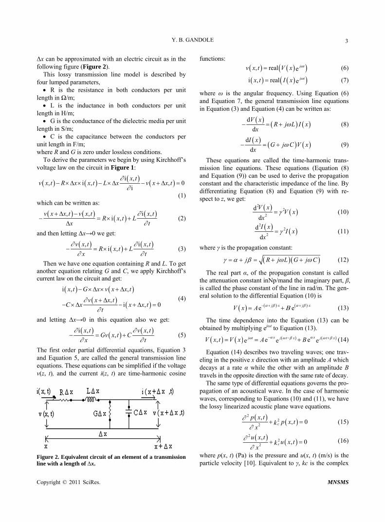
Δx can be approximated with an electric circuit as in the following figure (Figure 2).

This lossy transmission line model is described by four lumped parameters, R is the resistance in both conductors per unit

length in Ω/m; L is the inductance in both conductors per unit

length in H/m; G is the conductance of the dielectric media per unit

length in S/m; C is the capacitance between the conductors per

unit length in F/m; where R and G is zero under lossless conditions.

To derive the parameters we begin by using Kirchhoff’s voltage law on the circuit in Figure 1:

i ,, i , ,

i

x tv x t R x x t L x v x x t

0

(1) which can be written as:

, , ii ,

v x x t v x t x tR x t L

,

x t

(2)

and then letting Δx→0 we get:

, ii ,

v x t x tR x t L

,

x t

(3)

Then we have one equation containing R and L. To get another equation relating G and C, we apply Kirchhoff’s current law on the circuit and get:

i , ,

,i ,

x t G x v x x t

v x x tC x x x t

t

0

(4)

and letting Δx→0 in this equation also we get:

i , ,,

x tGv x t C

v x t

x t

(5)

The first order partial differential equations, Equation 3 and Equation 5, are called the general transmission line equations. These equations can be simplified if the voltage v(z, t), and the current i(z, t) are time-harmonic cosine

Figure 2. Equivalent circuit of an element of a transmission line with a length of Δx.

functions:

, real e j tv x t V x (6)

i , real e j tx t I x (7)

where ω is the angular frequency. Using Equation (6) and Equation 7, the general transmission line equations in Equation (3) and Equation (4) can be written as:

d

d

V xR j L I x

x (8)

d

d

I xG j C V x

x (9)

These equations are called the time-harmonic transmission line equations. These equations (Equation (8) and Equation (9)) can be used to derive the propagation constant and the characteristic impedance of the line. By differentiating Equation (8) and Equation (9) with re-spect to z, we get:

2

2

2

d

d

V xV x

x (10)

2

2

2

d

d

I xI x

x (11)

where γ is the propagation constant:

j R j L G j C (12)

The real part α, of the propagation constant is called the attenuation constant inNp/mand the imaginary part, β, is called the phase constant of the line in rad/m. The gen-eral solution to the differential Equation (10) is

e ej x jV x A x (13)

The time dependence into the Equation (13) can be obtained by multiplying ejωt to Equation (13).

, e ee e ex x j t j t x jV x t V x A B t x (14)

Equation (14) describes two traveling waves; one traveling in the positive x direction with an amplitude A which decays at a rate α while the other with an amplitude B travels in the opposite direction with the same rate of decay.

The same type of differential equations governs the propagation of an acoustical wave. In the case of harmonic waves, corresponding to Equations (10) and (11), we have the lossy linearized acoustic plane wave equations.

2

22

,,c

p x tp x tk

x

0 (15)

2

22

,,c

u x tu x tk

x

0 (16)

where p(x, t) (Pa) is the pressure and u(x, t) (m/s) is the particle velocity [10]. Equivalent to γ, kc is the complex


Y. B. GANDOLE 4

wave number composed of an attenuation constant a (Np/m) and a wave number k (rad/m). The general solution of the wave Equation (15) is

, e e e ex j k x x j k xp x t A B (17)

and is identical to the solutions obtained in transmission line’s represented by Equation (14) . Equation (16) has a solution of the same form. The complex wave number kc is given as

1

1ck

c j t

(18)

1

22

2

1 11

2 1c

(19)

1

22

2

1 11

2 1ck

c

(20)

In order to unify the two theories, an impedance type analogy is chosen where mechanical force is represented by voltage and current represents particle velocity. The characteristic impedance becomes important at the boundaries because there the continuity conditions have to be satisfied. Pressure and normal particle velocity must be continuous at the boundaries as voltage and current must be continuous at connections. For the lossy transmission line [8], the characteristic impedance Zel is:

e1R j L

ZG j C

(21)

and for the lossy acoustic medium[10] ,the characteristic acoustic impedance Z a is:

1Z a pc j (22)

where ρ is the density of the medium. Expanding Equation (21) and Equation (12), we obtain,

11

2e1

L RZ

C j L C

G (23)

and 1

2

R GLC j LC

L C

(24)

Considering small but non-negligible losses where R ωL, G ωC and ωτ 1. the second term of Equa-

tion (23) is negligible, leaving the characteristic imped-

ance as

L C Similarly from Equation (22), the low

loss acoustical characteristic impedance can be approximated as ρc. Also, the wave number k from Equation (20) become ω/c. To correlate the two characteristic impedances, we choose an impedance type analogy (Figure 1),

in which the force, (and not pressure) is represented by voltage and the particle velocity is represented by current. The equivalence between the two systems is

e1 ZaAZ (25)

where A(m2) is the cross-sectional area of the acoustic beam.

Assisted with the definition of the low loss characteristic impedances equation, following relationships can be obtained

L A (26)

The real part of Equation (24) is the attenuation con-stant

2

1C

A c

(27)

1 1

2 2

RLC LC

L C

G

c

(28)

Drawing a parallel with the classical theory of acoustic attenuation,

classical v t

where αv is the coefficient of attenuation due to viscous losses, and αtc is the coefficient of attenuation due to thermal conduction. From Equations (26)-(28), we can solve for R and G to model the attenuations such that,

2 VR cA (29)

2 tcG

cA

(30)

Because the material layers used in this paper have a low heat conductance, the loss due to thermal conduction is negligible, and we let the conductance G = 0.

Equations (26), (27) and (29) are the final equations required for simulation purpose.

2.1. Piezoelectric Transducer

An important task when designing ultrasonic transducers and complete transducer system is the simulation of possible configuration prior to construction. Ultrasonic transducer usually consists of a piezoelectric element and non-piezoelectric layers for encapsulation and acoustic matching. Points of interest are effects of backing materials, matching layers, piezoelectric materials, layer thickness, electrical matching and coupling on transducer characteristics like bandwidth, time response on different excitation signals and ring down behavior. As presented in the introduction, different models have been devel- oped over the years to simulate these transducers. Me- chanically, a transmiszength is selected to achieve the desired center frequency f(Hz) of the transducer. With fixed ends, the piezoelectric plate has a fundamental re-


5Y. B. GANDOLE

sonant frequency as:

2

c Tf

len (31)

where c(T) is the velocity of sound through it at temperature T.

Using Equations (26)-(27) and the piezoceramic’s density ρ, required for transmission line, L and C values can be calculated. The mechanical factor Qm describes the shape of the resonance peak in the frequency domain. The relation between angular frequency ω, inductance L and the resistance R is given as [3]:

LQm T

R

(32)

In the electrical section, the static capacitance Co is calculated as:

s T ACo T

len (33)

where εs (C2/N·m2) is the permittivity with constant strain [9].

The latter is related to the permittivity with constant stress (free) εT as

T

s 2

1

1 k

T

TT

(34)

Where k(T) is the piezoelectric coupling constant. The mechanical and electrical sections interact with

two current controlled sources. From the mechanical side, the deformation itself is not measurable, but the current representing the rate of deformation is the difference between the velocity of each surface normal to the propagation path, represented by the currents u1 and u2, is the rate of deformation. This current (u1 - u2) controls the current source F1. It has a gain equal to the product of the transmitting constant h(N/C), and the capacitance C0. h is the ratio of the piezoelectric stress constant e33 (C/m2) in the direction of propagation and the permittivity with zero or constant strain εS. In the thickness mode it is [9]

33es

Th T

T (35)

This source’s output is in parallel with the capacitor Co. The result is a potential difference across the capacitor that is proportional to the deformation. In the electrical section, the current through the capacitor Co controls the current source F2. The gain for this second current source is h. Its output needs to be integrated to obtain the total charge on the electrodes that proportionally deforms the transducer. The integration is performed by the capacitor C1. The voltage controlled voltage source E1 with unity gain is a one-way isolation for the integrator.

2.2. Liquids

The speed of sound in a liquid is given as:

c S TKT

T

where Ks is the adiabatic bulk modulus [2]. Starting with the Navier-Stokes equation, Kinsler et al.

[10] derive the following formula for the coefficient of attenuation due to viscosity

2

3

2

3T T

T Tc

where η(T) is the viscosity of liquid. One of the assumptions made in this derivation is that the bulk viscosity is negligible. Parameters that are temperature sensitive, like viscosity, need to be obtained at the desired temperature for single temperature simulation or as a function of temperature for parametric simulation over a temperature range.

3. Experimental Setup

The block diagram of Pulser-Receiver system is shown in Figure 3. The experimental circuit is designed by Gandole et al. [18] is used in this set up. The RF pulse generator generates sharp radio frequency pulses of va- rious frequencies in the range 1 MHz to 10 MHz, having pulse width 2 to 60 microseconds. The repetition rate of the pulses is 1 KHz. The radio frequency pulse is fed to the ultrasonic transducer (piezoelectric). The transducer excited and sends ultrasonic pulse through the sample. The receiver transducer, which is at the other end of the sample, converts the received ultrasonic pulse into an electrical signal (RF pulse). The details of pulser circuit are given in Yawale et al. [18]. This RF pulse is fed to an amplifier consists of single stage which is assembled by using transistor BF195. The output of single stage amplifier is again amplified with the help of another amplifier using IC CA3028 in cascade mode. The overall characteristics of amplifier are as: gain = 50 dB; bandwidth = 15 MHz; input impedance = 10.5 kΩ and low noise. The stability of IC 3028 amplifier is much higher because of small reverse feedback [12]. After the detection of signal through LM 393 (wide band zero cross detector), the detected signal is fed to unity gain buffer, designed using high speed, low power Op-amp AD 826. The character-istics of AD826 are 50 MHz unity gain bandwidth, 350 V/μs slew rate, 70 ns settling time to 0.01% and 2.0 mV max input offset voltage. This detected signal is then given to reset input of RS flip-flop, while the output of IC 74121 of RF pulse generator is used to set the flip-flop. Therefore a single pulse is obtained at the output,


Y. B. GANDOLE


6

Figure 3. Block diagram of experimental setup. whose width is the time taken by the pulse to travel through the sample. Time meter having accuracy of 0.01 μs measures the width of the pulse. For the measurement of velocity and attenuation, the sender transducer is firmly fixed at one end of the measuring cell (Figure 4), while receiving transducer is fixed to movable scale (Griffin and Tatlock Ltd. London, Make) having least count 0.0001 cm. The system communicates with per-sonal computer (PC) through 12-bit DAS card. For communication, control and set of parameters of ultra-sonic system Graphical user interface (GUI) were created (Figure 5). GUI provides general data represent- tation. In GUI it is possible to change almost all of parameters of measured signal and parameters of signal processing. For link-up with system functions for control drivers in Dynalog system were used. Then parameters for com-munication with system were set up. In windows (Figure 5), it is possible to select channel number, polar- ity (unipolar/Bipolar) and Range using DAQ configure- tion frame. “RUN DAQ” frame is used to open the card using “open” command button, close the card using “close” command button. “Start Scan” command button samples the data (voltage level and time) and stores in buffer memory. “Stop Scan” command button stop the sampling process. Measurement and analysis of received ultrasonic signal is achieved by “Measurement and Analysis” frame. The command button “Transient Response” opens the new window, which displays the transient response of the sampled data. Using the cursor point it is possible to measure the time and pulse height of received signal. This data is stored in database for further analysis.

Figure 4. Probe layout for liquid samples.

Figure 5. GUI screen of experimental ultrasonic system.

The liquid sample was contained in a measurement

cell as shown in Figure 3. A glass bottle of suitable size was cut to form a measuring cell. The bottle was fixed with adhesive araldite in an inner space of double walled chamber which was made up of thick galvanized sheet. Water circulation arrangement was made through ther- mostat. Dimensions of double walled chamber are as: height of doubled walled chamber 6.5 inches, outer diameter 5.5 inches, inner diameter 3.25 inches, height of glass bottle 7.5 inches. The double walled chamber was provided with inlet and outlet for constant temperature

Matched pair of quartz transducers completely sealed (supplied by electrosonic industries, New Delhi) was used for ultrasonic generation and detection. The frequency of measurement was 2 MHz. Diameter of transducer was 25.4 mm. Also the second set of matched pair of transducer PZT-5A (supplied by Panametrics Videoscan V3456) with center frequency 5 MHz was used. Diame- ter of transducer was 12.5 mm.

7Y. B. GANDOLE

water circulation. The lower surface of cell (glass bottle) and double walled chamber were in the same plane. The double walled chamber was kept on disc to which sender transducer was fixed. Applying silicone grease made the contact of sender transducer and measuring cell. The lower surface of measuring cell acted as acoustic window through which ultrasonic waves could enter in the measuring cell. The clamps ware provided between double walled chamber and disc to avoid movement of doubled walled chamber and hence of measuring cell during the ultrasonic measurements.

4. Simulation Setup

The analogous circuit setup is described in Figure 6. Si- mulation code is given below, to describe the circuit.

4.1. The Pulser-Receiver

The pulser circuitry, shown in Figure 6 consists of a pulse generator using pulse source (V2) having 5 V pulsed voltage, 0 sec delay, 1ns rise and fall time, 2us pulse width and 1ms period. Another source (V3) is sinusoidal source having 0 offset voltage, 5V peak voltage, 0 sec delay, 5MHz frequency, 0 damping factor and phase

delay followed by TTL7400, 7407, 1KΩ resistor (R3), 20V dc supply (V1) and 2nf capacitor (C3). The pulse start at 20 V and decays to 0 V in 2us. The output of the capacitor is connected to the electrical part of the transducer and a parallel damping resistor (R4). The receiving and amplifying electronics is not implemented in this schematic.

4.2. The Transducer and Liquid Samples

The matched pair of piezoelectric material PZT-5A, whose material data is obtained from Berlincourt [4], was chosen and given in Table 1. For simplicity, the front wear plate is omitted, and to reduce the ringing of the echoes a backing material is selected with a characteristic acoustic impedance of 15.8 MPas/m. The thickness of the backing layer should be selected such that no echoes return from it. This facts permits us to model the backing layer with a resistor (R2 = R6 = 2KΩ). Another matched pair of quartz transducers supplied by electro sonic industries, New Delhi, was chosen and whose material data is given in Table 1. The data obtained for the lower surface of cell (glass bottle) is given in Table 1. The data in Table 1, for liquid samples was obtained from standard references [6,24,25].

Figure 6. Simulation circuit of the experimental setup; Here Static capacitance (Co) = C1 = C4, R1 = R5, F1 = F3, F2 = F4, E1 = E2.

Table 1. Physical properties of materials at 25˚C.

S. No. Physical Properties at 25˚C PZT-5 A Quartz Transducer

1 Density (ρ) Kg/m3 7750 6820

2 Mechanical Q (Qm) 75 2 × 106

3 Sound velocity (m/s) 4350 5660

4 Permitivity with constant strain (εS) [C2/N·m2] 7.35 × 10–9 4.03 × 10–11

5 Piezoelectric stress constant (e33) [C/m2] 15.8 0.171


Y. B. GANDOLE 8

4.3. Graphical User Interface for Simulation

Analysis

Figure 7 shows the Graphical User Interface (“UT Meas- urements”) for easy access to the basic functionality of the modeled ultrasonic system using PSPICEA_D. The results of mixed-signal simulations can then be plotted in the same Probe window with little effort. The newly de- veloped Graphical User Interface heightens the level of clarity, accelerates the speed of navigation and improves control of information flow enabling end users to take advantage of the systems full potential.

5. Signal Processing

5.1. Time Domain

Comparing the received signals from experiments and simulations in the time domain. The simulation signal is shown in (a) and the measured signal is shown in (b). Figure 8 shows the first 30 us pulse received by the 5 MHz transducer with an ethanol sample at 25˚C.

Figure 9 shows the first 32 us pulse received by the 5

MHz transducer in Methanol at 25˚C. Figure 10 shows the first 36 us pulse received by the 5

MHz transducer in Carbon tetra chloride at 25˚C. Figure 11 shows the first 30 us pulse received by the 5

MHz transducer in Acetone at 25˚C. Figure 12 shows the first 27 us pulse received by the 5

MHz transducer in benzene at 25˚C. Figure 13 shows the first 25 us pulse received by the 5

MHz transducer with a distilled water sample at 25˚C. The Table 6 shows the comparison between the lit-

erature values and simulation values of ultrasonic velocity and attenuation for the liquid samples.

Figures 14(a)-(e) show the first 50 us pulse received by the 2 MHz crystal transducer with binary liquid mixtures of Methanol and benzene sample at 25˚C.

Figures 15(a)-(e) show the first 50 us pulse received by the 2 MHz crystal transducer with binary liquid mixtures of Methanol and benzene sample at 25˚C.

The Tables 7(a)-(b) show the comparison between the Experimental values and simulation values of ultrasonic velocity and attenuation for the binary liquid mixture samples.

Figure 7. GUI Screen for modeling and simulation of ultrasonic system.

(a) (b)

Figure 8. Complete transient received by 5 MHz transducer with an ethanol sample at 25˚C.


9Y. B. GANDOLE

(a) (b)

Figure 9. Complete transient received by the 5 MHz transducer at 25˚C, in Methanol.

(a) (b)

Figure 10. Complete transient received by 5 MHz transducer at 25˚C, in Carbon tetra chloride.

(a) (b)

Figure 11. Complete transient received by 5 MHz transducer at 25˚C in Acetone.

(a) (b)

Figure 12. Complete transient received by 5 MHz transducer at 25˚C, in benzene.

(a) (b)

Figure 13. Complete transient received by 5 MHz transducer at 25˚C, in distilled water.


Y. B. GANDOLE


10

Methanol (X1) + Benzene (X2) Methanol (X1) + Acetone (X2)

(a) (a)

Figure 14(a). Methanol + Benzene Mole fraction X1 = 0.1952.

Figure 15(a). Methanol + Acetone Mole fraction X1 = 0.1678.

(b) (b)

Figure 15(b). Methanol + Acetone Mole fraction X1 = 0.4375.

Figure 14(b). Methanol + Benzene Mole fraction X1 = 0.4834.

(c) (c)

Figure 15(c). Methanol + Acetone Mole fraction X1 = 0.6447.

Figure 14(c). Methanol + Benzene Mole fraction X1 = 0.6858.

(d) (d)

Figure 15(d). Methanol + Acetone Mole fraction X1 = 0.8090.

Figure 14(d). Methanol + Benzene Mole fraction X1 = 0.8359.

(e) (e)

Figure 14(e). Methanol + Benzene Mole fraction X1 = 0.9516.

Figure 15(e). Methanol + Acetone Mole fraction X1 = 0.8090.

11Y. B. GANDOLE

Table 6. Ultrasonic velocity and attenuation at 25˚C for 5 MHz frequency.

S. No. Sample (Liquid) Velocity (m/s) Attenuation (x/f2) 10–15s2/m

Measured by simulation Literature value Measured by simulation Literature value

1 Ethanol 1207.2431 1207 [25] 48.3151 48.5 [25]

2 Methanol 1103.3468 1103 [25] 31.9376 30.2 [25], [6]

3 Carbon tetrachloride 930.5210 930 [25] 538.8767 538 [25], 545 [1]

4 Acetone 1174.6280 1174 [24] 53.6800 54 [24], 30 [7]

5 Benzene 1310.0426 1310 [25] 837.2724 873 [25]

6 Distilled water 1497.0059 1497[25] 21.9782 22 [25]

Table 7. (a) Comparison of measured and simulated values of ultrasonic velocities and attenuations in binary liquid mixtures (Methanol and Benzene) at 25˚C; (b) Comparison of measured and simulated values of ultrasonic velocities and attenuations in binary liquid mixtures ( Methanol and Acetone) at 25˚C.

(a)

Measured Simulated Binary liquid mixture Mole fraction of X1

Velocity (m/s) α (dB/m) Velocity (m/s) α (dB/m)

0.1952 1196.015 29.224 1196.289 28.877

0.4834 1135.165 20.279 1135.426 20.038

0.6858 1124.155 15.185 1124.409 15.004

0.8359 1110.130 11.305 1110.378 11.171

Methanol (X1)

+ Benzene

(X2) 0.9516 1066.865 9.555 1067.105 9.441

1) Statistical analysis

a) Greatest percentage deviation of simulated velocity from experimental value 0.022%

Greatest percentage deviation of simulated attenuation from experimental value 1.20%

Calculated chi-squared value (velocity) 0.0002

Calculated chi-squared value (attenuation) 0.0122

Critical values of chi-square at 0.05 level (degree of freedom = 4) 9.488

(b)

Measured Simulated Binary liquid mixture Mole fraction of X1

Velocity (m/s) α (dB/m) Velocity (m/s) α (dB/m)

0.1678 1095.125 29.245 1095.375 28.896

0.4375 1094.735 23.455 1094.985 23.175

0.6447 1087.045 19.952 1087.287 19.715

0.8090 1069.845 14.725 1069.608 14.549

Methanol (X1)

+ Acetone

(X2) 0.9423 1057.055 13.225 1057.291 13.067

1) Statistical analysis

a) Greatest percentage deviation of simulated velocity from experimental value 0.022%

Greatest percentage deviation of simulated attenuation from experimental value 1.20%

Calculated chi-squared value (velocity) 0.0002

Calculated chi-squared value (attenuation) 0.0144

Critical values of chi-square at 0.05 level (degree of freedom = 4) 9.488


Y. B. GANDOLE 12

6. Conclusions

Analogy between acoustic media and transmission lines is reviewed and an analogous electrical model of an ultrasonic transducer using controlled sources is discussed. A Simulation model of a complete ultrasonic system is presented. The received signal from the simulation is compared to that of an actual measurement in the time domain. The comparison of simulated, experimental data clearly shows that temperature and frequency dependencies of parameters of relevance to acoustic wave propagation can be modeled. The feasibility has been demonstrated in an ultrasound transducer setup for material property investigations. Comparisons were made for attenuation and velocity of sound for ethanol, methanol, carbon tetrachloride, acetone, benzene and distilled water. For these materials, the agreement is good. The simulation tool therefore provides a way to predict the received signal before anything is built. Furthermore, the use of an ultrasonic simulation package allows for the development of the associated electronics to amplify and process the received ultrasonic signals.

7. References

[1] A. A. Berdyev and B. Khemraev, Russian Journal of Physical Chemistry, Vol. 41, 1976, p. 1490.

[2] A. D. Pierce, “An Introduction to Its Physic Principles and Applications,” Woodburg, New York, 1989.

[3] A. Puttmer, P. Hauptmann, R. Lucklum, O. Krause and B. Henning, “SPICE Model for Lossy Piezoceramic Trans-ducers,” IEEE Transactions on Ultrasonics, Ferroelec-trics and Frequency Control, Vol. 44, No. 1, 1997, pp. 60-66. doi:10.1109/58.585191

[4] G. Benny, G. Hayward and R. Chapman, “Beam Profile Measurements and Simulations for Ultrasonic Transduc-ers Operating in Air,” Journal of the Acoustical Society of America, Vol. 107, No. 4, 2000, pp. 2089-2100. doi:10.1121/1.428491

[5] D. Berlincourt, H. A. Krueger and C. Near, “Important Properties of Morgan Electroceramics,” Morgan Electro-ceramics, Technical Publication, TP-226, 2001.

[6] D. E. Gray, “American Institute of Physics Handbook,” 3rd Edition, Mc Graw-Hill, New York, 1972.

[7] D. F. Evans, J. Thomas, J. A. Nadas and M. A. Matesich, Journal of Physics and Chemistry, Vol. 75, No. 11, 1971, pp. 1714-1722. doi:10.1021/j100906a013

[8] D. K. Cheng, “Field and Wave Electromagnetics,” 2nd Edition, Addison-Wesley, Reading, 1989.

[9] G. S. Kino, “Acoustic Waves: Devices, Imaging and Analog Signal Processing,” Prentice-Hall, Englewood Cliffs, 1988.

[10] L. E. Kinsler, A. R. Frey, A. B. Coppens and J. V. Sand-ers, “Fundamentals of Acoustics,” 3rd Edition, Wiley,

New York, 1982.

[11] M. Redwood, “Transient Performance of a Piezoelectric- transducer,” Journal of the Acoustical Society of America, Vol. 33, 1961, pp. 527-536. doi:10.1121/1.1908709

[12] M. G. S. Ali, “Analysis of Broadband Piezoelectric Transducers by Discreet Time Model,” Egyptian Journal of Solids, Vol. 23, 2000, pp. 287-295.

[13] M. Hirsekorn, P. P. Delsanto, N. K. Batra and P. Matic, “Modellling and Simulation of Acoustic Wave Propagation in Locally Resonant Sonic Materials,” Ultrasonics, Vol. 42, No. 1-9, 2004, pp. 231-235. doi:10.1016/j.ultras.2004.01.014

[14] J. Millman and C. Halkias, “Integrated Electronics,” McHill Ltd., Tokyo, 1972, p. 560.

[15] M. H. Rashid, “SPICE for Circuits and Electronics Using PSPICE,” 2nd Edition, Printice Hall of India Pvt, Ltd., New Delhi, 2002.

[16] R. Krimholtz, D. A. Leedom and G. L. Matthei, “New Equivalent Circuits for Elementary Piezoelectric Trans-ducers,” Electronics Letters, Vol. 6, 1970, pp. 398-399. doi:10.1049/el:19700280

[17] S. A. Morris and C. G. Hutchens, “Implementation of Mason’s Model on Circuit Analysis Programs,” IEEE Transactions on Ultrasonics, Ferroelectrics and Fre-quency Control, Vol. 33, 1986, pp. 295-298.

[18] Y. B. Gandole, S. P. Yawale and S. S. Yawale, “Simpli-fied Instrumentation for Ultrasonic Measurements,” Elec-tronic Technical Acoustics, Vol. 35, 2005.

[19] J. L. San Emeterio, A. Ramos, P. T. sanz, A. Ruiz and A. Azbaid, “Modeling NDT Piezoelectric Ultrasonic Trans-mitter,” Ultrasonics, Vol. 42, No. 1-9, 2004, pp. 277-281. doi:10.1016/j.ultras.2004.01.021

[20] J. P. Sferruzza, F. Chavrier, A. Birer and D. Cathignol, “Numerical Simulation of the Electro-Acoustical Re-sponse of a Transducer Excited by a Time-Varying Elec-trical Circuit,” IEEE Transactions on Ultrasonics, Ferro-electrics and Frequency Control, Vol. 49, No. 2, 2002, pp. 177-183.

[21] S. H. Lee, “Shear Viscosity of Benzene, Toluene, and p-Xylene by Non-Equilibrium Molecular Dynamics Simulations,” Bulletin of the Korean Chemical Society, Vol. 25, No. 2, 2004, pp. 321-324. doi:10.5012/bkcs.2004.25.2.321

[22] W. M. Leach, “Controlled-Source Analogous Circuits and SPICE Models for Piezoelectric Transducers,” IEEE Transactions on Ultrasonics, Ferroelectrics and Fre-quency Control, Vol. 41, 1994, pp. 60-66.

[23] W. P. Mason, “Electromechanical Transducers and Wave Filters,” Van Nostrand, New York, 1942.

[24] W. Schaaff, “Numerical Data and Functional Relational-ships in Science and Technology,” In: K. H. Hellwege and A. M. Hellweg, Eds., New Seris Group II: Atomic and Molecular Physics, Vol. 5: Molecular Acoustics, Springer-Verlag, Berlin, 1967.

[25] Weast, C. Robert, “Handbook of Chemistry and Physics,” 45th Edition, Chemical Rubber Co., Cleveland Ohio,


http://dx.doi.org/10.1109/58.585191

http://dx.doi.org/10.1121/1.428491

http://dx.doi.org/10.1021/j100906a013

http://dx.doi.org/10.1121/1.1908709

http://dx.doi.org/10.1016/j.ultras.2004.01.014

http://dx.doi.org/10.1049/el:19700280

http://dx.doi.org/10.1016/j.ultras.2004.01.021

http://dx.doi.org/10.5012/bkcs.2004.25.2.321

13Y. B. GANDOLE

1964, p. E-28.

[26] X. Q. Bao, Y. Bar-Cohen, Z. Chang, B. P. Dolgin, S. Sherrit, D. S. Pal, S. Du and T. Peterson, “Modeling and Computer Simulation of Ultrasonic/Sonic Driller/Corer

(USDC),” IEEE Transactions on Ultrasonics, Ferroelec-trics and Frequency Control, Vol. 50, No. 9, 2003, pp. 1147-1160.


Documents

Computer Modeling and Simulation of Ultrasonic …file.scirp.org/pdf/MNSMS20110100001_56638573.pdf · Modeling and Numerical Simulation of Material Science, ... In this paper the