Computer Graphics - Texas Instruments

2

Linda Tetlow | Ian Galloway | Adrian Oldknow

STEM ACTIVITIES WITH TI-NSPIRE

Computer Graphics

spiringlearning

3

3STEM activities with TI-Nspire Computer Graphics_Introduction

This book brings together a number of diff erent mathematical approaches which are used

by computer programmers to create and manipulate images. Many of these were originally

developed to defi ne shapes used in the manufacture of objects as diverse as drinking

glasses, shoes, aircraft wings and car bodies as part of a process called CADCAM (Computer

Aided Design and Computer Aided Manufacture). More recently many of these techniques

have found their way into producing “virtual reality”, initially for simulating views in motion,

such as in training pilots to use fl ight controls to land in a simulator. Now many are used in

the entertainment industry to create cartoons, animations, special eff ects and video games.

Most of us are quite unaware just how much mathematics is being used when, for example,

you play even the simplest video game – let alone when you “bowl” a ball down a simulated

bowling alley on a Nintendo Wii.

The mathematics spans quite a range, from the use of simple constructions, circular

arcs, transformation geometry, coordinates and vectors to functions, calculus, matrices,

parametric and polar equations etc.., and so covers material from KS3, GCSE, AS, A2, FM,

S1-S3 and Senior. One way of using the materials is to enhance normal lesson content

when a particular topic e.g. vectors is being covered – in order to stimulate some more

engagement with the topic by seeing an application. Another is to off er individuals, clubs

etc.. enrichment activities outside normal lessons e.g. to stretc.h high attaining students.

The materials provide full details of the mathematics involved, as well as references for

further reading. However the mathematical details can be skipped by those who just

want to use the fi les to make their own designs.

Most of the geometric (and analytic) techniques used are ones which may be familiar to

experienced users of dynamic geometry software, such as Cabri II Plus and the Geometer’s

Sketc.hpad. However we will not assume that most readers of this booklet, whether

students or teachers, have that experience, so we also give full details of the software

techniques used. Again these can be skipped by those who are already familiar with them.

While the emphasis in this book is on the development and use of TI-Nspire fi les to create

computer graphics, students should also be encouraged to try practical activities such as

drawing and making objects, pacing out a locus etc..

STEM ACTIVITIES WITH TI-NSPIRE

COMPUTER GRAPHICS

INTRODUCTION

4

5STEM activities with TI-Nspire Computer Graphics_Introduction

page 6 1 Simple animations – sliding points and setting something spinning

14 2 Morphing - a change of shape, size and/or position

18 3 Smoothness - circular arcs, railway tracks, eggs and ellipses

28 4 Doing it with cubics – Hermite splines

38 5 Doing it with cubics - B-splines

CONTENTS

6

1Chapter

Simple animations

– sliding points

and setting

something spinning

7

Here we start by seeing what sorts of objects we can use as the “home” on which

we can set a point and slide it freely about. We’ll start with simple straight

objects: segment, vector, ray and line.

First set up a clear Graphs page – to hide the function line at the bottom of the

screen, press /G. fi g_01

Click on the Points icon to see the computer drag-down menu, or use b and

option 7 on the handheld fi g_02. There are four diff erent kinds of straight line

objects here: Line, Segment, Ray and Vector. A Segment is defi ned by 2 points

and has a fi nite length. A Line can also be defi ned by 2 points and has an infi nite

length. A Ray can also be defi ned by 2 points, has an infi nite length, but just

in one direction – unlike a Line. A Vector can also be defi ned by 2 points and is

fi nite (like a Segment), but also has a fi xed direction (like a Ray).

We will run through how to set up a draggable point on a Segment, and leave it

to you to experiment with doing something similar for Lines, Rays and Vectors.

As we will see, often there are several ways of achieving the same eff ect. You

may fi nd shortcuts to the ways we suggest – which is fi ne! In order to defi ne a

Segment we are fi rst going to construct, and label, two points called A and B.

First select Point and defi ne two points somewhere on the screen. Use the

Text tool from the Actions/Pointer menu to enter the labels A and B (followed

by Enter) at the positions of the two points, and press d to Return to Pointer

mode. fi g_03

Check that you can drag A and/or B about freely, and that the label moves with

the point. Now from the Point menu select Segment, Click fi rst on point A and

then on point B. Press d to get back to the Pointer mode. Again check that

you can drag either end or the whole segment. Now use Point On from the

Points menu and click anywhere on the Segment.

Then right-click (/b on the handheld) to bring down the menu which

allows you to change the properties associated with the new point, such as its

Label – then name the point P. Right-click on P again, and select Attributes.

Here the drop-down has two options: the shape to use for the point and the

animation control. Select the second box and now enter a single digit number,

such as 3, then · to set the point P in motion. Press · and the Animation

Controller appears on the screen. Use the left button to Reset the animation so

that P starts from its original position, and the right button to set it motion from

its current position. fi g_04

Now you can try creating a Line, Ray and/or Vector and see if you can construct

a point on the object and get it to animate. If the current Graphs view has

several points which can be animated, then the Animations Controller applies

to them all. You can also create a point on one or other of the axes and also set

that in motion.

In general we do not use infi nite objects, such as Lines, Rays or Axes as the

“home” for our animated objects, but stick to fi nite ones such as Segments

and Vectors.

fi g_01

fi g_02

fi g_03

fi g_04

STEM activities with TI-Nspire Computer Graphics_Section 1

8

We will now explore slightly more exotic homes for points, such as Polygons,

Circles and Arcs.

The screen shows a circle defi ned by a centre C and a point D; a pentagon

defi ned by points E, F, G, H and I; and a circular arc defi ned by points J, K and L.

One point has been defi ned on each object: Q, R and S. Each has been given an

animation attribute. So when the animation controller is used to set things in

motion, all 4 points move at their various rates. fi g_05

Later on we shall see how we can also use a variety of curves other than circles

as the basis for animations. For now, though, we will see how we can use

these animation techniques together with simple geometric constructions and

transformations to model a piece of fairground apparatus like a Ferris wheel.

The K’nex model in the photograph has 8 seats which hang vertically below

8 points spaced equally around a circle. We will make a simpler model, using

just 3 seats - which wouldn’t make much money but which should at least

illustrate the principles! Of course our model is just a 2D one, unlike the real

wheel. fi g_06

The main features consist of a rigid base (for which we will use an isosceles

triangle), the circular rim of the wheel and the three hanging seats. So start a

new Problem using a Geometry screen. From the TI-Nspire File menu select

Settings and Document Settings (~72 on the handheld). In the dialogue

box select Degree instead of Radian for the Angle in the General, Graphs and

Geometry pages.

So now we are ready to get going. Start by constructing a Segment AB across

the bottom of the screen. (To make it horizontal hold down the shift key while

you draw it.) Then use the Construction menu to select Perpendicular Bisector

(bA3 on the handheld), and use it to draw the bisector of AB. Now from

the Point menu select Point On Object (b72 on the handheld) and use

it to construct the vertex C. Then select Triangle (b92 on the handheld)

and use it to construct the triangle ABC.

fi g_05

fi g_06

9

fi g_07

fi g_08

fi g_09


Click anywhere on the triangle and click on the Fill bucket to colour or shade in

the triangle (/bB· on the handheld). So now we have the base for the

Ferris wheel and we can adjust its dimensions by sliding A, B or C.

Construct another point D on the bisector below C to defi ne the radius of the

wheel and construct the circle (b91 on the handheld) centre C through

D. Construct another point E on the bisector below D to defi ne the length of

the seat link DE, and then the vector from D to E (b78 on the handheld)

which will be used to create each new seat. Now construct a point P on the

circle, and select Translation from the Construction menu. Click on the point P

and the vector DE to translate the point P to the point Q immediately below it,

and construct the Segments PQ and CP. Press d and check that as you drag

P round the circle so the “seat” Q goes round below it. fi g_07

Now we can add in the remaining seats at regular intervals. We could do this

by construction using circles to create the other vertices R and T of an equilateral

triangle inside the circle. A more general way is to rotate P by 120 degrees

around C to get the points R and T. To do this enter a text box (b16 on

the handheld) and enter 120, then use the rotation transformation (bB4

on the handheld) and select the number then the centre of the rotation and

fi nally the point P, then repeat this for your new point. We can then also translate

these by vector DE by using the translate tool (bB3 on the handheld) and

choosing the point then the vector to create the seats at S and U. Now as you

drag P round the points R and S should move in harmony. Can you see what

you would need to do to create 5 seats instead? fi g_08

Finally we can set up the Animation Attribute for P, and use Hide/Show to tidy

up all but the essential parts of the wheel.

So as well as using geometric constructions we have now used two geometric

transformations (rotation and translation) as tools to help with modelling. If we

want to add some more interesting “boats” to our Ferris wheel as seats, we can

just construct a single one, and use vectors to translate it to each of the desired

positions – fi nally hiding the original drawing and the vectors. fi g_09

Now see if you can make some animated models of other playground or

fairground apparatus, such as swings, roundabouts, slides and see-saws.

In each case think fi rst what would be the best object (segment, circle, arc etc.)

to use as the “home” for the sliding point.

10

Can you design a wind turbine with polygonal sails?

So far we have only used geometry, with just a couple of numbers – for

animation speed and for rotation angle. If we want to use more complicated

shapes than just lines and circles we will need to use some algebra and maybe

trigonometry – but in quite a simple way! Suppose we want to model a boat

pitching around on a choppy sea – then we could use the graph of a sine wave

as the “home” for the sliding point. fi g_10

Start a new problem, or a new document, and open a new Graphs page.

We can use insert Slider from the Actions menu (1A on the handheld) to

defi ne a variable which we can rename as a, and another as b. Drag the sliders

to somewhere safe. Right-click on the b slider and change the Settings so that

the maximum is, for example 50. Use the Function option from the Graph menu

to enter the formula for the graph: y = a*sin(b*x), and play with the sliders to

see the eff ect of changing a and/or b. Now we could defi ne the sliding point

Q to be a point on the graph, but it is an infi nite object, so we take a geometric

approach instead. Construct points A and B on the x-axis e.g. at (-10,0) and

(10,0), and construct the segment AB between them. Now construct P as a Point

On AB, and right-click to give it an Animation rate in its Attributes. Press Enter

and stop the animation with the Motion Controller. From the Construction

menu use Perpendicular to construct a line perpendicular to the x-axis through

P. From the Points menu use Intersection Point (b73 on the handheld) to

fi nd the point Q where the perpendicular meets the graph. Check that Q slides

happily on the crest of the wave as you animate P. (P is an independent variable

with segment AB as its domain, and Q is a dependent variable.) From the Points

menu select Tangent (b77 on the handheld) to construct the tangent to

the graph at Q. Now we have the starting point for building our boat!

When you are happy all is working OK you can use Hide / Show from the

Actions menu to hide the axes and labels, as well as the segment AB and the

points A, B and P. Use Perpendicular Line from the Construction menu to create

the line through P at right angles to the tangent. Use a variety of Construction

and Transformation tools, together with shapes like Polygon and Triangle

to build your own boat and use Hide/Show to tidy up afterwards once all is

working OK. fi g_11

If you want to be really imaginative, like modelling the sinking of the Titanic

after hitting an iceberg, you will need to fi nd out some more advanced ways of

defi ning graphs – called piecewise defi nitions. The screen below gives a hint of

the technique. Ideally we would like some curved arcs to model smooth paths,

such as on a roller-coaster. Later sections of this booklet will reveal a number of

ways this is done in practice.

fi g_10

fi g_11

11STEM activities with TI-Nspire Computer Graphics_Section 1

fi g_12

fi g_13

fi g_14

Could you model a Skateboard track?

To conclude this section we look at some other ways to create curved paths

and to set things in motion on them. You might like to fi nd out more about

mathematical curves such as conics (parabola, ellipse, and hyperbola), cycloids,

epicycloids, hypocycloids, limaçons etc.. in books and/or web-sites.

You might already have come across defi ning curves as loci (the plural of locus)

– something we can do using geometric constructions. The fi gure below shows

the construction for a parabola – it is the locus of a point Q whose distance QC

from a fi xed point is equal to its distance QP from a fi xed line AB.

Start with a segment AB, construct its perpendicular bisector and take a point

C on it. Construct a sliding point P on AB. Construct the segment PC and the

perpendicular to AB through P. Construct the perpendicular bisector of PC

and its point of intersection Q with the perpendicular to AB through P. Explain

why ABQ must be an isosceles triangle – and hence why QC = QP. Change

the Attributes of P to give an animation speed and so make Q run along the

parabolic track. fi g_12

As well as graphs of functions like y = 5-x or y = a*sin(b*x), TI-Nspire lets you

draw other kinds of graphs called parametric and polar. With a parametric

graph each point has coordinates (x(t),y(t)) where x(t) and y(t) are both functions

of another variable (called a parameter) – usually called t because frequently

it represents time. Thus for example the path of a basketball during a free-throw

has x- and y- coordinates which are both functions of the time elapsed, t.

The example on the right shows a Parametric curve defi ned in Graphs menu

(b32 on the handheld). You enter functions for both x and y and also a

range of values for the parameter t – which allows you to defi ne a fi nite arc,

such as of the cubic curve shown – which has an infl ection – something we’ll

see used frequently in computer graphics. If you construct a point on the graph

you can animate it and also make it drag its tangent with it.

Find out what sort of interesting curves you can make with simple functions for

x(t) and y(t). fi g_13

The fi nal type of curve we need for now is the polar graph (b33 on the

handheld). Imagine a radar scanner rotating around the origin 0 (0,0). The

angle θ is measured from East anti-clockwise, so N is 90°, W is 180°, S is 270°

and E is back to 0°. For any angle θ the distance r(θ) from the origin is given

by some function of θ. So for example the polar equation of a circle centre O

radius 3 would be r(θ) = 3. We can easily make some more exotic curves using

this system, such as the 5-petalled fl ower on the right. Again, once its graph has

been drawn, we can animate a point on it and also fi nd its tangent. fi g_14

So now you know pretty well all the key techniques for defi ning curvy paths

and putting things in motion on them. All that is needed now are some nice

imaginative ideas putting the techniques into practice. Good luck – and do

share your results around!

12

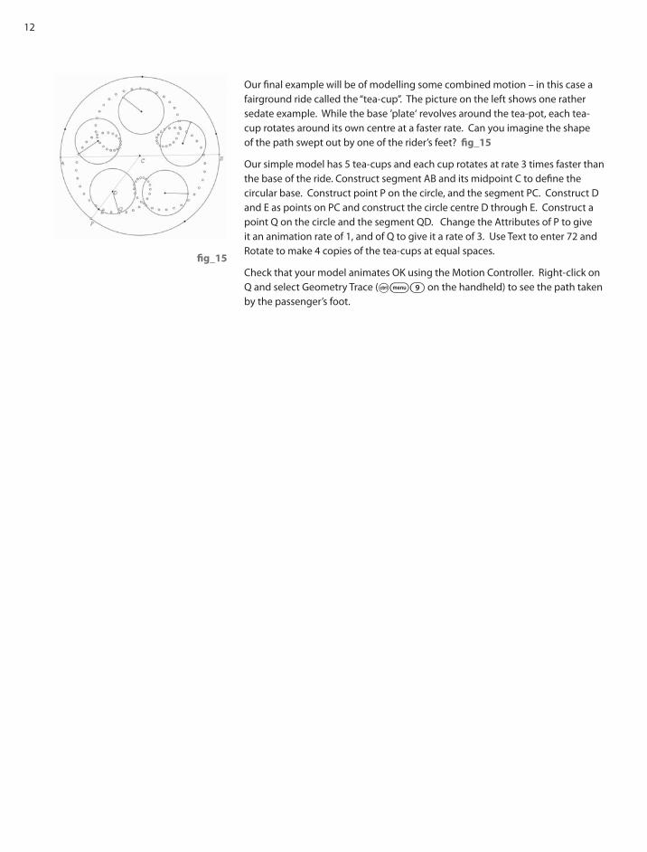
Our fi nal example will be of modelling some combined motion – in this case a

fairground ride called the “tea-cup”. The picture on the left shows one rather

sedate example. While the base ’plate‘ revolves around the tea-pot, each tea-

cup rotates around its own centre at a faster rate. Can you imagine the shape

of the path swept out by one of the rider’s feet? fi g_15

Our simple model has 5 tea-cups and each cup rotates at rate 3 times faster than

the base of the ride. Construct segment AB and its midpoint C to defi ne the

circular base. Construct point P on the circle, and the segment PC. Construct D

and E as points on PC and construct the circle centre D through E. Construct a

point Q on the circle and the segment QD. Change the Attributes of P to give

it an animation rate of 1, and of Q to give it a rate of 3. Use Text to enter 72 and

Rotate to make 4 copies of the tea-cups at equal spaces.

Check that your model animates OK using the Motion Controller. Right-click on

Q and select Geometry Trace (/b9 on the handheld) to see the path taken

by the passenger’s foot.

fi g_15


14

2Chapter

Morphing –

a change of shape,

size and/or position

15

We are used to seeing very sophisticated video clips where one face or object

steadily gets transformed into another, quite diff erent one. While these look

pretty tricky they all use some very simple mathematical principles, which

are performed many thousands of times in a very short interval to give the

impression of smooth changes. The underlying mathematics is based on

ratio. Very often we shall have need for a variable which runs just from

0 to 1. The name for such a variable is a parameter. The ‘meter’ part is

straightforward – it just means ‘a measure’. However ‘para’ has some quite

diff erent meanings – a ‘parasol’ is ‘against the sun’, as a ‘parachute’ is ‘against

a fall’. But a ‘paramedic’ is someone ‘acting like a doctor’, so it’s this meaning

which probably helps best – a ‘parameter’ is something ‘acting as a measure’.

In a new Geometry page hide the Scale (b27). Construct a segment AB

and place a point T on it. Measure the distances AT and AB using the measure

tool (b 8 1 on the handheld) and then select the length. Use the

Text tool (b16 on the handheld) to enter the expression ‘a/b’ (Use the p

key on the handheld for the ‘/’), and the Calculate tool (b 1 8 ·) on the

handheld) to substitute AT for ‘a’ and BT for ‘b’ in the expression by clicking on the

values when prompted.

On the diagram you can see I have used the text tool to add the text ‘t =’ to

the resulting value to make it clearer. As you slide T this should vary between

0 and 1. Where does t = 0.5 lie? By right-clicking (/b) on the points the style of

A and B have been set to be empty circles, and an animation speed has been

set for T – hence the appearance of the animation controller.

We now have the basic building block for many of the techniques to be applied

in this booklet. Remember that T is also an independent variable with the

segment AB as its domain – and we use it to compute the value of the variable

t which is a parameter with values between 0 and 1.

In our fi rst example we will apply some geometric transformations to translate,

rotate and enlarge a shape (polygon) smoothly. Construct a vector CD and

dilate (enlarge) about centre C the point D with scale factor the value of t to

obtain a point P on it (bB5· then click on C, then the number t

and fi nally D on the handheld). Construct a segment EF and use Compass

(bA7 on the handheld) to construct a circle centre P with EF as radius.

Construct a polygon whose vertices lie on this circle. Check that as you slide

T on AB, so P slides on CD, dragging the polygon and circle with it. So we’ve

cracked the translation (aka slide) bit!

Use the Text tool to enter numbers like 720 and 2 which will be used to control the

rotating and enlarging. Check that you have set the angle options in Document

Options for Degrees (not Radians). With the Text tool enter the formulae ‘c*d’ (Use

r on the hand held for ‘*’) and ‘1+e’. Use Calculate to substitute the value 720

for ‘c’, and that of ‘t’ for ‘d’. Check that as you slide T on AB so this result produces

numbers from 0 to 720, corresponding to performing two complete rotations in

the time T moves from A to B. Now use Calculate again to substitute the value 2

for ‘c’ and that of ‘t’ for ‘d’. Enter the formula ‘1+e’ and Calculate its value with the

last result substituted for ‘e’. Check that as you slide T on AB that this gives values

between 1 and 3, corresponding to increasing enlargement factors up to 3 times

in the time taken from T to move from A to B. All we now have to do is to perform


fi g_16

fi g_17

fi g_18

fi g_19

16

the two transformations and then do some tidying up!

Use the Rotation tool (bB4) to rotate the polygon (shown dotted) around

P as centre through the angle currently shown as 280°. Change the Attribute of

the resulting polygon to have a dashed perimeter.

Now use the Enlargement tool (bB5) to enlarge the rotated polygon with

centre P and scale factor currently shown as 1.78. Change the Attribute of this

polygon to shade it in. Now check that as you drag T on AB so the polygon

rotates and enlarges!

Finally you can hide all the unwanted clutter and use the Start Animation button

(which will appear when you click on T) to set it all in motion! It is best to kick it

off by fi rst dragging T over A before releasing it.

Making something grow in size is a standard technique to make it appear to be

coming towards you – i.e. to use perspective. Of course you may not want your

object to follow a straight line path – see if you can use the ideas from Section 1

to replace the vector CD with a curved arc on which P can run.

In order to suggest how changing shape is dealt with we shall use a very simple

pair of transitions fi rst to map the letter A to H and then to map it to P.

Start a New Problem with a Geometry sheet with the Scale hidden. The idea is

that we start with a letter A defi ned by some points and segments and fi nish

with a letter H. Since H needs 6 points and 5 segments and A needs 5 points and

5 segments we need to use a trick to defi ne A initially using two separate points

E and F quite close together and then drag them on top of each other once the

transitions have been tested.

Construct the A using points CDEFGH and segments CD, DE, DG, FG and GH.

Construct the H using points C’D’E’F’G’H’ and segments C’D’, D’E’, D’G’, F’G’

and G’H’.

Construct a slider T on a segment AB and use it to calculate the parameter t

between 0 and 1. This will be used to construct ‘in-betweenies’ like C’’ which

is the enlargement, centre C, of the point C’ with scale factor t. So use the

Enlargement tool by selecting the point C, then the Line Segment CC’ and fi nally

the calculated value of t, repeat this for each of the vertices to construct the

6 in-betweeny points like C’’ and hence the 5 in-betweeny segments forming

the shape which will morph from an A to an H. Check it works OK when you

slide T. Now you can set up the Animation, drag F on top of E and also hide any

unwanted bits.

Now we can construct a (rough!) letter P using 5 points and 5 segments. Next

we can set up 6 mappings between points on our current in-betweeny H and

the letter P. We are going to want the tops of the upward sticks of the H to come

together and join up, and also a point on the upper right stick of H to form into

the top right of the P – so create an additional point on the H as shown. Now

you can construct six segments such as C’’C’’’ (shown dotted) as the paths taken

by the points H as they morph to the P. Construct point C’’’’ on C’’C’’’ as the

Dilation of C’’’ with centre C’’ and scale factor t.

fi g_20

fi g_21

fi g_22

fi g_23


Repeat for the other 5 dotted segments. Join up the points for the new in-

betweeny (shown with medium weight segments). Check that as you slide T

on AB so the new shape closes itself up. Then you can hide all the messy bits

and check that the Animation button sets our shape on a path from A to P and

back again.

Try some more interesting shapes and paths to sharpen your morphing

and creative skills. As a fi nal example we will run through a pleasing kind of

kaleidoscope idea based on an equilateral triangle.

Start a new Problem with a Graphs page. Hide the axes and entry line. We

shall often use this as our main modelling page – because it allows us to plot

graphs of functions when and where we want and produces the same size page

when viewed in TI-Nspire software or on TI-Nspire handhelds. Check that you

have Degrees selected both as the Document option and also as the Geometry

angle. Construct points O, A, and the circle centre O through A. Construct the

intersection points D, E of the circle centre A through O with the fi rst circle.

Construct the intersection point B of the circle centre D through A with the

fi rst circle. Construct C similarly. Explain why ABC must be an equilateral

triangle (circles are very useful things when it comes to creating equal lengths!)

Construct the circular arc through D, O and E and a point P on it.

We now want to rotate P around O twice by 120° to obtain points Q and R.

Construct the polygon APBQCRA and check that it morphs from a hexagon

to a crossed over shape as you slide P. Finally hide all unnecessary clutter and

animate P on its arc DOE as domain.

Well now you have met some of the main ideas behind morphing. We need

to construct paths between each interesting pairs of corresponding points

AA’ in the starting and fi nishing objects. On each path we want to create an

in-between point A’’ which slides on the arc AA’ (which might be a segment,

or a circular arc, or part of a curve like those in section 1). We need to control

these in-between points so that they each perform their journey from starting

to fi nishing point in the same time. So we will either use one of them to

construct all of the others – as in the kaleidoscope idea above – or to have

them all controlled by a single parameter t as in the Dilation (aka enlargement)

approaches in the earlier examples.

Now it is over to you to see what creative juices fl ow as you construct your own

morphs. Good luck.

fi g_24

fi g_25

fi g_26

fi g_27

18

3Chapter

Smoothness –

circular arcs,

railway tracks,

eggs and ellipses

19

Below are some images which all have something in common – we are looking

at things often described loosely as “ovals”. Which would you say are the odd

ones out, and why?


The model railway track is made up from pieces which are either straight or

arcs of a circle. The British cyclist Bradley Wiggins was photographed in a time

trial in the 2009 Tour de France using an odd shaped front chain-ring – also

shown above in greater detail (http://www.osymetric.com/). The Brit Oval

cricket ground in London, the oval staircase in the US Supreme Court building,

and the Oval Offi ce in the White House (both in Washington DC, USA) do all

seem to share some common property. We know the London Eye must be

a circle, but why does the photograph make it look oval? The rugby ball is a

3D object formed by rotating an oval about its longer axis, as is an egg – but

are they the same shape? Certainly they all appear round, smooth and non-

circular – but there are distinct diff erences. This section is inspired by the book

Mathographics, Robert Dixon, Blackwell, 1987 – and it’s all about how to join

curves smoothly. It would help if you can imagine trains running along railway

lines, turning the handle-bars of a bike to round a bend, or changing direction

while skating or skiing. In each case, any change of direction needs to be done

smoothly in order to avoid disaster. In section 1 we met a piecewise defi nition of

a function and produced an animation involving some very unsmooth joins!

20

If you wanted to make a 90° change of direction on a railway track it would be

no good having two straight sections at right-angles to each other – you would

need a curve (probably an arc of a circle) of quite large radius to join them.

Let us see how this might work. Start a new Problem with a Graphs screen,

hide the axes and entry line, and set the angle modes to Degrees. Construct

Points A and B and the Line AB. Construct a Point C on AB, and use

Perpendicular to Construct a line through C perpendicular to AB. Construct

Points D and E on AB and the Segment DE. Construct Points F and G on the

perpendicular line, and the Segment FG. Can you see how we can draw a

circular arc through D and F to make a smooth join between ED and FG? What

do you know about tangents to circles? If the arc DF was to be a quarter of a

circle how would you fi nd its centre? fi g_28

Before we return to this problem we ought to have a new page to use as a

check-up on circles and tangents. Construct Points O and A, and the circle

centre O through A. Construct a point B on the circle, and the radius OB.

Construct the Tangent at B to the circle and a Point C on it. Measure the Angle

OBC. Remember this circle fact: the radius and tangent at a point on a circle

are perpendicular. Now construct two Points D and E on the circle. The segment

DE joining them is a chord of the circle. The tangents at D and E meet at F:

what sort of quadrilateral is ODFE?

Can you explain why DF and EF must be equal no matter what the angle DOE?

Construct the vector OF (b 7 8) and its Intersection G with the chord DE.

What is the relationship between DE and OF? In order to create a circular arc

we need to defi ne three points. Construct the Intersection H of OF with the

circle. Now you can use the Circular Arc tool (b79) with D, H and E to

defi ne the Arc DE of the circle. We have used some bold lines to emphasise the

‘bow and arrow’ shape associated with two points, their chord and their arc.

fi g_29

Returning to our original problem you must adjust D, C or F to ensure CD=CF

and then you can construct perpendiculars at D and F to locate the centre of the

circle which has DE as tangent at D and FG as tangent at F. Then you can use the

bow and arrow trick to construct the Arc joining D to F. Can you make it work?

A useful tool in TI-Nspire is called ‘Redefi ne Point’ (b19) fi g_30. So if we

construct the Circle centre C through D, then we can Redefi ne the point F to lie

on the intersection of the circle with the perpendicular at C.

The Perpendiculars at D and F meet at O, the centre of the circle which has FG

and DE as tangents. Using the bow and arrow construction we can Construct

the Vector OC and fi nd its Intersection H with the circle. Then we can Construct

the Circle Arc DHF. The smooth railway track is now shown in bold (/b3 then

adjust the line weight) as the path EDHFG. Can you imagine cycling along

it? What are you doing to the handlebars on ED, at D, on DHF, at F, and on FG?

Clearly there will be a maximum speed associated with each such circular curve

– the smaller the radius, the slower you can go. fi g_31

fi g_28

fi g_29

fi g_31

fi g_30

21

An alternative measure to the radius at a point is called the curvature at

the point, where curvature = 1/radius. In this way it makes sense to assign a

curvature of 0 to a straight line – and then the bigger the radius of a circular arc,

the smaller its curvature. Ideally we want small continuous changes in curvature

for a smooth ride – and we will learn more about these in the sections to come.

Before computer graphics became commonplace virtually every company which

produced objects had a ‘drawing offi ce’ where several ‘draughtsmen’ would

produce incredibly accurate drawings and ‘blueprints’ on drawing boards using

geometric instruments such as rulers, compasses, dividers and set squares. So

it was very important to be able to create curved objects using just these tools.

Also most machine tools for shaping wood, metal, plastics etc. could follow

straight or circular paths, but not more complex ones – and so it was important

to develop techniques for producing smooth curves using line segments and

circular arcs.

Robert Dixon is a computer graphic artist and a research fellow at the Royal

College of Art. One of Dixon’s recent claims to fame is in his accusations against

the artist Damien Hirst that he copied Dixon’s drawings. (http://www.dailymail.

co.uk/news/article-412263/Hirst-accused-plagiarism-artist.html ). In his book

Mathographics, he discusses a variety of ways of making drawings which model

the shapes of birds’ eggs. One of the simplest and most pleasing uses just 4

circular arcs and is constructed from a single segment AB.

fi g_32 is of an ‘Egg’ constructed by four smoothly joining circular arcs and

all based on the single line segment AB. fi g_33 gives a few clues about how

it was constructed. Study it carefully and see if you can work out how to do

the construction.

The clue lies in the two large circles. A circle is an important tool because all its

radii have the same length.

Here is one way to start the construction. On a clean page construct the

segment AB, its midpoint C and the circle centre C through A. Construct the

perpendicular bisector of AB and its intersections D and E with the circle.

Construct the circle centre B through A. Construct the ray from B through D to

meet the large circle in F. Construct the circle centre D through F. Construct the

ray AD and its intersection G with the smallest circle. Now you can see one of

the arcs BEA. Use the bow and arrow construction to help draw the arc AF. The

arc FG is easy to construct – just make an intersection point. fi g_34

The arc GB just requires a circle to be drawn through G and B, followed by the

bow and arrow trick. Then you can hide all the construction work just to show

the smooth outline of the ‘egg’. While the arcs join smoothly in the sense that

they have the same tangent either side of a join, there will be ‘jolts’ at A, F, G

and B if the shape was used as a rail track – at each of these points the radius

of curvature changes as you move from one arc to the next. This would mean

that the fl anges of the wheels would bump against the rails to stop the train

getting thrown off the track – and if the train was travelling too fast your coff ee

would shoot out of its container!


fi g_32

fi g_33

fi g_34

22

When you’ve done all the construction, measure the width of the ‘egg’ AB and

its length and hence fi nd the ratio of width to length. Measure some real eggs

(don’t go birds-nesting!) and see what sorts of ratios occur naturally. Invent

some diff erent ways of constructing eggs, or look up some on the Internet or in

Dixon’s book. Can you calculate the area enclosed by Dixon’s egg? How about

your own eggs?

This construction also known also as Moss’s Egg (http://mathworld.wolfram.

com/MosssEgg.html ).It is one of a family also known as Thom’s Eggs, after

the British engineer Professor Alexander Thom who invented them to model

Megalithic stone rings, like the ones at Cairnpapple Hill, Long Meg and

Castlerigg. fi g_35

The following information is extracted from the Amazon page on the book

“Alexander Thom: Cracking the Stone Age Code “ (Paperback) by Robin Heath,

Bluestone Press, 2007: http://www.amazon.co.uk/gp/product/0952615142.

“ Professor Alexander Thom was a foremost scientist and engineer of the last

century ... he had been Principal Scientifi c Offi cer for the design of the High

Speed Wind Tunnel at the Royal Aircraft Establishment, Farnborough, and

had assisted Sir Barnes Wallace in the design of the famous ‘bouncing bomb’

of `Dambuster’ fame. From 1934, Thom became interested in the megalithic

culture that had erected the stone circles, rows and other monuments

in Neolithic and Bronze Age Britain. He began to accurately survey these

sites, and in 1967 published “Megalithic Sites in Britain” (Oxford) where he

claimed the builders had been skilled surveyors and astronomers, and had

used an identical and accurate unit of length to mark out their constructions

throughout Britain, a length he called the Megalithic yard (2.72 feet or 0.829m).

Thom also discovered that they were using a geometry based on right-angled

‘Pythagorean’ triangles, triangles whose sides were whole numbers of this same

megalithic yard, or subdivisions or multiples of it.”

You can fi nd out more about his work on Megalithic culture at:

http://en.wikipedia.org/wiki/Alexander_Thom

http://www.dealbhadair.co.uk/athom.htm

http://www.megalithic.co.uk/article.php?sid=2146413596

Thom identifi ed two diff erent egg shapes for stone rings like those at Cairnapple

Hill in West Lothian and others in Devon and Cornwall (http://mathworld.

wolfram.com/ThomsEggs.html), each based on a 3,4,5 right-angled triangle.

See if you can construct his fi rst egg shape from the screen shot fi g_36.

See if you can locate a reference to the second egg shape which has 2 circular

arcs and 2 straight sections. fi g_37

“Long Meg and her daughter” in Cumbria is one of two of the “fl attened circle”

Megalithic stone shapes identifi ed by Thom. See if you can fi nd and construct

either or both of these.

fi g_37

fi g_36

fi g_35

23

So we have seen some techniques using circular arcs to construct smooth(ish)

curves. The next part of this section uses the ellipse as an example of a

smooth curve – one which is very important in science, as it describes the

paths followed by planets around the Sun and electrons around the nucleus

of atoms. While usually considered part of Advanced or Further Mathematics,

we can explore most of its properties using simple geometric techniques and

some trigonometry.

The following extract from an old book on construction techniques tells a

draughtsman how to draw an approximation to an ellipse. See if you can work

out how to carry it out in TI-Nspire. We will then see a way to draw an accurate

ellipse as a locus and check out how close a match it gives.

“ The four-centre method is used for small ellipses. Given major axis, AB,

and minor axis, CD, mutually perpendicular at their midpoint, O, draw AD,

connecting the end points of the two axes. With the dividers set to DO,

measure DO along AO and reset the dividers on the remaining distance to O.

With the diff erence of semi-axes thus set on the dividers, mark off DE along

DA equal to AO minus DO. Draw perpendicular bisector AE, and extend it to

intersect the major axis at K and the minor axis extended at H. With the dividers,

mark off OM equal to OK, and OL equal to OH. With H as a centre and radius R1

equal to HD, draw the bottom arc. With L as a centre and the same radius as R1,

draw the top arc. With M as a centre and the radius R2 equal to MB draw the

end arc. With K as a centre and the same radius, R2, draw the end arc. The four

circular arcs thus drawn meet, in common points of tangency, P, at the ends

of their radii in their lines of centres.”

Yes, a picture really is worth a thousand words! With TI-Nspire we use the

Compass tool (bA7), instead of the draughtsman’s dividers, to draw a

circle with a given centre and with a radius the same length as a given

segment. The fi gure below shows the full procedure. The four arcs meet in

pairs at the points P, Q, R and S – and in each case there is a change of curvature

at the join. fi g_40

The point P is the intersection of the upper arc, centre L and radius LP, with the

right end arc, centre K and radius KP, so there is quite a change in radius at P,

and hence curvature. fi g_41

In order to aid readability the screen shots are taken from the higher resolution

of the TI-Nspire software display, but all the constructions work fi ne on the

hand-held. In order to explore the actual curvature of a real ellipse we have got

to fi nd a suitable way of drawing one which will allow us to construct tangents.

Our fi rst attempt uses the construction called ‘auxiliary circles’.


fi g_38

fi g_39

fi g_40

fi g_41

24

On a new page construct a segment AB, its midpoint O and its perpendicular

bisector. Construct the point C on the bisector and refl ect it in AB to give the

point D. Construct the segment CD. Draw the circle centre O through A (the

major circle) and the circle centre O through C (the minor circle). Construct

a point X on the major circle and draw the segment OX. Construct the

intersection of OX with the minor circle as the point Y. Draw the line through

X parallel to CD and through Y parallel to AB. Construct their intersection point

Z. Check as you drag X on its circular domain so Z traces out a curve. Use the

Locus tool (bA6) to construct the curved path of Z as X slides on the major

circle. This locus is an ellipse. fi g_42

Unfortunately we cannot construct a tangent to the ellipse at the exact point

Z. Instead we can construct a point on the locus, draw its tangent and also the

perpendicular to the tangent through it (called the normal to the ellipse). If

we repeat this for another nearby point on the ellipse we will have two normals

which intersect in a point. The closer the points are on the curve, the nearer

the intersection of the normals is to the centre of curvature to the ellipse. Sadly

we can’t animate either point so we just have to drag each of them by hand to

a new position to see approximately how the curvature changes. In order to

animate the points we need to fi nd the equation of an ellipse.

The point Z on the ellipse has the x-coordinate of the point X and the

y-coordinate of the point Y. If the angle AOX is taken as the parameter t,

and the lengths OA = a, OB = b, then:

x = a cos(t) and y = b sin(t).

These are the parametric equations of the ellipse as t runs from 0° to 360°.

So, on a new Graphs page draw the ellipse as a parametric curve.

To construct this diagram begin by placing a point on the x-axis and fi nd its

co-ordinates (b17) and store the x-coordinate as a by clicking on the

x-coordinate and storing its value. Then repeat this putting a point on the y-axis

and storing the y-coordinate as b. Now you can plot the parametric equation of

the curve (b32) to change to parametric equation mode – and remember

to press r between a & cos(t) and b & sin(t)).

Now we can defi ne points P and Q on the curve, and YES we can animate them!

So again construct tangents and normals, and hence the approximate centre of

curvature. Give them both the same unidirectional animation speed of 1 and

pause the animation. Push P and Q very close together. Select Geometry Trace

for the point of intersection (b54). Now set the animation going, and

watch the approximate centre trace out a shape with four cusps – which is the

locus of the centre of curvature – and whose posh name is the evolute of the

ellipse. See how the shape changes as you slide B to change the eccentricity

of the ellipse. If OB = OA the ellipse becomes a circle, the radius of curvature

is the same everywhere, and there is a single centre of curvature for all points.

The eccentricity is measured by a number e = 1 – (b/a)2 which is zero for a circle

and approaches a maximum of 1 as b tends to zero.

fi g_42

fi g_43

fi g_44

fi g_45

25

The screens below show an experiment set up to capture data on the curvature

at P as the angle t sweeps from 0 to 360 (it uses some tricks you really do

not need to know about just now) – and the resulting graph shows how the

curvature moves smoothly between its minimum (straightest) and maximum

(sharpest) values. Of course, as b gets closer to a, so the ellipse gets closer to a

circle and the graph becomes a straight line – corresponding to constant radius.

Before we wrap this section up we will just have a look at a couple of properties

of the ellipse, which the ancient Greeks studied as a `conic section’. In the

picture alongside, the plane labelled π is a diagonal slice through a cone. It just

touches a smaller sphere at F and a larger sphere at F’. The cut face is an ellipse

having the two points F, F’ as foci. We shall see how they come into play.


fi g_46

fi g_47

fi g_48

fi g_49

26

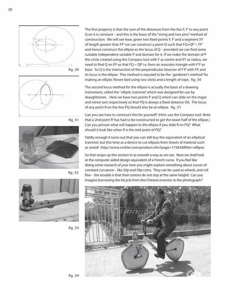
The fi rst property is that the sum of the distances from the foci F, F’ to any point

Q on it is constant – and this is the basis of the “string and two pins” method of

construction. We will see how, given two fi xed points F, F’ and a segment XY

of length greater than FF’ we can construct a point Q such that FQ+QF’ = FF’

and hence construct the ellipse as the locus of Q – provided we can fi nd some

suitable independent variable P and domain for it. If we make the domain of P

the circle created using the Compass tool with F as centre and XY as radius, we

need to fi nd Q on FP so that FQ = QP i.e. form an isosceles triangle with F’P as

base. So Q is the intersection of the perpendicular bisector of F’P with FP, and

its locus is the ellipse. This method is reputed to be the `gardener’s method’ for

making an elliptic fl ower bed using two sticks and a length of rope. fi g_50

The second locus method for the ellipse is actually the basis of a drawing

instrument, called the `elliptic trammel’ which was designed for use by

draughtsmen. Here we have two points P and Q which can slide on the major

and minor axis respectively so that PQ is always a fi xed distance OA. The locus

of any point R on the line PQ should also be an ellipse. fi g_51

Can you see how to construct this for yourself? (Hint: use the Compass tool. Note

that a 2nd point R’ has had to be constructed to get the lower half of the ellipse.)

Can you picture what will happen to the ellipse if you slide R on PQ? What

should it look like when R is the mid-point of PQ?

Oddly enough it turns out that you can still buy the equivalent of an elliptical

trammel, but this time as a device to cut ellipses from sheets of material such

as wood! http://www.rockler.com/product.cfm?page=17282&fi lter=ellipse

So that wraps up this section in as smooth a way as we can. Next we shall look

at the computer aided design equivalent of a French curve. If you feel like

doing some research of your own you might explore something about curves of

constant curvature – like 20p and 50p coins. They can be used as wheels, and roll

fi ne – the trouble is that their centres do not stay at the same height! Can you

imagine borrowing the bicycle from the Chinese inventor in the photograph?

fi g_50

fi g_51

fi g_52

fi g_53

fi g_54


28

4Chapter

Doing it with cubics

– Hermite splines

29

One of the techniques used in CAD is to produce a smooth shape controlled

by just a few points. Suppose for example we want to design an interesting

go-kart circuit. Assuming we want to make several laps, this will be a closed

curve – and, for safety’s sake, probably one that doesn’t intersect itself! You

can record a freehand curve using ICT in a number of ways e.g. by drawing

with a stylus on a tablet or Interactive Whiteboard and using the built-in

software to digitise the image – as a long list of pixel values. Similarly you

could draw on paper and use a digital scanner to produce a similar result.

You may have seen that such bitmap fi les can be very large. But they also are

‘dead’ in that once drawn we have no easy way of adjusting the shape, but

would have to use a photo editor, or Windows Paint software, to erase and/or

add pixels at a time – which is very tedious.

One feature of many drawing packages, including the last version of Microsoft

Word in Offi ce 2007, is the facility to create a smooth curve controlled by just a

few mouse clicks. In Word, choose the Insert (2nd) tab, and then Shapes from

the Illustrations tab. This produces a table of diff erent tools. Look at those under

the Lines heading and choose the 10th option called Curve whose symbol looks

like a segment of a cubic curve with a maximum and minimum. Now you can

click anywhere with the mouse to start drawing, and then each time you move

and click again you get a segment of a smooth curve. Fifteen points were used

to make the shape below, and when the 16th click was made on, or very close to,

the 1st point, the software closes up the curves and gives you a fi nished graphic

object. Try it for yourself. If you right-click in the graphic area, the 4th menu

off ering is Edit Points, and you will see exactly where the 15 points are located.

You can move points, delete them, add more ones etc.. So that tool has the

features we would like to have in designing the go-kart track.

fi g_55

The design fi g_56 uses just 7 diff erent points, and closes back to the starting

point. So the curve is actually made up from 7 curved arcs each of which joins

its neighbours smoothly at the end points. By changing the position of just one

control point (the red blob), shown by the before and after closed curves, we

have local control. This means that only a few of the arcs nearest to that control

point are aff ected.

fi g_56


30

Each arc is uniquely determined by the position of its end-points and the

tangent vectors at the joins with its neighbouring arcs. Instead of using the

graphs of seven cubic functions it gives more fl exibility if we represent each arc

by a parametric curve – with both x and y as polynomials in the parameter t.

The mathematical detail

(apparently not for the faint hearted, but not really that hard!)

Each polynomial will have just 4 degrees of freedom – since it must match the

x-coordinates of its two end-points, and also match the gradients at its end

points with the x-components of the tangent there. So we can look for a cubic

polynomial like x(t) = p + qt + rt2 + st3 – and arrange for t=0 to correspond with

the starting point A, and t=1 with the fi nishing point B – so the domain of t for

the arc AB is the interval 0 ≤t≤1. The nice thing about cubic functions is that

they can include infl ections (i.e. wiggles)!

Since the arc joins points A (ax,ay) and B (bx,by) and has tangents with

components [atx,aty] and [btx,bty] at A and B, then we should be able to make

life easier by writing the equation of the arc in the special form:

x(t) = p(t).ax + q(t).bx + r(t).atx + s(t).btx , y(t) = p(t).ay + q(t).by + r(t).aty + s(t).bty , 0 ≤t≤1

In this case we will look for four cubic polynomials for our coeffi cients, rather

than four constants. Then both x(t) and y(t) will be linear combinations of

the four basic polynomials and every arc will have a similar form – all we have

to do is to change the values like ax, bx, atx and btx. In fact these four basic

cubic functions of t are called the Hermite cubic spline curves after the French

mathematician Charles Hermite (1822-1901). You can fi nd out more about

them at: http://en.wikipedia.org/wiki/Cubic_Hermite_spline. We will now

fi nd equations for each of them.

If we take t = 0 then we should be at A, and then x(0) = ax and y(0) = ay.

A simple way to ensure this is if p(0) = 1 and q(0) = r(0) = s(0) = 0.

Can you see why t must then be a factor of q(t), r(t) and s(t)? Cunning, eh?

Also when t = 1 we are at B, so x(1) = bx.

Again we would like q(1) = 1 and p(1) = r(1) = s(1) = 0.

In this case (1-t) must be a factor of p(t), r(t) and s(t) – agreed?

Diff erentiating with respect to t and writing e.g. we have:

x’(t) = p’(t).ax + q’(t).bx + r’(t).atx + s’(t).btx and similarly for y’(t).

Again we look what happens when t = 0, and when t = 1.

Since x’(0) = atx we need r’(0) = 1 and p’(0) = q’(0) = s’(0) = 0.

So t must be a factor of p’(t), q’(t), s’(t).

Also x’(1) = btx , so s’(1) = 1 and p’(1) = q’(1) = r’(1) = 0 and (1-t) must be a factor

of p’(t), q’(t), r’(t).

= x’(t)dx(t)

dt

31

Can you show why if (1-t) is a factor of both p(t) and p’(t) then (1-t)2 must be a

factor of p(t)?

Similarly if t is a factor of q(t) and q’(t) then t2 must be a factor of q(t).

This gives us most of the information we need about our four polynomials:

p(t) = (1+d.t)(1-t)2

q(t) = (1 + e.(1-t))t2

r(t) = f.t(1-t)2

s(t) = g.t2(1-t)

We just need to fi nd the values for d, e, f and g.

See if you can suggest how we might fi nd them.

The screen shot below shows an approach using TI-Nspire CAS.

fi g_57


32

So we fi nd that d = 2, e = 2, f = 1 and g = -1

agreeing with the equations given in Wikipedia!

Plotting graphs of each of the functions:

p(t) = (1+2t)(1-t)2

q(t) = (3-2t))t2

r(t) = t(1-t)2

s(t) = -t2(1-t)

we can also see the behaviour in the interval 0 ≤t≤1

again in agreement with Wikipedia.

So armed with our 4 basic cubic splines we are ready to go forth and draw

mathematical fl exi-curves. fi g_58

But what is a spline? The term dates from the days when draughtsmen made

detailed technical drawings of objects on a large drawing board. To “fair a

smooth curve” they had long strips of steel or laminated wood, and sets of

heavy weights, called ‘ducks’. By adjusting the number and position of the

ducks they could make the spline follow the desired path, which could then

be traced. By recording the position of each duck they could ensure that they

could reproduce the curve if needed. So the challenge to the mathematician

was to produce the mathematical equivalent of the physical spline. fi g_59

fi g_58

33

The fi le Hermite.tns shows how we can start to build up each segment of a

curve using 8 pieces of data: the coordinates of the ends A,B and the

components of the tangent vectors tA and tB. The points and vectors are

constructed in a Graphs page.

Using Coordinates and Equations we can fi nd the coordinates of the 4 points

used. With a right-click on the x-coordinate of A we can store it as the variable

ax, and similarly we can defi ne ay, bx and by. Writing the text “p-q” on the screen

we can use Calculate to feed it in turn with the values of the coordinates of the

beginning and end of each vector to calculate the tangent components, which

we store as atx, aty, btx and bty. These values are copied into the Spreadsheet,

where e.g. A1 = ax, B1 = ay, C1 = atx and D1 = aty. The basic cubic splines are

defi ned in the Calculator window, and used to defi ne the parametric equations

for the arc AB. This leaves A in the direction of the tangent tA, and enters B in

the direction of the tangent tB. For the confi guration shown, the arc has an

infl ection. Using ‘Point On’, the point P is constructed on the arc and its Tangent

is also constructed. Using a right-click on P, its Attributes can be adjusted to

give an animation speed of 3 unidirectionally along AB. Click on the green

Play button to start the animation. fi g_60

fi g_59


fi g_60

34

For a single arc, the spreadsheet is not actually needed. But if each new

point has its own row, then the data for the 4th arc, say, will come from rows

4 and 5. So instead of referring to dx and ex, say, we can call them xc[4] and

xc[5] – and that allows us to write the general form of the parametric equations

using lists as, say:

xh(k,t) = p(t).xc[k] + q(t).xc[k+1] + r(t).xt[k] + s(t).xt[k+1]

yh(k,t) = p(t).yc[k] + q(t).yc[k+1] + r(t).yt[k] + s(t).yt[k+1].

So now we can see the eff ect of adding an extra point C and tangent tC. fi g_61

fi g_61

The important things about this model for a fl exi-curve are that:

(a) the fi nished curve passes through all the control points

(so it interpolates the points);

(b) the curved arcs join smoothly at the control points,

having a common tangent;

(c) the arcs themselves are also smooth,

and fl exible enough to allow for infl ections.

So here is a more complex version using the same principle but having seven

control points. In order to create a closed curve, an 8th row has been added

which is a duplicate of the fi rst row.

The user interface has been designed so that you can change the position

of each control point, the direction of its vector and the magnitude of that

vector independently.

So, even if the mathematical detail was a closed book, you now have a

modelling tool to work with! fi g_62


fi g_62

However, the fl exi-curve used in Word only required the user to specify the

control points, not the vectors. So it must use some technique (or algorithm)

to calculate the vectors based on the geometry of the control points. We can

only guess what this is, but the underlying polygon ABCDEFG might yield a

clue. Suppose we fi nd the midpoints of each segment e.g. let A’ be the midpoint

of AB etc.. Then for the points ABC, the vector A’B’ might be a reasonable choice

for the direction vector at B, and so. Let’s test this out. We can construct each

midpoint vector like A’B’ and use it to translate each control point like B to B’’.

Then the vector BB’’ will be a reasonable choice for the tangent at B. So we

can drag our test points to lie over the new positions, like B’’, to see if we get a

reasonable shape. fi g_63

fi g_63

fi g_64 fi g_65

Now that looks to be OK we can redefi ne our old ‘compass’ vectors to have their

endpoints at the new B’’ style positions. fi g_64

Now that’s worked OK, we can use Hide/Show to tidy things up. fi g_65

36

The problem with redefi ning the points to defi ne the vectors is that now we

have lost the means of changing the stored variables atx, aty etc.. So changing

positions of the control points is no longer updating the spreadsheet as we

would like. But that’s no problem! Given the coordinates of the control points

stored in the columns xc and yc of the spreadsheet we should be able to

compute all we need. As a fi rst step we can introduce additional columns xm

and ym to hold the coordinates of the midpoints like A’. Then using these we

can calculate the vector components xt and yt. fi g_66

However, we can also fi nd the values for the cells in xt and yt directly from those

in xc and yc without the explicit calculations for xm and ym: fi g_67

Consider cell C2 = e2 – e1 = (a2+a3)/2 – (a1+a2)/2 = (a3-a1)/2

So that’s the typical formula, but we need to handle the ‘wraparounds’:

C1 = (a2-a7)/2 = C8.

Now we eff ectively have the equivalent of the Word fl exi-curve in the Graphs

page, but also in the Lists & Spreadsheets and the Calculator views we also have

on show the algorithm that Word is using behind the scenes! As you move any

control-point you should now see just a few of the spreadsheet entries changing

– showing ‘local control’. fi g_68

fi g_66

fi g_68

fi g_67

fi g_69

37

The Wikipedia mentions something called the ‘cardinal spline’. In fact we have

already just done this for the case c = 1 – and we can easily model the general

case by adjusting values within the spreadsheet. We don’t have to do what

we’re told! So the slider has been set up to explore the eff ects of values of

c between -2 and 3.

Now we can also explore changing the tension parameter c. fi g_69

Here are some things you might like to follow up

Ex. 1: Make an interesting go-kart circuit using 7 points.

Ex. 2: Trace round a shoe (or use an insole) and see if you can model the

resulting shape using just 7 points.

Ex. 3: Create one or more additional points and vectors, also creating extra

variables, rows of the spreadsheet and parametric arcs and use it to

design more complex curves.

Ex. 4: Find out more from the Wikipedia reference (and by your own searches)

about other ways of computing the vectors from the coordinates to give

the equivalent of the way Word draws the curves without being told the

tangent vectors and write or adapt TI-Nspire fi les to investigate them.

Ex.5: Find out more about Edwin Catmull and his mathematical contributions

to the world of fi lm and video.

Ex.6: Find out about the radius of curvature of a curve, and explore whether

or not our cubic Hermite splines always give the same radius of curvature

at each side of a control point. This would be an important consideration

in designing roads, railways etc.. Can you fi nd out (or maybe invent) a

technique for the calculation of the vectors at the joins to give continuity

of position, tangent and curvature?

Ex.7: Find out how to compute the length of a parametric arc between

t = 0 and t = 1 and hence compute the total arc length of a closed

cubic-spline curve.


38

5Chapter

Doing it with cubics

– B-splines


We’ve already met most of the key ideas we need - B-splines just provide

a neat way of sewing them together. As with the Hermite curves, we will

make a smooth curve by joining together a set of cubic arcs. We will also use

four pieces of information, but this time we will use the coordinates of four

successive points like A, B, C and D. The x-coordinates of a point T on the arc

will be a weighted average (a blend) of the four x-coordinates, and similarly

for the y-coordinates. As with Hermite, the curve could be in 3D (or higher

dimensions) by taking z-coordinates as well. Also the curve could be open

or joined up (as with a race-track). We just need to know what the weighting

functions will be. While they are not quite as obvious as the Bézier weighting

functions they are relatively straightforward polynomial functions.

First, take a step back and see what a quadratic arc formed by 3 points

A, B and C looks like. The functions we are going to use are:

f(t) = ½ (1 – t)2

g(t) = ½ + t(1-t)

h(t) = ½ t2

where the parameter, t, runs from 0 to 1. Check that f(t) + g(t) + h(t) = 1

for all values of t.

We will also take the opportunity to see fi rst how we can make an algorithm

explicit in a spreadsheet.

If A has coordinates (ax, ay) etc.., then the coordinates of any point T will be

given by the equations:

tx = f(t) ax + g(t) bx + h(x) cx

ty = f(t) ay + g(t) by + h(x) cy

We just need to convert the algebraic formula into a version the spreadsheet

“understands”.

If d3 represents the contents of the cell D3, we can use the “$” symbol to fi x

either the column reference “d” or the row reference “3” or both: e.g. $d3, d$3 or

$d$3. These notations are called absolute, rather than relative, references and

are important when fi lling cells across a row or down column.

40

Here is a spreadsheet set up to generate 17 points on the quadratic arc with

values of t from 0 to 1 in increments of 1/16 (as with a For-Next loop in a

programming language). fi g70

The formula in cell G1 is: g1 = $d1*a$1 + $e1*a$2 + $f1*a$3

When copied down this becomes: g2 = $d2*a$1 + $e2*a$2 + $f2*a$3

And when copied across we get: h1 = $d1*b$1 + $e1*b$2 + $f1*b$3

fi g_70

We can display the results graphically in either a Data & Statistics page or a

Graphs page.

The arc looks quadratic, but in the sense of a rotated parabola rather than

either a quadratic regression function or a manipulated quadratic function.

Try dragging A, B and/or C around so that the axis of the arc is (nearly)

horizontal, or is diagonally inclined. Hence we cannot, in general, express

the curve as a simple function of x, but our equations for T (tx, ty) defi ne the

locus of T in terms of the graph of parametric equations.

fi g_71 fi g_72


Now we see how the cubic arc is related to the quadrilateral defi ned by the four

control points A, B, C and D.

So, if we have, say, 5 points we can fi nd a fi rst arc controlled by ABCD, then a

second arc controlled by BCDE etc.. Or we could complete a closed arc in the

quadrilateral by computing arcs controlled by ABCD, BCDA, CDAB and DABC etc..

We can perform the whole task in a Graphs page. First three points A, B and

C have been constructed, their coordinates displayed, and each coordinate

stored in a variable, such as ax. Now the three functions f1(x), f2(x) and f3(x)

can be defi ned as Function Graph Plots, but then their graphs are hidden.

Finally we can defi ne a Parametric Graph Plot by the function displayed on the

screen. In the defi nition screen we also fi xed the value of the parameter t to be

between 0 and 1 with an increment of 1/16. Check that you can now move A,

B and C around and explain the geometric relationship between the quadratic

parametric arc and the triangle ABC.

Having gone back to quadratics we can now step forward again to cubics.

We just need an extra point D and an extra weighting function f4(x). We also

need new defi nitions for all four weighting functions which are:

f1(t) = 1/6 (1 – t)3

f2(t) = 1/6 ((2 – t)3 – 4(1 - t)3)

f3(t) = 1/6 ((1 + t)3 – 4 t3)

f4(t) = 1/6 t3

fi g_73 fi g_74

42

So now you have been inducted into the dark secrets of the computational

geometry which has been developed over many years initially to aid designers

and engineers, but now increasingly in the entertainment industry for cartoons,

animations and computer games.

We have not (yet) gone into techniques for using colour, such as rendering,

nor to explore the wide world of three dimensions. They will have to wait for a

future book – watch this space!

fi g_75 fi g_76


1

TI-Nspire™ is a trademark of Texas Instruments. All trademarks are the property of their respective owners.

Texas Instruments reserves the right to make changes to products, specifi cation, services and programs without notice.

© 2010 Texas Instruments

STEM activities with TI-Nspire

The coming decade will see an increasing need for a

fl exible work force possessing a wide range of skills in

Science, Technology, Engineering and Mathematics

(STEM) in order to meet the needs of the new high level

industries and to be able to produce technologically

complex products. The booklets in this series were

developed with this need in mind. They aim to provide

stimulating activities which link aspects of STEM and

at the same time encourage the use of technology

and an awareness of its potential.

Why use TI-Nspire for STEM subjects?

TI-Nspire provides a learning platform which dynamically

links a variety of ICT applications including documents,

graphs, geometry, statistics, spreadsheets, data logging

and a calculator. This dynamic linking assists students in

making connections not only between diff erent areas of

mathematics but also with other areas of the curriculum

and STEM subjects in particular.

There is now a wealth of data available on the Internet

in a variety of forms which can be copied directly into

TI-Nspire. Data can also be captured by linking to a variety

of data logging devices such as motion sensors or by

recording manually or using video analysis. It is then

possible to manipulate, display and analyse this data

in a variety of ways or to try to model the data using

a variety of data handling and function plotting tools.

About the booklets

All the activities contain some background scientifi c

or other information together with links to appropriate

websites. Many of the activities are suitable for a range

of ages and aptitudes with more challenging ideas being

suggested as extension activities. Further information

and TI-Nspire fi les for the activities can be found at

www.nspiringlearning.org.uk.

There are fi ve booklets in the series:

Introduction - contains a brief introduction and

instructions for getting started using some of the features

of TI-Nspire that are used frequently in the other booklets.

Capturing data: Modelling and Interpretation - contains

activities which use a variety of data logging probes to

collect real data and analyse it further.

Using real world data - contains activities which investigate

and analyse data in a variety of ways from ready-made or

easily generated data sets in a variety of contexts.

Mathematics in motion - contains investigations into

modelling motion based on diff erent forms of data

collection: manual, video and data logging.

Computer graphics - brings together a number of

diff erent mathematical approaches which are used by

computer programmers to create and manipulate images;

techniques that have now found their way into “virtual

reality”. These activities make use of TI-Nspire applications

especially Graphs and Geometry.

Documents

Computer Graphics - Texas Instruments