Computer Forensics using Bayesian Network: A Case Studyi.cs.hku.hk/~cisc/forensics/papers/BayesianNetwork.pdf · - 2 - I. INTRODUCTION The proliferation of computer crimes has driven

- 1 -

Computer Forensics using Bayesian Network: A Case Study

Michael Y.K. Kwan, K.P. Chow, Frank Y.W. Law, Pierre K.Y. Lai {ykkwan,chow,ywlaw,kylai}@cs.hku.hk

The University of Hong Kong

Abstract

Like the traditional forensics, computer forensics involves formulation of hypotheses grounding on

the available evidence or facts. Though digital evidence has been statutory witnesses for a span of

time, it is a controversial issue that conclusions drawn from revealed digital evidence are subjective

views without scientific justifications. There is an escalating perception that computer forensics is just

the subjective conclusion of computer professionals.

The purpose of this paper is to present a reasoning model based on the probability distribution in a

Bayesian Network. By setting out probability distributions over hypotheses for computer forensics

analyses, we hope to quantify the evidential strengths of such hypotheses, and thereby enhance the

reliability and traceability on the analytical results of computer forensics examinations. To study the

validity of the proposed model, a real court case about BT technology has been fitted to the

calculations. In order to detach the subjective views, a survey was carried out to collect the expertise

of 31 experienced law enforcement agencies. Their responses were aggregated to generate some more

objective assignments to the prior probabilities to be used. The outcome demonstrates a high

propagated probability of 92.7%, which is in accordance with the actual court verdict of guilty. That

presents computer forensics a real scientific science with quantifiable analyses.

Keywords: Bayesian Network, digital evidence, prior probability

- 2 -

I. INTRODUCTION

The proliferation of computer crimes has driven the need for the analysis of digital evidence.

As forensic science has long been used to resolve legal disputes regarding different branches of

science, computer forensics is developed naturally in the aspects of computer crimes or

misbehaviours.

Similar to other forensics taxonomies, computer forensics involves the formulation of

hypotheses that are based on available evidence or facts and the assessment of their likelihood that

support or refute the hypotheses. Although there are principles and guidelines established on how to

retrieve digital evidence [14,15,16], there seems lack of researches on the evaluation of the accuracy

of the established hypotheses. To reach persuasive forensics conclusions, computer forensics

analyses require reliable, accurate and scientific methodologies to justify their hypotheses.

Without reliable and scientific analytical models, computer forensics analysts are facing the

challenges of unjustified forensic conclusions or that the findings are speculations without concrete

scientific support. It also renders forensic results varies from analyst to analyst. These contrasting

interpretations will bring different analysts resulting in contradictory conclusions even given the same

set of digital evidence.

Today, this shortage has drawn impacts on the reliability of the forensics findings as well as

the credibility of the analyst. Speculations or subjective views of forensic analyst under the name of

expert opinion are no longer sufficient for legal arguments [1].

The purpose of this paper is to present a reasoning model based on the probability distribution

in a Bayesian Network. The model is expected to provide scientific justifications for the conclusions

or findings of computer forensics examinations. This model is developed to facilitate other computer

forensics practitioners to trace and to assess events or parameters of the examinations such that the

reasoning for the conclusions can be evaluated.

- 3 -

II. LITERATURE REVIEW

Forensics is the process of analysis and interpretation of evidence so as to determine the

“likelihood” of a crime. Many researchers revealed that this process should cover the formulation of

hypotheses from evidence and the evaluation of the hypotheses’ likelihood for the sake of legal

arguments in court proceedings [2, 3, 4, 5, 6]

Aitken and Taroni [7] viewed that likelihood is indeed an exercise in hypothetical reasoning.

It denotes the degree of belief on the truthfulness of the hypothesis. In the scientific community,

likelihood is expressed in terms of probability. As probability is the logic of chance, hence

probability theories are able to deduce the likelihood of hypotheses from assumptions.

Although probabilistic methods seem to be viable measures to prove or refute the hypotheses

of a crime, it is viewed by Jones et al [8] that simply obtaining all possible probability distributions

on the entailing evidence of a crime are not practical. Given that the volume of evidence of a crime is

usually large, the effort to obtain the joint probability distributions for all possible evidential variables

is therefore very large and expensive. Moreover, since simple probabilistic methods cannot reflect

any of the conditional dependencies between the evidence, these methods are considered impractical

from an analytical point of view [9]. From researches, it was concluded that a more structural

probabilistic model should be used in order to provide a more efficient and representation of the

conditional dependencies of evidence [9,10,11].

Indeed, crime investigation should be considered as an abductive diagnosis problem [10].

However, it is difficult to design a model that can deterministically describe all the assumptions of a

crime. Poole [12] therefore proposed a model that can describe crime scenarios non-deterministically

using symbolic logic and probabilistic Bayesian methods. However, the profound model proposed by

Poole [12] is considered too abstract to be applied in real scenario.

Furthermore, digital events are discrete computer events that are deterministic and in temporal

causal sequence. Therefore, it is a prevailing practice that computer forensic analysts will establish

- 4 -

their abductive reasoning based on the existence or validity of the causation events that entailing the

hypotheses. However, it is difficult to have consistent models to determine the supporting events for

hypotheses. Different analyst may attach different events for the same hypothesis. Even if the same

set of events is determined, analysts may assign different probabilistic values to the events. This is

referred as the subjective probability.

Moreover, analysts are facing the challenge of uncertainty in forming their reasoning when

certain evidential events of the hypotheses are found missing or uncertain. This uncertainty also

causes difficulties for computer forensics analysts to evaluate the remaining events. On one hand,

these remaining events cannot prove complete truthfulness of the hypotheses, whilst on the other,

these events indicate a certain extent of likelihood of the hypotheses.

In this paper, we propose the usage of the Bayesian Network model to evaluate digital

evidence and to handle evidential uncertainties in reasoning formulation. Furthermore, in order to

obtain a more objective prior probability or measurement of belief for events that are believed to be

caused by the hypotheses, statistical data on the probabilistic values of a number of digital forensics

scenarios are gathered from computer crime investigators and computer forensics examiners through

questionnaires.

III. OVERVIEW OF BAYESIAN NETWORK

Before we explore the Bayesian network, it is worthwhile to emphasis that digital evidence is

indeed “past” event that was caused by the hypothetical event. For example, the suspect had

downloaded some child-pornographic materials from a pornographic web site and the URL of the

web site was then recorded on the Internet history file.

A Bayesian Network is a graphical model that applies probability theory and graph theory to

construct probabilistic inference and reasoning models. The nodes represent variables, events or

evidence, whilst the arc between two nodes represents conditional dependences between the nodes.

- 5 -

A Bayesian Network is defined as a Directed Acyclic Graph (DAG) in which the arcs are

unidirectional and feedback loops are not allowed in the graph. Because of this feature, it is easy to

identify the parent-child relationship or the probability dependency between two nodes.

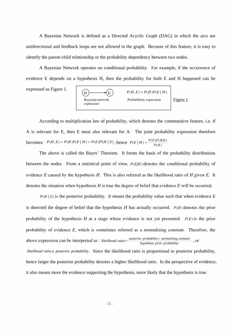
A Bayesian Network operates on conditional probability. For example, if the occurrence of

evidence E depends on a hypothesis H, then the probability for both E and H happened can be

expressed as Figure 1.

According to multiplication law of probability, which denotes the commutative feature, i.e. if

A is relevant for E, then E must also relevant for A. The joint probability expression therefore

becomes: , hence

The above is called the Bayes’ Theorem. It forms the basis of the probability distributions

between the nodes. From a statistical point of view, P(E|H ) denotes the conditional probability of

evidence E caused by the hypothesis H. This is also referred as the likelihood ratio of H given E. It

denotes the situation when hypothesis H is true the degree of belief that evidence E will be occurred.

P(H | E) is the posterior probability. It means the probability value such that when evidence E

is detected the degree of belief that the hypothesis H has actually occurred. P(H ) denotes the prior

probability of the hypothesis H at a stage where evidence is not yet presented. P(E) is the prior

probability of evidence E, which is sometimes referred as a normalizing constant. Therefore, the

above expression can be interpreted as : , or

. Since the likelihood ratio is proportional to posterior probability,

hence larger the posterior probability denotes a higher likelihood ratio. In the perspective of evidence,

it also means more the evidence supporting the hypothesis, more likely that the hypothesis is true.

P(H , E) = P(H )P(E | H ) = P(E)P(H | E) P(E | H ) = P(E )P(H |E )

P(H )

P(H , E) = P(H )P(E | H )H E

Bayesian network expression

Probabilistic expression

posterior probability normalizing constanthypothesis prior probability

likelihood ratio = ×

likelihood ratio posterior probabilityα

Figure 1

- 6 -

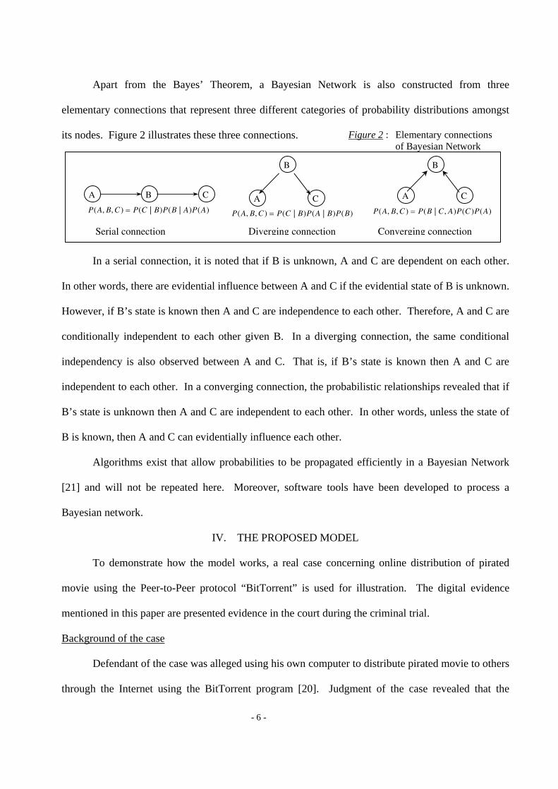
Apart from the Bayes’ Theorem, a Bayesian Network is also constructed from three

elementary connections that represent three different categories of probability distributions amongst

its nodes. Figure 2 illustrates these three connections.

In a serial connection, it is noted that if B is unknown, A and C are dependent on each other.

In other words, there are evidential influence between A and C if the evidential state of B is unknown.

However, if B’s state is known then A and C are independence to each other. Therefore, A and C are

conditionally independent to each other given B. In a diverging connection, the same conditional

independency is also observed between A and C. That is, if B’s state is known then A and C are

independent to each other. In a converging connection, the probabilistic relationships revealed that if

B’s state is unknown then A and C are independent to each other. In other words, unless the state of

B is known, then A and C can evidentially influence each other.

Algorithms exist that allow probabilities to be propagated efficiently in a Bayesian Network

[21] and will not be repeated here. Moreover, software tools have been developed to process a

Bayesian network.

IV. THE PROPOSED MODEL

To demonstrate how the model works, a real case concerning online distribution of pirated

movie using the Peer-to-Peer protocol “BitTorrent” is used for illustration. The digital evidence

mentioned in this paper are presented evidence in the court during the criminal trial.

Background of the case

Defendant of the case was alleged using his own computer to distribute pirated movie to others

through the Internet using the BitTorrent program [20]. Judgment of the case revealed that the

A B C

P(A, B, C) = P(C | B)P(B | A)P(A)A

B

C

P(A, B, C) = P(C | B)P(A | B)P(B)

A

B

C

P(A, B, C ) = P(B | C, A)P(C)P(A)

Serial connection Diverging connection Converging connection

Figure 2 : Elementary connections of Bayesian Network

- 7 -

defendant was in possession of optical disc of the movie. To achieve the distribution act, the

defendant copied the movie from the optical disc onto his computer. He then used the BitTorrent

program to create a torrent file from the movie file. Torrent file contains meta-date of the source file

(i.e. the movie file) and the URL of the Tracker server. It can facilitate other Internet users to join the

Peer-to-Peer network.

To make it available for other users, the defendant sent the torrent file to various newsgroup

forums. He thereafter activated the created torrent file on his computer, which rendered his computer

connected to the Tracker server. When connected, the Tracker server would query the computer with

regard to the meta contents of the torrent file. The Tracker server would then return a peer list

showing existing IP addresses on the network and the percentage of the target file existed on each

peer machine.

Since the defendant’s computer had a complete copy of the movie, hence the Tracker server

would label it as seeder computer. Finally, the defendant maintained the connection between the

Tracker server and his computer so that other peers could download the movie from his computer.

Building the model

Constructing a Bayesian model for computer forensics analysis begins with the set up of the

top-most hypothesis. Usually, this hypothesis represents the main argument that the analyst wants to

determine. For the purpose of prove the alleged illicit act, the hypothesis to be used is :

Hypothesis H : “The seized computer was used as the initial seeder to share infringing file on

a BitTorrent network”

Then we have to express the hypothesis’s possible states, which indeed denote the possible

findings of the hypothesis. In the case, the possible states of the hypothesis are : “Yes, No,

Uncertain”. It is also required to assign the probability values to these three states. These values are

also known as prior probability of the hypothesis.

- 8 -

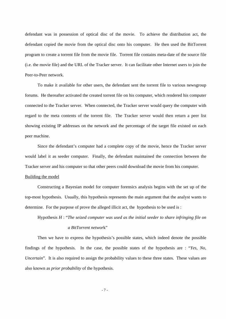
The hypothesis H is the root node without any parent nodes. Indeed, node H is an ancestor of

every other node in the Bayesian Network, hence its states’ probabilities are unconditional. Until the

states of the child nodes of H are certain, the probabilities of H should be evenly distributed amongst

its states. Therefore the probability of H is P(H) = (0.333, 0.333, 0.333)

Having established the root node, we then move to explore evidence or events that are causally

dependent on H. These evidence or events are usually observable variables. However, it is noted that

sub-hypotheses may also added under the root node of a Bayesian network. Although these sub-

hypotheses are not having observable states, they are useful because they can refine the resultant

model to a more structural and clearer graph. To support the hypothesis, that is “The seized computer

was used as the initial seeder to share infringing file on a BitTorrent network”, the following five sub-

hypotheses are created:

(1) 1H : The pirated file was copied from the seized optical disc, which was found at the scene of

crime, to the seized computer (states : “Yes, No, Uncertain”);

(2) 2H : A torrent file was created from the copied file (states : “Yes, No, Uncertain”);

(3) 3H : The torrent file was sent to newsgroup forum for publishing (states : “Yes, No, Uncertain”);

(4) 4H : The torrent file was activated, which rendered the seized computer connected to the Tracker

server (states : “Yes, No, Uncertain”); and

(5) 5H : The connection between the seized computer and the Tracker server was maintained (states :

“Yes, No, Uncertain”).

At this point, since the sub-hypotheses are dependent on H, we need to assign conditional

probability values to these sub-hypotheses.

Node Name H State Yes No Uncertain

Prior probability P(H) 0.333 0.333 0.333

H

Root node of Bayesian network

Table 1

- 9 -

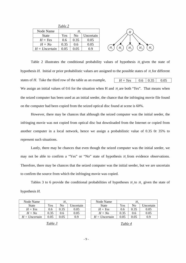
Table 2 illustrates the conditional probability values of hypothesis 1H given the state of

hypothesis H. Initial or prior probabilistic values are assigned to the possible states of 1H for different

states of H. Take the third row of the table as an example,

We assign an initial values of 0.6 for the situation when H and 1H are both “Yes”. That means when

the seized computer has been used as an initial seeder, the chance that the infringing movie file found

on the computer had been copied from the seized optical disc found at scene is 60%.

However, there may be chances that although the seized computer was the initial seeder, the

infringing movie was not copied from optical disc but downloaded from the Internet or copied from

another computer in a local network, hence we assign a probabilistic value of 0.35 0r 35% to

represent such situations.

Lastly, there may be chances that even though the seized computer was the initial seeder, we

may not be able to confirm a “Yes” or “No” state of hypothesis 1H from evidence observations.

Therefore, there may be chances that the seized computer was the initial seeder, but we are uncertain

to confirm the source from which the infringing movie was copied.

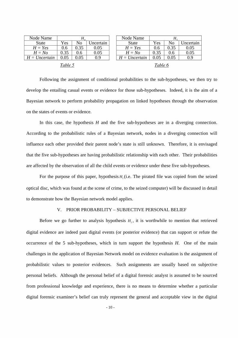
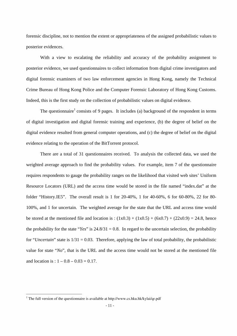
Tables 3 to 6 provide the conditional probabilities of hypotheses 2H to 5H given the state of

hypothesis H.

Node Name 1H State Yes No Uncertain

H = Yes 0.6 0.35 0.05 H = No 0.35 0.6 0.05

H = Uncertain 0.05 0.05 0.9

H = Yes 0.6 0.35 0.05


H = Yes 0.6 0.35 0.05 H = No 0.35 0.6 0.05

H = Uncertain 0.05 0.05 0.9


H = Yes 0.6 0.35 0.05 H = No 0.35 0.6 0.05

H = Uncertain 0.05 0.05 0.9

H

1H 2H 4H 3H 5H

Table 2

Table 3 Table 4

- 10 -

Following the assignment of conditional probabilities to the sub-hypotheses, we then try to

develop the entailing casual events or evidence for those sub-hypotheses. Indeed, it is the aim of a

Bayesian network to perform probability propagation on linked hypotheses through the observation

on the states of events or evidence.

In this case, the hypothesis H and the five sub-hypotheses are in a diverging connection.

According to the probabilistic rules of a Bayesian network, nodes in a diverging connection will

influence each other provided their parent node’s state is still unknown. Therefore, it is envisaged

that the five sub-hypotheses are having probabilistic relationship with each other. Their probabilities

are affected by the observation of all the child events or evidence under these five sub-hypotheses.

For the purpose of this paper, hypothesis 1H (i.e. The pirated file was copied from the seized

optical disc, which was found at the scene of crime, to the seized computer) will be discussed in detail

to demonstrate how the Bayesian network model applies.

V. PRIOR PROBABILITY – SUBJECTIVE PERSONAL BELIEF

Before we go further to analysis hypothesis 1H , it is worthwhile to mention that retrieved

digital evidence are indeed past digital events (or posterior evidence) that can support or refute the

occurrence of the 5 sub-hypotheses, which in turn support the hypothesis H. One of the main

challenges in the application of Bayesian Network model on evidence evaluation is the assignment of

probabilistic values to posterior evidences. Such assignments are usually based on subjective

personal beliefs. Although the personal belief of a digital forensic analyst is assumed to be sourced

from professional knowledge and experience, there is no means to determine whether a particular

digital forensic examiner’s belief can truly represent the general and acceptable view in the digital


H = Yes 0.6 0.35 0.05 H = No 0.35 0.6 0.05

H = Uncertain 0.05 0.05 0.9


H = Yes 0.6 0.35 0.05 H = No 0.35 0.6 0.05

H = Uncertain 0.05 0.05 0.9 Table 5 Table 6

- 11 -

forensic discipline, not to mention the extent or appropriateness of the assigned probabilistic values to

posterior evidences.

With a view to escalating the reliability and accuracy of the probability assignment to

posterior evidence, we used questionnaires to collect information from digital crime investigators and

digital forensic examiners of two law enforcement agencies in Hong Kong, namely the Technical

Crime Bureau of Hong Kong Police and the Computer Forensic Laboratory of Hong Kong Customs.

Indeed, this is the first study on the collection of probabilistic values on digital evidence.

The questionnaire1 consists of 9 pages. It includes (a) background of the respondent in terms

of digital investigation and digital forensic training and experience, (b) the degree of belief on the

digital evidence resulted from general computer operations, and (c) the degree of belief on the digital

evidence relating to the operation of the BitTorrent protocol.

There are a total of 31 questionnaires received. To analysis the collected data, we used the

weighted average approach to find the probability values. For example, item 7 of the questionnaire

requires respondents to gauge the probability ranges on the likelihood that visited web sites’ Uniform

Resource Locators (URL) and the access time would be stored in the file named “index.dat” at the

folder “History.IE5”. The overall result is 1 for 20-40%, 1 for 40-60%, 6 for 60-80%, 22 for 80-

100%, and 1 for uncertain. The weighted average for the state that the URL and access time would

be stored at the mentioned file and location is : (1x0.3) + (1x0.5) + (6x0.7) + (22x0.9) = 24.8, hence

the probability for the state “Yes” is 24.8/31 = 0.8. In regard to the uncertain selection, the probability

for “Uncertain” state is 1/31 = 0.03. Therefore, applying the law of total probability, the probabilistic

value for state “No”, that is the URL and the access time would not be stored at the mentioned file

and location is : 1 – 0.8 – 0.03 = 0.17.

1 The full version of the questionnaire is available at http://www.cs.hku.hk/kylai/qr.pdf

- 12 -

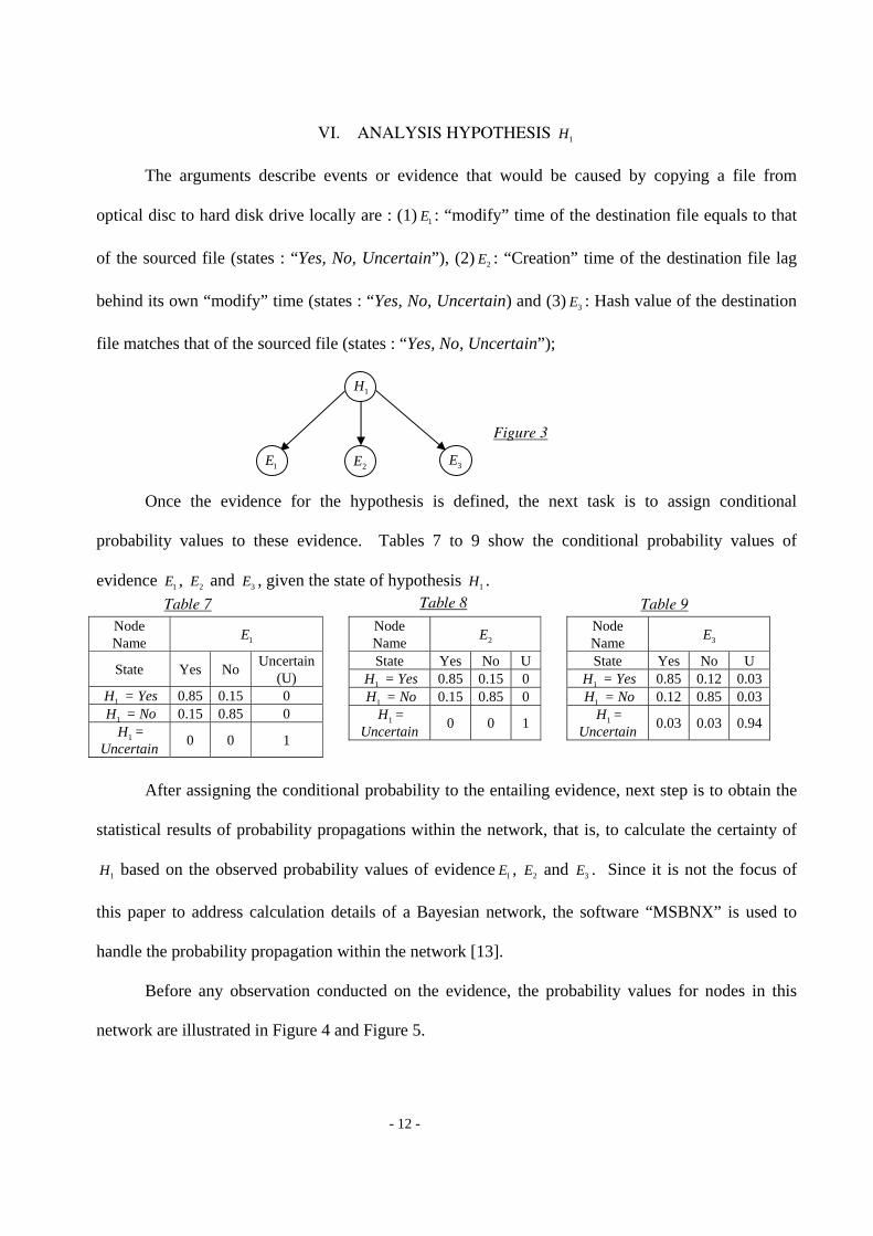
VI. ANALYSIS HYPOTHESIS 1H

The arguments describe events or evidence that would be caused by copying a file from

optical disc to hard disk drive locally are : (1) 1E : “modify” time of the destination file equals to that

of the sourced file (states : “Yes, No, Uncertain”), (2) 2E : “Creation” time of the destination file lag

behind its own “modify” time (states : “Yes, No, Uncertain) and (3) 3E : Hash value of the destination

file matches that of the sourced file (states : “Yes, No, Uncertain”);

Once the evidence for the hypothesis is defined, the next task is to assign conditional

probability values to these evidence. Tables 7 to 9 show the conditional probability values of

evidence 1E , 2E and 3E , given the state of hypothesis 1H .

After assigning the conditional probability to the entailing evidence, next step is to obtain the

statistical results of probability propagations within the network, that is, to calculate the certainty of

1H based on the observed probability values of evidence 1E , 2E and 3E . Since it is not the focus of

this paper to address calculation details of a Bayesian network, the software “MSBNX” is used to

handle the probability propagation within the network [13].

Before any observation conducted on the evidence, the probability values for nodes in this

network are illustrated in Figure 4 and Figure 5.

Node Name 1E

State Yes No Uncertain (U)

1H = Yes 0.85 0.15 0 1H = No 0.15 0.85 0

1H = Uncertain 0 0 1

Node Name 2E

State Yes No U1H = Yes 0.85 0.15 01H = No 0.15 0.85 0

1H = Uncertain 0 0 1

Node Name 3E

State Yes No U 1H = Yes 0.85 0.12 0.031H = No 0.12 0.85 0.03

1H = Uncertain 0.03 0.03 0.94

1H

1E 2E 3E

Table 7 Table 8 Table 9

Figure 3

- 13 -

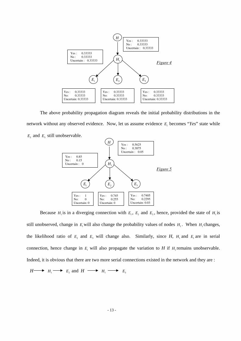
The above probability propagation diagram reveals the initial probability distributions in the

network without any observed evidence. Now, let us assume evidence 1E becomes “Yes” state while

2E and 3E still unobservable.

Because 1H is in a diverging connection with 1E , 2E and 3E , hence, provided the state of 1H is

still unobserved, change in 1E will also change the probability values of nodes 1H . When 1H changes,

the likelihood ratio of 2E and 3E will change also. Similarly, since H, 1H and 1E are in serial

connection, hence change in 1E will also propagate the variation to H if 1H remains unobservable.

Indeed, it is obvious that there are two more serial connections existed in the network and they are :

H 2E and H 1H 3E

1H

1E 2E 3E

H Yes : 0.33333 No : 0.33333 Uncertain : 0.33333

Yes : 0.33333 No : 0.33333 Uncertain : 0.33333

Yes : 0.33333 No: 0.33333 Uncertain: 0.33333

1H

1E 2E 3E


Yes : 0.85 No : 0.15 Uncertain : 0

Yes : 1 No: 0 Uncertain: 0

Yes : 0.745 No: 0.255 Uncertain: 0

Yes : 0.7405 No: 0.2295 Uncertain: 0.03

Yes : 0.33333 No: 0.33333 Uncertain: 0.33333

Yes : 0.33333 No: 0.33333 Uncertain: 0.33333

1H

Figure 4

Figure 5

- 14 -

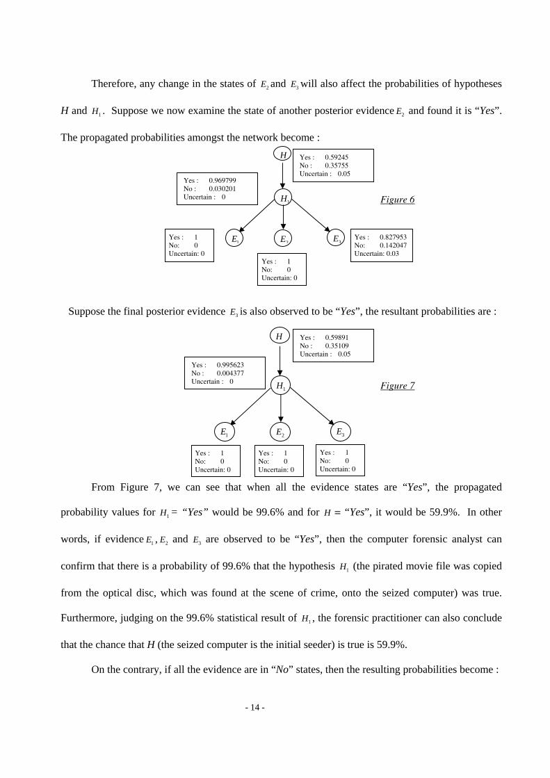
Therefore, any change in the states of 2E and 3E will also affect the probabilities of hypotheses

H and 1H . Suppose we now examine the state of another posterior evidence 2E and found it is “Yes”.

The propagated probabilities amongst the network become :

Suppose the final posterior evidence 3E is also observed to be “Yes”, the resultant probabilities are :

From Figure 7, we can see that when all the evidence states are “Yes”, the propagated

probability values for 1H = “Yes” would be 99.6% and for H = “Yes”, it would be 59.9%. In other

words, if evidence 1E , 2E and 3E are observed to be “Yes”, then the computer forensic analyst can

confirm that there is a probability of 99.6% that the hypothesis 1H (the pirated movie file was copied

from the optical disc, which was found at the scene of crime, onto the seized computer) was true.

Furthermore, judging on the 99.6% statistical result of 1H , the forensic practitioner can also conclude

that the chance that H (the seized computer is the initial seeder) is true is 59.9%.

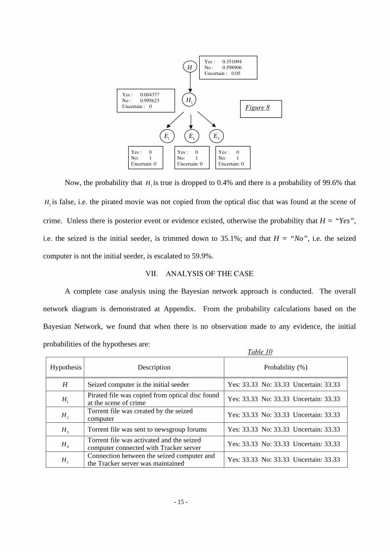
On the contrary, if all the evidence are in “No” states, then the resulting probabilities become :

1H

1E 2E 3E


Yes : 0.969799 No : 0.030201 Uncertain : 0



Yes : 0.827953 No: 0.142047 Uncertain: 0.03

1H

1E 2E 3E


Yes : 0.995623 No : 0.004377 Uncertain : 0




Figure 6

Figure 7

- 15 -

Now, the probability that 1H is true is dropped to 0.4% and there is a probability of 99.6% that

1H is false, i.e. the pirated movie was not copied from the optical disc that was found at the scene of

crime. Unless there is posterior event or evidence existed, otherwise the probability that H = “Yes”,

i.e. the seized is the initial seeder, is trimmed down to 35.1%; and that H = “No”, i.e. the seized

computer is not the initial seeder, is escalated to 59.9%.

VII. ANALYSIS OF THE CASE

A complete case analysis using the Bayesian network approach is conducted. The overall

network diagram is demonstrated at Appendix. From the probability calculations based on the

Bayesian Network, we found that when there is no observation made to any evidence, the initial

probabilities of the hypotheses are:

Hypothesis Description Probability (%)

H Seized computer is the initial seeder Yes: 33.33 No: 33.33 Uncertain: 33.33

1H Pirated file was copied from optical disc found at the scene of crime Yes: 33.33 No: 33.33 Uncertain: 33.33

2H Torrent file was created by the seized computer Yes: 33.33 No: 33.33 Uncertain: 33.33

3H Torrent file was sent to newsgroup forums Yes: 33.33 No: 33.33 Uncertain: 33.33

4H Torrent file was activated and the seized computer connected with Tracker server Yes: 33.33 No: 33.33 Uncertain: 33.33

5H Connection between the seized computer and the Tracker server was maintained Yes: 33.33 No: 33.33 Uncertain: 33.33

1H

1E 2E 3E


Yes : 0.004377 No : 0.995623 Uncertain : 0




Figure 8

Table 10

- 16 -

If we now switch all the entailing evidence to state “Yes” the propagated probability values for

the hypotheses are:

Hypothesis “Yes” (%) “No” (%) “Uncertain” (%) H 92.54 7.45 0.01

1H 99.71 0.29 0 2H 99.98 0.0015 0.0185 3H 99.98 0.02 0 4H 99.93 0.07 0 5H 89.31 10.47 0.22

According to the trial verdict reports, there was no indication that the created torrent file was

found existed in the seized computer. Moreover, there was no mention about the existent of cookies

in the judgment regarding the publishing of the torrent file at newsgroup forums. Therefore we

should amend corresponding observations on the existence of the created Torrent file (node “ E8 ” at

Appendix) and cookies of newsgroup forum (node “ E14 ” at Appendix) from “Yes” to “No” in order to

reveal their impact to the hypotheses.

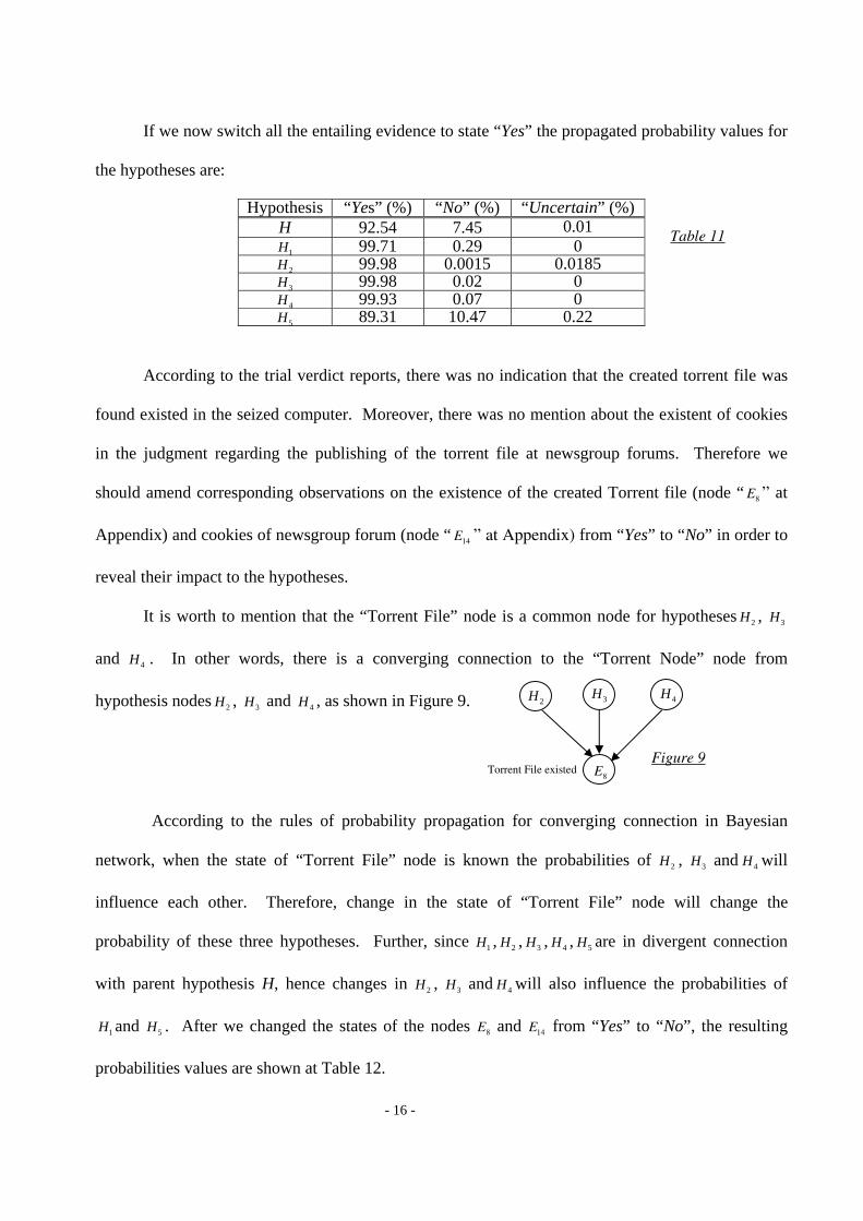
It is worth to mention that the “Torrent File” node is a common node for hypotheses 2H , 3H

and 4H . In other words, there is a converging connection to the “Torrent Node” node from

hypothesis nodes 2H , 3H and 4H , as shown in Figure 9.

According to the rules of probability propagation for converging connection in Bayesian

network, when the state of “Torrent File” node is known the probabilities of 2H , 3H and 4H will

influence each other. Therefore, change in the state of “Torrent File” node will change the

probability of these three hypotheses. Further, since 1H , 2H , 3H , 4H , 5H are in divergent connection

with parent hypothesis H, hence changes in 2H , 3H and 4H will also influence the probabilities of

1H and 5H . After we changed the states of the nodes E8 and E14 from “Yes” to “No”, the resulting

probabilities values are shown at Table 12.

Torrent File existed

2H 3H 4H

E8

Table 11

Figure 9

- 17 -

Hypothesis “Yes” (%)

“No” (%)

“Uncertain” (%)

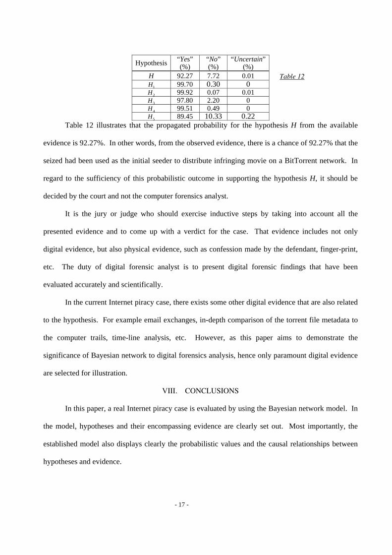
H 92.27 7.72 0.01 1H 99.70 0.30 0 2H 99.92 0.07 0.01 3H 97.80 2.20 0 4H 99.51 0.49 0 5H 89.45 10.33 0.22

Table 12 illustrates that the propagated probability for the hypothesis H from the available

evidence is 92.27%. In other words, from the observed evidence, there is a chance of 92.27% that the

seized had been used as the initial seeder to distribute infringing movie on a BitTorrent network. In

regard to the sufficiency of this probabilistic outcome in supporting the hypothesis H, it should be

decided by the court and not the computer forensics analyst.

It is the jury or judge who should exercise inductive steps by taking into account all the

presented evidence and to come up with a verdict for the case. That evidence includes not only

digital evidence, but also physical evidence, such as confession made by the defendant, finger-print,

etc. The duty of digital forensic analyst is to present digital forensic findings that have been

evaluated accurately and scientifically.

In the current Internet piracy case, there exists some other digital evidence that are also related

to the hypothesis. For example email exchanges, in-depth comparison of the torrent file metadata to

the computer trails, time-line analysis, etc. However, as this paper aims to demonstrate the

significance of Bayesian network to digital forensics analysis, hence only paramount digital evidence

are selected for illustration.

VIII. CONCLUSIONS

In this paper, a real Internet piracy case is evaluated by using the Bayesian network model. In

the model, hypotheses and their encompassing evidence are clearly set out. Most importantly, the

established model also displays clearly the probabilistic values and the causal relationships between

hypotheses and evidence.

Table 12

- 18 -

Through the evaluation on prior evidence and the probabilistic analysis on posterior evidence,

the Bayesian network model is able to help computer forensics analyst to assess possible states of

each piece of evidence. In addition, the model can determine the evidence that will have the most

effect on the forensics findings. It can also illustrate how digital evidence affects each other and the

relating hypotheses. Thus, the Bayesian model is not only an analytical tool used in evidence

evaluation, but also a tracking tool to enable other forensics practitioners to review and to re-examine

the original forensics findings.

Perhaps the most significant contribution of the model is that it can offer a way to handle

evidence that are of uncertainty or unobserved status. Most of time, it is difficult to retrieve all

possible evidence of a case, or that the collected evidence are contradictory to the hypotheses.

Sometimes, forensic analyst may tend to ignore evidence that are uncertain or contradict to the

formulated hypotheses, in particular when large amount of digital evidence is involved.

Even if the analyst is cautious and wants to evaluate the impact of uncertain or contradictory

evidence, it is difficult for him to project such influences by simply using his personal intuition.

Furthermore, the analyst is also difficult to crystallize the interactive influences between each piece of

evidence and the relating hypotheses. Obviously, the Bayesian network model is an optimum

solution to solve the problems.

In order to minimize the impact of subjectivity when assigning prior probabilities to the

posterior evidence involved in the BitTorrent case, we have gathered data on probability values

through survey research by administering questionnaires to law enforcement officers who are

involving in computer crime investigation or computer forensic examination. However, the

subjectivity constraints on the sub-hypotheses still prevail. The limitation focuses on the prior

probability assignments to the constructed sub-hypotheses that give rise to the root hypothesis. Since

sub-hypotheses are causal events to digital evidence, hence they are based on the propagation of

probability values of the evidence. It is therefore difficult to ask respondents to evaluate the posterior

- 19 -

probabilistic values of sub-hypotheses unless the posterior beliefs on finite digital evidence can be

established in the first place. Therefore, it is the view of this paper that such limitation deserves

further research and verification by methodology like sensitive analysis such that the reliability,

accuracy, and precision of the Bayesian Network model can be evaluated.

In fact, a Bayesian network model is not focused to give strict answers. The model aims to

develop a traceable and scientific infrastructure that can project the likelihood of a hypothesis. In

order to increase the accuracy of the projection or to simplify the Bayesian construction cycle, there

are various approaches and methodologies developed. For example, the Markov property is

developed to handle the computational problem when there are large common nodes or large joint

probability propagation occurred in a Bayesian network. By Learning methods, such as structural

learning, parametric learning, adaptation learning, etc., we can use experience gained from these

models to construct an accurate Bayesian network and to assign sensible probability values to

evidence.

This paper has demonstrated the potentials of applying the Bayesian Network model in

computer forensics analyses. Since computer forensics science is still in its developing stage, a

Bayesian Network model analysis can offer scientific grounds for a computer forensics practitioner to

evaluate and to justify his forensics findings. Moreover, further research and analysis are needed to

enhance the inference capability and accuracy of the Bayesian Network model before it can widely be

adopted in the computer forensics discipline.

REFERENCES

[1] P. Good, ‘Applying Statistics in the Courtroom: A New Approach for Attorneys and Expert Witnesses’, Florida: CRC Press LLC, 2001.

[2] R. Cook, I. Evett, G. Jackson, P. Jones and J. Lambert, ‘A model for case assessment and

interpretation’, Science and Justics, 38:151-156, 1998. [3] R. Loui, J. Norman, J. Alpeter, D. Pinkard, D. Craven, J. Linsday and M. Foltz, ‘Progress on

room 5: a testbed for public interactive semi-formal legal argumentation’, Proceeding of the 6th International Conference on Artificial Intelligence and Law, pp 207-214, 1997.

- 20 -

[4] D. Walton, ‘Argumentation and theory of evidence’, New Trends in Criminal Investigation and Evidence, 2:711-732, 2000.

[5] J. Mortera, A. Dawid and S. Layritzen, ‘Probabilistic expert systems for DNA mixture profiling’,

Theoretical Population Biology, 63(3):191-205, 2003. [6] H. Prakken, C. Reed and D. Walton, ‘Argumentation schemes and generalizations in reasoning

about evidence’, Proceeding of the 9th International Conference on Artificial Intelligence and Law, 2003.

[7] CGG Aitken, F. Taroni, ‘Statistics and the Evaluation of Evidence for Forensic Scientists’, New

York: John Wiley & Sons, 2004. [8] J. Jones, Y. Xiang and S. Joseph, ‘Bayesian Probabilistic Reasoning in Design’, IEEE Pac

Rim ’93, pp 501-504. [9] R. Cowell, ‘Introduction to inference for Bayesian networks’, Learning in Graphical Models, pp

9-26, Cambridge: MIT Press, 1999. [10] J. Pearl, ‘Probabilistic Reasoning in Intelligent Systems: Networks of Plausible Inference’. [11] J. Keppens and J. Zeleznikow, ‘A model based reasoning approach for generating plausible

crime scenarios from evidence’, Proceeding of the 9th International Conference on Artificial Intelligence and Law, pp 51-59, 2003.

[12] D. Poole, ‘Probabilistic Horn adduction and Bayesian networks’, Artificial Intelligence,

6491):81-129, 1993. [13] “Bayesian Network Editor and Tool Kit” http://research.microsoft.com/adapt/MSBNx (accessed on 12 February 2007). [14] International Organization on Computer Evidence, ‘International principles for computer

evidence’, Forensic Science Communications, 2(2), April 2000. [15] the International Association of Computer Investigative Specialist, ‘Forensic procedures’,

http://www.iacis.com/iacisv2/pages/forensicprocedures.php (accessed on 14 February 2007). [16] T. Grance, S. Chevalier, K. Kent and H. Dang, ‘Guide to computer and network data analysis:

Applying forensic techniques to incident response’, National Institute of Standards and Technology, Special Pub. 800-86.

[17] S. Ciardhuáin, ‘An extended model of cyber investigation’, International Journal of Digital

Evidence, Volume 3, Issue 1, Summer 2004. [18] S. Peisert, M. Bishop, S. Karin, and K. Marzullo, “Principles-Driven Forensic Analysis,”

Proceedings of the 2005 New Security Paradigms Workshop pp. 85–93 (Sep. 2005). [19] F. Tushabe, ‘The enhanced digital investigation process model’, Digital Forensic Research

Workshop, 2004. [20] ‘HKSAR v Chan Nai Ming TMCC 1268/2005’,

http://www.hklii.org/cgi-hklii/disp.pl/hk/jud/en/hksc/2005/TMCC001268A%5f2005.html (accessed on 14 February 2007).

[21] F. Jensen, ‘An introduction to Bayesian network’, London: UCL Press, 1995.

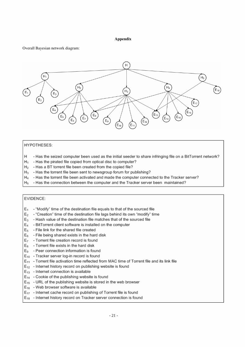
- 21 -

Appendix Overall Bayesian network diagram:

Documents

Computer Forensics using Bayesian Network: A Case Studyi.cs.hku.hk/~cisc/forensics/papers/BayesianNetwork.pdf · - 2 - I. INTRODUCTION The proliferation of computer crimes has driven