Computer Exercises1. Generate a stationary process AR(2) denoted by . Suppose that

Here, the parameters of are determined by yourselves. Then generate a

white noise with the variance . The received signal is

with a variable SNR. Put the received the signal to a Wiener-filter, the length of

the filter is N. And the output is denoted by .

① Study on the relationship between the cost function and SNR of the signal,

provided the length of the Wiener-filter is given.

② Study on the relationship between the cost function and length of the filter,

provided the SNR is given.

.③ When one-step prediction is done, how about the cost function varies with the

SNR and length of the Wiener-filter.

2. Examine the transient behavior of the steepest-descent algorithm applied to a

predictor that operates on a real-valued autoregressive (AR) process. Fig. P2

shows the structure of the predictor, assumed to contain two tap weights that

denoted by and ; the dependence of these tap weights on the number

of iterations, n, emphasizes the transient condition of the predictor. The AR

process is described by the second-order difference equation

where the sample is drawn from a white-noise process of zero mean and

variance . The AR parameters and are chosen so that the roots of the

characteristic equation

are complex; that is, . The particular values assigned to and are

determined by the desired eigenvalue spread . For specified values of and

, the variance of of the white-noise is chosen to make the process

have variance .

The requirement is to evaluate the transient behavior of the steepest-decent

algorithm for the following conditions:

Varying eigenvalue spread and fixed step-size parameter

Varying step-size parameter and fixed eigenvalue spread

Plot the learning curve please.

3. By adaptive filtering, do the research work on the picking up of a signal with only one frequency.

① Suppose that ,here is a wideband signal, f is arbitrary chosen, you are required to extract .

② Suppose that , is a wideband

signal, can be selected arbitrary. You are required:

To extract both of the two signals with single frequency; Suppose , extract the , do the research work on

the effect that SNR (Signal-Noise Ratio), . Here N is the

length of the data.

4. For this computer experiment involving the LMS algorithm, use a first-order,

autoregressive (AR) process to study the effects of ensemble averaging on the

transient characteristics of the LMS algorithm for real data.

Consider an AR process of order one, described by the difference equation

where is the (one and only) parameter of the process and is a zero-mean

white-noise process of variance . To estimate the parameter , use an adaptive

predictor of order one, as depicted in Fig. P4.

Given different sets of AR parameters, fixed the step-size parameter, and the

initial condition .

Please plot the transient behavior of weight including the single

realization and ensemble-averaged result.

The transient behavior of the squared prediction error

Draw the experimental learning curves , what is the result when the step-

size parameter is reduced.

5. Study the use of the LMS algorithm for adaptive equalization of a linear dispersive

channel that produces (unknown) distortion. Assume that the data are all real

valued. Fig. P5 shows the block diagram of the system used to carry out the study.

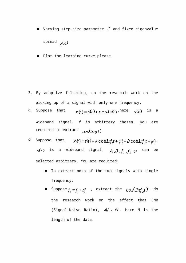
Random-number generator 1 provides the test signal , used for probing the

channel, whereas random-number generator 2 serves as the source of additive

white noise that corrupts the channel output. These two random-number

generators are independent of each other. The adaptive equalizer has the task of

correcting for the distortion produced by the channel in the presence of the

additive noise. Random-number generator 1, after suitable delay, also supplies the

desired response applied to the adaptive equalizer in the form of the training

sequence.

The experiment is required

To evaluate the response of the adaptive equalizer using the LMS algorithm

to changes in the eigenvalue spread and step-size parameter .

The effect on the squared error when length of the delay and the length of the

data is changed.

6. Generate 100 samples of a zero-mean white noise sequence with variance

, by using a uniform random number generator.

(a) Compute the autocorrelation of for .(b) Compute the periodogram estimate and plot it.

(c) Generate 10 different realizations of , and compute the corresponding

sample autocorrelation sequences , and . Compute

the average autocorrelation sequence as and the

corresponding periodogram for .

(d) Compute and plot the average periodogram using the Bartlet method.

(e) Compute on the results in parts (a) through (d).

7. A random signal is generated by passing zero-mean white Gaussian noise with

(a) Sketch a typical plot of the theoretical power spectrum for a small value

of the parameter a (i.e., 0<a<0.1). Pay careful attention to the value of the two spectral peaks and the value of for .

(b) Let a=0.1. Determine the section length M required to resolve the spectral

peaks of when using Bartlett’s method.

(c) Consider the Blackman-Turkey method of smoothing the periodogram. How

many lags of the correlation estimate must be used to obtain resolution

comparable to that of the Bartlett estimate considered in part (b)? How many

data must be used if the variance of the estimate is to be comparable to that of a

four-section Bartlett estimate?

(d) Generate a data sequence x(n) by passing white Gaussian noise through H(z)

and compute the spectral estimates based on the Bartlett and Blackman-Tukey

methods and, thus, confirm the results obtained in parts (b) and (c).

(e) For a=0.05, fit an AR(4) model to 100 samples of the data based on the Yule-

Walker method, and plot the power spectrum. Avoid transient effects by

discarding the first 200 samples of the data.

(f) Repeat part (e) with the Burg method.

(g) Repeat parts (e) and (f) for 50 data samples, and comment on similarities and

differences in the results.

8. Research on the performance of AR power spectrum estimates that were obtained

with artificially generated data. The objective is to compare the spectral estimation

methods on the basis of their frequency resolution, bias and robustness in the

presence of additive noise.The data consist of either one or two sinusoids and

additive Gaussian noise. The two sinousoids are space apart. The underlying

process is ARMA(p,q), p and q are decided by yourself.

Estimate the PSD by Yule-Walker method, research on the effects varying

data length, SNR, the order of AR model.

Estimate the PSD by Burg method, research on the effects varying data

length, SNR, the order of AR model.

Estimate the PSD by LS method, research on the effects varying data

length, SNR, the order of AR model.

9．Consider the adaptive predictor shown in Fig. P9

Fig. P9

(a) Determine the quadratic performance index and the optimum parameters for the

signal

where is white noise with variance

(b) Generate a sequence of 1000 samples of , and use the LMS algorithm to

adaptively obtain the predictor coefficients. Compare the experimental results

with the theoretical values obtained in part (a). Use a step size of .

(c) Repeat the experiment in part (b) for trials with different noise sequences,

and compute the average values of the predictor coefficients. Comment on how

these results compare with the theoretical values in part (a).

10. An autoregressive process is described by the difference equation

(a) Generate a sequence of N=1000 samples of , where is a white noise

sequence with variance . Use the LMS algorithm to determine the

parameters of a second-order ( ) linear predictor. Begin with

. Plot the coefficients and as a function of the

iteration number.

(b) Repeat part (a) for 10 trials, using different noise sequences, and superimpose

the 10 plots of and .

(c) Plot the learning curve for the average (over the 10 trials) MSE for the data in

part (b).

11. A random process is given as

,

where is an additive white noise sequence with variance

(a) Generate N=1000 samples of and simulate an adaptive line enhancer of

length . Use the LMS algorithm to adapt the ALE.

(b) Plot the output of the ALE.

(c) Compute the autocorrelation of the sequence .

(d) Determine the theoretical values of the ALE coefficients and compare them

with the experimental values.

(e) Compute and plot the frequency response of the linear predictor (ALE).

(f) Compute and plot the frequency of the prediction-error filter.

(g) Compute and plot the experimental values of the autocorrelations of the

output error sequence for .

(h) Repeat the experiment for 10 trials, using different noise sequences, and

superimpose the frequency response plots on the same graph.

(i) Comment on the result in parts (a) through (h).

12. Consider an AR process defined by the difference equation

where is an additive white noise of zero mean and variance . The AR

parameters and are both real valued: ,

(a) Calculate the noise variance such that the AR process has unit

variance. Hence generate different realizations of the process .

(b) Given the input , an LMS filter of length is used to estimate the

unknown AR parameters and . The step-size parameter is assigned the

value 0.05. Justify the use of this design value in the application of the small-

step-size theory.

(c) For one realization of the LMS filter, compute the prediction error

and the two tap-weight errors

and

Using power spectral plots of and , show that behaves

as white noise, whereas and behave as low-pass processes.

(d) Compute the ensemble-average learning curve of the LMS filter by averaging

the squared value of the prediction error over an ensemble of 100

different realizations of the filter.

(e) Using the small-step-size statistical theory, compute the theoretical learning

curve of the LMS filter and compare your result against the measured result of

part (d).

13. Consider a linear communication channel whose transfer function may take one of

three possible forms:

(i)

(ii)

(iii)

The channel output, in response to the input , is defined by

where is the impulse response of the channel and is additive white

Gaussian noise with zero mean and variance . The channel input

consists of a Bernoulli sequence with .

The purpose of the experiment is to design an adaptive equalizer trained by

using the LMS algorithm with step-size parameter . In structural

terms, the equalizer is built around a transversal filter with 21 taps. For desired

response, a delayed version of the channel input, namely , is supplied to

the equalizer. For each of the possible transfer functions listed under (i), (ii) and

(iii) do the following:

(a) Determine the optimum value of the delay that minimizes the mean-square

error at the equalizer output.

(b) For the optimum delay determined in part (a), plot the learning curve of the

equalizer by averaging the squared value of the error signal over an ensemble

of 100 independent trials of the experiment.

14．To illustrate the optimum filtering theory developed in the preceding sections,

consider a regression model of order with its parameter vector denoted by

The statistical characterization of the model, to be real valued, as follows:

.① The correlation matrix of the input vector is

where the dashed lines are included to identify the submatrices that

correspond to vary filter lengths.

.② The cross-correlation vector between the input vector and observable

data is

where the value of the fourth entry ensures that the model parameter is

zero.

.③ The variance of observable data is

.④ The variance of the additive white noise is

The requirement is to do three things:

· Investigate the variation of the minimum mean-square error produced by

a Wiener filter of varying length

· Display the error-performance surface of a Wiener filter with length .

· Compute the canonical form of the error-performance surface.