COMPUTER CORNER EDITOR DePaul · PDF fileCOMPUTER CORNER EDITOR Richard Johnsonbaugh ... the same radius as the ball, then it will not be distorted when the leather is stretched to

COMPUTER

CORNER

EDITOR

Richard Johnsonbaugh School of Computer Science, Telecommunications and Information Systems DePaul University Chicago, IL 60604-2302

johnsonbaugh @ cs. depaul. edu

In this column, readers are encouraged to share their expertise and experiences with computer tech?

nology as it relates to college mathematics. Articles illustrating how computers can enhance pedagogy, solve mathematics problems, and model real-life situations are especially welcome.

Classroom Computer Capsules feature new examples of using the computer to enhance teach?

ing. These short articles demonstrate the use of readily available computing resources to present or elucidate familiar topics in ways that can have an immediate and beneficial effect in the classroom.

Send submissions for both columns to Richard Johnsonbaugh.

Designing a Baseball Cover

Richard B. Thompson

Richard Thompson ([email protected]) earned a Ph.D. in algebraic topoiogy from the University of Wisconsin and

has taught at the University of Arizona since 1967. Besides

topological research, implementing an individualized instruc- tion program in algebra, and curriculum development in

mathematics and statistics courses, his interests include

using computers effectively in undergraduate courses. Away from academia he enjoys ski mountaineering and sailing.

Problems in design, even those of a rather frivolous nature, can produce some very

interesting mathematics. Consider the 130-year-old problem of designing the cover

for a baseball. Early experimental work on this problem involved the freehand draw?

ing of plane figures. We will use geometric insight and calculus to give a relatively

easy solution of the problem in space. Next, a differential equation will be derived

that gives a mathematical solution with plane figures, in the style of the early efforts.

Finally, we will see how well trial and error have worked, by looking at the cover

design that is currently used in the manufacture of major league baseballs.

The Problem

In the 1860s C. H. Jackson patented a pen and ink drawing of a plane shape that

could be used to form the cover of a baseball. This shape is still in use today on all

major league baseballs. According to Bill Deane, a Senior Research Associate with

the Baseball Hall of Fame, Mr. Jackson's design was produced by "trial and error."

In practical terms, he wanted a piece of leather that could be sewn to an identical

piece and then stretched to cover the yarn-wound core of a ball.

48 THE COLLEGE MATHEMATICS JOURNAL

Figure 1. Left, Jackson's cover pattern. Right, two flats ready for stitching.

We will refer to each pattern piece (Figure 1, left) as aflat. Two flats, ready for

stitching, are shown in Figure 1 on the right. The stitched pair of flats, shown in

Figure 2 (left), will be called a preball. If the seam of the preball lies on a sphere of

the same radius as the ball, then it will not be distorted when the leather is stretched

to form a ball, as shown on the right in Figure 2. A preball whose seam fits on the

surface of a sphere will be called acceptable; its associated flat is also acceptable. Mr. Jackson tried to draw an acceptable flat that satisfied several design constraints.

Baseballs were expected to have the nominal circumference of 9| inches and two

parts of the seam were to be located in such a way as to provide a good grip for the

pitcher's fingers. Measurements of current balls indicate that this distance (the are

length S in Figure 2) is 1 ~ inches. Apparently, Mr. Jackson also wanted a flat that

was symmetrical about both its horizontal and vertical axes. The difficulty of getting close to an acceptable flat that met these criteria must have required many trials, and

a lot of errors!

Recently, physicists have attempted to find practical considerations that determine

a unique shape for the flats in a baseball cover [1], [2]. We take a different point of

view, and show that acceptable flats are far from unique. In fact, we have consider-

able freedom in designing them.

Figure 2. Left, preball. Right, its radial expansion.

VOL. 29, NO. 1, JANUARY 1998 49

From a mathematical point of view, it is helpful to focus our attention on the seam

of the preball. A flat is acceptable if the resulting seam is a simple closed curve on

a sphere, that is the common boundary of two congruent regions. This requirement could be met by a flat with the shape of a disk of suitable radius; the resulting seam would then be a great circle on the finished ball. (In fact, such covers were

actually designed and used, under the name of "belt balls.") In addition to placing

great demands on the stretchability of the leather, such a design does not meet

the pitcher's requirement for close sections of the seam for a good grip. This latter

requirement can be obtained by distorting the great circle seam. It is clear that there

is nothing unique about the shape of the seam. In most of our figures and design

work, we will avoid excessive creativity and display only shapes that resemble the

ball of Mr. Jackson's construction.

There are two ways to design a baseball cover:

1. Draw a flat in the plane and then wrap two copies of this around the ball.

2. Find a parametrization ofthe seam on the ball, and then unwrap the two resulting regions to form flats.

Mr. Jackson chose the first option, since it is simpler and is the only practical plan for pen and ink experimentation. The main difficulty of drawing flats in the plane is

that it appears to be necessaiy to specify one-fourth of the entire outline of the flat.

This corresponds to one-fourth of the seam on the preball. It is not at all clear how

to plan ahead so that the seam will lie on the surface of a sphere. The second plan removes this difficulty, since we design directly on a sphere. However, this presents the problem of drawing a seam that separates the sphere into two congruent regions. We will solve this problem by using symmetries in three-space to show that we need

only specify one-eighth of the entire seam. Mathematical analysis and computational

power, by eliminating trial and error, make the apparently more complicated second

plan the better alternative.

Designing on the Ball

We picture the ball as centered at the origin in M3 (Figure 2), with projections onto

the xy-plane and xz-plane as shown in Figures 3a and 3b. In Figure 3a the positive z-axis is pointed from the page toward us, and we consider the part of the seam

that has nonnegative z-coordinates. In Figure 3b the positive y-2ods points from the

page toward us. The circumference is Cn = 9| inches, which determines the radius

R = Co/(27r). We let S = 1-^ inches be the length of the minimum are between two

parts of the seam. Let A be the point on the seam in Figure 3a that has a maximal

x-coordinate. If A = (xn, 2/o> 0), then it is easy to see that

Xo = jRcos(^)'

yo = Rsin{^R

Let B be the point on the seam that projects onto the positive ?/-axis in Fig? ure 3a and onto the positive z-axis in Figure 3b. Its y- and z-coordinates have a

common value, which we will denote by 6n- Since B is on the sphere, we have

Y^O2 + b\ + b\ = R, so 6o = R/V2. Let C be the point in Figure 3a where the

projection of the seam crosses the x-axis. Since flats F\ and F2 are congruent, the

coordinates of point C are (?xn, 0? 2/o)-


*- X

Figure 3. Views from the z-axis (left) and y-axis (right).

Let / : [?xo,xo] ?? M be the function whose graph is the top half of the pro-

jected seam in Figure 3a, and let g and h be the restrictions of / to the left and

right halves of its domain, respectively. Due to the congruence of the seam curves

in Figures 3a and 3b, a point on the seam that projects onto the graph of g has

coordinates (x,g(x),h(?x)). Since the seam lies on the surface of the ball, g(x) =

\/R2 ? x2 ?

h{?x)2. Hence, h : [0,xq] ?> M completely determines /:

m \ fy/& h{-xf

\h{x)

if ? Xq < X < 0,

if 0 < X < Xq. (1)

The x- and ^/-coordinates (x, f(x)) for the projection of a point on the seam deter?

mine the z-coordinate z = ^/R2 ? x2 ?

f(x)2 of the point. Hence, we can use t = x

to parametrize that part of the seam that projects onto the graph of f:

x(t)=t, y(t) = f(t), z(t) = ^R2-t2-f(t)2, fov-xo<t<x0. (2)

Having parametrized one-fourth of the seam, we can splice together copies of

our functions and parametrize the entire seam with t running from 0 to 8#o- To

parametrize the seam, we need only define h : [0,xo] ?> M such that h(0) = 6o and h(xo) = yo- in this matter we have great freedom. As long as h is reasonably well behaved (say, continuously differentiable) and has a graph that stays in the first

quadrant of the projected circle in Figure 3a, there is no mathematical necessity for the selection of any particular function. Our choice must rest upon our mental

picture of a baseball seam.

The best measure of our success is to look at pictures and see if we have something close to the desired appearance of a baseball. To do this, we will select a trial formula

for h and then use it to parametrize a seam.

Our initial choice for h is dictated by two considerations. First, examination of

an actual baseball indicates that the graph of h is relatively straight. Second, math?

ematicians like linearity! We define h to be the linear function, connecting the two

designated points:

h(x) =-x - x0

?6o.

VOL. 29, NO. 1, JANUARY 1998 51

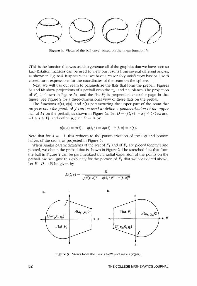
Figure 4. Views of the ball cover based on the linear function h.

(This is the function that was used to generate all of the graphics that we have seen so

far.) Rotation matrices can be used to view our results from several different angles, as shown in Figure 4. It appears that we have a reasonably satisfactory baseball, with

closed form expressions for the coordinates of the seam on the sphere. Next, we will use our seam to parametrize the flats that form the preball. Figures

5a and 5b show projections of a preball onto the xy- and xz- planes. The projection of i7! is shown in Figure 5a, and the flat F2 is perpendicular to the page in that

figure. See Figure 2 for a three-dimensional view of these flats on the preball. The functions x(f),y{t), and z{t) parametrizing the upper part of the seam that

projects onto the graph of f can be used to define a parametrization of the upper half of Fi on the preball, as shown in Figure 5a. Let D = {(?, s) \

? xq < t < xq and ? 1 < s < 1}, and define p, g, r : D ?> R by

p(t, s) = x(t), q(t, s) = sy(t) r(t, s) = z(t).

Note that for s = ?1, this reduces to the parametrization of the top and bottom

halves of the seam, as projected in Figure 5a.

When similar parametrizations of the rest of Fi and of F2 are pieced together and

plotted, we obtain the preball that is shown in Figure 2. The stretched flats that form

the ball in Figure 2 can be parametrized by a radial expansion of the points on the

preball. We will give this explicitly for the portion of F\ that we considered above.

Let E : D ?> R be given by

E(t,s) R

^/p(t,s)2 + q(t,s)2 + r(t,s)2'

Figure 5. Views from the z-axis (left) and y-axis (right).


Multiplying a point (p(t, s), q(t, s),r(t, 5)) on the preball's surface by E(t,s) will

move this point radially outward to the surface of the ball. We can use this to give

parametric equations P, Q, R : D ?> R for the part of the ball that is covered by the

stretched top half of F\. Thus,

P(t, s) = E(t, s)p(t, s) Q(t, s) = E(t, s)q(t, s) R(t, s) = E(t, s)r(t, s).

Since the seam is on the surface of the ball (for s = ?1, p(t, s)2 + q(t, s)2 + r(t, s)2 =

R2), it does not move under the expansion.

Drawing the Flat

We now complete our design task by opening the seam and mathematically "un-

wrapping" flat F\ from the preball to get a plane pattern for a flat.

Referring to Figure 5a, let Ln be the length of the graph of / over [?xn, xn], and

let L : [?xn, xn] ?> [0, Ln] be the are length function for that graph:

L(t) = j ^/l + f'(x)2dx.

I ?Xn

Note that the graph of / has a vertical tangent at (?xq, 0). Hence, L is given by an

improper integral. We will assume that the function h has been chosen so that this

integral converges, and the graph of / has finite length. This is certainly the case for

the linear h that we have used in our examples. Since L is an increasing function, it has an inverse L-1 : [0, Ln] ?> [?xn,xn]. The

center line of Fi projects directly onto the copy of the graph of / in Figure 5b. We

use this to define F : [0, L0] ?> R by F(u) = /(

- L-1(w)). Note that L-1(w) moves

from left to right in Figure 5a, while ? L~l(u) moves from right to left. Figure 6

shows how the graph of F is related to that of /.

U\u) x0

(-L-\u),f(-L-\u)))

Figure 6. Unwrapping a flat.

VOL. 29, NO. 1, JANUARY 1998 53

The plane region V, bounded by the graph of F, the u-axis, and the line u = 0, is

a pattern for the top half of the part of F\ shown in Figure 5a. The region V based

on a linear function h is shown at the bottom of Figure 6. The function <? : V ?> F\

given by

$ (u,v)^(-L-\u),vj(L-\u)))

embeds V into the preball.

Using symmetiy, we can assemble four copies of V to form an acceptable flat. The

resulting shape is that shown on the left in Figure 1. This completes our solution of

the original design problem. We have made a pattern that could be used to cut pieces of leather to form a baseball cover. Note that we have created a parametrization of

the seam, in closed form. Our parametrization of the acceptable flat uses are length and an inverse function, which are computable to any desired accuracy but cannot

be given in closed form.

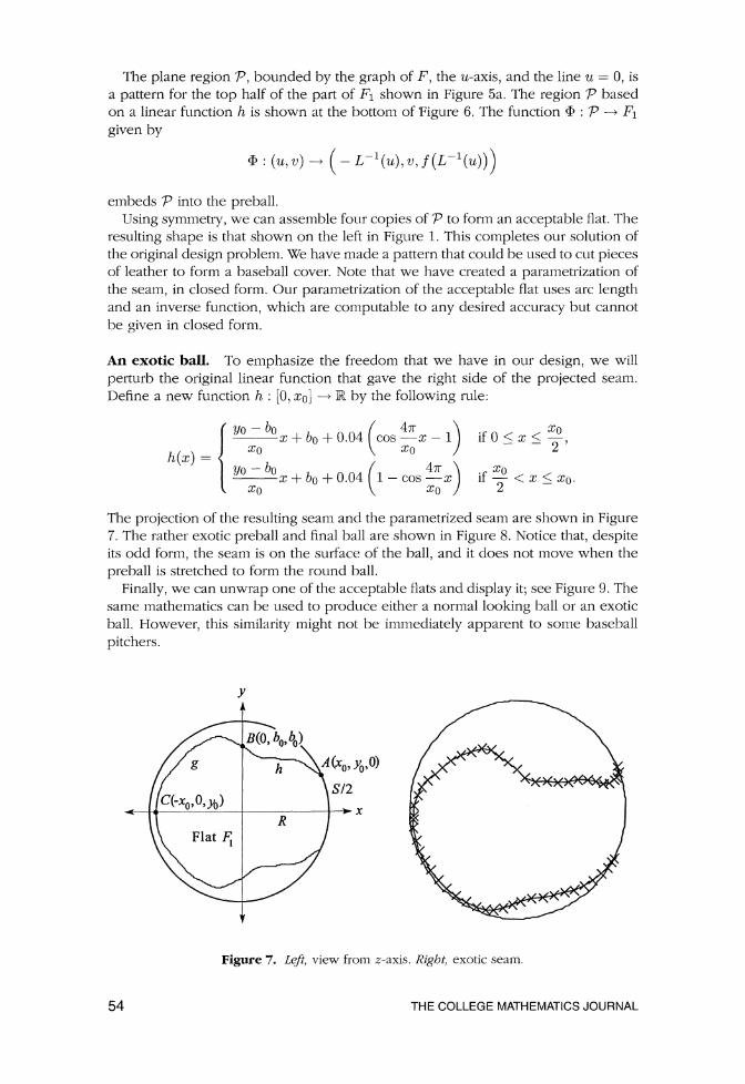
An exotic ball. To emphasize the freedom that we have in our design, we will

perturb the original linear function that gave the right side of the projected seam.

Define a new function h : [0, xq] ?? R by the following rule:

h{x)

-x + b0 + 0.04 cos ?x -1 if 0 < x < -?, x0 \ x0 J 2

y^hx + b0 + 0m(l-cos-x] if^<x<x0. X0 \ X0 J 2

The projection of the resulting seam and the parametrized seam are shown in Figure 7. The rather exotic preball and final ball are shown in Figure 8. Notice that, despite its odd form, the seam is on the surface of the ball, and it does not move when the

preball is stretched to form the round ball.

Finally, we can unwrap one of the acceptable flats and display it; see Figure 9. The

same mathematics can be used to produce either a normal looking ball or an exotic

ball. However, this similarity might not be immediately apparent to some baseball

pitchers.

Figure 7. Left, view from z-axis. Right, exotic seam.


Figure 8. Left, exotic preball. Right, exotic ball.

Figure 9- Exotic flat.

Designing in the Plane

We have used mathematics and computation to design an acceptable flat. Our plan relied heavily on the symmetries of the seam in three dimensions. Is it possible to

realize Mr. Jackson's original goal of designing an acceptable flat in the plane? The

answer is yes. However, we have to work with more complicated mathematics and

be rather clever when we design in the two-dimensional venue.

Since the seam on the ball is determined by one-eighth of its length, we can only

expect to specify one-eighth of the edge of an acceptable flat. To do this, we will

start with a function, F, whose graph forms part of the top boundary of a flat. The

graph of this function will be mathematically wrapped onto the ball as a seam, so

that it projects onto the graph of a function, h, as in Figure 3a. Symmetry determines

the portion of the seam that projects onto the graph of the associated function g. With the seam parametrized over the graph of / in Figure 5a, we will use are length to unwrap the top of the resulting acceptable flat. The top edge of this flat will

extend the graph of the function F. Although the plan is rather straightforward, its

execution requires some real effort.

Suppose that the graph of F : [0, uq] ?> R is part of the edge of a flat , drawn in

a wv-plane, as in Figure 10 (page 56). For the moment, uq will be considered as a

variable. We want to wrap this edge onto the preball in Figure 3a so that it is above

the x?/-plane and projects onto h. Since the wrapped graph of F is to project onto

the entire graph of h, we require that F(0) = yo and F(uo) = &o- There is no way to determine the value of uq before the flat is put into the preball. Hence, uq is left

as a variable.

VOL. 29, NO. 1, JANUARY 1998 55

("oA)

Graph of F

-?-? u

Figure 10. Starting a flat.

We define an are length function K : [0, uq) ?> R along the graph of F,

s = K(u)= [ y/l + F'(w)2dw, Jo

and let s0 = K(u0). This gives K~l : [0, s0] ?> [0, uo]. Now define three-dimensional parametric functions, x,y,z : [0, sq] -> ^> that place

the graph of F onto the surface of the preball as the upper edge of flat F\, as shown

in Figure 3a. As the parameter s runs from 0 to so, the point {x(s),y(s),z(s)) is to

run from right to left along the seam.

It is natural to define y by y(s) = F(kK~1(s)). If x and y are determined, we can

use the fact that the image must lie on the ball to define z(s) = ^/R2 ?

x(s)2 ?

y(s)2. The definition of x requires more careful thought. We want to preserve are length, as the edge of the flat is mapped onto the seam of the preball. Hence, the are

length along the seam from (#(0),2/(0), 2(0)) to (x(s),y{s),z{s)) must be s for all

se [o,80]:

/ y/x'(<r)2 + y'(a)2 + z'(a)2 da. Jo

(3)

Differentiating both sides of equation (3) with respect to s, and then squaring both

sides of the resulting equation, yields

l = x'{s)2 + y\s)2 + zl{s)2.

The derivatives of y and z can be computed from previous formulas.

y'{s) = F'{K-\s)){K-l)'{s),

z, = x(s)x'{s)+y(s)y'(s)

^/R2_x{s)2_y{s)2-

We substitute the right side of (5) into (6) to obtain

c(s)x'(s) + F (K-^s)) F' (K-^s)) {K~1)' (s) z'(s) = -'-

B?-x{s?-F(K-x(sjy

(4)

(5)

(6)

(7)

Substitution of equations (5) and (7) into equation (4) yields a differential equation for x{s). For simplicity, we suppress the independent variable s:

v/i2

R2 ? x2 ? [F o K~v)


Since the image on the preball of the graph of F is to project onto the graph of

h, running from right to left, the initial condition for equation (8) is x(0) = xn. The

number uq was left as a variable in the definition of F. Hence, we actually have

a family of solutions for the differential equation (8), one for each choice of u$. The left endpoint of the projection of the parametrized seam has x-coordinate x(sq). Since the projection of the image of F is to end at (0, bo), as in Figure 3a, we choose

uq so that x(sq) = 0. This completes the parametrization of the portion of the seam

that projects onto the graph of h in Figure 3a.

Symmetry now allows us to extend the parametrization of the seam to functions

X, Y, Z : [0,2so] ?> R so that the projection of the image onto the x?/-plane will be

the graph of / over [?Xn,xn].

(X(s),Y(s),Z(s)) (x(s), 2/(5), z(s)) if 0 < s < 50,

( -

x(2s0 -

5), z(2s0 -

s),y(2sQ -

s)) if sQ < s < 2s0.

It remains only to unwrap the parametrized seam from the preball. The horizontal

center line of flat F\, on the preball, is the projection onto the xz-plane of our

parametrized seam. The are length along this center line gives the i^-coordinate of

the flat, when drawn in the iw-plane. The v-coordinate is simply the y-coordinate

along the seam. This allows us to parametrize the edge of the flat that lies in the first

quadrant of the m;-plane in Figure 11. The parametric functions ET, V : [0, 2sq] ?? R, are defined by

U{s) = fS y/X'(a)2 + Z'(a)2da, V(s) = Y(s).

Jo

With one-fourth of the boundary of the flat parametrized, we can reflect about the

u and v axes to get parametric equations for the entire boundary. The first quadrant

part of this boundary includes, and extends, the graph of our original function F.

Thus, we have succeeded in designing an acceptable flat, starting with a drawing in

the plane. It is now time to consider the practicality of our plan. We did not encounter a

simple, garden-variety of differential equation in (8)! It is not our purpose to give a

theoretical discussion of the solvability of that equation. What we will show is that, if

we start with a reasonable function F, then we can use implicit numerical solutions

as part of Euler's method, and obtain a very good approximate solution of the initial

value problem.

Figure 11. Flat based on equation (9).

VOL. 29, NO. 1, JANUARY 1998 57

We will illustrate this with a function F that is part of a cosine curve connecting

(0,2/o) and (uo, 60); this is the function whose graph is shown in Figure 10:

n, x &o -yo . yocosuo -b0 f(u) =--cosu+-?.

COS Uo ? 1 cos i^o ? 1

Using this function, we can obtain quite stable approximate solutions for equation

(8), by using 750 steps in Euler's method. Numerical experimentation shows that

for uo = 1.950, the value of x(sq) is 0, rounded to three decimal places. Continued

numerical work allows us to compute values for the parametric functions U and V.

The picture of the resulting acceptable flat is shown in Figure 11, with the graph of

our original function F highlighted. It works/ Mathematics and computation have allowed us to accomplish C. H. Jack-

son's goal of drawing a plane curve and extending it to form an acceptable flat. Two

such plane regions, when stitched together, will have their common seam exactly on the surface of the ball.

Real Baseballs

How have Mr. Jackson and his successors done with trial and error designing? We

started with a freshly cut leather flat of the shape currently used by the Rawlings

Sporting Goods Company in the manufacture of National League baseballs. This

was copied onto graph paper, which was then enlarged 300% and measured on

the enlarged grid. In the notation of Figure 6, we found that yo = 0.598 inches and

Lq = 3.713 inches. Cubic splines were used to fit the data from the flat with a smooth

function, F : [0, Ln] ~^ R- Reflections of the graph of F give us the boundary of the

entire flat.

Whether or not the flat is acceptable, it is still possible to stitch two such regions

together to form a preball. We let K : [0, Ln] ?> R give are length along the graph of F, moving from left to right, and let Kq be the entire are length of the graph.

ru _ K(u) =

/ y/l + F'(w)2dw. Jo

The inverse function, K"1 : [0,-ftTn] ?> [0, Ln], can be used to give functions

x, y, z : [0, Kq] ?> R that parametrize the seam of the preball. The functions y and z

are easy to define:

y(t) = Ffc-1?) and z{t) =

F(K-l(KQ -

t)).

Since are length along the graph of F and along the seam must be the same, we

have

t= [ y/x'{r)2 + 2//(r)2 + z'(t)2 dr. Jo

Differentiating with respect to t and squaring both sides yields a formula for x'2. We

choose a negative sign for x', to make x a decreasing function:

Integration gives a formula for x. The lower limit of integration is determined by the

fact that we want to have x(t) ? 0 at the point that is half-way along the given part


Figure 12. Distance from origin to seam.

of the seam. Thus,

x{t) = / -^\-y'{r)2-z'{r)2dT.

With one-quarter of the seam on the preball parametrized, we are now ready to

see whether real baseballs are made with acceptable flats. If the currently used flat

is acceptable, then the seam of the preball will fit on a sphere, and all points on

the seam will be the same distance from the origin. The distance from the origin to (x{t),y{t),z{t)) is given by the function r(t) = -\/x(t)2 + y(t)2 + z(t)2, whose

graph is shown in Figure 12. Trial and error designing has done veiy well, but it has

not produced an acceptable flat.

The minimum value for r(t) is 1.554 inches and the maximum is 1.624 inches.

The mean distance from the origin to a point on the seam is Rm = 1/Kq Jq ?

r(t) dt, which computation shows to be 1.584 inches. Notice that i^m is slightly larger than

the measured radius of a baseball, R = 1.452 inches. It may be that manufacturers

have found it desirable to make a cover that will pucker some at the seams, but will

require less stretching of the leather in the middle of the flats.

How significant is the lack of acceptability in the actual shape of a flat? One

way to answer this question is to suppose that the goal is to draw an acceptable flat whose preball has a radius of i?m. We can force the seam of a preball formed

from the non-acceptable flats into this shape by defining a new parametrization. Let

X, y, Z : [0, K0] -? R be given by

X{t) = ^x{t),

Y(t) = ^y(t),

Z(t) = ^z(t).

As we have done in earlier work, an acceptable flat that would produce this new

seam can be drawn by mathematically unwrapping it from the preball. Figure 13

(page 60) shows one-half of the modified acceptable flat (shaded region), and an

outline of the original non-acceptable flat. The complete flats that are currently used

are approximately 0.04 inches too long and 0.04 inches too thin. The fact that trial

and error designing came this close to finding an acceptable flat testifies to the great

persistence and patience of Mr. Jackson and his corporate heirs!

Our final computation allows us to model the process of attaching a cover to a

baseball, and then view the projection of the seam. To do this we will take the seam

on the non-acceptable preball and shrink it to fit on the surface of a sphere that is

the size of a finished ball. The projection of this adjusted seam on the x?/-plane is

shown in Figure 14, using the same notation as in Figure 3a.

The graph of the function h in Figure 14 is of particular interest, since it determines

the entire seam on an actual baseball. In mathematical designing, the choice of h is

VOL. 29, NO. 1, JANUARY 1998 59

Figure 13. Corrected flat.

y k

Figure 14. Projection of seam.

arbitrary. We have illustrated covers formed with both linear and highly nonlinear

functions h. As Figure 14 shows, we must select a slightly nonlinear h if we want to

copy a currently manufactured baseball.

Conclusions. Mathematical analysis can be used to replace the early trial and error

method of Mr. Jackson. However, it is modern computational tools that allow the

mathematics to be of real use in the design process. It is interesting to note that

almost all of the mathematics that we have used was available in the 1860s. The

effectiveness of the analysis could only be realized with the numerical and graphical

capabilities of a computer. All such work in this paper was done with the software

package Mathcad Plus 6.0.

We must think in different ways if we are to take advantage of computation. Of the

two ways we solved the problem, Jackson's original plan to design a flat in the plane was the more difficult. A change of venue to the surface of the ball was impossible for Mr. Jackson, but it provided the most natural setting for our work.

Finally, it is always fascinating to see how mathematics can be used to analyze even the most common part of the world around us. Mathematicians can actually

design a baseball cover! However, some of us might not have the courage to tell

people how we have spent our time.


References

1. George R. Bart, Hany S. Truman College, Chicago, IL; private communication. 2. Fernando J. Lopez-Lopez, Question #48. Is there a physical property that determines the curve that

defines the seam of a baseball?, American fournal of Physics 64:9 (1996) 1097.

Sum of Cubes

1 3 4-5 7 + 9+11

23 33

%{n- l)+l+n(n- l)+3 +? ? ?+ n(n- l) + 2n-l

r + 2*5 + --- + rr = l + 3 + 5 + --- + 2n(n + l) 1 = n(n + 1)

?Alfinio Flores

Arizona State University

VOL. 29, NO. 1, JANUARY 1998 61

Documents

COMPUTER CORNER EDITOR DePaul · PDF fileCOMPUTER CORNER EDITOR Richard Johnsonbaugh ... the same radius as the ball, then it will not be distorted when the leather is stretched to