Computer-based data acquisition and visualization systems in

For permission to copy, contact [email protected]© 2010 Geological Society of America

Computer-based data acquisition and visualization systems in fi eld geology: Results from 12 years of experimentation and future potential

Terry L. Pavlis, Richard Langford, Jose Hurtado, and Laura SerpaDepartment of Geological Sciences, University of Texas at El Paso, El Paso, Texas 79968, USA

275

Geosphere; June 2010; v. 6; no. 3; p. 275–294; doi: 10.1130/GES00503.1; 7 fi gures; 2 tables; 2 supplemental fi les.

ABSTRACT

Paper-based geologic mapping is now archaic, and it is essential that geologists transition out of paper-based fi eld work and embrace new fi eld geographic information system (GIS) technology. Based on ~12 yr of experience with using handheld comput-ers and a variety of fi eld GIS software, we have developed a working model for using fi eld GIS systems. Currently this system uses software products from ESRI (Environmen-tal Systems Research Institute, Inc.) (ArcGIS and ArcPad), but the data model could be applied to any GIS system. This fi eld data model is aimed at simultaneously increas-ing the effi ciency of fi eld work while adding the attributing capability of GIS to develop fi eld data products that are more data rich than any paper map could ever achieve. We emphasize three basic rules in the develop-ment of this data structure. (1) A fi eld GIS map should emphasize line and point objects, avoiding polygons, objects that can easily be constructed outside of the fi eld environment. (2) Keep it simple stupid (KISS) is a critical rule for setting up data structures to avoid fi eld GIS systems that are less effi cient than paper. (3) Data structures need to develop a compromise between display and data entry, with display always trumping data entry because geologic insight is the primary goal. This paper contains two sample blank data-bases that illustrate these approaches for two applications: (1) generic bedrock geologic mapping, and (2) metamorphic geology map-ping multiple generations of fabrics. Key fea-tures in our approach are to use display as a fi rst-order attribute, sorting point objects into four basic types (station, orientation, sample, photo) and lines into the four basic contact types (depositional contact, uncon-formity, intrusive contact, fault), plus other specialized data layers where needed. Indi-vidual GIS objects are further attributed, but

attributing is limited to critical information with all objects carrying a special “note” fi eld for input of nonstandard information. We suggest that when fi eld GIS systems become the norm, fi eld geology should enjoy a revo-lution both in the attitude of the fi eld geolo-gist toward his or her data and the ability to address problems using the fi eld information. However, fi eld geologists will need to adjust to the changing technology, and many long-established fi eld paradigms should be reeval-uated. One example is the rule that all line-work on geologic maps needs to be perfected in the fi eld setting. Our experience suggests that with modern high-resolution imag-ery (aerial photography and topographic shaded reliefs) and digital elevation models, fi eld work should evolve into an iterative process where map linework is roughed out in the fi eld, refi ned during evening fi eld ses-sions, then potentially revisited if problems arise. This procedure is particularly effi -cient when three-dimensional visualization is added to the system, a feature that will soon become the norm rather than the exception. We note that using these systems is particu-larly important for future developments in metamorphic geology, sedimentary geology, and astrogeology, but other applications are clearly also possible. For geoscience instruc-tors who teach fi eld geology classes, we note that it is critical that these systems be incor-porated into all geoscience fi eld programs, but research is needed on the best teaching approaches in the use of the technology.

INTRODUCTION

Until recently, the tools of the fi eld geologist have seen little change since the nineteenth cen-tury: a hammer, a hand lens, and a geologic com-pass with inclinometer. We have now entered a new era in technology where rugged, light-weight fi eld computers, geographic information system (GIS) software, global positioning sys-

tem (GPS) receivers, digital cameras, recording compass inclinometers, compass-inclinometer devices that log data and position, and laser rangefi nders allow us to do things that were impossible only a decade ago. This technology allows new approaches to obtaining, organizing, and distributing data in all fi eld sciences. This technology will undoubtedly lead to major new advances in fi eld geology, and hopefully revital-ize this foundation of the geosciences.

In this paper we explore this issue of changing fi eld technology based on 12 yr of experience, during which we have progressed from using computerized fi eld notebooks to using a variety of fi eld GIS systems for research and teaching applications. We describe the present state of fi eld mapping technology from our experience, and discuss the advantages and disadvantages of different approaches and technologies. Key to this discussion is a philosophical difference in attitudes toward how data are collected and organized. Finally, we provide some thoughts on how we might proceed in the future.

One important lesson we have learned is that no single system is perfect for all applications, and the worst systems are ones that seem logical in the laboratory but are totally impractical in a fi eld situation, or vice versa. We discuss how these technologies can be applied to metamor-phic geology as well as economic geology, and describe how further development of these tech-nologies will be crucial to future planetary geol-ogy expeditions. We then consider the similarly revolutionary impact the technology can have on teaching fi eld geology.

HISTORY OF THE TECHNOLOGY

Until the mid-1990s, computer systems were not practical in the fi eld for any application other than simple data logging or for support of geophysical surveys, the latter typically associ-ated with substantial logistical support (Table 1). The problems with early portable computer systems were fourfold.

Downloaded from https://pubs.geoscienceworld.org/gsa/geosphere/article-pdf/6/3/275/3339183/275.pdfby gueston 29 March 2019

Pavlis et al.

276 Geosphere, June 2010

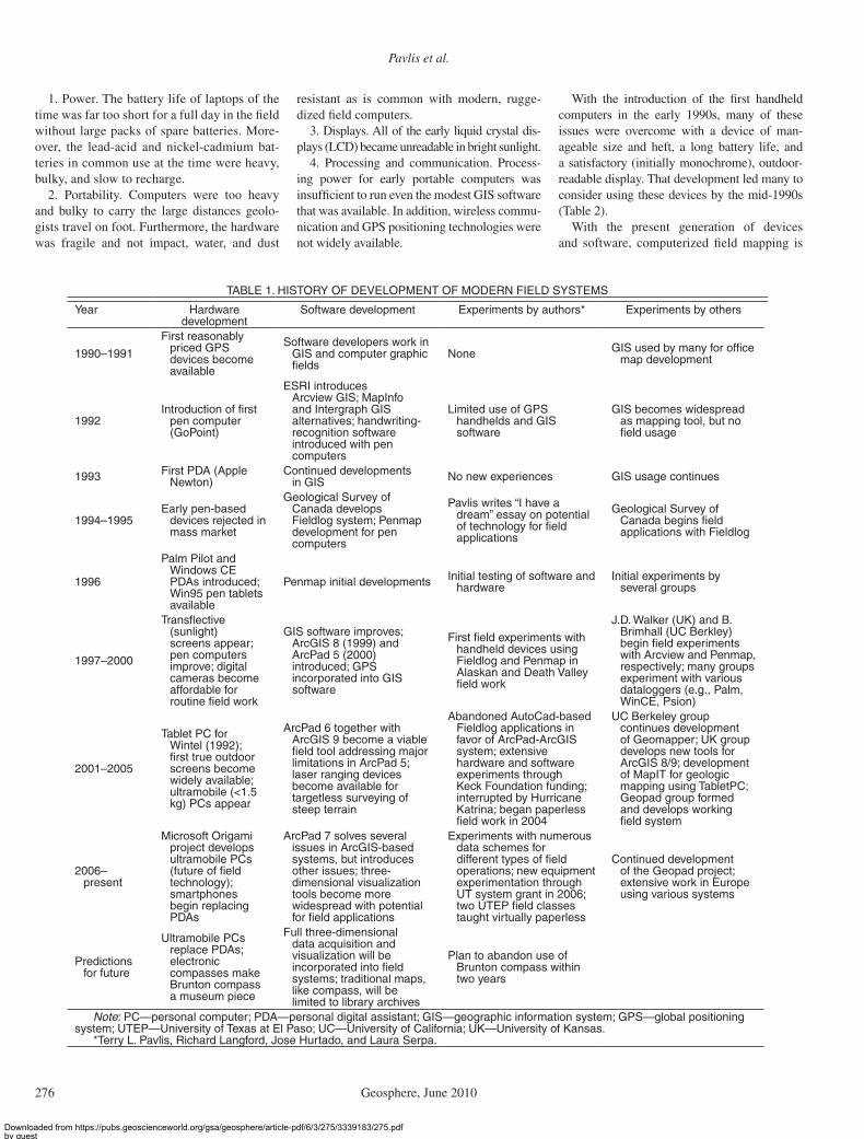
TABLE 1. HISTORY OF DEVELOPMENT OF MODERN FIELD SYSTEMS

Year Hardware development

Software development Experiments by authors* Experiments by others

1990–1991

First reasonably priced GPS devices become available

Software developers work in GIS and computer graphic fi elds

None GIS used by many for offi ce map development

1992Introduction of fi rst

pen computer (GoPoint)

ESRI introduces Arcview GIS; MapInfo and Intergraph GIS alternatives; handwriting-recognition software introduced with pen computers

Limited use of GPS handhelds and GIS software

GIS becomes widespread as mapping tool, but no fi eld usage

1993 First PDA (Apple Newton)

Continued developments in GIS No new experiences GIS usage continues

1994–1995Early pen-based

devices rejected in mass market

Geological Survey of Canada develops Fieldlog system; Penmap development for pen computers

Pavlis writes “I have a dream” essay on potential of technology for fi eld applications

Geological Survey of Canada begins fi eld applications with Fieldlog

1996

Palm Pilot and Windows CE PDAs introduced; Win95 pen tablets available

Penmap initial developments Initial testing of software and hardware

Initial experiments by several groups

1997–2000

Transfl ective (sunlight) screens appear; pen computers improve; digital cameras become affordable for routine fi eld work

GIS software improves; ArcGIS 8 (1999) and ArcPad 5 (2000) introduced; GPS incorporated into GIS software

First fi eld experiments with handheld devices using Fieldlog and Penmap in Alaskan and Death Valley fi eld work

J.D. Walker (UK) and B. Brimhall (UC Berkley) begin fi eld experiments with Arcview and Penmap, respectively; many groups experiment with various dataloggers (e.g., Palm, WinCE, Psion)

2001–2005

Tablet PC for Wintel (1992); fi rst true outdoor screens become widely available; ultramobile (<1.5 kg) PCs appear

ArcPad 6 together with ArcGIS 9 become a viable fi eld tool addressing major limitations in ArcPad 5; laser ranging devices become available for targetless surveying of steep terrain

Abandoned AutoCad-based Fieldlog applications in favor of ArcPad-ArcGIS system; extensive hardware and software experiments through Keck Foundation funding; interrupted by Hurricane Katrina; began paperless fi eld work in 2004

UC Berkeley group continues development of Geomapper; UK group develops new tools for ArcGIS 8/9; development of MapIT for geologic mapping using TabletPC; Geopad group formed and develops working fi eld system

2006–present

Microsoft Origami project develops ultramobile PCs (future of fi eld technology); smartphones begin replacing PDAs

ArcPad 7 solves several issues in ArcGIS-based systems, but introduces other issues; three-dimensional visualization tools become more widespread with potential for fi eld applications

Experiments with numerous data schemes for different types of fi eld operations; new equipment experimentation through UT system grant in 2006; two UTEP fi eld classes taught virtually paperless

Continued development of the Geopad project; extensive work in Europe using various systems

Predictions for future

Ultramobile PCs replace PDAs; electronic compasses make Brunton compass a museum piece

Full three-dimensional data acquisition and visualization will be incorporated into fi eld systems; traditional maps, like compass, will be limited to library archives

Plan to abandon use of Brunton compass within two years

Note: PC—personal computer; PDA—personal digital assistant; GIS—geographic information system; GPS—global positioning system; UTEP—University of Texas at El Paso; UC—University of California; UK—University of Kansas.

*Terry L. Pavlis, Richard Langford, Jose Hurtado, and Laura Serpa.

1. Power. The battery life of laptops of the time was far too short for a full day in the fi eld without large packs of spare batteries. More-over, the lead-acid and nickel-cadmium bat-teries in common use at the time were heavy, bulky, and slow to recharge.

2. Portability. Computers were too heavy and bulky to carry the large distances geolo-gists travel on foot. Furthermore, the hardware was fragile and not impact, water, and dust

resistant as is common with modern, rugge-dized fi eld computers.

3. Displays. All of the early liquid crystal dis-plays (LCD) became unreadable in bright sunlight.

4. Processing and communication. Process-ing power for early portable computers was insuffi cient to run even the modest GIS software that was available. In addition, wireless commu-nication and GPS positioning technologies were not widely available.

With the introduction of the fi rst handheld computers in the early 1990s, many of these issues were overcome with a device of man-ageable size and heft, a long battery life, and a satisfactory (initially monochrome), outdoor-readable display. That development led many to consider using these devices by the mid-1990s (Table 2).

With the present generation of devices and software, computerized fi eld mapping is


Field computer systems

Geosphere, June 2010 277

straightforward and routine. A critical devel-opment has also been the commoditization of GPS positioning devices, which now allow spatial precision not possible as recently as the early 1990s. Other recent developments (Table 2) like automated compass and/or inclinometers, increasing availability of light detection and ranging (LIDAR) data sets, and high- resolution satellite imagery suggest this is only the beginning.

In the mid-1990s, two of us (Pavlis and Serpa) began experimenting with systems that combined handhelds for fi eld data acquisition and standard laptops (including early pen tab-lets) for data compilation (Table 2). This early system used Fieldlog software developed at the Geological Survey of Canada along with a com-mercial software package, Fieldworker, for the Apple Newton handheld (Brodaric, 2004; Bro-daric et al., 2004). This system emphasized a point-based GIS approach where the handhelds and Fieldworker were used for recording point-based observations, and the graphical tasks of mapping were typically done on paper and later digitized using the Fieldlog application. Field-log was essentially a series of applets running under a computer-aided design (CAD) program for database and graphics management. The advantage of the system was that the software was designed with a simple interface for fi eld applications and was intended to insulate the user from the complications of a full-blown GIS system (e.g., see Brodaric, 2004; Pavlis and Little, 2001).

During the late 1990s we experimented with Fieldlog during two research projects, one in Death Valley (e.g., see Guest et al., 2003; Golding-Luckow et al., 2005) and the other in

southern Alaska (e.g., Bruhn et al., 2004; Pav-lis et al., 2004). The dusty, hot dry weather of Death Valley and the cloudy, cold, rainy weather in southern Alaska provided a range of condi-tions in which to test the survivability of the hardware. Because of large power needs of this hardware and the remote wilderness areas in which we were operating, painful power avail-ability issues, which we continue to face today, became apparent. It is interesting that in these fi eld projects we never used ruggedized devices, yet over the course of three fi eld seasons on both projects we experienced only one device failure, amounting to only a one-day data loss.

By the late 1990s, a software package called Penmap (www.Penmap.com) became available. We attempted to use this software as well as a later customized geologic graphical user inter-face (GUI) called Geomapper (Brimhall and Vanegas, 2001; Brimhall et al., 2002, 2006). We also experimented with using Fieldlog on newly available pen tablets in the fi eld. Although they both seemed to be ideal tools, we ultimately rejected both Fieldlog and Penmap largely because of the limitations of pen tablet systems, including (e.g., Pavlis, 1999; Pavlis and Little, 2001) their high cost and excessive weight, and the continued lack of outdoor-readable displays. These problems remain to this day. In addition, Penmap was a relatively “buggy” piece of soft-ware and the Geomapper GUI emphasized a polygon input system that was inconsistent with the approach we had developed independently (see following discussion).

From our perspective, an important advance for fi eld data acquisition came in 2000 when ESRI (formerly Environmental Systems Research Institute, Inc.) released the fi rst ver-

sion of the mobile GIS package, ArcPad. Together with ArcGIS, this software system combined a simplifi ed software interface for fi eld-based data acquisition with a sophisticated GIS for data manipulation in the laboratory or camp. With the release of ArcPad it was also possible to assemble an affordable system for instruction, and as a result, we and others began to experiment with teaching using handheld devices (e.g., Clegg et al., 2006). At the time of this writing we have collectively used variations of this system teaching fi eld geology classes at the University of New Orleans, Massachusetts Institute of Technology, and University of Texas at El Paso (UTEP) with groups ranging between 7 and 15 students. We have also used the sys-tem in day-long fi eld exercises as part of several other classes in groups as large as 22 students. Most important, however, we have contin-ued to use the technology in our fi eld research activities in dozens of fi eld-based projects, and paperless fi eld work is now the norm, not the exception. We have so thoroughly adapted to the system that we now tend to get frustrated with paper mapping as highly ineffi cient with very limiting capabilities.

Collectively, our experience is broad enough that we believe we have probably made most of the likely mistakes one can make in using these systems, and we have developed a practi-cal approach that is exportable to virtually any academic institution. Some key lessons that we have learned from our experimentation include the following.

1. The technology has advanced rapidly in the past 5 yr, and even since Clegg et al. (2006) evaluated these systems. Thus, if someone was introduced to early versions of the technology

TABLE 2. HISTORY OF TECHNOLOGY LEADING TO MODERN FIELD SYSTEMS

Year(s) Computer hardware Technologies applied to fi eld geology

Other relevant technologic developments

Computer applications in geosciences

Early twentieth century

Not yet invented

Aerial photography and derivative topographic maps + transportation revolutionize fi eld work

Major technology advances in numerous subfi elds None

1950s–1960s Primitive computers None Background work in computer

graphics

First use of computers in geosciences, primarily geophysics

1970sFirst

microprocessor computers

Early computer graphics (e.g., stereonet plots, graphical data); no direct fi eld applications outside of geophysics

Key developments in computer graphics lead to GIS; background work leading to GPS

First extensive computer-based applications begin

1980s

Personal computers become widespread; early laptops appear; Psion defi nes PDA and introduces fi rst handheld computer

Computer graphics become widespread for drafting; fi eld use not yet practical because of limitations in both hardware and software

First public domain GIS application (GRASS) and commercial GIS software in 1982—ESRI’s Arcinfo and Intergraph applications; GPS perfected by U.S. Department of Defense

Early computer revolution changes virtually all areas of geosciences with personal computer applications

Note: PDA— personal digital assistant; GIS—geographic information system; GPS—global positioning system.


Pavlis et al.


and found it lacking, we suggest people take a new look at the systems.

2. There are still important, unresolved issues, particularly software limitations, and anyone interested in this technology needs to recognize the time commitments required (see discussion following).

3. Our approach is just one of several, paral-lel approaches to using this technology that have been undertaken. Specifi cally, most of our expe-rience has been in an academic context and we have emphasized systems that are sustainable without a large fi nancial commitment.

WORKING FIELD DATA COLLECTION MODEL

Hardware and Software

We use a system that employs Windows Mobile handheld devices running ArcPad and

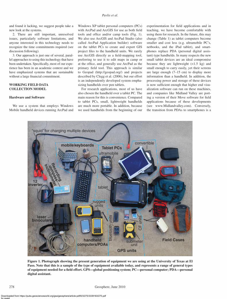
Windows XP tablet personal computers (PCs) with ArcPad and ArcGIS for use as both fi eld tools and offi ce and/or camp tools (Fig. 1). We also use ArcGIS and ArcPad Studio (also called ArcPad Application builder) software on the tablet PCs to create and export GIS project fi les to the handheld units. We rarely use ArcGIS directly as a fi eld-mapping tool, preferring to use it to edit maps in camp or at the offi ce, and generally use ArcPad as the primary fi eld tool. This approach is similar to Geopad (http://geopad.org/) and projects described by Clegg et al. (2006), but our effort is an independently developed system empha-sizing handhelds over pen tablets.

For research applications, most of us have also chosen the handheld over a tablet PC. The main reason for this is convenience. Compared to tablet PCs, small, lightweight handhelds are much more portable. In addition, because we used handhelds from the beginning of our

experimentation for fi eld applications and in teaching, we have become comfortable with using them for research. In the future, this may change (Table 1) as tablet computers become smaller and cost less (e.g. ultramobile PC’s, netbooks, and the iPad tablet), and smart-phones replace PDA (personal digital assis-tant) type handhelds. In many respects the new small tablet devices are an ideal compromise because they are lightweight (<1.5 kg) and small enough to carry easily, yet their screens are large enough (7–15 cm) to display more information than a handheld. In addition, the processing power and storage of these devices is now suffi cient enough that higher end visu-alization software can run on these machines, and companies like Midland Valley are port-ing a version of their Move software for fi eld applications because of these developments (see www.Midlandvalley.com). Conversely, the transition from PDAs to smartphones is a

“squid” for charging multiple devices

laserbinoculars

12inverter

mobile keyboards

Recording

compass-

Inclinometer

handheldcomputers/PDAs

ruggedunits

ultramobile

convertible

tablet

GPS units

Field Casesblue

toot

h un

its

CF

uni

ts

submeterunit

Tablet PCs

Figure 1. Photograph showing the present generation of equipment we are using at the University of Texas at El Paso. Note that this is a sample of the type of equipment available today, and represents a range of general types of equipment needed for a fi eld effort. GPS—global positioning system; PC—personal computer; PDA—personal digital assistant.




negative development because of the smaller screen size of most smart phones and the popu-larity of stylus free touch screens on many of these devices.

For software, we have become fi rm believ-ers in not using a fully featured GIS program like ArcGIS as a fi eld tool. Although ArcGIS is very versatile, its versatility can be a curse in the fi eld because features like cascading menus, right-click requirements, and complex options can produce confusion for anyone but experienced users of the software. Customized interfaces like that employed in the Geopad project (http://geopad.org/) and that of Walker and Black (2000) and Black and Walker (2001) can improve ArcGIS as a fi eld tool, but in our opinion, the program generally is too user hos-tile for the fi eld environment. From our per-spective, ArcPad represents a better fi eld tool because it can be easily customized for the fi eld environment, minimizing the potential for an inexperienced user to become overwhelmed by the software. However, ArcPad is still fl exible enough that it can be adapted in real time in the fi eld. Moreover, while most people can learn the basics of ArcPad in a single 2–3 h training session, few new users would feel even mar-ginally comfortable with ArcGIS in that time frame. Nevertheless, it is important to realize that with ArcPad it is essential that at least one person in a fi eld party has the technical ability to build a project in ArcGIS and ArcPad Studio, to export the project to the handhelds, and to debug occasional software and hardware prob-lems. However, this is generally signifi cantly easier to achieve than assembling an entire fi eld party that is familiar with ArcGIS.

An alternative software product, Map IT (http://www.uniurb.it/ISDA/MAPIT/) was developed in Europe, and Clegg et al. (2006) evaluated its utility for various applications compared to using ArcPad of ca. 2005 vintage. We have not experimented with the software, in large part because it requires use of a tablet PC, but the program has been used in the Geopad project (http://geopad.org/). From descriptions, it appears to be a better choice for geologic mapping applications than ArcGIS, because like ArcPad, it has a simplifi ed GIS front end. Clegg et al. (2006) considered Map IT supe-rior to ArcPad, and although we consider some of the same issues here, their comparison is already somewhat outdated in the latest ver-sions of ArcPad.

Data Structure and Field Workfl ow

An important characteristic of any GIS is that data (attributes or linked information) can be attached to features or groups of features on a map. The ability to attach information to map objects gives the user the ability to change the display based on attributes, overlay transpar-ent layers, or even visualize the data in three dimensions (3D), all of which represents a huge advance in our ability to solve fi eld problems. Although these features are the real strength of GIS, geologists often treat GIS as simply a method for drawing maps. To this day, most dig-ital geologic map releases do not take advantage of the true power of GIS because they typically use minimal attributing. This is particularly true of most regional maps digitized from older paper maps where little, if any, useful informa-tion is attached to the map that was not available on the paper map. A very different type of map can be built, however, when the data are col-lected in digital form in the fi eld with attributing capabilities of GIS in mind.

The fi eld GIS approach introduces a wide variation in possible procedures for fi eld work. Setting up a data structure that takes advantage of the GIS framework is nontrivial, and will require new fi eld habits (e.g., Brodaric et al., 2004). The challenge to a fi eld geologist is to take advantage of this capability while not get-ting bogged down in collecting too much data or ending up with an unworkable mass of poorly organized data (Asch, 2003, 2005).

Early experience with the Fieldlog system quickly taught us that a data structure set up for a laboratory environment is not necessarily workable in a fi eld environment. Specifi cally, a data manager in the offi ce might imagine a data collection scheme that includes a standardized set of data that can be rapidly sorted and ana-lyzed in the offi ce. Unfortunately, if that data scheme is too complex, even the most patient fi eld person will quickly abandon it if each stop involves data entry into multiple pull-down menus with complex pick lists. Thus, all data schemes are ultimately a compromise between the critical data to be attached to map objects in the fi eld and the other data that can be later entered in the laboratory, saving valuable fi eld time. This last point is critical, and often misun-derstood by geologists who have done little fi eld work. Field time is extremely valuable, not only because of real monetary costs, but also because

small increments of lost time can prolong a fi eld project, or lead to poorer results because critical areas might not be visited. As a consequence, we believe the effi ciency of the data scheme used in fi eld data collection systems is critical to the success of fi eld GIS mapping. In particular, three major issues are apparent.1

1. Polygon objects should be avoided. This is because they are too dynamic to build in the fi eld and may require constant reconstruction as mapping progresses. There are a few cases where this rule might be eased, e.g., in surfi cial mapping or bedrock mapping with scattered outcrops. Our experience, however, is that using polygon objects to build a map always leads to diffi culties because of unforeseen topologies that invariably develop. Thus, we use labeling or even hand-coloring of printouts during fi eld work and only build polygons as derivatives after the fi eld work is completed.

2. Keep it simple stupid, or KISS, is an important rule for fi eld GIS systems. Essen-tially, this means simplifying all fi eld data entry to the minimum amount needed for the project. Our rule of thumb is that point objects (e.g., sta-tions) should contain no more than 6–8 attribute fi elds for data entry, and most of these should not be fi elds that are required every time a data point is collected. Examples of high-priority attributes in a station fi le might be: station iden-tifi cation (ID), geologist, date, location method, and a note. For line objects an even stricter rule should be enforced; line objects should contain no more than 3–4 attributes. This rule for line objects arises because attributing can be dis-tracting when drawing the linework on a map. For example, consider the process of drawing a contact that is intermittently exposed with several covered intervals. On paper, this can be performed with little thought. However, in GIS the simplest method for graphic approach is to assign a “quality” attribute fi eld (see sample data), and when a new set of attributes must be entered for each new line segment, it can be frustrating. A second rule is that any pull-down menus with pick lists must contain no more than 6–10 options with no cascading (nested) pull-down menus. Finally, to overcome any limita-tions these guidelines impose, the simple inclu-sion of a “note” fi eld, with adequate space for generic data entry not covered in the fi xed data fi elds, often proves invaluable.

3. Set up the data structure to allow a natu-ral workfl ow in the fi eld. It is crucial to develop

1Supplemental Files 1 and 2. Zipped fi les containing examples of two generic shapefi les that use the data structure described in this paper. The fi les contain two generic projects that, when unpacked, can be used directly in ArcPad 7 or 8. See Appendix 2 for details of working with these fi les. If you are viewing the PDF of this paper or reading it offl ine, please visit the full-text article on www.gsapubs.org or http://dx.doi.org/10.1130/GES00503.S1 and http://dx.doi.org/10.1130/GES00503.S2 to view Supplemental File 1 and Supplemental File 2.


Pavlis et al.


a compromise between display and data entry issues, display always trumping data entry. GIS systems allow data sorting by layers and by attributing data, i.e., assigning values to a data table. Data layers are a fi rst-order attribute and represent one simple way to separate informa-tion, but excessive use of data layers can also be confusing. For most geologic operations we use four types of point objects and 4–10 line types as data layers (Fig. 2). The point objects are sta-tions for noting observations, sample locations, structural measurements, and photographs. The line objects always include the four basic types of geologic contacts: depositional, unconfor-mity, intrusive, and faults. In addition, other structural elements, e.g., foliation traces, thin dikes, and fold axial traces, can be added as lay-ers when needed. These point and line elements are the natural building blocks of geologic mapping, and we typically include each type as a separate data layer, and each data layer is then attributed further (Fig. 2). A sample blank geodatabase and set of shape fi les using this data structure are included herein as an appendix.

Point DataFor many studies virtually all fi eld data are

point observations. Even in areas of exten-sive outcrop, point-based observations are an important part of the fi eld data set, and signifi -cant fi eld time has traditionally been devoted to point-based observations. This is the tradi-tional station approach, in which fi eld notes are keyed to a specifi c map position. We have experimented more with point-based GIS than any other part of the data structure, and our phi-losophy is infl uenced strongly by the approach taken by Brodaric (2004). Nonetheless, formu-lating rules for this part of the data structure puzzle remains diffi cult. This arises in large part because of different styles among fi eld workers; thus, it is diffi cult to establish a data structure that works well for everyone. The data structure shown in Figures 2 and 3 is developed primarily for bedrock mapping, but we believe the basic form of the data structure can be easily molded to other applications. Specifi cally, although we recognize the common use of four types of point data (station notes, photos, samples, and orien-tations), we typically combine the fi rst three into a single station layer and store orientations in a separate layer so that they can be more easily plotted as strike and dip symbols (Fig. 3). From our experience, most of the other point data is archival information that is accessed later and is not useful as part of the fi eld map display. Dur-ing routine mapping we often make the station layer invisible, the computer mapping equiva-lent of using pinholes in paper maps with station numbers written on the back of the map.

Our typical “orientation” data object (Figs. 2 and 3; Appendix 2) illustrates one of these principles. In this fi le we limit data entry to a single strike and dip with the option of including a trend and plunge measurement, and include an attribute fi eld to record the type of orientation data being measured (e.g., bedding versus cleav-age) and a note fi eld to record any subsidiary information. The orientation data are then dis-played directly on the map using layer defi ni-tions imported from ArcGIS. In areas of rela-tively simple structure with only sedimentary bedding, this layer also can serve as the primary data entry form, e.g., a quick record of orienta-tion data to be plotted on the map with a short note on rock unit, or other information.

In more complex areas, however, this simple format may be insuffi cient. For example, in metamorphosed rocks, multiple orientation mea-surements might be made in a small area, and although these data are needed, plotting all these data on the map soon produces confusion. With the recent development of recording digital com-pass and/or inclinometers (http://www.gsinet.co.jp/english/geoclino/index.html), the volume of orientation data obtainable in these types of studies can rapidly grow to unmanageable size. In such cases, we choose which measurement to display using the orientation layer, and we rel-egate all the other data to either a separate data fi le that is later linked into the database, or to the station table. Alternatively, a Boolean “plot to map” fi eld (Fig. 3) can be incorporated into the data structure in ArcGIS. Unfortunately, plotting in the present version of ArcPad is restricted to single attributes, and thus this type of more complex ArcGIS layer defi nition cannot be directly exported to ArcPad.

Other point-based data produce different challenges. Foremost among these is the tradi-tional station, which can serve many purposes, depending on the fi eld project and the individual (Brodaric, 2004). Most geologists are familiar with this type of data object from paper map-ping, but input tends to be a freeform personal preference. What constitutes a station varies among individuals. For example, many fi eld geologists number all stops as stations, while others may use a different code for sample locations versus notes versus orientation mea-surements versus photographs, whereas others may mix all four in various permutations. Thus, although we typically combine station notes, photo descriptions, and samples into one point fi le, this is largely a personal preference. One approach to this issue is the approach used by Brodaric (2004) in Fieldlog. A station object in this approach is the place-keeper for spa-tial position, but the data table for the object is largely composed of metadata, including, e.g.,

a station code, position, date, the person mak-ing the observation. Other data are then linked to this data layer by a common station code, which is written to all associated data tables. In many ways, this is the ideally fl exible system and emphasizes the capability of modern data-base systems (Brodaric, 2004). This approach was used in both a successor to Fieldlog (Geo-fi eld) developed at the Yukon Geological Sur-vey (Lipovsky et al., 2003) and applets devel-oped for ArcPad 6 (Geologic Data Assistant, GDA) developed at the U.S. Geological Survey (Thoms and Haugerud, 2006). Nonetheless, Murphy’s law (i.e., the adage, “anything that can go wrong will go wrong”) always applies to fi eld projects, and we have become hesitant to use this approach because of a hidden poten-tial for data loss. Specifi cally, because all other point data have their spatial reference linked to the station fi le, if that single fi le were to be corrupted there is a high potential for complete data loss. Routine backups minimize this issue, but when using this approach in both GDA and Geofi eld we had partial data losses that required hours of work to reconstruct.

Because of these issues, our recommendation is that station point objects should be set up with a specifi c project in mind, with at least one point object fi le aimed at the specifi cs of the proj-ect. Thus, for projects emphasizing sampling, there should be a specifi c sample fi le, and the other data can be relegated to one or two other objects. Similarly, for bedrock mapping, orien-tation information is often a focus of the work, and thus we typically separate that object in this type of work. Notes tagged to these fi les can also take different forms: text fi elds as a fi eld in the attribute table; linked data fi les defi ned as attributes with the linked fi les representing text fi les, photos, sketches, hand-written notes; and separate data tables.

Line DataMost linework is given a primary attribute

for outcrop quality (exposed, approximate, or concealed). We use that attribute as a primary display parameter in part because of a long tra-dition in geology. However, there is no particu-lar reason that this exact approach be used other than tradition, and the fi eld GIS can allow a more fl exible approach. We have used an expanded list, containing exposed, exposed_projected, approx_fl oat, approx_fl oat_projected, and inferred, the “projected” implying a contact that is extended using aerial photography or sketch-ing from a distance. We have experimented with a quantitative attribute for contact quality (e.g., <10 m, 30 m, inferred), but found that this pro-cedure confused people familiar with the con-ventional map scheme.




Point Shapefiles

Line Shapefiles

Figure 2. Examples of typical data entry screens for our ArcPad projects. See text for discussion.


Pavlis et al.


Station feature class(spatial position

typically captured by GPS)

p.1: principal facts

Stationnumber___Date___Geologist___LocationMethod___Outcropquality___other options:map unit, weather,etc.

p. 2: linked informationp. 3-5: Notes

(250 character fields)

photofilename ____photo caption____sample_________sample desc____long note (y/n)longnotefile____

1

11

Can be automated2

22

Pull down menu item

3

3

File name generally not completed in field

4

4

4

Boolean (y or n field)

note1 note2 note3





# of photos___# of samples_____

long note (y/n)longnotefile____

1

11

Can be automated2

22

Pull down menu item

3

3


4

4

Boolean (y or n field)

p. 3 photo descriptions

p. 4 sample descriptions

p. 5 short note

Generic Station Table Data Structure

Alternative 1: Sample or photo intensive stations





# of photos___# of samples_____long note (y/n)longnotefile____

orientation datatable ____

1

11

Can be automated2

22

Pull down menu item

3

3


4

5

4,5

4

Boolean (y or n field) Linked orientation data could be generated as a spreadsheet, text, ordatabase table from another application;Can also be ignored and “longnote” usedin place of a separate data table, dependingon the application needed

p. 3 photo descriptions

p. 4 sample descriptions

p. 5 short note

Alternative 2: Orientation data intensive stations (e.g. detailed structural studies)

Limitations: with this data structure multiple samples or photos at a station need to berecorded in notes, with information linked later in the lab.

Note: longnote file name refers to the file name of notes entered in word processor +/- sketchesembedded in the long note. File name can be entered, but commonly will need to be linked to the database later, not in the field Figure 3. Illustration of alter-

native data structures for station fi les. Example fi les included with this paper use the data structure illustrated at the top of the fi gure, but the other alternatives have been used successfully. GPS—global positioning system.




Depending on the project being undertaken, a number of other attributes can be given to linework. For mapping in sedimentary rocks (e.g., Figs. 2 and 3) we have commonly used a “contact type” attribute. In an area with well-established stratigraphic units, this attribute can be used to defi ne the standard contact, but for areas with poor stratigraphic control or thick units, we also include a “sedimentary_ bedding_trace” attribute to identify the line as an intra-formational bedding surface trace distinct from a traditional formational boundary (Fig. 4). For detailed sedimentary studies, sequence bound-aries, fl ooding surfaces, and hierarchical bound-ing surfaces can also be added. The ability to zoom into a small area is particularly important for mapping smaller scale features, such as bounding surfaces, because until now, these sur-faces typically have been traced only on outcrop photos. Alternatively, in volcanic rocks, or areas with volcanic rocks interbedded with sedimen-tary rocks, the contact type attribute can be used to distinguish volcanic versus sedimentary con-tacts. We always include a note attribute with a large data fi eld where additional information can be added. This information is the type of narra-tive or descriptive material a geologist would traditionally write in their fi eld notebook. It is interesting that having this recorded digitally as an attribute of a specifi c GIS object ultimately changes many people’s note-taking habits. Spe-cifi cally, the note fi eld for an individual line element can be used to add information about the feature that could never be done with paper mapping. For example, notes like “this con-tact is speculative” or “this is accurate to ~1 m through GPS positioning and high-resolution aerial photography,” are possible.

Working in metamorphic rocks leads to a somewhat different linework data structure (Fig. 5), where more complex attributing may be needed to allow a particular type of data display. Similar issues also arise in economic geology (Brimhall et al., 2006). For example, in com-plexly deformed metamorphic terranes, in addi-tion to primary compositional layering, there is typically more than one structural fabric (e.g., S0, S1, S2) and surface traces of these features can be routinely mapped. It may also be desir-able to map other structural elements (e.g., axial traces of multiple fold generations, linear fabric traces), and features such as metamorphic iso-grads or hydrothermal alteration zones. Because these fi eld GIS systems allow us to simultane-ously map and selectively display these multiple surfaces, it is in these environments where we have found the most profound improvement over traditional paper-based mapping.

Because there are so many lines (each poten-tially with several attributes) being drawn on a

map, implementing a fi eld GIS system for meta-morphic and economic geology work strongly underscores the KISS rule. We have typically settled on a simplifi ed data structure with a data layer for each linetype (e.g., S0, S1, S2), each with no more than two basic attributes (quality and note), and with no requirement that these attributes be set in the fi eld. In practice, to speed fi eld operations, we generally do not attach any attributes for foliation traces other than layering and we use notes or photographs to clarify the quality of the mapping. In this case, attributes can be added later, including linework groupings in an ArcGIS geodatabase, to clarify the nature of the information. For fold systems it is tempt-ing to develop a complex data structure that would encompass the entire range of possible fold types, a strategy that in practice becomes unworkable. Thus, for folds we use only one layer for fold axial traces, typically limiting the fi elds to an attribute for graphical display. In our sample data fi le, for example, we use only a fold form attribute, and other data (including fold generation, orientations) are entered in a long note fi eld. An alternative data structure is to use both a form and generation attribute, but the assignment of folds to generations routinely can cause confusion if this approach is used in a new fi eld area where generation assignments may be in fl ux for days.

Data Compilation and Note Correlation

An important element in GIS-based fi eld studies is compilation at the end of the day, which includes both routine backups and data entry and/or repair. The procedure can be as simple as downloading a digital camera, chang-ing fi le names, and linking the photos to the database. However, more complex procedures can be developed, including revision of line-work using aerial photography, digital eleva-tion model (DEM) shaded reliefs, or both, as well as editing attribute tables. These editing operations are all GIS-related functions that can be done outside the fi eld environment, and the extent of this exercise depends on the proj-ect, the personnel in a project, and the preferred procedures for the group. This editorial step, however, is critical, and is the digital equivalent of “inking of lines” or daily map compilations. Conceptually, this step can be very important for both students and a researcher as a refl ec-tion on the day’s work, is crucial in planning for the next day, and can be a critical meta-cognitive step in fi eld problem solving (e.g., http://serc.carleton.edu/NAGTWorkshops/metacognition/index.html).

In our experience, it is important to evalu-ate the fi eld project at hand, the fi eld personnel,

and the project’s specifi c needs, in determining how much effort is spent on daily data compi-lations and/or editing versus fi eld data entry versus post–fi eld work data compilation and/or editing. If a fi eld project is working in a remote site, evening fi eld time may be limited, and thus, required evening data compilation and/or editing should be minimized. Alternatively, if a project has extensive logistical support (offi ce and/or room for evening work with no power limita-tions), fi eld efforts can be maximized by delay-ing many steps to evening data compilation.

Similarly, there are hybrid fi eld procedures that may be appropriate, depending on indi-vidual preferences. For example, we have found many people prefer to use a traditional paper notebook in the fi eld for developing sketches and notes, minimizing data entry in the fi eld. For teaching applications this may be a pre-ferred technique to encourage good note taking. However, when this type of hybrid approach is used, it magnifi es the need for evening data compilations; either forcing evening data entry or at least correlation of notebook entries to the digital data fi les.

Logistical Issues for Computer-Based Field Projects

Field geology projects are often undertaken in remote areas where electrical power is limited (or nonexistent) and where environmental con-ditions can take a harsh toll on electronics. Both of these issues are closely related.

Since most hardware has, at most, three days of useful battery life, a fi eld party needs to develop a plan for keeping equipment opera-tional that includes redundancies in the event of equipment failures. In group exercises for geology fi eld classes, this may require some-thing as elaborate as a generator, and multiple power outlets for charging devices. For smaller groups or applications in extremely remote areas, the best power solution we have found is solar-powered, portable 12 V charging systems. Careful consideration, however, must be placed to balance space and/or weight limitations with power needs. This is problematic since fi rst-time users are unfamiliar with how to budget the wattage per day required, the critical criterion for selecting the size solar panel required. Simi-larly, most car batteries are a poor choice for a solar charging system because they are gener-ally prohibited in aviation cargo, cannot tolerate deep-cycling, and they typically have a much larger capacity than needed. From our experi-ence, a fi eld party of 2–4 can be maintained with a sealed 10–15Ahr battery charged with a 20–40 W solar panel. A critical piece of electronics that is often overlooked in constructing a solar


Pavlis et al.


((

.

..

oo

45

48

53

7387

87

4080

85

59

62

898979

6921

46

3342

86

42

37

300 0 300150Meters 1:12,000

Figure 4. Example of an ArcGIS map generated using our digital mapping techniques. Figure illustrates the power of digital mapping to develop extensive linework on a map beyond traditional mapping, here illustrated as a bedding-plane-trace map. Note that in this area, mapping of only the traditional forma-tion boundaries (heavy black lines) and faults would have produced a map with little useful information, whereas inclusion of the bedding traces shows the structure in detail. The map is from southern Alaska in the fold-thrust belt of the St. Elias Range, just east of Bering Glacier (our data).




charging system is a voltage regulator to avoid destroying a battery by overcharging, a device readily obtained from businesses that sell solar power equipment.

The physical environment (e.g., weather, alti-tude, wildlife) requires logistical planning simi-lar to that required for geophysical fi eld experi-ments. Weather issues, for example, affect the kind of power system that is most practical for a project. For example, preventing short circuits in a wet environment is a fundamentally differ-ent challenge than working in a desert where dust and sand might clog terminals and cooling fans. Equally important is that someone in the fi eld party takes the responsibility of technical expert. That person must be knowledgeable enough to maintain all equipment in working order. Appendix 3 gives a simple checklist of useful spare equipment, tools, and suggestions for troubleshooting.

As a fi nal logistical note, geologists should not proceed to a remote location until they have

spent several days of actual mapping in an area where they have access to high-tech support—software, hardware, or both. The list of potential problems is long when users are unfamiliar with the system. Thus, new users need to gain experi-ence with the equipment in an area where there are no time pressures and high-tech resources are available, not in a remote site with limited or no communication.

DISCUSSION

Field geologists have a poor record of devel-oping collaborative fi eld efforts, a tradition that goes back to Roderick Murchison and Adam Sedgwick’s well-known feud in the nineteenth century. This problem arises from the basic nature of traditional fi eld work. First, geologic maps are a derivative of a series of point obser-vations, each of which can be subject to random chance and subjective interpretation (e.g., Ernst, 2006). As a result, a geologic map becomes

“fuzzy data” wherein facts are mixed with inter-pretation. Second, collecting basic fi eld data is laborious and, in some cases, dangerous. As a result, the intellectual property encapsulated by a geologic map has a very high value to the pro-ducer of the map, yet to the broader community the information is merely a part of a broader col-lection of knowledge.

We suggest that if all fi eld geologists began to use the type of GIS system described here and elsewhere (e.g., Clegg et al., 2006; Brimhall et al., 2006), the community would ultimately develop a different attitude about fi eld data. The “fuzzy data” issue can be entirely eliminated because in a GIS there can be an explicit segre-gation between objective, quantitative data col-lection and subjective data interpretation. The basic data used to develop a map, such as fi eld descriptions, photographs, and orientation data, can always be extracted from the database. Fur-thermore, if the basic fi eld data are always col-lected in digital form within a GIS, the data are

A

Figure 5 (continued on following page). Example of the power of digital mapping in analysis of the complex structure of metamorphic terranes. (A) ArcPad dialogue boxes using the sample data fi les accompanying this paper.


Pavlis et al.


inherently archival, and ultimately can be easily shared with the broader community. This data-base would also allow other workers to directly examine the basic observations that support the geologic interpretations on the map. This is a remarkable advance in how fi eld geology is done because it greatly facilitates the equivalent of reproducing an experiment in other branches of science.

How fi eld data are archived is beyond the scope of this paper, but we believe that it is imperative that this problem is addressed in the near future. Clearly there is a time window

during which fi eld data should be the sole intel-lectual property of the scientist who produced it. After a project is completed and main results published, however, it is a waste for that infor-mation to disappear into a fi le drawer, which is the typical case today. Thus, it should become a routine procedure to archive basic geologic data as we move into digital mapping. The ease of data archival in a GIS format makes this a straightforward process, but the data structure of the archival information is not. The U.S. Geological Survey has developed one archival model (http://ngmdb.usgs.gov/Info/standards/

NCGMP09/) that minimizes required attributes in the GIS but allows more extensive attri-butes in nonstandard fi elds. Although this “one size fi ts all” approach is an important step for regional map compilations in a large organiza-tion (Haugerud et al., 2009; Thoms et al., 2009), there are undoubtedly complications in detail as these systems evolve. It is important for the broad geoscience community to contribute to these evolving issues because although the stan-dardization of data structure for data release is important, in fi eld systems a standardized data structure may stifl e creativity.

Standard Geologic Map with foliation traces

Foliation traces S2 foliation only Foliation traces S3 foliation only

Standard Geologic Map with foliation tracesand Quaternary removed for clarity

B

Figure 5 (continued). (B) A series of screen shots of a digital geologic mapping prepared with different data layers that can be turned on or off to display different structural generations (from Pavlis and Sisson, 2003).




Suggested Changes in Field Procedures

In using fi eld GIS technology we have con-cluded that a number of long-held paradigms for fi eld work need to be reexamined. This extends not only to the research environment but also to the way we teach fi eld geology to undergraduates.

A paradigm of fi eld geology has been that when you leave the fi eld on a given day, all linework should be complete. This paradigm is so fi rmly entrenched that it is a mantra empha-sized in virtually all fi eld geology classes at the undergraduate level. We suggest that although it is still critical to impress on students the need to complete linework and descriptions in the fi eld while the geology is in sight, overem-phasis on this concept can be a handicap when using modern technology. Specifi cally, in the interest of increasing fi eld effi ciency, some fi eld tasks are best accomplished as an itera-tive process of fi eld observations, cleanup, and further fi eld observations.

In conventional paper-based mapping, the mapping process began by referring to any previous geologic mapping, and these maps might or might not be carried into the fi eld for appraisal. In the fi eld, the typical procedure would be to map directly onto a topographic map, aided by aerial photography if available. In some cases, orthorectifi ed aerial photographs (or satellite imagery) could be used with or without a topographic map overlay, but gener-ally most geologists carry imagery as sepa-rate stereo pairs. The result of having so many disparate paper map products was the “fi eld map shuffl e”; i.e., constantly looking from old geologic map to topographic base map to aerial photographs, to the landscape in front of you, back to the topographic map, and so on. Although anyone who has done extensive fi eld work becomes accustomed to this procedure, it is inherently ineffi cient. In contrast, the ability to stack multiple, georeferenced data sets on a computer screen, including options to make lay-ers transparent, avoids the fi eld map shuffl e, and allows the fi eldworker to concentrate on the task at hand: understanding the local geologic rela-tionships. Moreover, when the data are acquired as fi rst-generation digital maps, many compila-tion errors can be directly avoided (e.g., map compilation blunders and confl icts discussed by Campbell et al., 2005).

The availability of multiple, georeferenced data layers in a fi eld GIS also leads to a differ-ent workfl ow. In particular, even before going to the fi eld, data compilation from existing maps and photointerpretation of imagery can lead to a partially completed geologic map. Field work can then concentrate on specifi c problem areas,

clarifi cation of fi eld relationships, and testing of hypotheses. In a very mature area, fi eld work might be limited to refi ning details, but in less well known areas, the fi eld work would require more extensive geologic mapping. In either case, however, the preliminary work saves and enhances the productivity of valuable fi eld time.

The iterative nature of collecting and devel-oping fi eld data in a GIS is also different from paper mapping. Paper maps are always refi ned and modifi ed (with pencil and an eraser) during fi eld work, and many people compile the infor-mation nightly to a base map. In the computer mapping world, this last step, compilation, is a necessary and potentially major contributor to the effi ciency of fi eld work. At a minimum, the tedious work of daily backups of data and cataloging and renaming of data fi les (i.e., pho-tos, orientation data fi les) is essential, but other steps at this stage can be very informative. For example, when good aerial photographs are available it is often more effi cient to not worry about precise details like exact contact place-ments while in the fi eld, particularly when time is an issue. Instead, roughing out the basic line-work with some careful georeferencing of criti-cal points may be all that is necessary, and in the evening the map can be cleaned up and refi ned, particularly projected contacts, using the aerial photography (Fig. 6). Depending on the quality of imagery and abilities of the fi eld geologist, this procedure can usually be completed in less than an hour each evening.

This suggestion will undoubtedly appall many long-time fi eld geology instructors, but if one has not used these systems it is diffi cult to appreciate how effi cient this procedure can be. In recent undergraduate fi eld geology classes at UTEP we were surprised by the dramatic improvement in the quality of student maps pro-duced with this technique. The lead author had used this technique for some time in research environments, but the impact on a research set-ting is less obvious than that on students because the high skill level of research personnel primar-ily led to fi ne tuning of maps in the compilation stage. With the lower skill levels of students, however, the impact was dramatic because stu-dents quickly saw their errors on high-quality imagery when they had time to view their work without the multitasking pressures of the fi eld day. We suspect that this improvement is due to students taking a more active role in planning and daily refl ection on their work, an impor-tant metacognitive step in learning (e.g., see http://serc.carleton.edu/NAGTWorkshops/metacognition/index.html), and is consistent with Riggs et al. (2009) observations of student success when fi eld planning was used by suc-cessful students in fi eld classes. Nonetheless, the

success of this method has not been universal, because one of our recent fi eld classes performed poorly with this approach. In this case, the prob-lem appears to have originated when students became accustomed to using aerial photography where rock units were clear on the photos, but when confronted with an area where photo inter-pretation was diffi cult, they experienced major problems. We do not have a clear solution to this problem, and it represents a geoscience educa-tion issue that needs to be addressed.

The process of data compilation and fi nal map preparation is a critical step in fi eld GIS map-ping that, if ignored, can lead to less geologic insight than paper-based mapping. Although the old-fashioned processes of compilation, ink-ing, and map coloring are tedious, for most of us, this process was an intellectually important step in data synthesis. It forces appraisal of map patterns and evaluation of accuracy, particularly when linked to analyses such as cross-section construction: that is, a metacognitive step simi-lar to that described above. In a computer-based mapping system, the tedium of the compilation and fi nal map preparation step can be largely eliminated. At the same time, however, the data synthesis function of this step can be retained and enhanced. Along with conventional cross-section construction, we have used two other procedures to aid this step: (1) topology build-ing and editing, and (2) 3D visualization.

We noted here that we typically avoid poly-gons during geologic mapping, largely to avoid wasting fi eld time on a process done more eas-ily in the lab. However, there is also an intel-lectual advantage to delaying this step. In the GIS approach, this step represents the digital equivalent of coloring a map. Like coloring a map, this step forces map appraisal line by line through cleanup of map topology, and forces a close look at the map to aid visualization. The frequency of this step depends on personal choice. This step can be done nightly if a project is fully integrated into a GIS, or it can even be done continuously if ArcGIS is used as a fi eld tool (e.g., Walker and Black, 2000; Black and Walker, 2001). However, it can also be delayed indefi nitely, and if a group is not comfortable with GIS software, old-fashioned hand-coloring of printouts can serve the same purpose.

Finally, 3D visualization systems represent the ultimate future for fi eld geology, but at the time of this writing there is no practical sys-tem that is useful for the fi eld environment. In particular, true 3D displays are limited to the laboratory environment and the only 3D tools available for fi eld work are pseudo-3D applica-tions using perspective views; e.g., web-based systems like Google Earth, and viewers like iView3D and ArcScene. Similarly, although


Pavlis et al.


A

B

Figure 6. Example of raw fi eld maps generated using ArcPad as fi eld tool with evening edits in Arc-GIS. The fi gures show linework plotted on an orthophoto base. A) Linework after completion of a day’s mapping, with pink lines showing bedding traces at the completion of the day’s fi eld work and green lines showing changes in that linework completed that eve-ning (bright red lines—faults; blue lines—unconformities; and map-ping faults and unconformities shown had been completed during previous work in the area). B) The fi nal map after the evening’s edits. Note how initial fi eld linework was refi ned, particularly in areas of low dip in left-center and lower-central parts of the map. Comple-tion of this linework in the evening saved valuable fi eld time in this area of good exposure, illustrating the power of the technique for fi eld effi ciency as well as accuracy. The map area is in the Indio Moun-tains south of Van Horn, Texas, with an extensional half-graben in the central part of the map bound by a low-angle, southwest-dipping normal fault (red line) to the northeast and an unconformity to the southwest. The structure below the unconformity is a Meso-zoic fold-thrust system.




some software, like Move from Midland Valley Exploration software (http://www.mve.com/), allows true 3D digitizing, this software requires special licensing and is expensive for nonaca-demic units. Nonetheless, Midland Valley is developing this software for fi eld applications and has signifi cant promise. New software developments in the UK (e.g., Mathers et al., 2009) and experimentation in the U.S. (e.g., Phelps et al., 2009) offer a future for 3D mapping at a variety of scales, but remain an offi ce tool. Thus, fi eld geology must await future develop-ments to fully integrate 3D into the fi eld envi-ronment, particularly hardware such as heads-up displays, 3D displays for mobile devices, and augmented reality systems. Nonetheless, 3D visualization can be used as part of evening map compilation work, depending on the logis-tics of a fi eld project. For example, we have used Google Earth to aid in data compilation in the evening with classes. In research settings we have used ArcScene and the commercial program Fledermaus (http://www.ivs3d.com) to drape shapefi les and published geologic maps onto a DEM, and used 3D viewing capa-bilities to help recognize mapping errors and clean up mapping (Fig. 7).

Future Revolution in Field Geology—Examples

Metamorphic GeologyThe structural geometry that can be pro-

duced by multiple generations of fold over-printing in metamorphic terranes represents one of the most diffi cult 3D visualization prob-lems in all of geology. Traditionally one of the main methods for resolving geometry has been systematic mapping of the surfaces traces of different generations of structural fabrics (e.g., Hobbs et al., 1976, p. 347–375) together with symmetry analyses (stereographic projection) and cross-section construction. The fi eld pro-cedure is time consuming, and in conventional paper mapping often produces a map that is completely incomprehensible to anyone but the person who made the map. In contrast, fi eld GIS provides the ability to superimpose multiple data layers, turn layers on and off, and zoom a fi eld map through a nearly infi -nite scale range, all of which are mapping functions that are a remarkable improvement to anyone who has done this kind of mapping on paper. Furthermore, the recently developed digital recording compass inclinometer opens options never before considered. These devices can rapidly measure orientations of planes, or simultaneously measure the orientation of a plane and a line on the plane. We used one of these devices recently and obtained as many as

100 plane-line pairs in less than an hour. This suggests that unprecedented geometric resolu-tion can now be done routinely. When com-bined with high-resolution GPS this could lead to a whole range of new capabilities in resolv-ing complex geometries. As 3D visualization systems develop further, the capabilities of resolving complex structural geometry will only improve, and we predict a future revolu-tion in our understanding of complex meta-morphic structures as a result.

Sedimentary GeologyThe combination of GPS with a fi eld GIS

also creates new opportunities in sedimentary geology. Sedimentary features are typically analyzed as 2D objects. Although the advent of sedimentary architectural studies and sequence stratigraphy has highlighted the 3D nature of sedimentary features, understanding of the 3D geometry is handicapped by limitations of both data collection methods and ability to visualize the systems. Today, many scientists are experi-menting with ground-based LIDAR systems, laser rangefi nder systems, high-precision GPS, or some combination of these technologies. However, these represent only a part of the tools needed to best resolve true 3D architecture. Mapping using a fi eld GIS system allows for huge improvements in the development of true 3D reconstructions. Simple tracing of bedding planes becomes a 3D exercise that, in combina-tion with a 3D imaging program, can revolution-ize our understanding of sedimentary systems. Using these tools together with a GIS mapping system represents a powerful combination that is diffi cult to overemphasize.

Planetary GeologyMany of the lessons we learn from terrestrial

work with fi eld computing systems can have a direct bearing on how these systems could, and should, be developed for fi eld science on the moon, Mars, and beyond. These missions will present serious challenges that go far beyond the most hostile environments encountered by fi eld geologists. Field GIS technology can greatly enable fi eld exploration in hostile plan-etary environments where the geologist will be hampered by both terrain and the need to carry a life-support system that puts severe constraints on time and metabolic activity.

Properly implemented, a fi eld computing system not unlike the one currently in use by us can streamline and simplify the information resources needed during an extravehicular activ-ity (EVA), or spacewalk. This can include both the operational checklists required to safely per-form the EVA as well as the data-gathering tasks, e.g., geologic mapping and sample collection, to

be accomplished during the EVA. In addition to the added effi ciency afforded, some tasks that would otherwise be unfeasible would be made possible. For example, during the Apollo mis-sions, the astronauts did not have the capabil-ity to map geologic contacts and were limited to verbal descriptions of geologic relationships and the collection of samples. With a fi eld GIS system coupled to a geolocation capability anal-ogous to GPS, future astronauts could precisely map out the geometry of geologic relationships in the fi eld by simply walking them out, or by digitizing them from distance with a laser range-fi nder. Numerical data and descriptions (trans-lated to text via speak recognition), in addition to digital photography, could be linked to the fi eld GIS, just as easily as they can now with ArcPad. In addition, the fi eld GIS system would allow the full use of available remotely sensed data as a base map for both scientifi c decision making and for navigation.

These enhanced capabilities will also encour-age complete documentation and curation of fi eld data and samples, crucial tasks for activi-ties in locations that are expensive and diffi cult to reach. For example, when fi eld data are col-lected in a GIS, (near) real-time transmission and remote analysis and/or archival of that GIS data are possible. This can allow the support staff on Earth to vicariously explore and better engage and/or direct the astronauts during any EVA and enable better planning between EVAs. This can also allow richer sharing of informa-tion among astronauts in the fi eld, supplement-ing the voice communications with real-time data and further increasing effi ciency in the fi eld in terms of time, metabolic costs, and amount of ground covered.

Implications for Teaching Field Geology

Although we have described some issues related to teaching with fi eld computer systems, a number of additional issues are important to emphasize. All students have different ways of learning, and in traditional fi eld geology classes there is little room for alternative learning tech-niques. That is, there is no other way to collect data than to go to the fi eld. During fi eld classes there is a widespread “sink or swim” attitude that places many students from urban environ-ments or with physical limitations at a great disadvantage. Using fi eld computer systems allows a great deal more fl exibility in data col-lection that can benefi t these students in par-ticular. Foremost among these capabilities is the potential of 3D visualization systems to permit virtual access to any place on Earth. Through these systems there is tremendous instructional potential for both students with no direct access


Pavlis et al.


near-vertical, oblique view

View down-plunge of folds

Figure 7. Split-screen stereo views of a fi eld area in southern Alaska showing the power of three-dimensional (3D) visualiza-tion with these systems. Yellow lines are bedding traces and red lines are faults. For more details, see the ivs fi les (included herein) of the same data set. Figure was prepared using digital fi les generated during fi eld work in the area, refi ned and edited in ArcGIS using high-resolution imagery and light detection and ranging (LIDAR) topography, draping of the shapefi les onto a LIDAR digital elevation model (DEM) using Fledermaus (see text), and using the Fledermaus viewer for split-screen stereo (e.g., Geowall display). Although this is an elaborate example, similar capabilities can be easily extended to any fi eld project, particularly as 3D display capabilities improve.




to geologic features near home and for physi-cally disadvantaged students. Anyone who has taught fi eld geology is familiar with situations where a student either arrives or becomes physi-cally incapable of conducting day-to-day fi eld work, and using visualization is one way to deal with this issue.

Another teaching benefi t we have found is the ability to encourage collaborative learning with the use of the fi eld GIS systems. In a sense, fi eld geology classes have long employed some form of collaborative learning in the use of fi eld partners, although working in pairs primarily serves as a safety factor. Nonetheless, students working in the fi eld in pairs or in groups have long lead to assessment nightmares because it is often unclear whose work ends up in the fi nal result. Field GIS systems do not eliminate all of these problems, but do improve our ability to assess individual performance because students can be asked to present their raw data fi les at any time during a fi eld project.

More important, however, using fi eld GIS systems can encourage true cooperative proj-ects and team-building exercises where stu-dents can gain familiarity with working in a group research environment. For example, many fi eld classes have long emphasized a research approach to fi eld problems and used groups of students to develop regional geologic maps where student groups were responsible for all steps from data production to data com-pilation. Although this approach is possible with a traditional paper mapping approach, it is far easier to implement with a fi eld GIS system. With fi eld GIS, student maps can more easily be merged to produce an aggregated data set that covers a large area. Students can discuss and revise the maps as they compile the data, and peer pressure can force improved perfor-mance when the group is relying on input from everyone in the group. Thus, use of computer-ized systems can encourage a research quality approach in fi eld classes.

A second advantage of using these systems for teaching is the accelerated learning of several key fi eld skills. One clear example we have seen is, by incorporating GPS positioning for station descriptions, students more quickly adapt to the fi eld techniques of station description and orien-tation data collection without the classic question of “where am I?”: unfortunately, it is not clear that this step improves performance on other mapping skills, because the traditional “where am I” question also serves to improve map read-ing skills that are essential for things like pro-jecting contacts. Moreover, we have recognized cases where some students experience signifi cant problems with synthesis exercises, and we sus-pect the small screen size of handheld computers

may be a culprit (e.g., see discussion by Clegg et al., 2006). In the future we plan to experiment with techniques to force continued data synthe-sis, but we are uncertain of the ideal approach. We suggest that fi eld classes should experiment with different techniques that can aid accelerated learning of fi eld techniques, but should recog-nize the variety of learning techniques among the students. We suspect that as 3D visualization becomes more widely available, the 3D visual-ization system, together with GPS, will make a powerful accelerated learning tool. Thus, we sug-gest that collectively these are important research issues for geoscience educators.

CONCLUSIONS

Our experiences with fi eld GIS mapping systems indicate that they are a signifi cant improvement over the traditional paper map-ping techniques that have dominated geol-ogy for more than two centuries. In particular, instrumentation and techniques now exist to collect large amounts of data rapidly and with high precision in the fi eld. More importantly, those data can be merged and viewed with a variety of other geospatial information, both in and out of the fi eld setting. This makes the fi eld mapping process much more effi cient and increases the reliability and repeatability of col-lected data. The ability to combine data sets and create 3D visualizations of mapped structures increases the interpretive abilities of the map-per, both in and out of the fi eld.

There are some trade-offs that arise when using computers in mapping. In particular, the user must know something about the software and hardware as well as implement new proce-dures to prevent the loss of data in the fi eld. We have found, however, that we can teach under-graduates, even those with little computer back-ground, the necessary skills in a short amount of time. We note, though, that in any fi eld effort, one or more people must be relatively skilled at all aspects of the software and hardware to avoid catastrophic results. Becoming profi cient in using these systems requires a different learn-ing procedure than paper mapping. Everyone is familiar with paper and pencil since childhood, but not everyone is comfortable with using these high-tech devices. In teaching students the sys-tems accelerate learning in some areas, but can produce obstacles in other areas. For experi-enced fi eld workers the steep learning curve of adapting to the systems will initially seem an obstacle, but it is well worth the effort once you have learned the system.

The time has come to abandon paper-based mapping, and we hope that within a decade we will look back on geologic mapping using

a Brunton compass and paper maps as a quaint artifact of the past, reminiscent of the plane table and alidade for mapping, the blow-pipe for mineral analysis, or other archaic technologies.

APPENDIX 1. NOTES ON HARDWARE SELECTION

Hardware suitable for fi eld situations depends heavily on the use planned for the systems, and for the physical environment of the fi eld work. We rec-ognize three key issues for selecting hardware: (1) ruggedization; (2) display; and (3) weight.

Ruggedization

Although it is tempting to assume that all fi eld work requires so-called ruggedized devices, from our expe-rience these devices are generally a waste of money. In more than 10 yr of working with these devices we have physically broken only two devices and one of these was a rugged device, which, ironically, cost more to repair than a new nonrugged device. Electron-ics failure independent of accident, however, is more common; e.g., in our experience, ~10% of handhelds undergo a hardware failure within 2 yr. Fortunately, the consequences of fi eld hardware failures can be minimized by using interchangeable fl ash memory devices. That is, we keep all data fi les on secure digi-tal (SD) or compact fl ash cards, which can be removed in the event of a hardware failure. Note, however, that these cards also fail periodically, and thus backup to other media is also critical to ensure data integrity. We have found that fl ash card failures can be minimized if fi les are completely rewritten daily to avoid repeated rewrite cycles on the same sector of the card. There are several methods to accomplish this, but the easiest method is to move each day’s work into new folders, particularly if nightly edits are performed.

Display

There remains a complete range of display types available for fi eld devices, but currently the princi-pal distinctions in usable outdoor displays is trans-missive versus transfl ective displays. Conventional LCD displays on laptops use a transmissive display, and use a backlight to make the screen viewable. In an outdoor environment, a transmissive display can produce a reasonable display, but usually requires a very bright backlight, a situation that produces a trade-off between display quality and battery life since the display produces a large power drain. We have found these types of displays acceptable if the main work environment allows access to shade or the work is in cloudy areas. In direct sunlight, none of these types of displays produces a legible display.

In contrast, transfl ective displays work best in direct sunlight, and in the shade or on cloudy days, require use of a backlight for clear visibility. As the name implies, these displays have a refl ective LCD panel and a subtle issue with these screens is the screen surface. Many devices come with a nonrefl ec-tive coating, which improves display dramatically by minimizing glare, yet these devices often contain a dilemma; for practical fi eld use, a screen protector is required to avoid destroying surface coatings with the pen interface, yet most screen protectors lack nonre-fl ective coatings. There is currently no solution to this


Pavlis et al.


problem other than to avoid devices that rely heavily on screen coatings for glare suppression; although rare, some screen protectors have some glare suppres-sion, although usually at the expense of visibility in transmitted light (low light conditions). Transfl ective displays are common on handheld devices, but these types of displays are very rare on tablet PCs or lap-tops. Our recommendation, from more than one bad experience, is never believe manufacturers advertise-ments of “outdoor display” without seeing the display in real outdoor conditions.

A commonly misunderstood issue with displays that is not apparent to most people until they have used a device is the trade-off between touch-sensitive screens versus electromagnetic (EM) digitizers. EM digitizers are standard on most tablet PCs and have an advan-tage in that the screen tracks the pen hovering over the tablet surface. This feature is extremely useful for cer-tain drawing operations, because linework and mouse emulation operations are relatively intuitive to most people. Nonetheless, EM digitizers are expensive and are virtually unknown on handheld devices. Instead, these devices typically use a pressure-sensitive touch screen system. In touch screens, screen calibration is critical, as well as sensitivity. For example, there are few things more annoying than an excessively sen-sitive touch screen because something as simple as laying the palm of your hand on the screen can make the pen jump to your palm. Fortunately, most devices can be adjusted for these issues, and modern devices rarely have this problem. However, readers should use care with some touch screens now appearing on many smartphones, that are heat activated and will not work with a stylus; these devices are useless for fi eld mapping applications where high precision is needed. Touch screens are also used on some windows PCs and these systems also have a hidden pitfall related to mouse clicks. With a pen interface, a single tap is typically used to simulate a mouse click and double tap a double click, but there is no equivalent to a right-click. EM digitizers typically contain a special button to accommodate this issue, but for touch screens this is usually dealt with by a special button on the device, a situation that can lead to awkward hand positions for some operations.

Weight and Size

We indicated briefl y that weight is a large factor for anyone carrying these devices while doing fi eld work on foot. What constitutes an acceptable weight depends on the person, but we have generally found that any device >2 kg will generally get left behind by fi eld workers. Similarly, form factor of the device is an issue, but depends greatly on the trade-off between screen size and portability. That is, it is doubtful many people would carry a 30 in (76 cm) tablet in the fi eld, but a notebook-size tablet would be acceptable to many; others would prefer a device that could be car-ried in a vest or hip pouch.

Summary

In any case, the key issue for anyone is that it is very important to test any device planned for fi eld operations. All devices ultimately require a compro-mise, and the ideal device for a given user will depend strongly on the applications and environments where the devices will be used. We generally prefer nonrug-gedized, smaller form-factor devices (UMPCs and handhelds) with transfl ective displays for fi eld work, but others clearly prefer alternatives.

APPENDIX 2. GEOLOGIC TUTORIAL FOR WORKING WITH ARCGIS- ARCPAD-ARCPADSTUDIO SYSTEMS FROM ESRI

Although we are advocates of the ArcPad software system, there are several issues that need to be recog-nized by anyone undertaking using these systems. In this paper we include two sets of generic shapefi les: (1) a generic bedrock mapping project that assumes work predominantly in stratifi ed rocks lacking signifi -cant ductile structure; and (2) a generic metamorphic structure mapping project where multiple generations of ductile structure are expected. This pair of projects is not meant to encompass the entire range of projects possible, but serves to represent how projects are orga-nized and set up in the ESRI system. It also contains script fi les (ArcPad layer defi nition fi les, i.e., fi les with “.apl” extension) that show various examples of sym-bol plotting, line style variation based on attribute, and labeling. We recommend using these projects initially as a training exercise to get used to using the software, but after using the systems it is virtually certain that users will need to customize the projects to their needs. It is possible to develop a project entirely in ArcPad, but the function of the system will be limited. To fully customize the system, you will need two additional pieces of software: (1) ArcGIS (an Arcview license is suffi cient) and (2) ArcPad Studio. We have wasted days of effort learning the range of software bugs and quirks in the software that are required to build a rea-sonable project. From that experience, we emphasize several key concepts here for people fi rst attempting to build their own project. It is particularly important to follow a specifi c workfl ow in setting up or modify-ing an ArcPad project. In particular, the sequence of starting the project in ArcGIS and completing it in Arc-Pad Studio is critical; the reverse procedure (starting in ArcPad and ArcPad Studio) produces unpredictable outcomes. This workfl ow recommendation is not in any ESRI documentation that we have seen, and the ArcPad to ArcGIS sequence was not even anticipated by ESRI based on correspondences we had with the company during some of our work. Thus, we advise following this sequence.

1. Unless you are building your project entirely in ArcPad, begin building your project in ArcGIS. If you are building the project from scratch, you should fi rst create a geodatabase and develop all of your line and point objects within a single feature class, and export the project from the geodatabase after the steps described below. Geotadabases and shapefi les are cre-ated in the ArcCatalog program. Usually, a personal geodatabase is the best option. New feature classes are created in the geodatabase, and given common projections. When creating a new feature class, be sure to check the Z-values box to record elevations. This will be critical if you plan to do any 3D work. Then the desired fi elds can be added. For an easier time, import the fi elds from the shapefi les provided with this report and modify or add to them.

Shapefi les are generally easier to use, however, because they are the native format for ArcPad. If you plan to use the shapefi les provided here as templates, take those fi les and begin by reprojecting them to the coordinate system you plan to use. ArcPad can-not pro ject fi les on the fl y, like ArcGIS, and so all fi les must be in the same coordinates. Thus, some initial planning can save time. Project builders must decide if it is easier to reproject all fi les into a uni-versal reference frame like WGS84 (i.e., World Geo-detic System), or is it easier to reproject later and work in an odd reference frame like NAD27 (i.e., North American Datum)? Map projection is an issue

because geographic coordinates may be desirable, but produce serious map distortions at high latitude. A cautionary note: when reprojecting fi les, be careful with fi le names. ArcGIS defaults to a renaming of the fi les, but this is generally highly undesirable because of naming issues in the development of the ArcPad layer defi nition fi les (.apl fi les). Thus, it is best to put the reprojected fi les into a different folder and either rename back to the defaults during reprojection, or rename them in ArcCatalog after they have been reprojected. If you are not modifying the basic data structure or symbology of one of our generic projects (e.g., you have only added attributes within a given shapefi le, or have added attributes that have no effect on symbology), then you can skip to step 5 (follow-ing), otherwise follow steps 2–4.

2. Keep your fi les by themselves in a folder to pre-vent confusion and errors when converting to ArcPad. After all of the line and point fi les are in the same pro-jection, start ArcMap and add these fi les to the map. Once the fi les are in ArcMap, you should begin by set-ting up the linework for the map, and the line styles you build in ArcMap will be exported to ArcPad. Typi-cally the linework will be drawn either generically by layer (e.g., all faults are red, heavy lines) or based on some attribute (e.g., solid line for exposed contacts, dashed line for fl oat contact). Note that if you are building the project as a blank project, and plan to draw linework based on an attribute, you must begin by generating one line for each attribute you plan to use for different line styles and fi lling the attribute fi eld with each attribute. In our examples, the fi eld “contactquality” is fi lled by the attributes exposed, exposed_projected, approx_fl oat, and so forth, and different symbology is attached to each line. This step needs to be repeated for every line object in the map; e.g., in our generic mapping shapefi les, this includes depositional contacts, faults, unconformities, fold axial traces, and intrusive contacts. Regardless, the key is to develop the linework that best fi ts individual need. A cautionary note: linetypes can be changed in the fi eld in ArcPad, but results can be unpredictable; thus, we recommend avoiding those fi eld changes unless absolutely necessary.

3. After developing a set of line defi nitions in Arc-Map, work on symbology of point fi les. For simple point-based fi les like stations, this operation is sim-ply choosing a symbol, but for orientation symbols this procedure is complex. Indeed, it is suffi ciently complex that we highly recommend starting with our “orientation” shapefi le before attempting to build your own variant. If you do choose to build a variant from scratch, the following are the key steps.

A. Choose an appropriate symbol based on attri-bute (chosen in the symbology tab of the layer proper-ties) by right-clicking the selected layer, followed by choosing “unique values” in the categories fi eld.

B. Use the pull-down menu under the “value” fi eld in the categories window, then click the “add all values” button. As with linework, if the project is blank, you will need to have one point with each attribute you intend to sort on as “initial” data to undertake this step.

C. At this stage, change the symbology to your choices (e.g., a standard bedding strike and dip sym-bol versus foliation), and when all symbology has been chosen, complete the operation by going to the “advanced” button in the lower-right corner of the symbology tab window. In the pull-down menu, choose “rotation” and a pop-up dialog box appears. In the dialog box, choose the “geographic” button, and in the pull-down menu, choose the attribute fi eld that corresponds to the azimuth fi eld for rotation of the




symbol: typically strike for planar features recorded with a right-hand rule.

D. Go to the labels tab and select the fi eld for dip measurements as a label fi eld.

E. A cautionary note: for those accustomed to dip direction and dip measurements or strike and dip mea-surement without the right-hand rule convention, there is as yet no workaround for recording data this way. Similarly, some default symbols will not work with this method; e.g., fold axis symbols that are preloaded in ArcGIS are 90° off. Note that if you are planning to export the project to a handheld device, the handheld device must have the custom ESRI fonts installed for the symbology to plot properly. The easiest method is to use a PC, navigate to the font folder in the Win-dows directory, and fi nd all of the ESRI fonts. Copy these fonts to the clipboard, and paste them into the font folder in the Windows directory of the Windows mobile device (typically this will be done through the Active-Sync application from Microsoft).

F. When all symbology is set, the data need to be exported to ArcPad. This process seems straightfor-ward, but there are bugs in the export software with versions as recent as ArcPad 7.1 that produce unpre-dictable results. A known procedure that works is fi rst, from the ArcMap window, right click on each shape-fi le for which you have developed symbology, and scroll down to “save as layer fi le”; this will create a dialog with a fi le with the same name and a .lyr exten-sion, or a layer defi nition fi le. Save each layer defi ni-tion in the same fi les as the shapefi les. Second, open a new ArcMap window and add all of the layer defi ni-tion fi les you just created. The result should look iden-tical to your other ArcMap window: if it doesn’t, fi x the parts that did not export properly, or fi x the links, and repeat. When this fi rst export is complete, mini-mize or close the original ArcMap fi le. Third, add all of the remaining data you wish to use in your ArcPad project to the newly opened map. This typically will include mostly rasters such as aerial photographs, dig-ital raster graphics (DRGs), and shaded reliefs from DEMs, but may also include other vector fi les. Make sure all of these fi les are in the same projection before proceeding. If ArcMap is projecting them on the fl y, reproject them to the map reference frame, add the reprojected map, and remove the fi le that is not in the same projection. A cautionary note: ArcMap does not tell you what projection it is using when using on the fl y projection, and you can be easily fooled if you do not check. The program defaults to the projection of the fi rst projection it recognizes when fi les are added, even if the fi rst fi le is later removed! Thus, to avoid problems, if any fi les are in a different projection, it is best to exit ArcMap, restart the program, and remake a base map with a layer defi nition known to contain the correct projection. Fourth, use the ArcPad Data Manager to export the map features to make an Arc-Pad project. This tool does not automatically appear in ArcGIS and is added from the Tools menu of ArcMap under “customize.” If you have ArcPad 7.1, do not use the generic ArcPad tools under the customize tab in ArcPad 7.1 as this tool is a legacy of earlier ArcPad versions and is unreliable in ArcPad 7.1, although it is the only tool in earlier versions.

4. If you are using the fi les provided here as tem-plates, they should work in ArcPad 7 or 8. How-ever, you may want to change the look of the forms we have built. If so, or if you are building your own project, you will now need to open the .apl fi le that was exported from ArcMap in ArcPad Studio, and build custom forms. This is accomplished by pulling down the forms menu, then click on “edit form” in the popup menu. The interface is a graphical interface

for building a custom form and is well explained in the documentation. Cautionary note 1: Although Arc-Pad Studio is relatively intuitive for building custom forms, the program does not always generate a reli-able script. The program frequently generates ghost boxes that do not show up in the “test form” fi eld of the program, but do appear when the script is run in ArcPad. The best way to fi nd these ghost fi elds is to look at the raw script fi les, searching for items like a combo box or edit box with no attributes named in the script. This is most easily done by comparing an anomalous script to a working script. Cautionary note 2: ArcPad Studio has a bug that has yet to be fi xed as of version 7.1. In combo boxes or list boxes, the pro-gram offers two fi elds for fi lling attributes in the pick list. This implies that one of the fi elds is a label and the other is the actual text that will fi ll the fi eld in the attribute table. In fact, only one of these fi elds is actu-ally written to the data table. Thus, it is important to make both fi elds the same, even though it is tempting to make more easily understood labels in the forms. In addition, combo boxes or list boxes can also call a .dbf table containing the attributes for that fi eld. This feature is highly desirable for fi elds that are likely to change routinely; e.g., we use a fi eld for “geologist” in our station table to identify the person who collected the data, and it is easier to make this change in a .dbf table than constantly revising the .apl fi le. Unfortu-nately, this requires some care. Specifi cally, it is very important to remember to always copy this .dbf table when generating a new project from an old one.

Moreover, we have had unpredictable problems with .dbf table links being broken or corrupted, pro-ducing variable results. Thus, until some of these problems are fi xed, we tend to avoid using .dbf tables for attributes, except in cases where the process is highly repetitive; e.g., several shapefi les using the same set of attributes.

APPENDIX 3. FIELD EQUIPMENT CHECK LIST AND SPECIALIZED EQUIPMENT

In a fi eld project involving computers we suggest use of a checklists and carrying specialized equip-ment for troubleshooting. This type of procedure is probably familiar to most geophysicists, but is alien to most geologists. The lists here are only an exam-ple, and would generally need specialization to spe-cifi c applications.

Specialized Equipment for Remote Sites Using Solar Charging Systems or Car Chargers

12 V battery (size dependent on project needs; minimum of 2–3 Ah/user)

Electrical multimeter (DC volt, ohm, continuity minimum; DC amps useful)

Solar panel (20–40 W typical for small group)Note: to calculate power requirements, recall

Joule’s law: P = IV. A solar panel normally outputs 18 V, but must be regulated to 12 V for battery charg-ing. Thus, for a 40 W panel its full-sun output will be at 2–3 A. With 4 users, using 2-3 Ah/day, this illus-trates that ~4 h of full sun will be needed to main-tain a fully charged battery. This arithmetic can be adjusted for any fi eld area, but it is critical to build in at least 2–3 days of spare power for bad weather, or other eventualities.

Wire cuttersNeedle-nose pliers

Insulated wire, ~30 m, ~#18 usually suffi cient, 2 color-coded single-strand wire is best

Cigarette lighter accessories (highly desirable, both for car charging systems and solar systems for quick connections; remember, however, that the center ter-minal is always + on these systems)

Electrical tapeScrew drivers (+ and -)Wire nutsMiscellaneous electrical connectors and/or termi-

nal blocks(optional)

Check List for Field Projects

For each device being used (repeat checklist for each device):

Device 1Software loaded and operationalProject and data loadedGPS operation tested (this may require a simple

test, or a more elaborate test with wireless devices like Bluetooth GPS units)

Memory card installed and data paths set to write to memory card

Other Equipment Needs

110 V power availableChargers for all computers packed12 V inverter needed for any equipment (if this

equipment is needed, you may need a separate check list for cigarette lighter accessories and other items)

Power strips suffi cient for charging all devices12 V system with stand-alone battery and solar

charging:All wiring and connection system in place and

tested?110 V inverter(s) tested and operational?Spare fuses?Power needs consistent with equipment on hand

(e.g., inverters, battery capacity)Tool kit packedBattery tested for voltage and power (this can be

done at most auto supply stores, or you can buy your own tester. Necessary if you are using an old battery)

Solar panel tested12 V system using auto charging system

ACKNOWLEDGMENTS

This paper would not have been possible with-out the generous support of a series of research and equipment grants that allowed us to test various types of equipment. These include our fi rst tests of equipment supported by National Science Founda-tion (NSF) grant EAR-9706233 to Pavlis and Serpa and the Louisiana Board of Regents (BOR) Support fund (1998); a Keck Foundation grant to the Univer-sity of New Orleans, which supported our fi rst major equipment purchase; a second Louisiana BOR Sup-port grant (2003) supporting equipment update; and a University of Texas (UT) STARS grant to UT El Paso that supported purchase of our present generation of equipment. Research grants that used this equipment and helped support the effort include NSF grants EAR-9706233, EAR-9725035, EAR-9910899, EAR-229939, EAR-0409009, EAR-0735402, and EAR-0711105. We thank Midland Valley Ltd. for access to Move software through academic discounts and for assistance in using the software. Development of our present system would not have been possible with-out input from Boyan Brodaric, Evan Thoms, Doug


Pavlis et al.


Walker, and George Brimhall, as well as collaborative researchers in the St. Elias Erosion and tectonic Proj-ect (STEEP) and students working on various research projects listed here. We thank David Mogk for helpful comments on improving the manuscript.

REFERENCES CITED

Asch, K., 2003, Digital map databases: No more hiding places for inconsistent geologists: Geologija, v. 46, p. 329–323.

Asch, K., 2005, The new digital geological map of Europe and standarisation: Consistency as the last refuge of the unimaginative?!, in Ostafi czuk, S.R., ed., The current role of geological mapping in geosciences: Proceedings of the NATO Advanced Research Workshop on Inno-vative Applications of GIS in Geological Cartography: NATO Science Series IV: Earth and Environmental Sci-ences Volume 56: Dordrecht, Springer, p. 1–9.

Black, R., and Walker, J.D., 2001, Development and use of a laptop-based geological mapping system: Experiences at the University of Kansas, in Soller, D.R., ed., Digi-tal mapping techniques ’01—Workshop proceedings: U.S. Geological Survey Open-File Report 01-223, p. 127–131.

Brimhall, G.H., and Vanegas, A., 2001, Removing science workfl ow barriers to adoption of digital geological mapping by using the GeoMapper Universal Program and visual user interface, in Soller, D.R., ed., Digital mapping techniques ’01—Workshop proceedings: U.S. Geological Survey Open-File Report 01-223, p. 103–114, http://pubs.usgs.gov/of/2001/of01.

Brimhall, G.H., Vanegas, A., and Derek Lerch, A., 2002, GeoMapper Program for paperless fi eld mapping with seamless map production in ESRI ArcMap and GeoLogger for drill-hole data capture: Applications in geology, astronomy, environmental remediation and raised relief models, in Soller, D.R., ed., Digital mapping techniques ’01—Workshop proceedings: U.S. Geological Survey Open-File Report 01-223, p. 141–151, http://pubs.usgs.gov/of/2002/of02-370/brimhall.html.

Brimhall, G.H., Dilles, J., and Proffett, J., 2006, The role of geological mapping in mineral exploration, in Doggett, M.D., and Parry, J.R., eds., Wealth creation in the min-erals industry: Integrating science, business and educa-tion: Society of Economic Geologists Special Publica-tion 12, p. 221–241.

Brodaric, B., 2004, The design of GSC Fieldlog: Ontology-based software for computer aided geological fi eld

mapping: Computers & Geosciences, v. 30, p. 5–20, doi: 10.1016/j.cageo.2003.08.009.

Brodaric, B., Gahegan, M., and Harrap, R., 2004, The art and science of mapping: Computing geological catego-ries from fi eld data: Computers & Geosciences, v. 30, p. 719–740.

Bruhn, R.L., Pavlis, T.L., Plafker, G., and Serpa, L., 2004, Deformation during terrane accretion in the Saint Elias orogen, Alaska: Geological Society of America Bulle-tin, v. 116, p. 771–787, doi: 10.1130/B25182.1.

Campbell, E., Duncan, I., and Hibbits, H., 2005, Analysis of errors occurring in the transfer of geologic point data from fi eld maps to digital data sets: U.S. Geological Survey Open-File Report 2005-1428, http://pubs.usgs.gov/of/2005/1428/campbell/index.html.

Clegg, P., Bruciatelli, L., Domingos, F., Jones, R.R., DeDo-natis, M., and Wilson, R.W., 2006, Digital geological mapping with tablet PC and PDQA: A comparison: Computers & Geosciences, v. 32, p. 1682–1698, doi: 10.1016/j.cageo.2006.03.007.

Ernst, G., 2006, Geologic mapping—Where the rubber meets the road, in Manduca, C.A., and Mogk, D.W., eds., Earth and mind: How geologists think and learn about the Earth: Geological Society of America Special Paper 413, p. 13–28, doi: 10.1130/2006.2413(02).

Golding-Luckow, H., Pavlis, T.L., Serpa, L., Guest, B., Wag-ner, D., Snee, L., Hensley, T., and Korjenkov, A., 2005, Late Cenozoic sedimentation and volcanism during transtensional deformation in Wingate Wash and the Owlshead Mountains, Death Valley: Earth-Science Reviews, v. 73, p. 177–220, doi: 10.1016/j.earscirev.2005.07.013.

Guest, B.G., Pavlis, T.L., Serpa, L., and Golding, H., 2003, Chasing the Garlock: A study of tectonic response to vertical axis rotation: Geology, v. 31, p. 553–556, doi: 10.1130/0091-7613(2003)031<0553:CTGASO>2.0.CO;2.

Haugerud, R.A., Richard, S.M., Soller, D.R., and Thoms, E.E., 2009, NCGMP09—A database schema for digi-tal publication of geologic maps: Geological Society of America Abstracts with Programs, v. 41, no. 1, p. 38.

Hobbs, B.E., Means, W.D., and Williams, P.F., 1976, An outline of structural geology: New York, John Wiley & Sons, 571 p.

Lipovsky, P.S., Colpron, M., Stronghill, G., and Pigage, L., 2003, Geofi eld v.2.2—Data management and map pro-duction for the fi eld geologist: Yukon Geological Sur-vey Open-File 2003–8(D).

Mathers, S., Kessler, H., Wood, B., and Sobisch, H., 2009, The deployment of 3D geological modeling at the Brit-ish Geological Survey: Geological Society of America Abstracts with Programs, v. 41, no. 7, p. 38.

Pavlis, T.L., 1999, Ramblings of a dusty fi eld geologist: The pros and cons of high-tech fi eld tools: Geological Soci-ety of America Abstracts with Programs, v. 31, no. 7, p. A192.

Pavlis, T.L., and Little, J., 2001, Using handheld personal computers as fi eld data collection tools: Some lessons learned in the school of hard knocks in the Wingate Wash project and related projects using Fieldlog/Field-worker software exported to Arcinfo, in Soller, D.R., ed., Digital mapping techniques ’01—Workshop pro-ceedings: U.S. Geological Survey Open-File Report 01-223, p. 115–122.

Pavlis, T.L., and Sisson, V.B., 2003, Development of a sub-horizontal decoupling horizon in a transpressional system, Chugach Metamorphic Complex, Alaska: Evidence for rheological stratifi cation of the crust, in Sisson, V.P., et al., eds., Geology of a transpressional orogen developed during ridge-trench interaction along the North Pacifi c margin: Geological Society of Amer-ica Special Paper 371, p. 191–216.

Pavlis, T.L., Picornell, C., Serpa, L., Bruhn, R.L., and Plafker, G., 2004, Tectonic processes during oblique-collision: Insights from the St. Elias Orogen, northern North American Cordillera: Tectonics, v. 23, TC3001, doi: 10.1029/2003TC001557.

Phelps, G.A., Boucher, A., Jachens, R.C., and Simpson, R.W., 2009, Constructing a 3D geologic map: Geologi-cal Society of America Abstracts with Programs, v. 41, no. 7, p. 37.

Riggs, E.M., Leider, C.C., and Bailliet, R., 2009, Geologic problem solving in the fi eld: Analysis of fi eld naviga-tion and mapping by advanced undergraduates: Journal of Geoscience Education, v. 57, 15 p.

Thoms, E.E., and Haugerud, R.A., 2006, GDA (Geologic Data Assistant), an ArcPad extension for geologic mapping; code, prerequisites, and instructions: U.S. Geological Survey Open-File Report 2006-1097, http://pubs.usgs.gov/of/2006/1097/.

Thoms, E.E., Soller, D.R., Haegerud, R.A., and Richard, S., 2009, Database schema for NCGMP09—A proposed standard format for digital publication of geologic maps: Geological Society of America Abstracts with Programs, v. 41, no. 7, p. 279.

Walker, J.D., and Black, R.A., 2000, Mapping the outcrop: Geotimes, v. 45, no. 11, p. 28–31, http://www.geotimes.org/nov00/mapping.html.

MANUSCRIPT RECEIVED 10 FEBRUARY 2009REVISED MANUSCRIPT RECEIVED 03 NOVEMBER 2009MANUSCRIPT ACCEPTED 28 DECEMBER 2009


Documents

Computer-based data acquisition and visualization systems in