Computer Animation III

Quaternions

Dynamics

Some slides courtesy of

Leonard McMillan and

Jovan Popovic

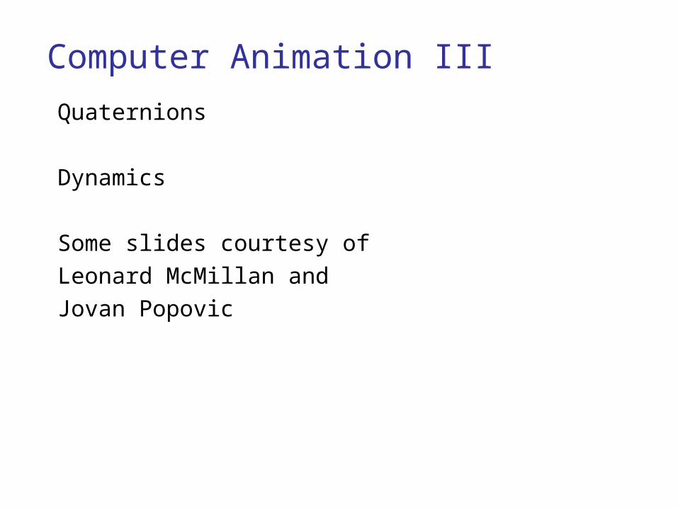
Recap: Euler angles3 angles along 3 axis

Poor interpolation, lock

But used in flight simulation, etc. because natural

http://www.fho-emden.de/~hoffmann/gimbal09082002.pdf

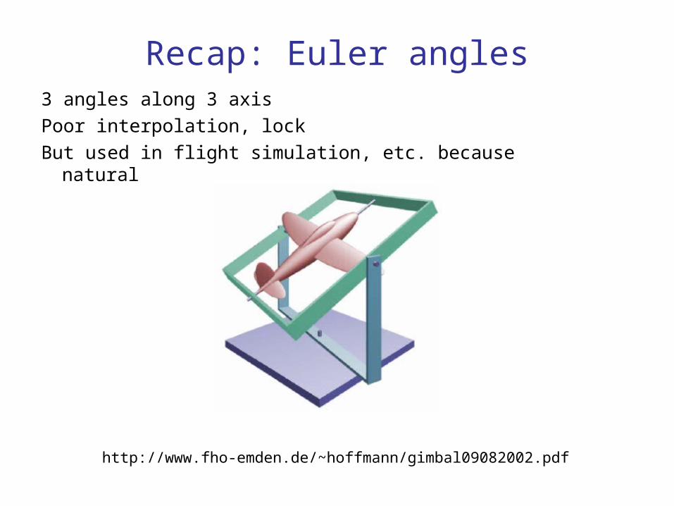
Assignment 5: OpenGLInteractive previsualization

OpenGL API Graphics hardware Jusrsend rendering commands State machine

Solid textures New Material subclass Owns two Material* Chooses between them “Shadertree”

Final project

First brainstorming session on ThursdayGroups of threeProposal due Monday 10/27

A couple of pages Goals Progression

Appointment with staff

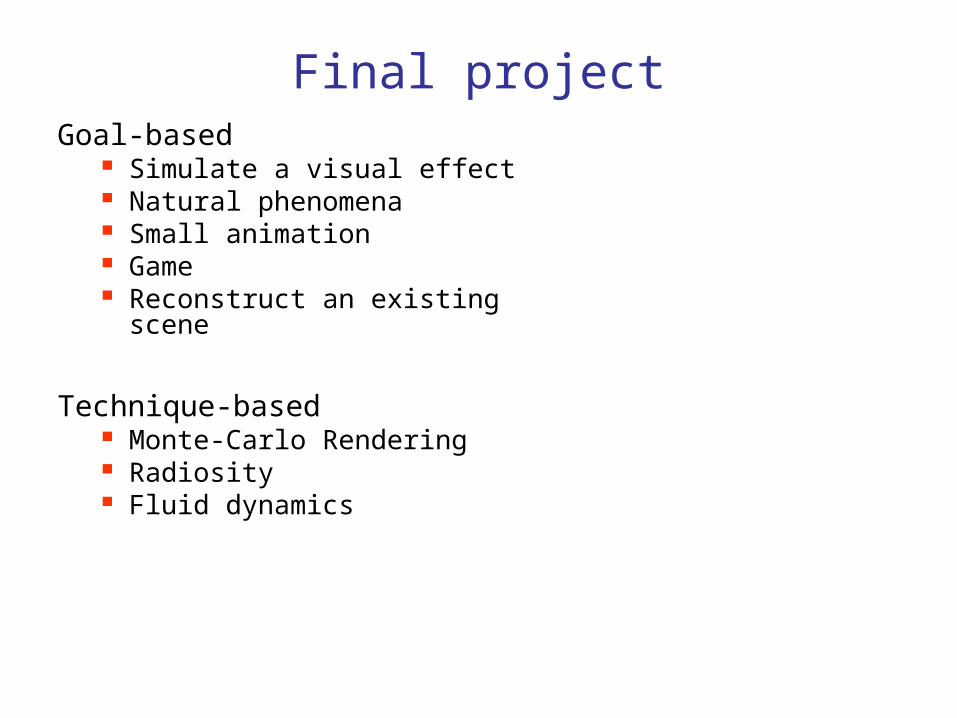
Goal-based Simulate a visual effect Natural phenomena Small animation Game Reconstruct an existing scene

Technique-based Monte-Carlo Rendering Radiosity Fluid dynamics

Final project

OverviewInterpolation of rotations, quaternions

Euler angles

Quaternions

Dynamics

Particles

Rigid body

Deformable objects

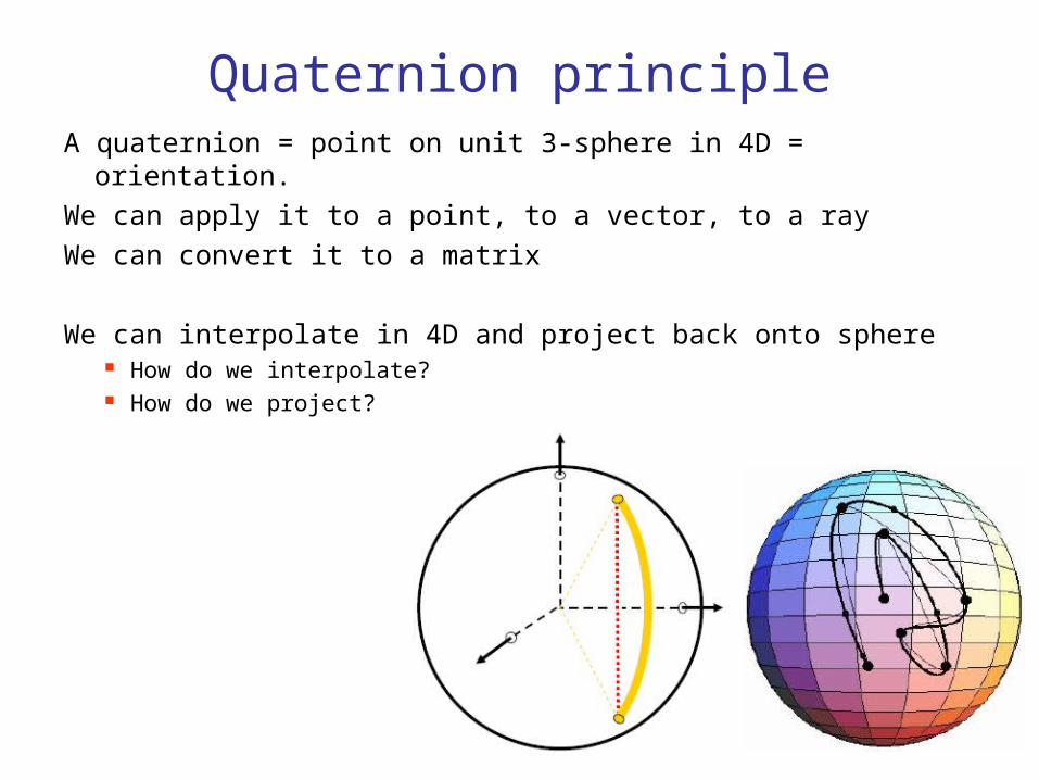
Quaternion principleA quaternion = point on unit 3-sphere in 4D = orientation.

We can apply it to a point, to a vector, to a ray

We can convert it to a matrix

We can interpolate in 4D and project back onto sphere How do we interpolate? How do we project?

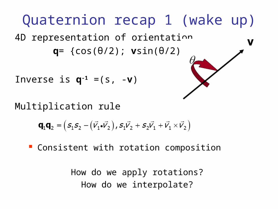
Quaternion recap 1 (wake up)4D representation of orientation

q= {cos(θ/2); vsin(θ/2)}

Inverse is q-1 =(s, -v)

Multiplication rule

Consistent with rotation composition

How do we apply rotations?

How do we interpolate?

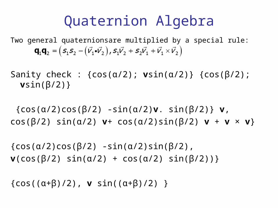
Quaternion AlgebraTwo general quaternionsare multiplied by a special rule:

Sanity check : {cos(α/2); vsin(α/2)} {cos(β/2); vsin(β/2)}

{cos(α/2)cos(β/2) -sin(α/2)v. sin(β/2)} v,

cos(β/2) sin(α/2) v+ cos(α/2)sin(β/2) v + v × v}

{cos(α/2)cos(β/2) -sin(α/2)sin(β/2),

v(cos(β/2) sin(α/2) + cos(α/2) sin(β/2))}

{cos((α+β)/2), v sin((α+β)/2) }

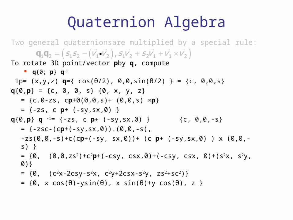
Quaternion AlgebraTwo general quaternionsare multiplied by a special rule:

To rotate 3D point/vector pby q, compute q{0; p} q-1

1p= (x,y,z) q={ cos(θ/2), 0,0,sin(θ/2) } = {c, 0,0,s}

q{0,p} = {c, 0, 0, s} {0, x, y, z}

= {c.0-zs, cp+0(0,0,s)+ (0,0,s) ×p}

= {-zs, c p+ (-sy,sx,0) }

q{0,p} q -1= {-zs, c p+ (-sy,sx,0) } {c, 0,0,-s}

= {-zsc-(cp+(-sy,sx,0)).(0,0,-s),

-zs(0,0,-s)+c(cp+(-sy, sx,0))+ (c p+ (-sy,sx,0) ) x (0,0,-s) }

= {0, (0,0,zs2)+c2p+(-csy, csx,0)+(-csy, csx, 0)+(s2x, s2y, 0)}

= {0, (c2x-2csy-s2x, c2y+2csx-s2y, zs2+sc2)}

= {0, x cos(θ)-ysin(θ), x sin(θ)+y cos(θ), z }

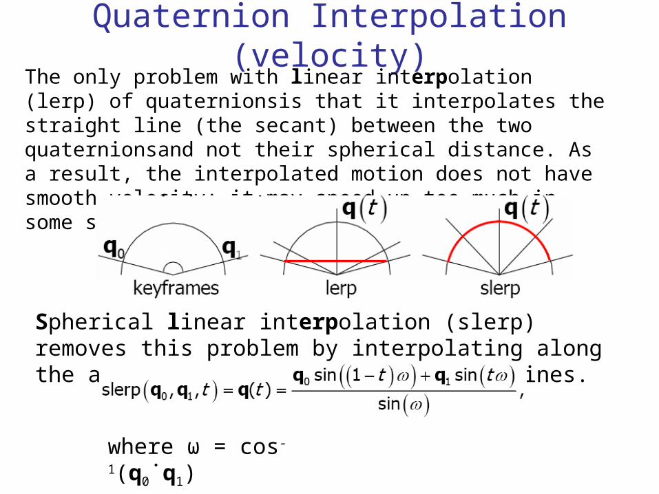
Quaternion Interpolation (velocity)The only problem with linear interpolation (lerp) of quaternionsis that it interpolates the straight line (the secant) between the two quaternionsand not their spherical distance. As a result, the interpolated motion does not have smooth velocity: it may speed up too much in some sections:

Spherical linear interpolation (slerp) removes this problem by interpolating along the arc lines instead of the secant lines.

where ω = cos-1(q0˙q1)

Quaternions

Can also be defined like complex numbers

a+bi+cj+dk

Multiplication rules i2=j2=k2=-1 ij=k=-ji jk=i=-kj ki=j=-ik

…

Fun:Julia Sets in Quaternion spaceMandelbrot set: Zn+1=Zn2+Z0

Julia set Zn+1=Zn2+C

http://aleph0.clarku.edu/~djoyce/julia/explorer.html

Do the same with Quaternions!

Rendered by Skal(Pascal Massimino) http://skal.planet-d.net/

Images removed due to copyright considerations.

See also http://www.chaospro.de/gallery/gallery.php?cat=Anim

Fun:Julia Sets in Quaternion spaceMandelbrot set: Zn+1=Zn2+Z0

Do the same with Quaternions!

Rendered by Skal(Pascal Massimino) http://skal.planet-d.net/

This is 4D, so we need the time dimension as well

Images removed due to copyright considerations.

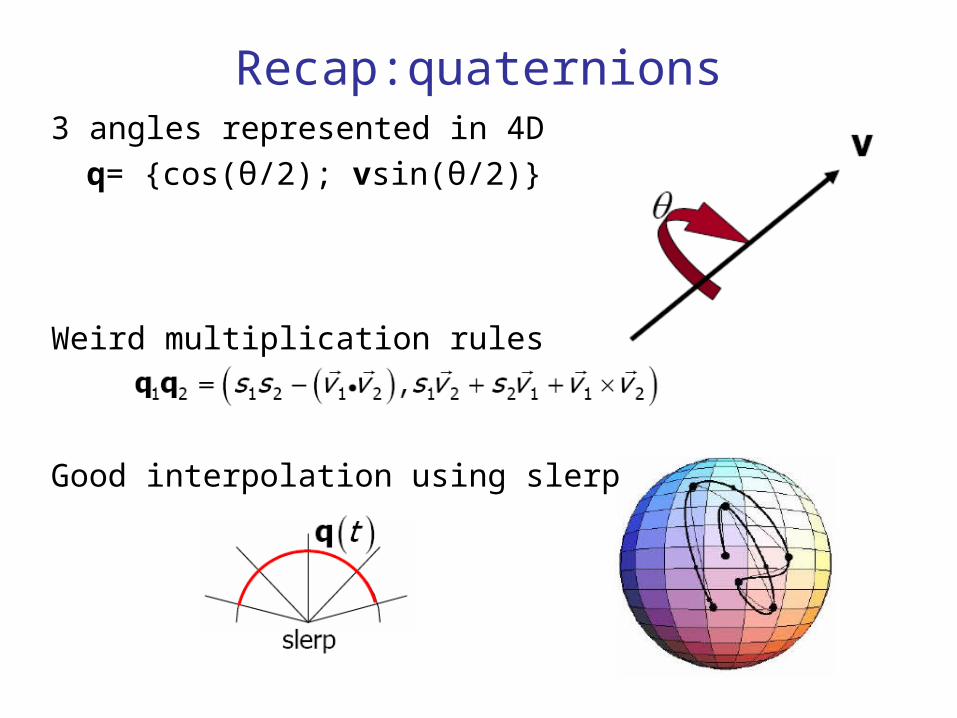
Recap:quaternions3 angles represented in 4D

q= {cos(θ/2); vsin(θ/2)}

Weird multiplication rules

Good interpolation using slerp

OverviewInterpolation of rotations, quaternions

Euler angles

Quaternions

Dynamics

Particles

Rigid body

Deformable objects

Break: movie timePixar For the Bird

NowDynamics

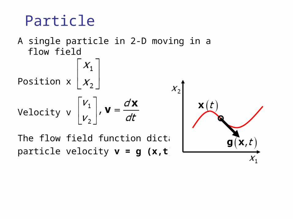
ParticleA single particle in 2-D moving in a flow field

Position x =

Velocity v =

The flow field function dictates

particle velocity v = g (x,t)

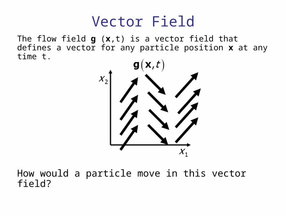
Vector FieldThe flow field g (x,t) is a vector field that defines a vector for any particle position x at any time t.

How would a particle move in this vector field?

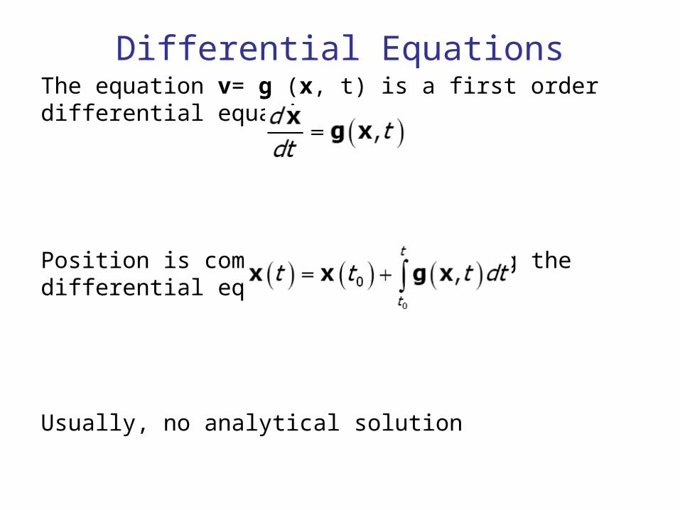
Differential EquationsThe equation v= g (x, t) is a first order differential equation:

Position is computed by integrating the differential equation:

Usually, no analytical solution

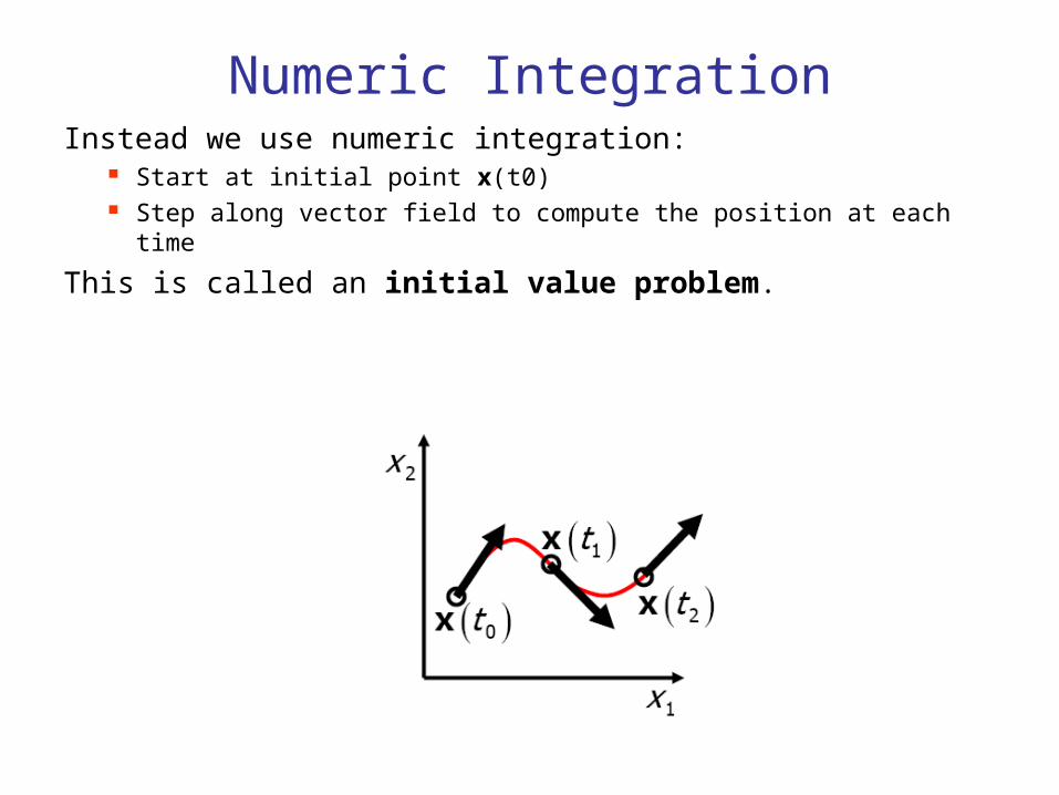
Numeric IntegrationInstead we use numeric integration:

Start at initial point x(t0) Step along vector field to compute the position at each time

This is called an initial value problem.

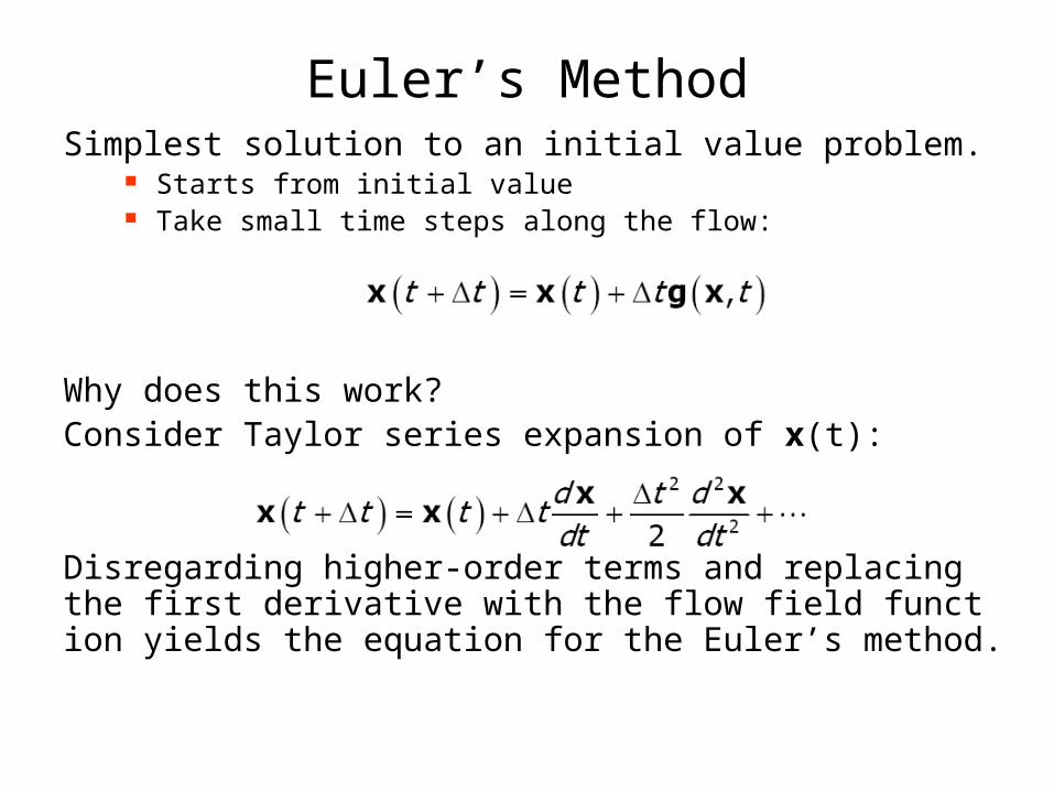
Euler’s MethodSimplest solution to an initial value problem.

Starts from initial value Take small time steps along the flow:

Why does this work?Consider Taylor series expansion of x(t):

Disregarding higher-order terms and replacing the first derivative with the flow field function yields the equation for the Euler’s method.

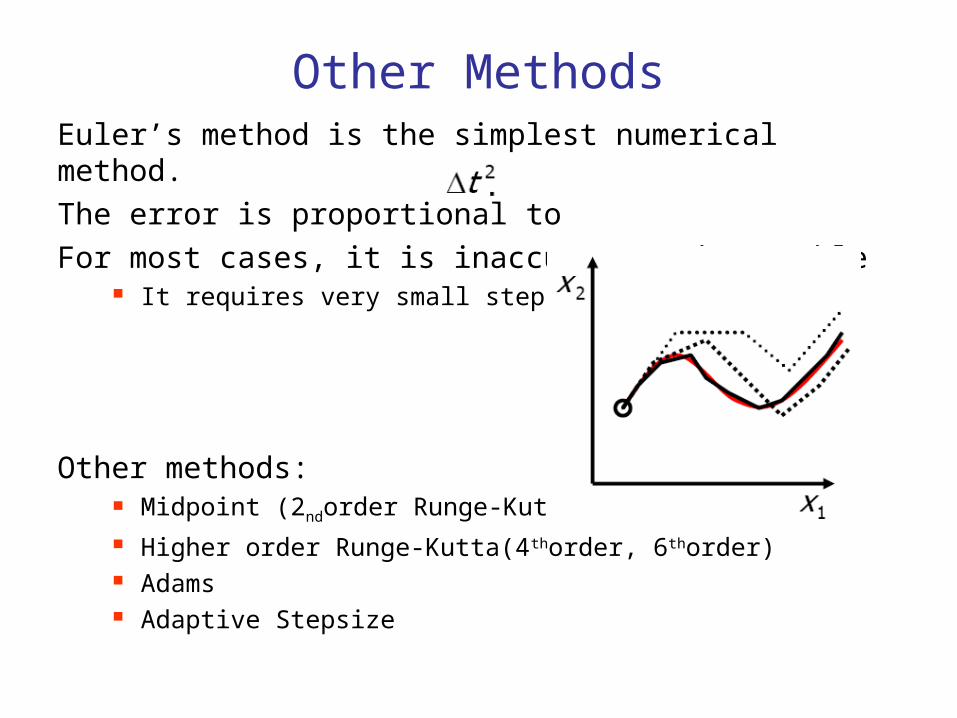
Other MethodsEuler’s method is the simplest numerical method.

The error is proportional to

For most cases, it is inaccurate and unstable It requires very small steps.

Other methods: Midpoint (2ndorder Runge-Kutta) Higher order Runge-Kutta(4thorder, 6thorder) Adams Adaptive Stepsize

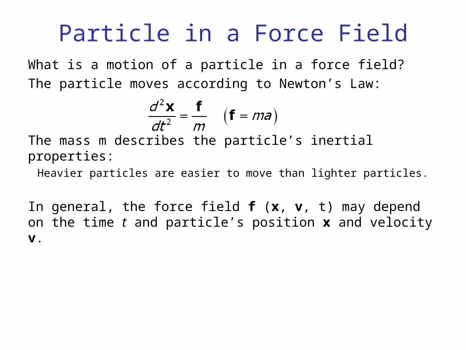
Particle in a Force FieldWhat is a motion of a particle in a force field?

The particle moves according to Newton’s Law:

The mass m describes the particle’s inertial properties:Heavier particles are easier to move than lighter particles.

In general, the force field f (x, v, t) may depend on the time t and particle’s position x and velocity v.

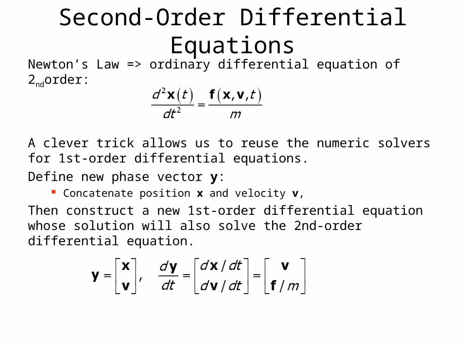
Second-Order Differential EquationsNewton’s Law => ordinary differential equation of 2ndorder:

A clever trick allows us to reuse the numeric solvers for 1st-order differential equations.

Define new phase vector y: Concatenate position x and velocity v,

Then construct a new 1st-order differential equation whose solution will also solve the 2nd-order differential equation.

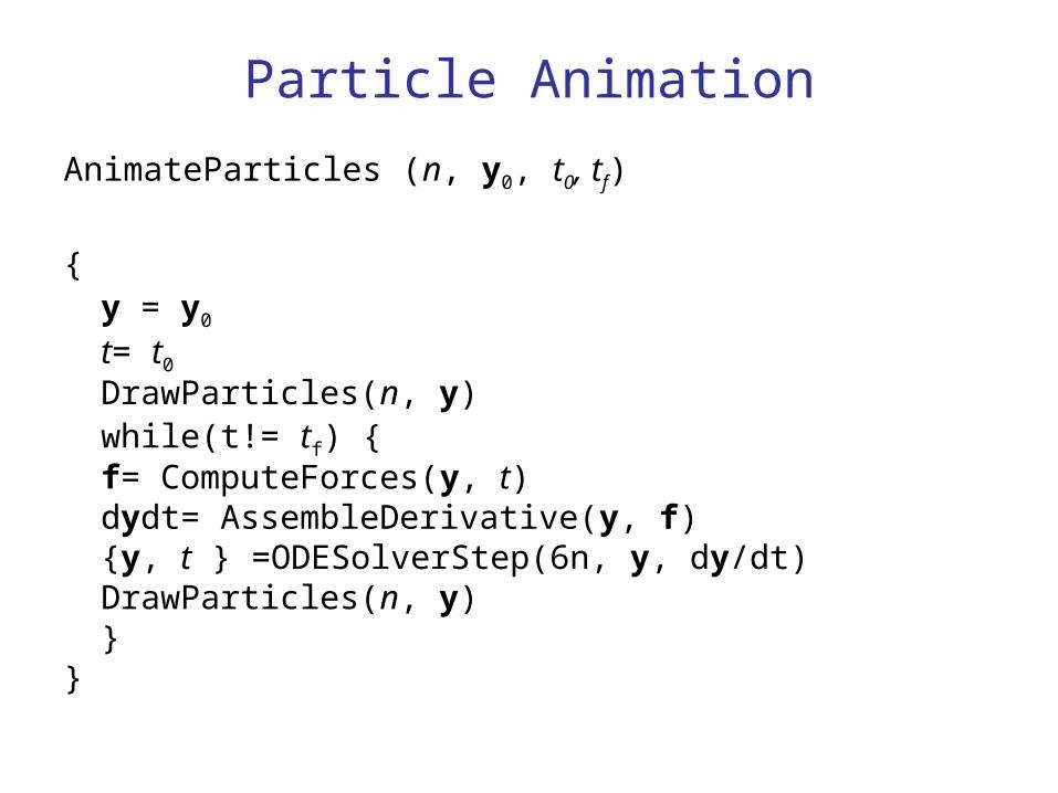
Particle Animation

AnimateParticles (n, y0, t0, tf)

{y = y0

t= t0

DrawParticles(n, y)while(t!= tf) {

f= ComputeForces(y, t)dydt= AssembleDerivative(y, f){y, t } =ODESolverStep(6n, y, dy/dt)DrawParticles(n, y)

}}

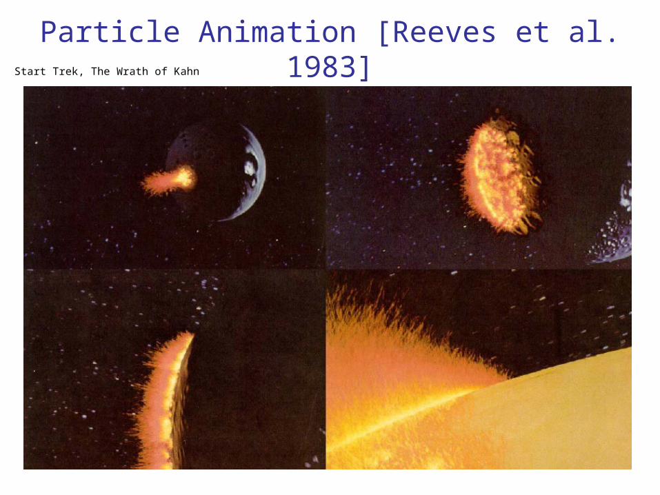
Particle Animation [Reeves et al. 1983]Start Trek, The Wrath of Kahn

OverviewInterpolation of rotations, quaternions

Euler angles

Quaternions

Dynamics

Particles

Rigid body

Deformable objects

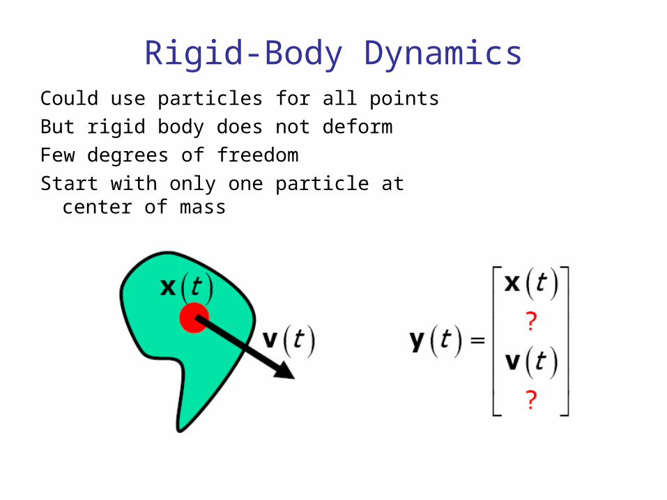
Rigid-Body DynamicsCould use particles for all points

But rigid body does not deform

Few degrees of freedom

Start with only one particle at center of mass

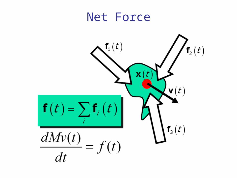
Net Force

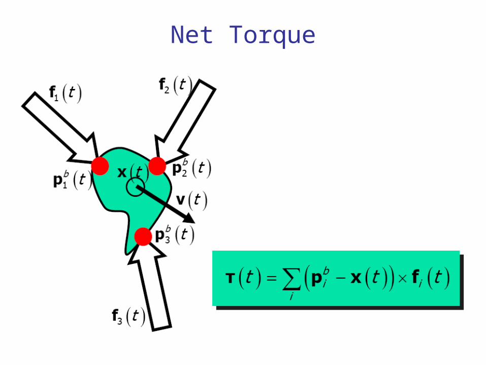
Net Torque

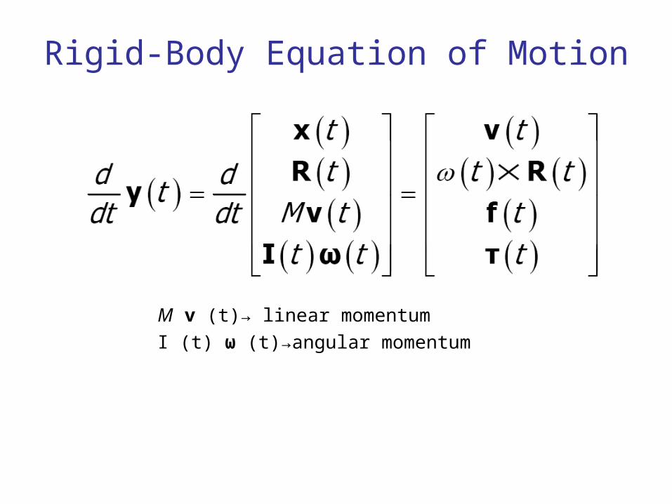
Rigid-Body Equation of Motion

M v (t)→ linear momentum

I (t) ω (t)→angular momentum

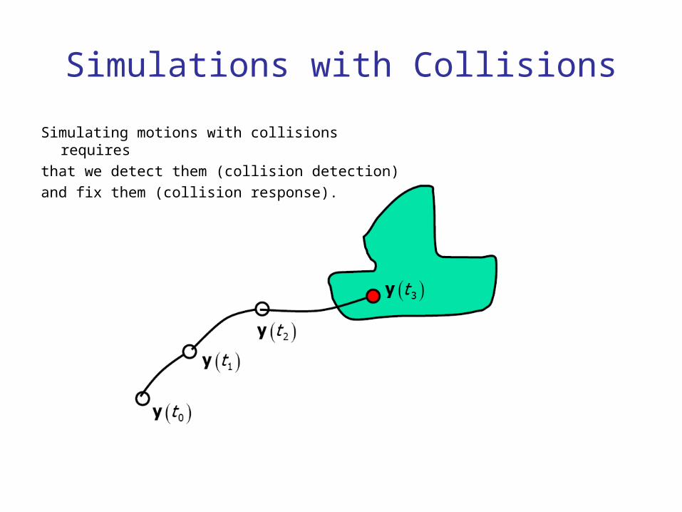
Simulations with Collisions

Simulating motions with collisions requires

that we detect them (collision detection)

and fix them (collision response).

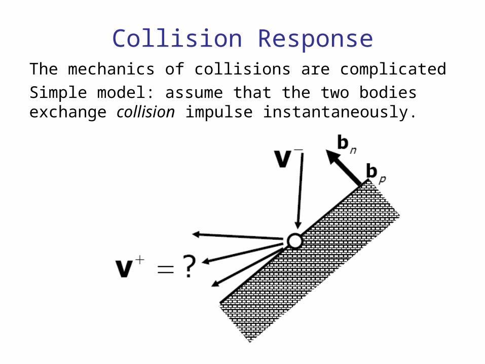
Collision ResponseThe mechanics of collisions are complicated

Simple model: assume that the two bodies exchange collision impulse instantaneously.

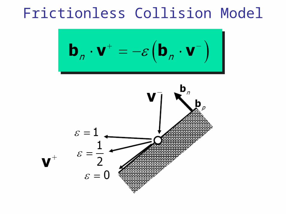
Frictionless Collision Model

OverviewInterpolation of rotations, quaternions

Euler angles

Quaternions

Dynamics

Particles

Rigid body

Deformable objects

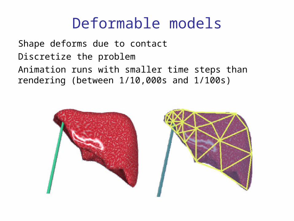
Deformable modelsShape deforms due to contact

Discretize the problem

Animation runs with smaller time steps than rendering (between 1/10,000s and 1/100s)

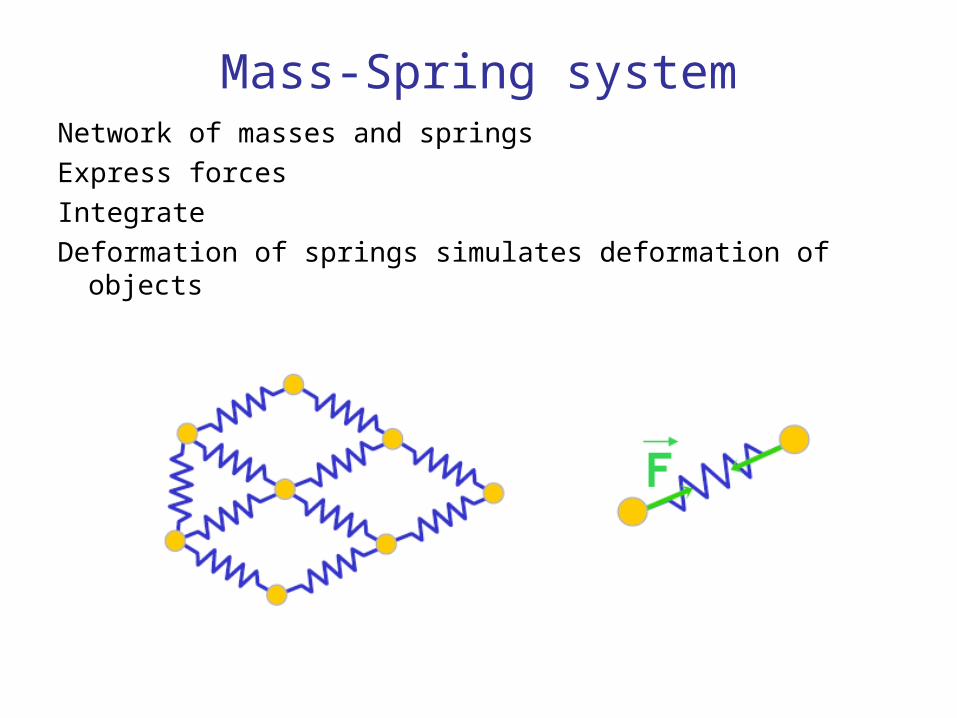
Mass-Spring systemNetwork of masses and springs

Express forces

Integrate

Deformation of springs simulates deformation of objects

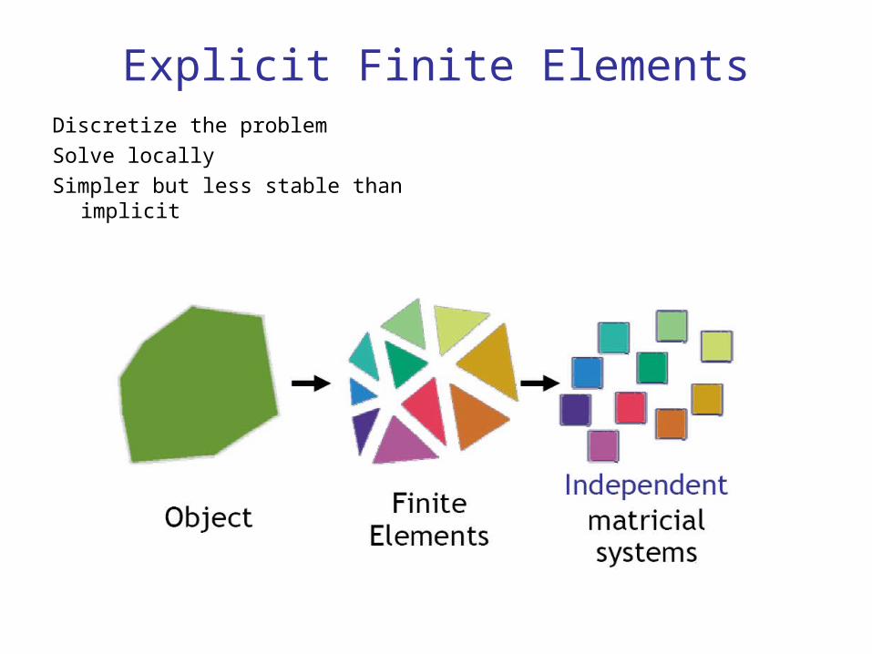
Explicit Finite ElementsDiscretize the problem

Solve locally

Simpler but less stable than implicit

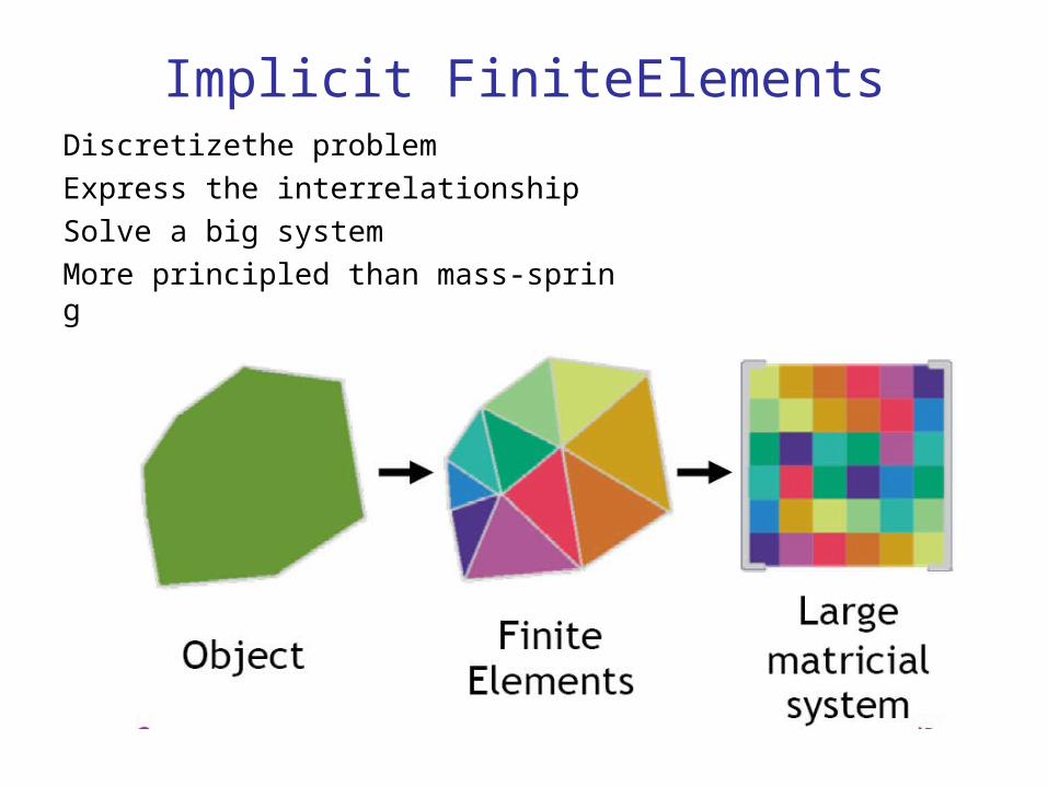
Implicit FiniteElementsDiscretizethe problem

Express the interrelationship

Solve a big system

More principled than mass-spring

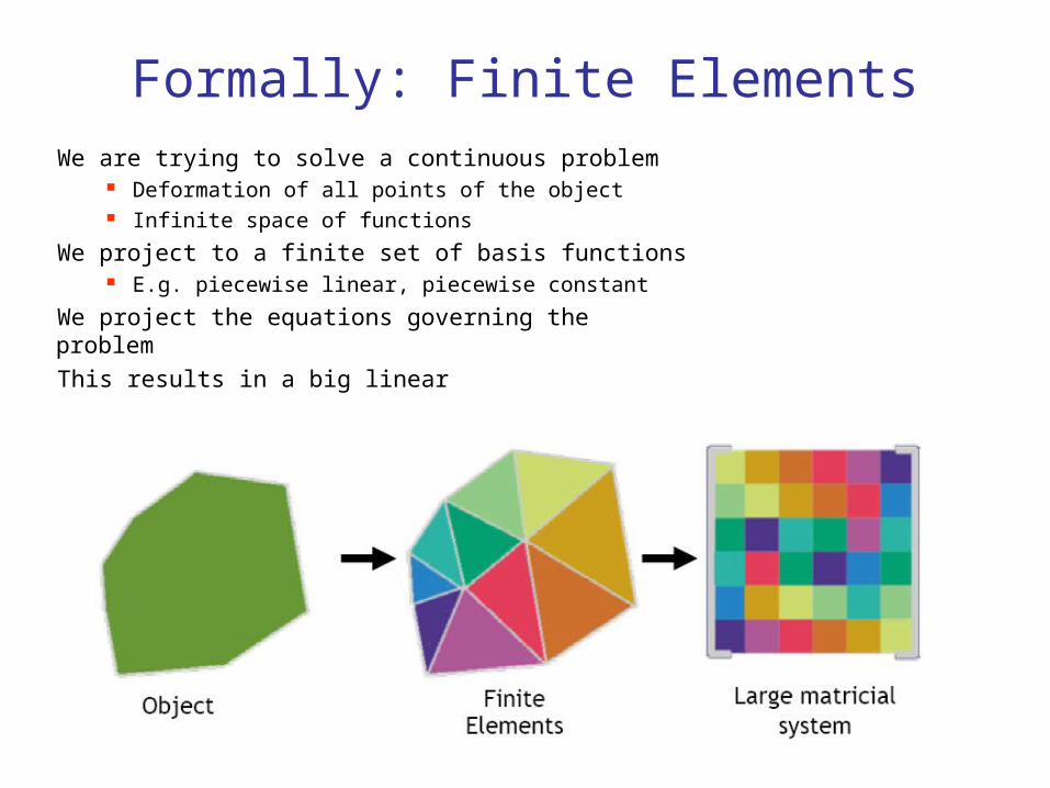
Formally: Finite Elements

We are trying to solve a continuous problem Deformation of all points of the object Infinite space of functions

We project to a finite set of basis functions E.g. piecewise linear, piecewise constant

We project the equations governing the problem

This results in a big linear

Cloth animation Discretize cloth

Write physical equations

Integrate

Collision detection

Image removed due to copyright considerations.

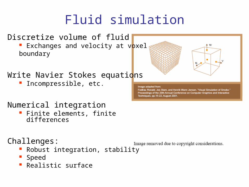
Fluid simulationDiscretize volume of fluid

Exchanges and velocity at voxel boundary

Write Navier Stokes equations Incompressible, etc.

Numerical integration Finite elements, finite differences

Challenges: Robust integration, stability Speed Realistic surface

How do they animate movies?Keyframing mostly

Articulated figures, inverse kinematics

Skinning Complex deformable skin Muscle, skin motion

Hierarchical controls Smile control, eye blinking, etc. Keyframesfor these higher-level controls

A huge time is spent building the 3D models, its skeleton and its controls

Physical simulation for secondary motion Hair, cloths, water Particle systems for “fuzzy” objects

Images removed due to copyright considerations.

Final project

First brainstorming session on ThursdayGroups of threeLarge programming contentProposal due Monday 10/27

A couple of pages Goals Progression

Appointment with staff

Final projectGoal-based

Render some class of object (leaves, flowers, CDs) Natural phenomena (plants, terrains, water) Weathering Small animation of articulated body, explosion, etc. Visualization (explanatory, scientific) Game Reconstruct an existing scene

Technique-based Monte-Carlo Rendering Radiosity Finite elements/differences (fluid, cloth, deformable objects) Display acceleration Model simplification Geometry processing

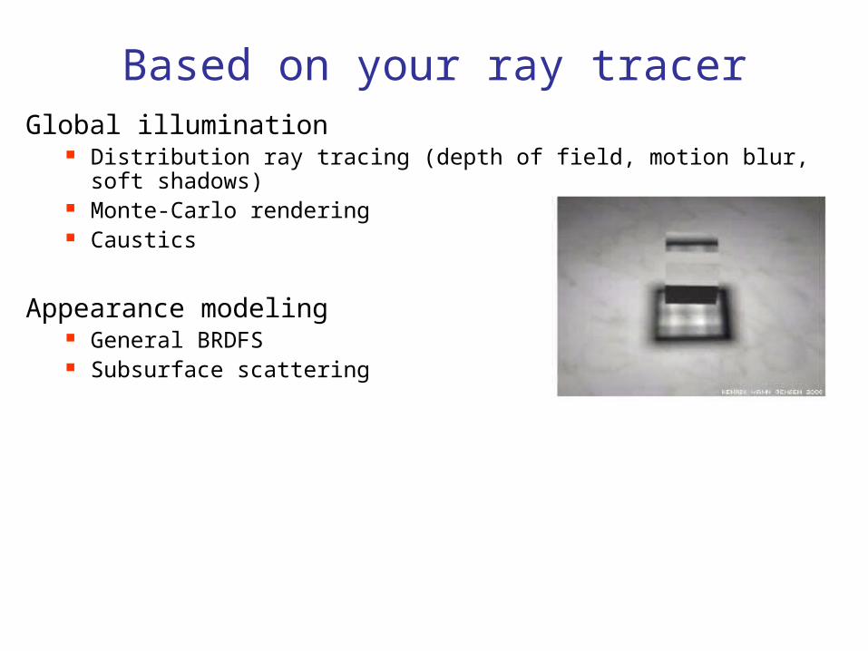
Based on your ray tracerGlobal illumination

Distribution ray tracing (depth of field, motion blur, soft shadows) Monte-Carlo rendering Caustics

Appearance modeling General BRDFS Subsurface scattering