Computer Aided Molecular Design Introduction Our society is faced with challenges that can have a chemical solution. Examples include: bacterial drug resistance, new diseases like AIDS, and agricultural pest control. We also need to develop environmentally benign synthetic methods, for example the use of aqueous solvents and enzymatically catalyzed processes. We are rapidly developing new technologies to help solve these problems, including new receptors such as zeolites and self-assembling systems, and new hosts for guest-host chemistry including crown ethers, cyclodextrins, phase transfer catalysis agents, and supramolecular hosts. Combinatorial synthesis is accelerating the pace of advancement in guest-host chemistry and biochemistry. Each of these areas underscores the need for enhanced uses of molecular mechanics and dynamics, molecular orbital calculations, and chemical information technology. We are part of a large scale international effort to solve the many problems that confront our society. In this effort we have amassed a truly bewildering array of information; we need to learn how to tame this rich resource. A tremendous volume of work has been done, and a bewildering variety of structural motifs have been discovered in nature. Chemical information technology helps us to appreciate the richness and variety of chemical structural complexity. Computer Aided Molecular Design, CAMD, is a combination of computational chemistry and information technology tools that help us to discover new and useful compounds. CAMD touches all areas of chemistry. The discovery of new natural products help us explore structures and functionality that we would never guess are important, for example diepoxides and diacetylides. The vastness of the variety of chemical structures also plays an important role in environmental chemistry and analytical chemistry. Characterizing the biological activity and properties of all the known compounds is impossible. We must develop predictive tools for molecular properties in an environmental setting. Quantitative structure activity relationships (QSAR), Quantitative structure property relationships (QSPR), and 3D-database mining play a central role in this effort. Analytical chemists have developed new chemometric techniques that allow the rapid retrieval and prediction of molecular and biological properties. Multi-variate and artificial intelligence techniques are necessary to efficiently use our wealth of information. This tutorial introduces the use of advanced computational methods in Computer Aided Molecular Design. Computer Aided Molecular Design (CAMD) is a unifying theme that focuses on why we do chemistry and how we decide what to synthesize and study. Chemistry emphasizes the development of predicative tools for understanding structure-function relationships, and the use of CAMD techniques enhances our ability to predict chemical reactivity and design useful compounds.

Computer Aided Molecular Design Phases The goal of Computer Aided Molecular Design (CAMD) is to find ligands that are predicted to interact strongly with a host. Alternatively, this procedure can be reversed to search for hosts that will interact strongly with a given ligand. CAMD is an outgrowth of rational drug design1 where the interactions are protein or DNA binding with substrates. It is clear, however, that CAMD is not restricted to drug design. In fact, much of the current development in chemistry, biochemistry, and biology are coalescing and the divisions in our disciplines are evaporating. As a consequence the tools developed for drug design will become critical for many if not most chemists. In particular, molecular recognition, be it through proteins, DNA, supramolecular chemistry, or self-assembling systems, is a unifying research area. As organic and physical

chemists search for guest-host systems with specificity in binding and catalysis2,3, the basic concepts of molecular field analysis and receptor mapping will be a unifying tool. Rapid advancements in chemistry will increasingly require an interdisciplinary approach; biochemistry, molecular biology, microbiology, cell biology, developmental biology will be key players along with the traditional areas of chemistry. The ready availability of chemical structure databases is playing an important role in enhancing the drug discovery approach and CAMD. These same databases find increasing use in environmental, inorganic, and organic chemistry. Supramolecular and natural products chemistry will demand easy access to information and powerful 3D-searching algorithms. Environmental chemists will need to systematize the reactivity of millions of natuarally occuring and synthetic substances. The basic phases of CAMD can be outlined as shown in Table I1,4. Table I. The Phases in Computer Aided Molecular Design1,4. The "CPU " column compares the relative computation resources needed for each method. Phase Method CPU Determine structure of the ligands or the receptor site: MO calculations + molecular mechanics + molecular dynamics/protein folding +++ homology modeling with database +++ ⇓ Build a model of the receptor site: propose pharmacophore 3D-QSAR or receptor mapping ++ propose steric pocket map surface with a probe + steric model from map (DOCK) + ⇓ Search databases for ligands: 2D-substructure + steric search (docking) ++ 3D-search with pharmacophore +++ ⇓ Dock new ligands to receptor site: molecular mechanics or MO + ⇓ Predict binding constants or activity: 1D, 2D, or 3D-QSAR + free energy perturbation +++ MO transition-state calculations +++ ⇓ Synthesize ligands: reactions database + CAMD can be done in two ways: ligand based or receptor based. Receptor based design starts with a known receptor, such as a protein binding site or supramolecular host. Ligand based

design uses a known set of ligands, but an unknown receptor site. Both approaches are actually very similar. Receptor based CAMD: The first phase is to determine the structure of the binding site using standard structural analysis from X-ray diffraction, NMR, or calculations involving molecular orbital or molecular mechanics and dynamics techniques. In the absence of structural information, homology of the unkown receptor sequence with known structures that have been identified through database searches may be a good starting point. The next phase is to generate a query for database searching. The query is generated by building a simplified model of the receptor site. This model may be based on a pharmacophore, which identifies a few specific interactions that are responsible for the binding (Figure 1.). These interactions include hydrogen bond donors and acceptors, charged groups, and hydrophilic regions such as hydrocarbon side chains, and phenyl groups. The pharmacophore can be generated by visual inspection or by computational techniques. In docking-based searches, the model is based on an analysis of steric interactions over the receptor site. Typically, a solvent accessible surface map is generated and binding pockets are identified on the host surface. More specific interactions can also be specified as in the angiotensin converting enzyme inhibitor pharmacophore5 in Figure 1.

(u)

O(s1)

O(s1) AA

[O,S]

O

3.6 - 4.6 Å3.3 - 4.3 Å

6.8 - 7.8 Å

Figure 1. Pharmacophore for angiotensin converting enzyme (ACE) inhibitors, which describes the spatial arrangement of functional groups necessary for binding to the receptor site of the enzyme5. The dotted bonds are to allow single or double bonds and the A stands for any atom.

The next phase is to search databases for ligands that may bind to the chosen receptor. The 3D-pharmacophore is used in conformationally flexible searches for ligands that match the spatial distribution of the receptor. Alternatively, the receptor pocket can be used with auto-docking to find ligands that avoid close-contacts. The 3D-pharmacophore approach and the binding pocket approach are actually very similar, and queries can be fashioned that incorporate aspects of both approaches. Pharmacophores emphasize a few specific and varied types of interactions, while binding pockets emphasize steric interactions over the entire ligand. The results of the database search may be used directly or modified to produce candidates for further study. These candidates that are inspired by the database search constitute the design element of the procedure. The new ligands or hosts are then assessed for the use at hand. This assesment first involves docking the new molecule and evaluation of the full interaction by molecular orbital calculations or molecular mechanics. Next, calculations are done to predict the binding constant or activity of the compound. Prediction of the binding constants are usually performed using Gibb's free energy perturbation studies based on either Monte Carlo or molecular dynamics simulations. Activity predictions are usually based on QSAR extrapolation. Increasingly these QSAR predictions are based on the 3D-QSAR that was used to generate the pharmacophore in the search stage.

Finally, the candidates are synthesized and tested in the laboratory. Synthetic chemists increasingly use reaction database searches and artificial intelligence tools to design synthetic procedures. Ligand based CAMD: Ligand based design starts with a group of ligands that have known binding constants or biological activities. The first phase is to determine the structure of the ligands using standard structural analysis from X-ray diffraction, NMR, or calculations involving molecular orbital or molecular mechanics and dynamics techniques. The next phase is to generate a query for database searching. The query is generated by building a simplified model of the receptor site. This model is based on a pharmacophore, as in receptor based design. The pharmacophore can be generated by visual inspection or by statistical techniques. One popular statistical technique is 3D-QSAR as represented by the CoMFA approach6. 3D-QSAR maps the steric, charge, and hydrogen bonding interactions into a 3-D grid for each known ligand. These maps are then compared to find features that the active compounds have in common. The map of common features is then converted into a pharmacophore. The next phase is to search databases for new ligands that may also bind to the chosen receptor. 2D-substructure searches based on the known ligands can be used, but such searches have not been very successful. Instead, the 3D-pharmacophore is used in conformationally flexible searches for ligands that match the spatial distribution of the known ligands. The remainder of the phases are identical for ligand and receptor based design. There are many examples of applications of CAMD. Organic chemists are active users of database searching. Physical chemists calculate the free energy of binding or solvation for substances by perturbation techniques. QSAR/QSPR is a major focus in physical organic chemistry, instrumental analysis, and environmental chemistry. Biochemists focus on receptor modeling and substrate docking. In synthetic chemistry reaction databases play an important role. In inorganic chemistry, 3D-database searches are applied to organometallic chemistry and metal complexes.

BIBLIOGRAPHY 1. Y. C. Martin, Computer Assisted Rational Drug Design, in Methods In Enzymology, D. M. J.

Lilley and J. E. Dahlberg, Eds., Academic Press, San Diego,CA, 1991. pp 587-613. 2. J. Rebek, Jr., Molecular Recognition and Biophysical Organic Chemistry, Acc. of Chem. Res.

1990, 23(12), 399-404. 3. Organic 'Tectons' Used To Make Networks With Inorganic Properties. Chem. Eng. News 1995,

January 2, 21-22. 4. L. M. Balbes, Guide to Rational (Computer-Aided) Drug Design, Research Triangle Institute,

Research Triangle Park, NC 27709-2194, from the Ohio Supercomputer Center Computational Chemistry Bulletin board.

5. D. R. Henry, O. F. Güner, Techniques for Searching Databases of Three-Dimensional (3D) Structures with Receptor-Based Queries, Electronic Conference on Trends in Organic Chemistry ECTOC-1, 1995, Paper 44, http://www.ch.ic.ac.uk/ectoc/papers/44/.index.html

6. R. D. Cramer, III, D. E. Patterson, J. D. Bunce, Comparative Molecular Field Analysis (CoMFA). 1. Effect of Shape on Binding of Steroids to Carrier Proteins, J. Am. Chem. Soc., 1988, 110(18), 5959-5967.

QSAR

Introduction The key insight of chemistry is the relationship between molecular structure and molecular function. We use the details of molecular structure to predict the properties of molecules. Medicinal chemistry is a particularly rich example of our use of structure-function relationships. There is a tremendous need to be able to quickly design new drugs for curing human disease. The rapid prediction of the activities of compounds for use as drugs and the discovery of new compounds is an important goal. Quantitative Structure Activity Relationships, or QSAR, allow us to predict the properties of compounds and are a quantitative expression of structure-function relationships. QSAR has been responsible for the rapid development of many new drugs. In QSAR we seek to uncover correlations of biological activity with molecular structure. With Quantitative Structure Property Relationships, QSPR, we extend the same notion to general chemical property prediction and not just biological activity. In either case, the relationship is most often expressed by a linear equation that relates molecular properties, x, y…, to the desired activity, A. For compound i:

Ai = m xi + n yi + o zi + b 1

Where m, n, and o are the linear slopes that express the correlation of the particular molecular property with the activity of the compound, and b is a constant. If only one molecular property is important, for example molecular volume, then Eqn. 1 reduces to the simple form of a straight line, Ai = m xi + b. The slopes and the constant in Eqn. 1 are often calculated using multiple linear regression, MLR, which is analogous with regular linear regression when there is just one independent variable. The molecular properties can be dipole moments, steric energies, molecular volumes, surface areas, free energies of solvation, and a wide variety of others. The molecular properties used in QSAR studies are called descriptors. In Eqn. 1 we show only three descriptors. In a typical QSAR study, scores of descriptors are often used. However, in the final QSAR equation we seek to find the smallest number of descriptors that can adequately model the activity of the compounds in the study. For the general case with p descriptors, xj :

Ai = ∑j=1

pmj xj + b 2

gives the more general QSAR equation form. Activities An example of a QSAR study is the isonarcotic activity of esters, alcohols, ketones, and ethers with tadpoles, Table 1. In this study various organic compounds were added to water with swimming tadpoles. The swimming speed of the tadpoles was observed and the amount of the compound that was necessary to slow the tadpoles swimming was determined. A very effective compound has a very low concentration for the production of the desired effect. In QSAR studies we often like to have the more effective compounds have a higher “activity,” not a lower. Therefore, it is very common to transform the concentration for a desired effect, C, to an activity by:

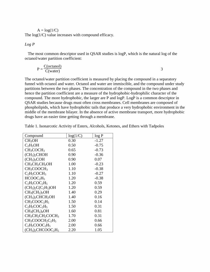
A = log(1/C)

The log(1/C) value increases with compound efficacy. Log P The most common descriptor used in QSAR studies is logP, which is the natural log of the octanol/water partition coefficient:

P = C(octanol)C(water) 3

The octanol/water partition coefficient is measured by placing the compound in a separatory funnel with octanol and water. Octanol and water are immiscible, and the compound under study partitions between the two phases. The concentration of the compound in the two phases and hence the partition coefficient are a measure of the hydrophobic-hydrophilic character of the compound. The more hydrophobic, the larger are P and logP. LogP is a common descriptor in QSAR studies because drugs must often cross membranes. Cell membranes are composed of phospholipids, which have hydrophobic tails that produce a very hydrophobic environment in the middle of the membrane bilayer. In the absence of active membrane transport, more hydrophobic drugs have an easier time getting through a membrane. Table 1. Isonarcotic Activity of Esters, Alcohols, Ketones, and Ethers with Tadpoles Compound log(1/C) log P CH3OH 0.30 -1.27 C2H5OH 0.50 -0.75 CH3COCH3 0.65 -0.73 (CH3)2CHOH 0.90 -0.36 (CH3)3COH 0.90 0.07 CH3CH2CH2OH 1.00 -0.23 CH3COOCH3 1.10 -0.38 C2H5COCH3 1.10 -0.27 HCOOC2H5 1.20 -0.38 C2H5COC2H5 1.20 0.59 (CH3)2C(C2H5)OH 1.20 0.59 CH3(CH2)3OH 1.40 0.29 (CH3)2CHCH2OH 1.40 0.16 CH3COOC2H5 1.50 0.14 C2H5COC2H5 1.50 0.31 CH3(CH2)4OH 1.60 0.81 CH3CH2CH2COCH3 1.70 0.31 CH3COOCH2C2H5 2.00 0.66 C2H5COOC2H5 2.00 0.66 (CH3)2CHCOOC2H5 2.20 1.05

0

0.5

1

1.5

2

2.5

-1.5 -1 -0.5 0 0.5 1 1.5

log P

log

1/C

Figure 1. Isonarcotic Activity of Esters, Alcohols, Ketones, and Ethers with Tadpoles

When the data in Table 1 is submitted to least squares linear regression, Figure 1, the resulting QSAR equation is:

log(1/C) = 0.731 log P + 1.22 n = 20 r = 0.881 4 The data for 20 compounds is reasonably correlated with a regression coefficient of 0.881, indicating a moderately good fit. In this study only one descriptor is necessary to build an adequate model of the structure-function relationships, but often many descriptors are needed. Addition of other descriptors would certainly improve the fit for this case also. Correlation does not imply Causation It is always important for studies of this type to underscore the difference between correlation and causation. We shouldn’t read too much into QSAR equations. A good QSAR correlation does not mean that the particular descriptor “causes” the efficient action of the drug. For example, the correlation of isonarcotic activity to log P does not necessarily mean that getting the drug across the membrane barrier is the important step for biological activity. Instead, the log P dependence may be caused by more efficient blood transport, more efficient interactions with nerve receptors, or a myriad of other interactions both major and minor that add up to the net effect. The lack of evidence on causation, or in other words the mechanism of action, may be disappointing at first. However, the goal of QSAR is to predict activity, and that goal is often admirably filled. Information on the various mechanisms leading to biological activity must be done through additional, careful experimentation.

The History of QSAR The genesis of QSAR is from physical organic chemistry and linear free energy relationships. The first such studies were done by L. P. Hammett. His goal was to uncover the effects of electronic structure on organic reactivity. A short discussion of his work will be instructive as we start to understand the foundations of QSAR. Hammett’s first studies were to understand the effect of electron withdrawing and donating groups on the pKa’s of substituted benzoic acids, Table 2. Hammett first wanted to develop a descriptor that described inductive substituent effects. He compared the log Ka for a variety of substituted benzoic acids with the log KaH for unsubstitued benzoic acid to define the σ substutuent constant.

σ = log Ka - log KaH 5 Table 2 lists the Hammett constants for meta and para substituents. He then postulated that other properties, other than acidity, would be likewise effected by the same substituent effects, and that these other properties would follow the relationship

log (property) = ρ σ + cst 6

In other words, the expected function was a linear relationship with the σ inductive constant. Hammett showed that a wide variety of organic thermodynamic and kinetic properties followed Eqn. 6. Table 2. Hammett substituent constants for inductive effects.

Why did Hammett choose to work with log functions? He took his inspiration from the relationship between Gibb’s Free Energy and the equilibrium constant for a reaction,

∆rG = - RT ln Keq 7 In other words, the energetics of reactions is related to concentration measurements by logarithmic relationships. Eqn. 6 is just one example of many such relationships used by

OOH

R1

Group σp σm

-NH2 -0.57 -0.09 -OH -0.38 0.13 -OCH3 -0.28 0.10 -CH3 -0.14 -0.06 -H 0 0 -F 0.15 0.34 -Cl 0.24 0.37 -COOH 0.44 0.35 -CN 0.70 0.62 -NO2 0.81 0.71

Hammett and many other organic chemists. All such equations are called linear free energy relationships, or LFERs. In this context, QSAR is just an extension of LFERs into the world of biological structure-function relationships. Corwin Hansch at Pomona College is responsible for the early development of QSAR, and has compiled an extensive database of thousands of QSAR equations that are extracted from the literature (http://clogp.pomona.edu/). Hammett σ constants are commonly used as descriptors in QSAR. An example of using Hammett σ constants in QSAR is work on sulfa drugs. The activity of different sulfa drugs was tested on E. coli. Linear regression yielded the QSAR equation

log 1/C = 1.05 σ - 1.28 8

Therefore, even though Hammett’s σ constants were derived from acidity data of benzoic acids, the same inductive effects correlate well with the activity of a common class of antibiotics. The important point of Eqn. 8 is that we now have a hint of how to design a better drug: choose a substituent with a larger σ or use multiple substitutions.

Descriptors A common issue in chemistry is how to describe molecules and their properties. Quantitative measures are necessary for QSAR studies. Molecular descriptors fall into three general categories, steric, hydrophobic, and electronic. Molecular volumes, surface areas, and bond connectivity indices are steric in nature. Molecular volume and surface area are calculated by placing a sphere on each atom with the radius given by the Van der Waals radius of the atom. The steric energy from molecular mechanics calculations is quite useful. Another useful steric descriptor is the number of rotatable bonds. As the number of rotatable bonds increases, the molecule becomes more flexible and more adaptable for efficient interaction with hosts. Electronic descriptors include dipole moments, polarizability, and electronic energies. These values are available from molecular orbital calculations. The HOMO-LUMO band gap energy is often used for QSAR. Hammett substitutent constants are also examples of electronic descriptors. The number of hydrogen bond donors and acceptors and measures of the pi-pi donor-acceptor ability of molecules are also useful. Log P is an example of a hydrophobic molecular descriptor. Molecular surface areas can also be divided into hydrophobic and hydrophilic parts. For these surface area descriptors, Van der Waal’s spheres are again used, but the hydrophilic surface area is the sum over all electronegative surface atoms (N, O, S) and H’s in polar bonds(e.g. O-H, N-H, S-H). The hydrophobic surface area is the sum over all non-electronegative atoms and H atoms that are in non-polar bonds ( e.g. C-H bonds). Log P is also the basis for other descriptors. π: Lipophilic Character

O

S

NH2

O

NH X

The lipophilic character, π, of a substitutent is defined as π = log P – log PH 9 where log P is the value for the substituted benzoic acid and log PH is the value for unsubstituted benzoic acid. π is a commonly used descriptor for hydrophobic or lipophilic effects. The concentration of substituted penicillins curing 50% of mice infected with S. aureus was determined and the activity correlated well with π:

N

SNH

O

OO

OH

Y

X

log 1/C = -0.46 π + 4.85 n=20 r=0.91 10 Free Energies of Desolvation Solvation plays a very important role in molecular interactions. Log P is directly related to solvation. P is the equilibrium constant for the process:

M (aq) –> M (octanol) ∆PG = -RT ln P = -RT 2.303 log P 11

and ∆PG is the corresponding Gibb’s Free energy change for the process. The partitioniong process can be broken into two separate reactions, the desolvation from water

M (aq) –> M (g) ∆desolG(aq) 12

and the desolvation from octanol:

M (octanol) –> M (g) ∆desolG(octanol) 13

The Free Energy of desolvation in water, ∆desolG(aq), is often written as Fh2o or Esol and the Free Energy of desolvation in octanol, ∆desolG(octanol), is often written as Foct. Eqn. 11 for the full partitioning is equivalent to Eqn. 12 – Eqn 11, and the energy effects are

∆PG = ∆desolG(aq) – ∆desolG(octanol) or 14 ∆PG = Fh2o – Foct

Log P can then be calculated using Eqn. 11:

log P = – (1/2.303RT) Fh2o – Foct 15

Note that 1/2.303RT = – 0.735 kcal-1 mol. Therefore, if experimental values for log P are not known, log P can be estimated from free energies. Free energies of desolvation have been studied extensively. A group additive properties approach has been taken to estimating these free energies. Group additive property, GAP,

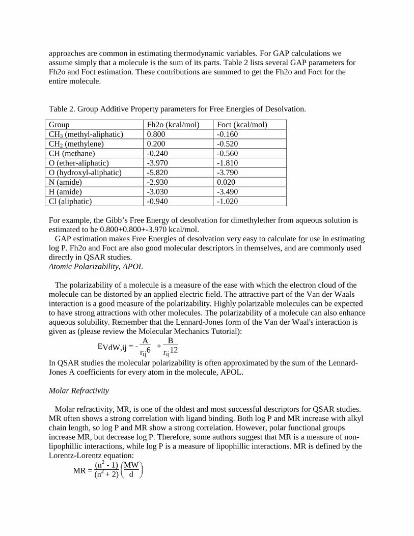
approaches are common in estimating thermodynamic variables. For GAP calculations we assume simply that a molecule is the sum of its parts. Table 2 lists several GAP parameters for Fh2o and Foct estimation. These contributions are summed to get the Fh2o and Foct for the entire molecule. Table 2. Group Additive Property parameters for Free Energies of Desolvation.

Group Fh2o (kcal/mol) Foct (kcal/mol) CH3 (methyl-aliphatic) 0.800 -0.160 CH2 (methylene) 0.200 -0.520 CH (methane) -0.240 -0.560 O (ether-aliphatic) -3.970 -1.810 O (hydroxyl-aliphatic) -5.820 -3.790 N (amide) -2.930 0.020 H (amide) -3.030 -3.490 Cl (aliphatic) -0.940 -1.020 For example, the Gibb’s Free Energy of desolvation for dimethylether from aqueous solution is estimated to be 0.800+0.800+-3.970 kcal/mol. GAP estimation makes Free Energies of desolvation very easy to calculate for use in estimating log P. Fh2o and Foct are also good molecular descriptors in themselves, and are commonly used directly in QSAR studies. Atomic Polarizability, APOL The polarizability of a molecule is a measure of the ease with which the electron cloud of the molecule can be distorted by an applied electric field. The attractive part of the Van der Waals interaction is a good measure of the polarizability. Highly polarizable molecules can be expected to have strong attractions with other molecules. The polarizability of a molecule can also enhance aqueous solubility. Remember that the Lennard-Jones form of the Van der Waal's interaction is given as (please review the Molecular Mechanics Tutorial):

EVdW,ij = - A

rij6 +

B

rij12

In QSAR studies the molecular polarizability is often approximated by the sum of the Lennard-Jones A coefficients for every atom in the molecule, APOL. Molar Refractivity Molar refractivity, MR, is one of the oldest and most successful descriptors for QSAR studies. MR often shows a strong correlation with ligand binding. Both log P and MR increase with alkyl chain length, so log P and MR show a strong correlation. However, polar functional groups increase MR, but decrease log P. Therefore, some authors suggest that MR is a measure of non-lipophillic interactions, while log P is a measure of lipophillic interactions. MR is defined by the Lorentz-Lorentz equation:

MR = (n2 - 1)(n2 + 2)

MW

d

Where n is the index of refraction, MW is the molecular weight, and d is the density. MR has a strong correlation with the molecular polarizability. When experimental values are not available, MR is also often apporximated from group-additive constants like many other descriptors.

Summary Physical chemistry has often been called “the elegant science of drawing straight lines.” This tongue-in-cheek saying is never truer as in QSAR. In one sense there is nothing magical about searching for log-linear relationships in biological activity. The QSAR results don’t really explain anything. QSAR equations just point to correlations. On the other hand, QSAR is a very important and routine method for many areas of chemistry. QSAR is best appreciated as a guide for our chemical intuition. QSAR models guide us to what to synthesize next in our search for more effective solutions to our problems.

Design and QSAR

One goal of QSAR to decide what molecules to synthesize next. It is sometimes difficult to decide how to make changes to the lead compounds based on the QSAR coefficients and descriptors. Some cases are easy. If molecular weight has a strong positive correlation with activity, simply increasing the molar mass by adding some heavy substituents like Br or t-butyl may work well. If surface area is an important component then adding a benzene ring might be useful. If log P has a strong positive correlation, then adding a “greasy” side chain like an n-butyl or cyclohexane ring would increase lipid solubility. One strategy of medicinal chemists is the use of the series: methyl, ethyl, propyl, isopropyl, butyl, t-butyl for substitutions at various spots in the molecule. For the series methyl, ethyl, propyl, and t-butyl, molecular weight, surface area, molar refractivity, and log P (π) increase, Table 1. The volume varies as: methyl, ethyl, propyl ~ iso-propyl, n-butyl, t-butyl. Halogens are also commonly substituted for hydrogen. Fluorine has similar hydrophobic character to hydrogen, but a larger surface area. Table 1. Substituent Parameters for Common Substituents.1

Substituent Volume (SA) MR π Rot Bonds -H 1.48 0.10 0 (reference) 0 -CH3 18.78 0.57 0.56 0 -CH2CH3 35.35 1.03 1.02 1 -CH2CH2CH3 51.99 1.5 1.55 2 -CH(CH3)2 51.33 1.5 1.53 1 -CH2CH2CH2CH3 68.63 1.96 2.13 3 -C(CH3)3 86.99 1.96 1.98 1 -C6H5 72.20 2.54 1.96 1 -F 7.05 0.10 0.14 0 -Cl 15.85 0.60 0.71 0 Both log P and MR increase with alkyl chain length, so log P, π, and MR show a strong correlation. However, polar functional groups increase MR, but decrease log P. MR, however, is insensitive to chain branching. The number of rotatable bonds increases ligand flexibility to adapt to a particular binding pocket. Linear alkyl chains have more rotatable bonds than branched alkyl chains. If you want to design in some shape flexibility, use straight chain substituents. The comparisons in Figure 1 may also be helpful for getting a better feel for log P. LogP increases with alkyl chain length and decreases with chain branching. In other words, branched hydrocarbon chains are more soluble in water than linear chains. Molecules with charged functional groups, like quaternary amines and carboxylates are the most soluble and therefore have very negative logP. Alcohols are more soluble in water than corresponding amines, that is, alcohols have lower log P.

Figure 1. Correlation of log P with structure for alcohols and amines. Calculations by CLOGP program, http://www.daylight.com/release/index.html. The concept of biological isosteres is also useful when designing ligands. Functional groups that have similar properties are called isosteres. The similarity can be based on size, electronic properties, or chemical function. For example, isosteres for the carboxyl group are given in Table 2. For the carboxyl isosteres the similarity is based on chemical function, specifically, acid-base characteristics. Size, molar refractivity and log P (π) have a large variation. The tetrazole group, which is listed third in the table, is one of the most widely used isosteres. Table 2 Bioisosteres for the carboxyl group1 with typical pKa values for aryl compounds.2

Substituent pKa π MR -COOH 4.2 -0.32 6.9 -COO- -4.36 6.0

N NN

NH

(tetrazols)

4.5 -0.48 15.6

N NN

N

-3.55 14.6

-SO3- (sulfonates) -4.76 ~10

-SO2NH2 (sulfonamides) 10 -1.82 12.3 -P(O)(OH)2 (phosphonic acids) 1.42 -1.59 12.6 Sulfonates are completely ionized at physiological pH, so they are a good substitute for carboxyl if the anion form of the drug is the active form. Sulfonamides are very weak acids; therefore they are good isosteres for carboxyl groups only if the active form is protonated. The order of hydrophobicity for the anions is –SO3

- < -COO- < tetrazoyl. If the anionic form of the drug is the bound form and QSAR shows hydrophibic character is better, then tetrazoyl substitution for carboxyl is a good suggestion. Bioisoteres for the carbonyl group include amides, sulfoxides, sulfones, and sulfonamides. Isosteres for the hydroxyl group include many of the same functional groups, Table 3. The activity of a particular functional group depends on the target protein. For some binding sites sulfonamides may be good isosteres for carboxyls. For other binding sites sulfonamides might be

lloogg PP

hydrophillic

hydrophobic

ethanol -.75

pentanol 0.81

isopropanol -0.36 n-propanol -0.23

benzene 2.13

methanol -1.27

tetraethylammonium iodide -2.82 phenylalanine -1.38

alanine -2.85

pyridine 0.64

imidazole -0.08

diethylamine 0.45

butylamine 0.85

good isosteres for hydroxyls. In other words, not all isosteric functional groups are interchangeable for every problem. The actual activity of a given ligand always needs to measured in the laboratory. When looking at a set of known active compounds for a given pharmaceutical target, the student might wonder how anyone came up with the substitutions that are used. The isosteres we have discussed, however, should be very helpful when looking at a set of active compounds. Using these ideas you can follow the logic of the medicinal chemists who have designed the drugs that are in use today. Example analgesics are shown in Figure 2. Table 3. Possible bioisosteres for OH.1 Substituent σp π MR -OH -0.37 -0.67 2.9

NH

CH3

O

(amides)

0.00 -0.97 14.9

NH

SO

OCH3

(sulfonamides)

0.03 -1.18 18.2

-CH2OH 0.00 -1.03 0.72

NH

NH2

O

(ureas)

-0.24 -1.30 1.37

NH

C N

(aminonitrile)

0.06 -0.26 1.01

N

O

OH

N

O

O

O N

O

acetaminaphen phenacetin butacetin (Tromal) Figure 2. Analgesics showing ethyl and t-butyl substitution and a carbonyl or carboxyl isostere. References 1. Hansch, C, Leo, A., Exploring QSAR, Fundamentals and Applications in Chemistry and Biology, American Chemical Society, Washington, DC, 1995. Chapt. 13. 2. Franz, R. G., “Comparison of pKa and Log P Values of Some Carboxylic and Phosphonic Acids: Synthesis and Measurement,” AAPS PharmSci., 2001, 3(2), article 10.

QSAR of Antitumor Activity in Aziridinyl Benzoquinones Quinones are a general class of compounds with the structure in Figure 1a. These compounds are thought to undergo reduction in cells to form 0-quinone methides that are strong alkylating agents1. Alkylating agents attach alkyl groups to the bases in DNA. A series of 2,5-bis(1-aziridinyl)-p-benzoquinones have been tested against lymphoid leukemia in mice2. The data in our study table are for chronic treatment with daily injection for 12 days and are given as the log(1/MED), where MED is the minimum effective dose that gives a 40% increase in life span. The general formula for the aziridinyl benzoquinones is shown in Figure 1b.

Figure 1a. Benzoguinone Figure 1b. 2,5-bis(1-aziridinyl)-p-benzoquinones In this exercise we wish to understand the effect of different R groups on the anti-cancer activity of this group of compounds. Procedure 1. Login in to the "cerius" account. Pull down the Toolchest Desktop menu and select "Unix Shell". In the blue winterm window type "cerius2". 2. In the Visualizer window in the upper right-hand side of the screen pull down the File menu and choose "Load Session". (Note: "Load Model" loads a single molecule, while "Load Session" loads all the molecules in a study). Double click on the benzo/ directory and then click on "benzoquin.mss" entry. Click on the "Load" button. (Note: entries in the file list that have a trailing "/" are directories.) All 28 of the molecules in this study will be loaded. 3. In the Models list (under the big Cerius2 header) scroll up to the top of the list and click on the red diamond next to the first entry. The first entry will be displayed in the larger window on the structure display area. The first entry has R1=CH3 and R2=CH(OCH3)CH2OH and is the most active compound. 4. Locate the R groups and verify their identity. The mouse buttons are mapped as: Left: selection Middle: x-y translation Right: rotation Shift Middle: zoom Shift Right: Atom Information

O

O

N

N

O

O

R1

R2

5. These molecules have already been molecular mechanics minimized. However, we need to make sure that energetic calculations are done with the Merck Force Field, or MMFF. Pull down the tan Card Deck menu above the card stack window in the upper-right corner of the screen and choose "MMFF". On the MMFF card click on "Run". Make sure the box is checked next to "Use MMFF for Energetic Calculations". Click on the |><| go-away box in the upper right-hand corner of the Run dialog box. 6. Pull down the tan Card Deck menu and choose "Drug Discovery". Make sure the QSAR card is on top of the deck. If it is not, click on the cream colored border labeled QSAR. 7. Click on the "Show Study Table" line. The 18 molecules and their activities will be listed in the study table. First we need to specify that the Activity column is to be used as the dependent, or Y variable: to do this click on the Activity label at the top of the data column and then click on

the |Y icon button along the top row of the Study Table window. Now we need to have the

molecular descriptors added to the table: to do this pull down the Descriptors menu in the STudy Table menu bar and choose "Add Default". 8. Some of the default descriptors are not useful for this study and need to be deleted from the study table. We will just need the magnitude values for the dipole moment. Click on the column heading Dipol-X and then shift-click on Dipol-Z. Click on the Delete Rows/Columns icon

button, ↓ . Repeat the same process with PMI-MAG, PMI-X, PMI-Y, and PMI-Z. PMI is

the principal moment of inertia. 9. We also need to add some descriptors to our study. Pull down the Descriptors menu and choose "Select…". Click on "Energy" and then the Add button. The molecular mechanics steric energy will be added. Scroll down on the descriptor list and select FH2O and shift-click on Foct . Click on the Add button. Now click on the |><| go-away box. 10. We are now ready to do some curve fitting. Pull down the wide, tan method menu bar (it will probably read "Stepwise"). Select "Simple" and click on the Run button. The Equation Viewer window should appear and the regression plot window should also appear. The regression plot window will at first show all of the possible one-variable linear curve fits. When the process is complete, the final regression plot will be shown in the "Cerius2 graphs" window. This plot has the experimental activity from the Study Table y column plotted on the horizontal axis. The vertical axis displays the predicted activity from the regression equation selected in the Equation Viewer. If the regression is perfect, the predicited and experimental activities should be identical and the plot will be a straight line with little scatter and a slope of one. If the regression equation is not very good the plot will have a lot of scatter and /or the slope will not be close to one. 11. We want the graph window to be updated as we choose different equations in the Equation Viewer. To get updates, click on the "More" button in the QSAR Equation set pane ( the second More… button). Click on "auto Update 2D plot" checkbox. Click on the |><| go-away button for the More… dialog. 12. Click on the equation numbers in the first column of the Equation list in the Equation Viewer window to see the Predicted-Experimental Activity plot for some of the regression equations.

Also look at the r^2 column to see the differences in the fit regression coefficient. Remember that an r^2 close to 1 is an excellent fit. If any of the plots are nonsensical, you should remove that variable from the study table. For example, if the variable has the same value for each molecule, get rid of the variable. Another example, is that if some molecules are charged and other are not and there appears to be no relationship between charge and activity, we will need to delete charge from the study table. Record these unnecessary descriptors. We will delete them in step 15. 13. Notice that the regression fit values and the residuals are entered in the Study Table in columns immediately following the Activity column. You can use the residuals to look for outliers, i.e. molecules that appear to act very differently from the others in the study as so fall well off of the regression line. 14. We now need to clean up before doing another regression method. Click on the first

"More…" button. At the bottom of the new "More" window click on the O Delete QSAR

Equation set button and the "Yes" button. 15. Return to the Study Table. Delete the columns for the fit values and residuals and also any descriptors that appear not to be useful (see step 12 above). 16. Pull down the wide, tan method menu bar and select "Stepwise" and click on the Run button. Stepwise regression is the most common regression method in the QSAR field. Note that a regression equation results with only one descriptor. If this fit is good you are finished. However, it is usually more likely that more than one descriptor is necessary for an adequate fit. In this particular study, the default settings for including additional descriptors do not work well, and we need to play a little. Pull down the Preferences menu in the menu bar in the Study Table window. Choose "Statistical Method…" In the Stepwise Preferences dialog box type in a new F value of 2. Choosing a smaller F value makes the test for adding additional variable to the fit less sensitive. Close this window and rerun the Stepwise regression. 17. In the Equation viewer, determine the number of variables in the regression equation. The general rule is that you need five times as many observations as variables for a valid regression. In this case we have 29 molecules (observations) so the maximum number of descriptors (variables) in the fit equation would be five. However, beyond three descriptors regression equations begin to look suspicious. In general the fewer the descriptors the better as long as an adequate fit results. So the F-value of 2 is a bit too small, and a careful analysis would require repeating the Stepwise regression with a few more choices for F. 18. Clean up as instructed in steps 14 and 15. 19. To get around the difficulties of Stepwise regression, newer techniques have been developed. One of the best is Genetic Function Analysis, GFA. GFA uses the ideas in Darwin's theory of evolution to generate a set of equations that give good results. The most important benefit of GFA analysis is that several equations are produced. You can then choose the equation that gives the best fit and that is the easiest to interpret in terms of your goals for molecular design. Pull down the wide, tan method menu bar and select "GFA" and click on the Run button.

20. So many equations result from GFA analysis that it can be difficult to sort through the results. You can sort the equation list by r^2 value or by the number of variables (for example). Click on the first "More…" button. In the Sort Preferences area pull down the menu and choose NVars. Also set the order to "Ascending". In the equations list, scroll down until you find the two-parameter equations. Find the best two-parameter equation and the best three-parameter equation on the basis or the r^2 values. 21. Another advantage of GFA analysis is that you can judge the importance of different descriptors in your activity. If a certain descriptor shows up in many GFA equations, then that descriptor must be important in correlating chemical structure with chemical reactivity. Record the descriptors that show up in many GFA equations. References: 1. S. P. Gupta, Quantitative Structure-Activity Relationship Studies on Anticancer Drugs, Chem. Rev., 1994, 94, 1507-1551. 2. M. Yoshimoto, H. Miyazawa, H. Nakao, Shinkai, M. Arakawa, J. Med. Chem., 1979, 22, 491.

Acetylcholine Esterase QSAR Cholinergic nerves use acetylcholine as a neurotransmitter. Acetylcholine acts between neurons and in striated muscle tissue at the neuromuscular junction. When acetylcholine binds to the receptor in a nerve cell an ion channel opens that causes a sudden change in K+ concentration that depolarizes the cell membrane. Before the nerve can fire again, the acetylcholine must be hydrolyzed into an inactive form. This hydrolysis is done by acetylcholine esterase (ACE), which is bound in the membrane of the nerve close to the acetylcholine receptor. The reaction is:

Nicotine and acetylcholine share a set of activities based on interaction with the so-called nicotinic receptors in the synapse of nerve cells. Compounds that share similar activities are called agonists. Nicotinic agonist drugs are used to control blood pressure and neuromuscular function by modulating the activity of ACE. The purpose of this exercise is to determine the important properties of compounds that are nicotinic agonists. With these properties in mind we can then decide what new compounds would be better nicotinic agonists. In this study we will use quantitative structure activity relationships, QSAR, to determine the correlation between structure and function of a set of compounds that have been tested for contracture of frog muscle2. The better the activity the higher the value of the relative potency, which is measured as a log 1/c type value. Here c is the concentration for a particular level of activity. An important part of this study is the handling of outliers. Often, a large set of data cannot be adequately treated by linear QSAR methods. When this problem occurs, there are three choices: (1) give up, (2) try using more exotic non-linear approaches, (3) remove unusual compounds from the data set. These unusual compounds that cannot be adequately treated by the QSAR are called outliers. After removing outliers, the resulting QSAR is less universal, but the equations can still be used to understand the structure-function relationships of the remaining compounds. The trick of treating some compounds as outliers is to not discount them completely. After you finish your QSAR study you should go back and look at the outliers. The outliers may in fact be the key to building better solutions to your problem. Procedure

1. For Unix users: login into your Unix account. Pull down the Toolchest Desktop menu and select "Unix Shell". In the blue winterm window type "moe". For PC users, double click on the MOE icon on the desktop. 2. In the MOE window pull down the File menu and choose "Open". On Unix systems type /nicact/ in the file name box. On PC's type D:/moe/nicact/ in the file name box and click return. Scroll down and click on "nicact.mdb" entry. Click on the "OK" button. (Note: entries in the file list that have a trailing "/" are directories.) All 19 of the molecules in this study will be loaded. To make sure that any changes you make in the data set aren’t saved under the original file name, we need to save this data set under a different name. Pull down the File menu in the Database

CH3 N+

CH3

CH3

CH2CH2O C8

O

CH3CH3 N

+

CH3

CH3

CH2CH2OH

O C20

O

CH3 H+

OH2

+ ++

Viewer, and choose “Save As…” For Unix systems: in the file dialog type in a new name for the data set with the ".mdb" and click “OK”. For PC's: in the file dialog type in a new name with the following format "D:/moe/newname.mdb" and click “OK”. 3. Remember that you can drag downward in one of the molecule cells to change from the molecular name text to a structure. The first entry, anatoxin A, is the most active compound. 4. Transfer several of the molecules (one at a time) to the MOE window. They all have a quaternary ammonium group. Locate this charged group. The mouse buttons are mapped as:

Mouse buttons: Middle: Reorient molecule—xyz rotation Middle and drag in periphery of viewing area: rotate around z only Shift-Middle: xyz translation Ctrl-Middle: zoom in and out Shift-Alt-Middle: Translate selected atoms Alt-Middle: Rotate selected atoms Alt-Left: change dihedral angle between two selected atoms

5. These molecules have already been molecular mechanics minimized. However, we need to make sure that energetic calculations are done with the Merck Force Field, or MMFF. Pull down the Window menu in the MOE window and choose Potential Control. Click on the MMFF94 button. We also would like to do solvation energy calculations. Click on the Solvation check box in the term list. And clear the check box for Distance Dependent dielectric constants in the Electrostatic section. Click on Apply and Close. 6. We will first try a QSAR using the classic descriptors. In the Database Viewer pull down the Compute menu and choose Descriptors. In the list of descriptors highlight APOL, ASA, b_rotN, density, dipole, E (potential energy), E_sol, logP(o/w), mr, and vdw_vol. Note the definition of each term in the list. 7. The first thing to check is the correlation among the different descriptors. We should not keep descriptors that show a strong correlation. Such strong correlations can distort the QSAR equations. Pull down the Compute menu, slide right on Analysis and choose Correlation Matrix. The numbers in the matrix show the correlation coefficients. The diagonal elements should be 100% since each variable is 100% correlated with itself. The first column gives these correlation of the descriptor with the activity. This correlation is good, and gives a strong indication of the usefulness of the descriptor. High correlations in the other columns are bad. Look for any correlations (other than the first column) that are greater than about 90%. One of each pair of such variables should be deleted unless you have a particularly sound reason to suspect that both variables will be chemically useful. You should find that ASA, mr, apol, and vdw_vol are all strongly correlated. Of the four, mr has the largest correlation with the activity. Also mr is one of the most common descriptors after log P for QSAR. Therefore, we will delete ASA, apol, and vdw_vol and keep mr. Click the go-away box for the Correlation Matrix window. 8. In the Database Viewer, click on the column heading for ASA and then pull down the Field menu and choose Delete Selected Fields. Click on OK in the warning box. Repeat this process with apol and vdw_vol. You should now have columns for six descriptors.

9. Pull down the Compute menu and choose QuaSAR Model… The QuaSAR-Model dialog window should open. In the list of descriptors highlight all the entries except the act entry. And then click on Fit. The QSAR fit equation coefficients should be displayed in the second column. The size of these coefficients does not necessarily indicate the important of the descriptor since the numerical range of the different descriptor values can be very different. In other words, descriptors with large ranges have smaller coefficients (slopes) for comparable importance in the fit equation. To account for the range of the descriptor, the third column lists the coefficient divided by the standard deviation of the descriptor values. 10. To get the full details on the fit click on the Report button. Note particularly the correlation coefficient. In this example the result is about 0.6, which is a poor fit for this set of descriptors. At the bottom of the Results listing you will see the section:

RELATIVE IMPORTANCE OF DESCRIPTORS 0.184904 E 1.000000 E_sol 0.579508 mr 0.655561 dipole 0.158571 density 0.850839 logP(o/w)

The numbers in this section are calculated from the normalized coefficients and show which variables are responsible for the largest portion of the variability in the data set. In this example, E_sol, logP(o/w), and the dipole moment are the most important variables. Since we have 19 data points we can at best use 3 or at most 4 descriptors in our study (remember that you need at least 5 observations for each new variable). The next step will be to redo the fit with only E_sol, logP(o/w), and the dipole moment. 11. Click the go-away box on the Results menu and click on Yes in the subsequent warning. In the QuaSAR-Model dialog highlight the E_sol, logP(o/w), and the dipole entries. Use steps 9 and 10 above to redo the fit. Note the new correlation coefficient and the RELATIVE IMPORTANCE OF DESCRIPTORS. Note that the relative importance values often don't change much from fit to fit. The correlation coefficient should be a bit smaller, but not significantly smaller. If the correlation coefficient decreases significantly as you leave out descriptors then you used the wrong descriptors in your fit. Click the go-away box in the Results window. 12. We need to get a visual picture of how well our QSAR fit does in reproducing the activity of the data set. Scatter plots work well for this purpose. Back in the QuaSAR-Model dialog click on the Validate button. Accept the default calculations. Three new columns will be created in the Database Viewer. The predicted activity from the current QSAR equation will be calculated along with the residual from the experimental value. The Z-score is the number of standard deviations from the mean for the residual for each data point, which is very useful when looking for outliers. Now we can do our plot. Pull down the Compute menu, slide right on Analysis, and choose Correlation plot. Next click on the heading for the act column to select the x-axis and then click on the heading for the $PRED column. The correlation plot shows that the most active compounds are significantly under estimated by the QSAR regression equation, and many of the less active molecules are also not well fit.

13. You can use the residuals or Z-scores to look for outliers, that is molecules that appear to act very differently from the others in the study and so fall well off of the regression line. The fourth molecule is better represented by the fit than the first three. Molecule three has the worst fit. Clicking on the row number in the Database Viewer highlights the observation in the correlation plot. 14. We now need to clean up before doing another regression. Click away the correlation plot. Click and shift click on the headings $PRED, $RES, and $Z-SCORE and remove these columns from the spreadsheet. Also delete the columns for E, E_sol, and density. 15. Since our first attempt was so bad, we need now to turn to some non-traditional descriptors to see if we can get a better fit. Return to the Compute|Descriptors dialog and add the following descriptors: vdw-vol, PEOE-VSA_PPOS, PEOE-VSA_HYD, VSA_base, VSA_hyd. Each of these descriptors add up the Van der Waals volumes of the atoms in different ways. The volumes are based on approximations that don't use the 3D geometry, so you don't need to know the correct conformation of the molecule. Instead the volumes use the connection table and estimate the overlap volumes only from bond connectivity. The PEOE descriptors are based on atom charge assignments using the Gasteiger method. The descriptors are summarized as: Descriptor Comment vdw-vol Total van der Waals volume PEOE-VSA_PPOS Total positive polar van der Waals surface area for qi > 0.2. PEOE-VSA_HYD Total hydrophobic van der Waals surface area, for |qi| ≤0.2. VSA_base Sum of VDW surface areas of basic atoms VSA_hyd Sum of VDW surface areas of hydrophobic atoms

Similar descriptions for other descriptors are available from the MOE Help Web pages. 16. Return to steps 9-14 to see if you can develop a better QSAR. Choose the equation that gives the best fit and that is the easiest to interpret in terms of your goals for molecular design. The general rule is that you need five times as many observations as variables for a valid regression. In this case we have 19 molecules (observations) so the maximum number of descriptors (variables) in the fit equation would be three. In general the fewer the descriptors the better as long as an adequate fit results. 17. Finally, just do the fit with vdw_vol, PEOE_VSA_HYD, and VSA_base. Did your best fit do better or worse? 19. Notice that none of the fits work out really well. What is the problem with our fits? Look at the scatter plots. What does the position of the data points relative to the fit line tell you? Think about this carefully to make sure you understand the problem. For the answer, look at footnote 3. 20. Clean up as instructed in steps 14. 21. Look at the values for the VSA_base descriptor in the Database Viewer. Note that only the two most active compounds have a value for this variable. The success of the fit so far has depended on using vsa_base to account for the unusually large activities for anatoxin-a and

pyridohomotropane. Usually we don't like to use a descriptor that has zero values for most of the molecules in the study. These two molecules are just different than the rest. In addition the residual for isoarecolone is particularly poor, since it doesn't have an available basic site but is still quite active. We will delete anatoxin-a and pyridohomotropane from the data set to see if we can develop a QSAR model that does a better job of describing the activity trends for the remainder of the molecules. Click on the row number “1” in the left most column of the spreadsheet and shift-click on row 2. Now pull down the Entry menu and choose Hide Selected Entries. The whole rows should be temporarily removed from the table. In addition hide all the compounds with activities less than 0.5. You should now have molecules 3 – 13 in the table. Redo your fits including mr, logP(o/w), and E_sol in addition to PEOE_VSA_HYD and PEOE_VSA_PPOS. 23. Does rejecting these molecules as "outliers" produce a better QSAR? Clean up as instructed in step 14. Summary:

A final comment is that it is difficult to generate a good QSAR for this group of compounds. Some information can be gleaned from our QSAR results, but the results are not what you would like. Another approach to the design strategy is to do receptor modeling, which is the subject of the next exercise. Report:

1. Give the QSAR equation that best describes the activity trends in this group of compounds with all the molecules present. Keep in mind the rules for the maximum number of descriptors, and the desire to keep the number of descriptors as small as possible. How many compounds are covered by this equation? 2. Other than the quaternary ammonium cation, what other properties enhance the activity of these compounds. Use your QSAR results to help. For example, if the dipole moment contributes in many of the QSAR equations, then you can hypothesize that changing the dipole moment would help. Look at the sign of the fit coefficient for the important variables to decide if a bigger or a smaller value increases activity. Propose a molecule that incorporates these changes. References and Footnotes: 1. H. P. Rang, M. M. Dale, J. M. Ritter, P. Gardner, Pharmacology, Churchill Livingstone, New York, NY, 1995, Chapt. 6.

2. T. M. Gund, C. E. Spivak, Pharmacophore for Nicotinc Agonists, in Methods In Enzymology, D. M. J. Lilley and J. E. Dahlberg, Eds., Academic Press, San Diego,CA, 1991. pp 677-693.

3. The problem with our fit is that the most active compounds, anatoxin a and pyrido-homotropane, are so much more active than the other compounds, that they dominate the fit.

Building a Receptor Model. Often, the active site of an enzyme is unknown. However, it is still necessary to guess the important attributes of the active site to design better drugs. One way to guess the properties of the active site is to assume that the properties of the active site are complementary to active lead drugs. For example, if the active leads have a positive center at a particular location, then the enzyme might have a negatively charged amino acid nearby. If the active leads have a hydrogen bond donor in some spot, then the enzyme might have a hydrogen bond acceptor in a nearby location. While the enzyme is presenting complementary functionality to the leads, it must also minimize steric repulsion and maximize favorable Van der Waals interactions. To guess the shape of the active site that allows such favorable interactions, we look at the 3D- volume occupied by the active leads. The enzyme must not have groups that extend into the volume occupied by the drug. The receptor model surface is then taken as the combined Van der Waals surfaces of the active leads. Sets of active lead compounds will have important similarities and differences. To determine which similarities are important, we use the experimental activity data of the leads when we build the model. For example, if one of the leads in the study has an additional H-bond donor that the others don't have, we can determine if the extra group is important by looking at the activity data. If the unusual compound has a higher activity than similar leads then the extra group must be important. If the unusual lead has an activity lower than similar compounds then the extra group is not important. Weighting all the lead compounds by their activity reinforces the good attributes of the compounds and de-emphasizes the unimportant features. Before the receptor model can be built, however, the lead molecules must be aligned so that the active functional groups of the molecules are overlapping in space. This step is often the most difficult step in a receptor study. One reason is that many compounds have rotatable bonds, so that we must find the "active" conformer first and then rotate the molecule to align with the other molecules in the study. For guessing the "active" conformer, we can get some help if some of the drugs have ring systems that restrict the number of possible conformations. We then choose a relatively active lead compound that is inflexible and then find conformations of the more flexible leads that mimic the inflexible ones. Another difficulty in alignment is that usually we don't really know what the active functional groups in the pharmacophore are, so each of the above steps involves some guessing. Often it is necessary to build several receptor models based on alternate assumptions for the pharmacophores. In this exercise we will use our set of ACE inhibitors to build an active site receptor model for ACE using the Flexible Alignment procedure in MOE. The three most active compounds, with file names anatoxin_a, isoarecolone-methiodide, and 3-hydphenpropMe3 will be used to build the receptor model. Start up MOE. The Molecular Mechanics Tutor instructions will be very useful as you complete the following steps.

Procedure: Open the Ligands 1. Pull down the File menu and choose "Open..." Use the pull down menu at the right of the file

name dialog box to choose the “D:\moe\nicact” directory. If this directory isn’t listed, enter “D:\moe\nicact” in the file name box and press Enter. (Note Unix users use just “/nicact” for the directory name.) Click on anatoxin_a.moe and then click on "Open MOE file."

2. Similarly open the files isoarecolone.moe and 3-hydphenpropMe3.moe so that all three molecules are shown in the MOE window.

3. We must next specify the force field that we wish to use. Pull down the Window menu and choose Potential Control. Click on the MMFF94 button and then the default button and then Apply, if the button is not greyed out. Click on Close. Next the charges on the atoms need to be calculated using the force field standard values for each atom type. Pull down the Compute menu, slide right on Partial Charges, and choose Forcefield Charges.

Align the Ligands 4. Pull down the Compute menu, slide right on Conformations, and choose Flexible Alignment. 5. To speed the alignment process for this simple exercise, we will choose options that simplify

the alignment procedure. This is in part possible because anatoxin-a is rather inflexible, so we don’t need to spend a lot of time finding low energy conformations for anatoxin-a. The other two molecules just need to fit to anatoxin-a well. Use the settings shown below. In particular, choosing the Iteration Limit at 15 may miss some possibly good alignments.

The functional groups on the molecule allow us to skip looking for Hydrogen Bond donors and Aromaticity. Click on Apply.

6. The database viewer should appear and after a short period the Flexible Alignment should produce 15 possible alignments. The results will be sorted by strain energy, U. Often the alignment with the smallest strain energy is best. The Column labeled S lists the “objective function.” This value evaluates the quality of the alignment, judged on the basis of the

overlap of the specific chemical functionality that you chose for the alignment ( H-Bond donors, Acid/Base, and Volume). Ideally the best alignment will have the lowest strin energy and the highest S value. The first listed alignment will automatically be transferred to the MOE window.

7. Rotate the aligned molecules in the MOE window to observe how the chemical functionality has been aligned. Transfer another alignment or two to the MOE window to see if you agree with the rankings from the S values. Transfer an aligned set of molecules to the MOE window by clicking the right mouse button in the molecule cell. You should see a pop up menu; select Copy to MOE. Next you see a new dialog box; select the Clear Molecule Data option and then OK. The new alignment should appear in the MOE main window.

Build the Receptor Model 8. Pull down the Compute Menu and choose Molecular Surface. Choose Surface Type:

Interaction. The bottom third of the Molecular Surface window lists the active parameters. Choose Render As: Sold, Transparency: 0, and Color by: Partial Charge as shown below:

Click on the Settings… button. Change the Probe Radius to 3.0 Å. The purpose of the larger probe radius is to generate a surface that corresponds to the enzyme pocket and not the ligand molecule. So we generate the surface further from the ligand. Click OK. In the Molecular Surface window click on Apply. The charge distribution is that of the ligand. The charge distribution for the receptor would be opposite to the ligand. For example, the receptor would have functional groups with partial positive charges placed near the red area of the surface to interact with the negative charge on the carbonyls or the hydroxyl oxygen. Change the Color By: setting to Hydrophobicity. Now the receptor would again have complementary regions to the colors shown. If the ligand surface is hydrophobic the receptor pocket would also be hydrophobic. Change the Render As: setting to Line. This setting will allow you to see the orientation of the ligands better. Note the location of the carbonyl or hydroxyl oxygens. Now change the Color By: setting to ActiveLP. The new color-coding shows the locations of the lone pairs on the carbonyls or hydroxyl groups on the ligands. The receptor model would

have hydrogen bond donors placed to interact with the lone pairs on the ligand. You can also try changing the Transparency setting to get an idea of the spatial relationships.

Finishing Up 1. Pull down the Window menu and choose Graphic Objects. Click on the line in the list labeled

Molecular Surface. Then click Delete and then click Close. 2. Click the Close button on the right hand side of the MOE Window.

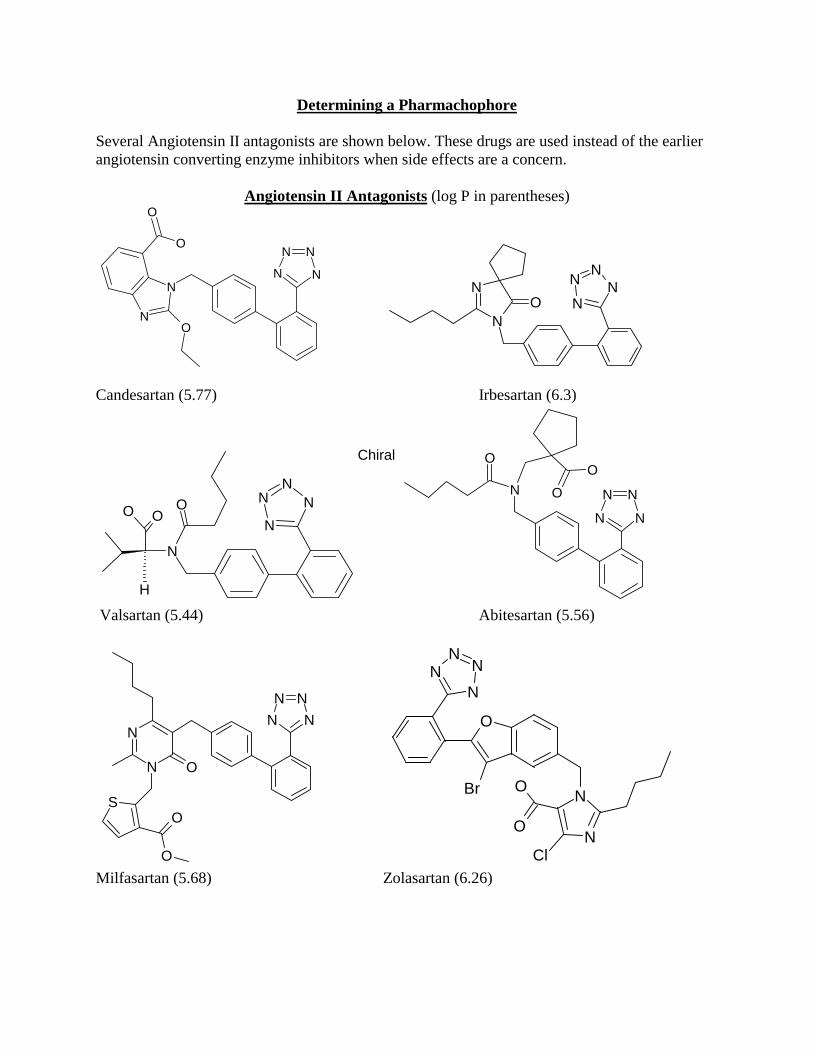
Determining a Pharmachophore Several Angiotensin II antagonists are shown below. These drugs are used instead of the earlier angiotensin converting enzyme inhibitors when side effects are a concern.

Angiotensin II Antagonists (log P in parentheses)

N

NO

O

O

NN

NN

N

NO

NN

NN

Candesartan (5.77) Irbesartan (6.3)

N

N

NN

N

OO O

H

Chiral

N

O

O

O

NN

NN

Valsartan (5.44) Abitesartan (5.56)

N N

N N

N

N O

S

O

O

O

Br

NN N

N

N

NCl

O

O

Milfasartan (5.68) Zolasartan (6.26)

A pharmachophore is a search query that will be used to search a database for other compounds that might have similar biological activity. One way to build a pharmachophore is to determine the simplest collection of functional groups that appear in common with a group of active compounds. There is no single correct answer for the pharmachophore. The best way to determine if a pharmachophore is useful is to use it in database searches. If the database search returns only compounds that are known to have the target biological activity then your pharmachophore is too specific. It is only finding compounds that you already know are active. If your pharmachophore produces thousands of database hits, it is too general. Thousands of hits would be impossible to sort through to determine which would be best for further testing. The best pharmachophore strikes a happy medium. The most useful pharmachophores return a large number of active compounds that are already in use. This ensures that you have chosen functional groups that are appropriate for the purpose. But the most useful pharmachophores also return compounds that have not been tested for biological activity for your target and also display some unusual structural features that you might not have thought of otherwise. In other words the best pharmachophore sparks your imagination about possible lead compounds without leading you down blind alleys. 1. Determine a pharmachophore that would fit all six of these compounds that would provide a minimum number of database search hits of other types of compounds. Be explicit about bond and atom types. Do your searches in the CMC3D database. An easy way to build your pharmachophore is to do a database search for the Class of angiotensin inhibitors to find one of the above compounds, for example

like “%angio%” will work. Then transfer this compound into Isis/Draw and erase the parts of the molecule that are not common to the other active compounds. Find a pharmachophore that recovers all six of the active compounds, but no more than about 30 total compounds. Report this pharmachophore. 2. Erase some additional part of your pharmachophore. Chose a part to erase that you feel would allow much additional flexibility, but at the same time won’t generate over 400 additional hits. Report this new pharmachophore and also give an example of a database hit that shows some new functionality not present in the original active compounds that you feel might be worth testing.