COMPUTED BEHAVIOR OF REINFORCED …shear walls behavior under these loads. Although there are many configurations and variations of shear wall systems in use, the analytical model

I PB 263 128) UILU-ENG-76-2024

CIVIL ENGINEERING STUDIESStructural Research Series No. 434

COMPUTED BEHAVIOR OF REINFORCED CONCRETECOUPLED SHEAR WALLS

byT. TAKAYANAGI

andw. C. SCHNOBRICH

A Report on a Research

Project Sponsored by

THE NATIONAL SCIENCE FOUNDATION

Research Grant ATA 7422962

UNIVERSITY OF ILLINOIS

AT URBANA-CHAMPAIGN

URBANA, IlliNOIS

DECEMBER 1976REPRODUCED BY

NATIONAL TECHNICAL~NFORMATION SERVICE

u. S. DEPARTMENT OF COMMERCESPRINGFIELD, VA. 22161

BIBLIOGRAPHIC DATA \1. Report No.SHEET UILU-ENG-76-2024 [2. 3. Recipient's Accession No.

4. Title and Subtitle

Computed Behavior of Reinforced Concrete-CoupledShear Walls

5. Report DateDecember 1976

6.

7. Author(s) T. Takayanagi and W. C. Schnobrich 8. Performini> Or&i'nization Rept.No. SR:.:> 4J4

9. Performing Organization Name and Address

University of Illinois at Urban~-Champaign

Urbana, Illinois 61801

12. Sponsoring Organization Name and Address

National Science FoundationWashington, D. C~ 20013

15. Supplementary Notes

16. Absrracts

10. Project/Task/Work Unit No.

11. Contract/Grant No.

ATA 7422962

13. Type of, Report & PeriodCovered

14.

The nonlinear response history and failure mechanism of coupledshear wall systems under dynamic loads and static loads are investigatedthrough an analytical model. The walls and coupling beams are replacedby flexural elements. The stiffness characteristics of each member aredetermined by inelastic properties.' The suitable hysteresis loops toeach constituent member are established to include the specificcharacteristics of coupled shear wall systems. The computed results arecompared with the available test results.

17. Key Words and Document Analysis. 170. Descriptors

Coupled shear walls, Nonlinear dynamic analysis, Earthquake engineering,Hysteresis loops, Equations of motion

17b~ Identifiers/Open-Ended Terms

17c. COSATI Field/Group

18. Availability Statement

Release Un14mited.II

FORM NTI5-35 (REV. 10-73) ENDORSED BY ANSI AND UNESCO.

19. Security Class (This.Report)

'TlNrl A

20. Security Class (ThisPage

UNCLASSIFIEDTHIS FORM MAY BE REPRODUCED

21. No. of Pages

19222. Price

USCOMM·DC 8265- P 74

ACKNOWLEDGMENT

The writers wish to express their sincere gratitude to Professor

Mete A. Sozen for his invaluable comments and help.

Deep appreciation is due Professor S. Otani of the University of

Toronto for his numerous suggestions and help.

Thanks are also due Dr. J. D. Aristizabal-Ochoa, Mr. J. M. Lybas,

and Mr. D. P. Abrams for providing the authors with information from

their test results.

The work was supported by a National Science Foundation Grant

No. ATA 7422962. The support is gratefully acknowledged.

III

Preceding pag@ blank

iv

TABLE OF CONTENTS

Page

CHAPTER

1. INTRODUCTION. . . . . . . . . . . . . . . . . . . . . . . . . . . . . . . . . . . . . . . . . . . . . . . . . . . . 1

1.1 Object and Scope.......................•................... 11. 2 Revi ew of Previous Research................................ 31.3 Notation 6

2. MECHANICAL MODEL " ""',' 0 •••••' •• ,.'••••':••• ',' ••• '12

2.1 Structural System.. , .. .' ;'." .•';;, 122.2 Mechanical Models of Connecting Beam and Wall. ," '.J, .' ..••.. 12

3. FORCE-DEFORMATION RELATIONSHIPS OF FRAME ELEMENTS 15

3.1 Material Properties '" 153.2 Moment-Curvature Relationship of a Section 173.3 Deformational Properties of Wall Subelements 193.4 Deformational Properties of the Rotational Springs

Positioned at the Beam Ends 24

4. ANALYTICAL PROCEDURE 35

4. 1 Introductory Remarks 354.2 Basic Assumptions 364.3 Stiffness Matrix of a Member 374.4 Structural Stiffness Matrix 474.5 Static Analysis 494.6 Dynamic Analysis 50

5. HYSTERESIS RULES ' 60

5.1 Hysteresis Rules byTakeda, et al. 605.2 Modifications of Takeda's Hysteresis Rules 60

6. ANALYTICAL RESULTS 63

6.1 Model Structures ~ 636.2 Static Analysis of Structure-l 646.3, Preliminary Remarks of Dynamic Analysis 716.4 Dynamic Analysis of Structure-l 736.5 Effects of Assumed Analytical Conditions

on Dynami c Response 816.6 Dynamic Analysis of Structure-2 86

v .

Page

7. SUMMARY AND CONCLUSIONS 91

7. 1 Obj ect and Scope........................................... 917.2 Conclusions 92

LIST OF REFERENCES ••••••••••••••••••••••••••••••••••••••••••• ; ••.••..•• 97

APPENDIX

A CALCULATIONS OF WALL STIFFNESS PROPERTIESIN THE COMPUTER PROGRAM 177

B COMPUTER PROGRAM FOR NONLINEAR RESPONSE ANALYSISOF COUPLED SHEAR ~JALLS •••••••••••••••••••••••••••••••••••••••••• 188

vi

LIST OF TABLES

Table Page

6.1 Assumed Material Properties 100

6.2 Stiffness Properties of Constituent Elements 10l

6.3 Summary of Assumed Analytical Conditions for Dynamic Runs 102

6.4 Mode Shapes and Frequencies of Structure-l 104

6.5 Maximum Responses of Structure-l in Comparisonwith Test Results 105

6.6 Effect of the Numerical Integration Schemeon the Maximum Responses of Structure-l 107

6.7 Effect of the Choice of Stiffness Matrixfor the Calculation of Damping Matrixon the Maximum Responses of Structure-l 108

6.8 Effect of the Arrangement of Wall Subelementson the Maximum Responses of Structure-l 109

6.9 Effects of the Pinching Action and Strength Decayof Beams on the Maximum Responses of Structure-l l10

6.10 Mode Shapes and Frequencies of Structure-2 112

6.11 Maximum Responses of Structure-2in Comparison with Test Results 113

vii

LIST OF FIGURES

Figure Page

2.1 Mechanical Model of Coupled Shear Wall System , 114

2.2 Connecting Beam Model .........................................• 115

2.3 Wall Member Model .......................................•...... 115

3.1 Idealized Stress-Strain Relationshipof Concrete 11 6

3.2 Idealized Stress-Strain Relationshipof Rei nforcement 116

3.3 Distributions of Stress and Strainover a Cross Section 117

3.4 Moment-Curvature Relationshipsof a Wall Member Secti on 118

3.5 Moment-Curvature Relationshipof a Connecting Beam Section 119

3.6 Idealized Moment-Curvature Relationshipsof a Wall Member Section 120

3.7 Idealized Moment-Curvature Relationshipof a Connecting Beam Section 121

3.8 Bond Slip Mechanism l22

3.9 Idealized Moment-Rotation Relationshipof a Rotational Spring 0 ••••••••••••••••• 123

4.1 Force and Displacement Components at Wall Member Ends 124

4.2 Cantilever Beam with Three Subelements ~ 124

4.3 Force and Displacement Components at Connecting Beam Ends 125

4.4 Moment Distribution of a Connecting Beam...............•....... 125

4.5 Deformed Configuration of a Connecting Beam 126

5.1 Takeda's Hysteresis Loops 127

5.2 Hysteresis Loops with Effect of Changing Axial Force 128

viii

Figure Page

5.3 Hysteresis Loops with Effects ofPinching Action and Strength Decay 129

6.1 Cross-Sectional Properties of Wall and Beam 130

6.2 Sequence of Cracking and Yielding of Structure-lunder Monotonically Increasing Load 131

6.3 Relationship of Base Axial Force and Top VerticalDisplacement of Walls of Structure-l underMonotonically Increasing Load 132

6.4 Base Moment-Top Displacement Relation of Structure-lunder Monotonically Increasing Load 133

6.5 Redistribution of Base Shear in Walls of Structure-lunder Monotonically Increasing Load 134

6.6 Ratio of Top Displacement due to Coupling Effectto Total Top Displacement of Structure-lunder Monoton ically Increas i ng Load 134

6.7 Base Moment Distribution Pattern of Structure-lunder Monotonically Increasing Load ~ 135

6.8 Moment Distribution Patterns in Members of Structure-lat the End of Monotonically Increasing Load 136

6.9 Base Moment-Top Displacement Relation of Structure-lunder Cyclic Loading 137

6.10 Waveforms of Base Accelerations 138

6.11 Initial Mode Shapes of Structure-l 139

6.12 Maximum Responses of Structure-l, Run-l,in Comparison with Test Results 140

6. 13 Response Waveforms of Structure-l, Run-l 142

6.14 Response Waveforms of Structure-l, Run-2 150


6.16 Response History of Base Moment-Top DisplacementRelationship of Structure-l, Run-l 152

6.17 Response Waveforms of Internal Forces of Structure-l, Run-l .... 153

ix

Figure Page

6.18 Hysteresis Loops of a Beam Rotational Springof Structure-l, Run-l 157

6.19 Hysteresis Loops of a Wall Subelement at Baseof Structure-l, Run-l 158

6.20 Sequence of Cracking and Yielding forDynami c Response of Structure-l, Run-l 159

6.21 Ratio of Coupling Base Moment to Total Base Momentat Peak Responses of ',tructure-l, Run-l 160

6.22 Ratio of Top Displacement due to Coupling Effectto Total Top Displacement at Peak Responsesof Structure-l, Run-l " 161

6.23 Coupling Effect of Walls on Displacement Distributionat the Maximum Response of Structure-l, Run-l 162






6.29 Response Waveforms of Structure-2, Run-10 168

6.30 Sequence of Cracking and Yielding forDynamic Response of S'ructure-2, Run-10 : 176

A.l Primary Curve for Hysteresis Loopsof a Wall Member Sect ion 184

A.2 Evaluation of .~~ for Hysteresis Loopsof a Wall Member Sect ion " 184

A.3 Axial Force-Axial Strain Relationshipof a Wall Member Section 185

A.4 Idealized Axial Force-Axial Strain Relationshipof a Wall Member Section 186

A.5 Relationship of Slope of Axial Force-Axial Strain Lineand Curvature for a Wall Member Section 187

B.l Flow Diagram of Computer Program for NonlinearResponse Analysis of Coupled Shear Walls 189

1

CHAPTER 1

INTRODUCTION

1.1 Object and Scope

The coupled shear wall is considered to be a very efficient structural

system to resist horizontal movements due to earthquake motions. It is

not possible to investigate thoroughly through model tests the influence

of the many possible variations in the various parameters that control the

response of coupled shear walls. The models are too expensive in terms

of both time and money. Furthermore, it is not always possible to record

when all the events of interest take place. On the other hand, most of

the papers dealing with the analysis of coupled shear walls are based on

elastic member properties. Those papers where inelastic member properties

are allowed are primarily for the case of monotonically increasing loads.

In view of the scarcity of data, it is necessary to investigate the

nonlinear response behavior of coupled shear walls due to strong

earthquake motions.

The study is intended to develop an analytical model which can trace

the response history and the failure mechanism of coupled shear walls

under dynamic and static loads and to see the characteristics of coupled

shear walls behavior under these loads.

Although there are many configurations and variations of shear wall

systems in use, the analytical model is discussed only with reference to

reinforced concrete coupled shear walls, two walls with connecting beams

under horizontal earthquake motions and static loadings.

2 .

To predict the actual behavior of coupled shear walls during strong

motion earthquakes, the dynamic structural properties in the highly

inelastic range are taken into consideration. Inelastic properties such

as cracking and crushing of the concrete, and yielding and bond slip of

reinforcing steel complicate the problem. Therefore, idealizations and

simplifications of the mechanical models for the constituent members are

considered necessary in the analytical procedure. The basic model used

in the study is composed of flexural line elements, both for the walls

and the connecting beams.

These constituent flexural elements incorporate their hysteretic

properties utilizing the test data available. The suitable hysteresis

loops to each constituent member are established by modifying Takeda's

hysteresis rules (1970)* to include the specific characteristics of

coupled shear walls.

The instantaneous nonlinear characteristics of the structure and

the failure process of each constituent member under strong earthquake

motions are estimated by numerically integrating the equation of motion

in a step-by-step procedure. Also the failure mechanism of the structure

under static loads is traced by constantly increasing lateral load at

small increments.

The computed results are compared with the available test results

by Aristizaba1-0choa (1976).

* References are arranged in alphabetical order in the List ofReferences. The number in parentheses refers to the year of publication.

3

1.2 Review of Previous Research

Analyses of coupled shear walls have been performed by many

investigators. No attempt will be made to cite all such reported

investigations. Only a few of the early and directly applicable studies

are referred to here.

A typical approach to the shear wall problem is the so-called

laminae method. In this method the discrete system of connecting beams

is replaced by a continuous connecting medium of equivalent stiffness.

Beck (1962) and Rosman (1964) analyzed coupled shear walls under lateral

loads based on this idealization. Coull (1968) extended this assumption

to take account of the shearing deformations of the walls. Later Tso and

Chan (1971) used this method to determine the fundamental frequency of

coupled shear wall structures. Such a determination is, of course,

essential in the application of the response spectrum technique. All

the papers mentioned above are based on linearly elastic properties of

the members.

Paulay (1970) used the laminae method to trace the failure mechanism

of coupled shear walls under monotonically increasing loads by introducing

plastic hinges at the ends of each lamina as well as at the base of wall

during the process of loading. Although the laminae method has the

advantage of being relatively simple to apply, this method cannot treat

the expansion of inelastic action over the length of the wall members.

The use of two dimensional plane stress elements with the finite

element method is another way of approaching the analysis of coupled

shear walls. Girijarallabhan (1969) used the element method in an attempt

to define more precise stress distributions of coupled shear walls.

4

Yuzugullu (1972) analyzed single-story shear walls and infilled frames

by using the finite element method, including in that analysis the

inelastic properties of reinforced concrete elements. Naturally this

approach is quite time-consuming for a multistory coupled shear wall

system. Such an analysis requires a very large number of elements.

Furthermore, difficulties arise in the wall element to beam element

connection. In order to avoid the use of plane stress elements for the

connecting beams, some means of establishing the rotational degree of

freedom at the wall connection must be introduced. One possibility is

a rigid arm from the wall center to the beam connection.

Instead ~f using the element method, inelastic beam models in which

each member is represented by a flexural line element were developed to

save the computing time and to simplify the mechanical model. Several

inelastic beam model techniques have been extensively used in the analysis

of the nonlinear response behavior of frame subjected to base excitations.

Clough, et a1. (1965) proposed the two component model to represent

a bilinear nondegrading hysteresis. The member consists of a combined

elastic member and an elasto-plastic member. Aoyama,et a1. (1968)

developed the four component model to represent the trilinear nondegrading

hysteresis loop. In this model the idealized beam has an elastic member

and three e1asto-plastic members in parallel. The four component model

and the two component model are based on the same concept. These models

are generally called mu1ticomponent models. The mu1ticomponent model has

some difficulties when applied to a degrading hysteresis system.

Giberson (1967) proposed the equivalent spring model which is

generally called the one component model. In this model rotational

5

springs, which represent only inelastic behavior of the beam, are

introduced at both ends of the beam. The rest of the beam, between the

ends, is considered to be elastic. This model has no coupling term in

the inelastic part of the flexibility matrix. In other words, the

inelastic rotation at one end is related only to the moment at the same

end and is independent of the moment at the other end. The inflection

point is assumed to be fixed at the same location during the response

behavior. This assumption is not realistic because the location of an

inflection point is expected to change during the real response behavior

of the beam. But this model is considered to be more versatile than the

mu1ticomponent model, since the rotational spring car. take care of any

kind of hysteresis loop.

Takizawa (1973) developed the prescribed flexibility distribution

model which is based on the assumption of a distribution pattern of cross

sectional flexural flexibility along the member axis. In his paper he

used a parabolic curve as the flexural flexibility distribution. The

inflection point is not necessarily fixed in this model.

Otani (1972) presented the combined two cantil ever beam model. The

beam consists of two cantilever beams whose free ends are placed at the

inflection point. The beam is not allowed to be subjected to any change

of the moment distribution which produces a serious sudden movement of

the inflection point. But this model has very natural correspondence

between the actual phenomena and the available hysteresis data based on

the test result.

Hsu (1974) investigated the inelastic dynamic response of the single

shear wall experimentally and analytically. In the analytical part of

6

his study, he assumed a divided element beam model in which the beam is

divided into several elements and each element has a uniform flexural

rigidity changeable based on the hysteresis loop. In this model it is

easy to handle a local concentration of inelastic action of the member

by arranging elements finely at the location of interest.

1.3 Notation

The symbols used in this text are defined where they first appear.

A convenient summary of the symbols used is given below.

As = area of the tensile reinforcement

AI = area of the compressive reinforcementsb = width of the cross section

c = depth of the neutral axis

c l = distance from the neutral axis to the point of

the maximum tensile stress of the concrete

cl ' c2 = coefficients for the damping matrix

[C] = damping matrix

[Cc] = instantaneous damping matrix which is evaluated

at the end of previous step

d = distance from the extreme compressive fiber to

the center of tensile reinforcement

d' = distance from the extreme compressive fiber

to the center of compressive reinforcement

D = total depth of a section or diameter of a reinforcing bar

Dc = cracking displacement of the unit length cantilever beam

D = yielding displacement of the unit length cantilever beamy

7

Du = ultimate displacement of the unit length cantilever beam

D(M) = free end displacement of a cantilever beam

Es =modulus of elasticity of the steel

Eh = modulus to define stiffness in strain hardening range

of the steel

Ey = inelastic modulus of the reinforcement after yielding

EA. = inelastic axial rigidity of a section.1

EI = initial flexural rigidity

EI e = elastic flexural rigidity of a section

Eli = inelastic flexural rigidity of a section

Ely = ratio of flexural rigidity after yieldin~ to that

before yielding

f = stress of the concretec

f' = compressive strength of the concretec

f t = tensile strength of the concrete

f s = stress of the steel or stress of the tensile reinforcement

f' = stress of the compressive reinforcements

fy = yield stress of the steel

fu = ultimate stress of the steel

f(M) = flexibility resulting from the bomd slippage

of tensile reinforcement of a beam

[fAB] = flexibility matrix of a cantilever beam

GAe = elastic shear rigidity of a section

GA. = inelastic shear rigidity of a section1

[K] = structural stiffness matrix

[K .. ] = submatrices used in Eq. (4.16) 0,j = 1 or 2)1J

[KAB] = stiffness matrix of a cantilever beam

8,

[Kc] = instantaneous structural stiffness matrix

which is evaluated at the end of current step

[Ke] = elastic structural stiffness matrix

[K.] = inelastic structural stiffness matrix,[Kw] = stiffness matrix of a wall member

£. = length of the subselement i,L = length of a beam or development length of the bond stress

~L = elongation of the reinforcment

m = bending moment of a section

~m = increment of bending moment

m. = lumped mass at the story i,M= bending moment

M = cracking momentcMy = yielding moment

Mu = moment at concrete strain equal to 0.004

M(¢,n) = bending moment function

~M = increment of moment

~MA' ~MB = incremental moments at the ends of a member

~Mc' Mb = incrementa 1 end moments of the flexible element

of a connecting beam

{~M} = incremental joint moment vector

[M] = diagonal mass matrix

n = axial force of a section

~n = increment of axial force

N - axial load acting on a section

N(¢, s) = axial force function

9

~A' ~B = incremental shear forces at the ends of a connecting beam

or incremental axial forces at the ends of a wall member

{~} = incremental joint vertical force vector

6PA, ~PB = incremental shear forces at the ends of a wall member

{~P} = incremental story lateral force vector

R = rotation due to the reinforcement slip at the end of

a connecting beam

Rc = rotation at which the cracking moment is developed

R = rotation at which the yielding moment is developedy

R = rotation at which the ultimate moment is developedu

SD(M) = instantaneous stiffness of the unit length cantilever

beam based on the flexural rigidity

ST(M) = instantaneous stiffness of the unit length cantilever

beam based on the flexural and shear rigidities

~t = time interval

[TAB] = transformation matrix of a cantilever beam

u = average bond stress

~UA' ~UB = incremental lateral displacement at the ends of a wall member

{~U} = incremental story lateral displacement vector or incremental

story displacement vector relative to the base

{~U} = incremental story velocity vector relative to the base~.

{6U} = incremental story acceleration vector relative to the base

{U} = relative story velocity vector at the end of previous step

{U} = relative story acceleration vector at the end of previous step

6V = increment of the free end displacement of a cantilever beam

10'

fc,V f = increment of the free end displacement of a cantilever beam

only due to the flexural rigidity

fc,VA, fc,V B = incremental vertical displacement of a member

{fc,V} = incremental joint vertical displacement vector

{fc,X} = incremental base acceleration vector

Z = constant which defines the descending slope of the

stress-strain curve of the concrete

8 = constant of the Newmark ~ method

8i = damping factor of the i th mode

Y = ( / )1/2wi we

£ = axial strain of a section

fc,£ = increment of axial strain

£c = strain of the concrete or concrete strain

at the extreme compressive fiber

£0 = strain at which f~ is attained

£t = strain at which f t is attached

£s = strain at the steel or strain in the tensile reinforcement

£~ = strain in the compressive reinforcement

£y strain at which fy is attained

£h = strain at which strain hardening of the steel commences

£u = strain at which fu is attached

n = distance from the neutral axis of a section

fc,8 = increment of rotation

M A, M 1 = incremental rotations at the ends of a memberBM

A, fc,8 B = incremental rotations at the rigid link ends

of a simply supported beam

11

~ec' ~eD = incremental and rotations of the combined spring-flexible

element of a connecting beam

{~e} = incremental joint rotation vector

A = ratio of the length of a rigid link to that of a flexible

element for a connecting beam

<P = curvature

<Pc = curvature at cracking

<Py = curvature at yielding

<P u = curvature at concrete strain equal to 0.004

~<p = increment of curvature

{~} = first mode shape vector

wj = circular frequency of the jth mode

we = first mode circular frequency in the elastic stage

wi = first mode circular frequency in the inelastic stage

12

CHAPTER 2

MECHANICAL MODEL

2.1 Structural System

The lateral resistance of coupled shear walls results primarily from

three sources of structural actions: the flexural rigidity of the walls,

the flexural rigidity of the connecting beams and the moment effect of the

couple growing out of the axial rigidity of the two walls.

The mechanical model chosen to represent the coupled shear walls is

shown in Fig. 2.1. The walls and the connecting beams are replaced by

massless line members at their centroidal axes. The wall members have

flexural, axial and shear rigidities as their resistances. The connecting

beam members have flexural and shear rigidities. The axial rigidity of

the connecting beam is assumed to be infinite since the horizontal

displacements of both walls are practically identical.

Three displacement components are considered at each wall-beam joint:

horizontal displacement, vertical displacement and rotation. The right

hand screw rule is adopted to describe the positive directions of these

displacement components as shown in Fig. 2.1.

The internal subelements or degrees of freedom are condensed out of

the stiffness matrix before the system equations are written so that

only horizontal story movements appear in the final equations. The mass

of each story is assumed to be concentrated at each floor level. In the

analysis the wall is considered to be fixed at the base.

2.2 Mechanical Models of Connecting Beam and Wall

A mechanical model of the connecting beams used in the study is the

one which Otani (1972) developed based on inelastic actions of a cantilever

13

beam. This model is quite suitable for the connecting beams of a

coupled shear wall system~ since the contraflexure point is practically

fixed at the center of the beam span during its response.

The connecting beams are taken as individual beams connected to the

walls through a rigid link and a rotational spring as shown in Fig. 2.2.

The rotational spring takes care of any beam end rotation which is

produced by the steel bar elongation and concrete compression in the

joint core area as well as the inelastic flexural and shear actions over

the beam length. Such inelastic flexural action is expected to be

localized near the beam ends because of the antisymmetric moment

distribution over the beam length. The action within the joint core

could have been treated by the effective length concept in which the

clear span length of beam is arbitrarily expanded into the joint core to

allow for flexural and slip action in the joint core. But it was judged

much simpler to consider the joint core as a rigid link and to let the

rotational spring take care of the inelastic and other actions of the

joint core area. The beam itself is considered to be a flexural member

with uniform elastic rigidity along its length.

The wall is also considered to act initially as a beam with a

linear variation of strain over the cross section. To use two-dimensional

plane stress elements for the walls was judged less desirable~ since such

an approach would have been much more expensive computationally without

any compensating increase in accuracy. It is in fact probable that while

accounting for cracking and nonlinear action of the plane stress elements

with current concepts and methods the system would not reproduce

experimental results as well as line elements can.

14

The wall members are exposed to a more general moment distribution

than are the connecting beams. In addition, the location of the

contraflexure point might shift significantly from a change in the moment

distribution and the change of axial force during the response might cause

a change of moment capacity in the wall members. Therefore the inelastic

flexural behavior in the wall can be expected to expand along the length

of the member rather than be localized. In order to allow the inelastic

action to cover a partial length of a wall member, the member is further

divided into several subelements as shown in Fig. 2.3. The stress

resultants at the centroid of the subelements are used as the control

factors for the determination of the nonlinear properties of the

subelements. The degree of subdivision decreases with story height

since the major inelastic action is expected at the base.

15

CHAPTER 3

FORCE-DEFORMATION RELATIONSHIPS OF FRAME ELEMENTS

3.1 Material Properties

Inelastic force-deformation relationships for the wall subelements

and corresponding relationships for the rotational springs placed at the

connecting beam ends are based on idealized stress-strain relationships

for concrete and steel. These inelastic force-deformation relationships

are used as the primary curves for the hysteresis loop.

(a) Stress-Strain Relationship for Concrete

A parabola combined with a straight line in the form used by Otani

(1972) is also adopted here for the stress-strain relationship of concrete.

Accordingly,

and

where

f = a I:: < Stc c -

E: E: 2f = f' [2~ - (~) ] I::t < I:: < I::

C C 1::0

1::0

- C - 0

f = fl[l - Z(E - EO)] E < SC C C o - c

1

E = E [1 - (1 - f / f I )'2]tot c

f = stress of the concretec

f" = compressive uniaxial strength of the concretec

f t = tensile strength of the concrete

Et = strain of the concrete

(3. 1 )

f

)

(3.2)

(3.3)

16'

S = strain at which fl is attainedo c

St = strain at which f t is attained

Z = constant which defines the descending slope

of the stress-strain curve. The value of 100

was used in this analysis.

Justification for the use of these relations can be found in Otani's

thesis. A typical example of the proposed curve is shown in Fig. 3.1.

(b) Stress-Strain Relationship of Steel

A piecewise linear stress-strain relationship is assumed for the

reinforcing steel. Accordingly,

f s = Es Ss S < SS -y

fs = fy E < E < EhY -- s-

fs = f + Eh(Es - Eh) sh < S < SY -- s - u

fs - f u E < SU - S

where

f s = stress of the steel

fy = yield stress of the steel

f u = ultimate stress of the steel

Ss = strain of the steel

Sy = strain at which fy is attained

Eh = strain at which strain hardening commences

EU = strain at which f is attainedu

Es = modulus of elasticity of the steel

Eh = modulus to define stiffness in strain hardening range

(3.4)

17

The numerical value of Es is assumed to be 29,000 kip/in. 2 in the

analysis. The representative stress-strain curve of the steel is shown

in Fig. 3.2. The stress-strain relations represented by Eqs. (3.4) are

assumed to be symmetric about the origin.

3.2 Moment-Curvature Relationship of a Section

The primary moment-curvature curve for a monotonically increasing

moment can be derived based on the geometry of the section, the existing

axial load, the deformational properties of concrete and steel mentioned

in Section 3.1, and the assumption that a linear variation of strain

exists across the cross ection. This linear variation is maintained

throughout the entire loading.

The relationship of curvature of a section to strain can be expressed

by utilizing the assumption of linear strain distribution. This is shown

in Fig. 3.3. The relation takes the following forms.

cjJ = s/c

= s~/(c d I) (3.5)

= s/(d c)

where

cjJ = curvature

Sc concrete strain at the extreme compressive fiber

I = strain in the compressive reinforcementSs

Ss = strain in the tensile reinforcement

d l = distance from the extreme compressive fiber

to the center of compressive reinforcement

18

d = distance from the extreme compressive fiber

to the center of tensile reinforcement

c = depth of the neutral axis

The equilibrium equation of the resultant forces can be expressed

as follows:

fc f

c b dx + Al f' - A f = Ns s s s-c'

where

fl = stress of the compressive reinforcementsf s = stress of the tensile reinforcement

b = width of the cross section

AI = area of the compressive reinforcements

As = area of the tensile reinforcement

N = axial load acting on the section

c' = distance from the neutral axis to the point

of the maximum tensile stress of the concrete

The bending moment Mat the depth x can be calculated by the

following equation.

M== Jc fc bndn + (x - c) Jc fc b dx + A~f ~ (x - d')-c' -c'

where

o = total depth of the section

n = distance from the neutral axis

(3.6)

(3.7)

The stresses fc~ f~ and f s can be calculated by Eqs. (3.1) and (3.4) for

19

given strains EC

' E~ and ES

' respectively.

It is difficult to solve Eqs. (3.5) and (3.6) directly for the unknowns

sc and c, because the solution may not be available in a closed form.

Therefore a recommended procedure is that Eqs. (3.5) and (3.6) are solved for

c with given EC

and N by the iteration method. The moment Mand' curvature

¢ can be derived by Eqs. (3.5\ and (3,n with a calculated c and a given sc'

The bending moment Mis evaluated along the plastic centroid of the section.

The moment-curvature curve can be drawn by the series of calculated Mand

¢ for different values of EC

'

Flexural cracking of a reinforced concrete section subjected to both

flexural and axial load is assumed to occur when the stress at the extreme

tensile fiber of the section exceeds the tensile strength of concrete.

Flexural yielding is considered to occur when the tensile reinforcement

yields in tension. If the tensile reinforcement is arranged in many layers,

the stiffness change occurs gradually starting with the initiation of

yielding of the furthest layer of reinforcement and proceeding until

yielding occurs in the closest layer to the neutral axis of the section.

Because of the requirement of the hysteresis rules used in this analysis,

a single value of the yield moment is to be given. Therefore the yield

moment is defined as the moment corresponding to the development of the

yield strain at the centroid of the reinforcing working in tension.

Typical examples of moment-curvature curves for a wall section and

a beam section are shown in Fig. 3.4 and Fig. 3.5, respectively.

3.3 Deformational Properties of Wall Subelements

The inelastic moment-curvature relationships of the wall subelements

are used as the primary curves in establishing the hysteresis loops.

20,

The stress resultants computed at the centroid of each subelement are

used in the determination of the instantaneous stiffness of the subelement

so that each subelement can be subjected to a different stage of

non1i nea rity.

Each subelement has three types of rigidities: flexural, axial and

shear. The instantaneous flexural rigidity of each subelement is defined

as the slope of the idealized moment-curvature curve at the point which is

located by the history of ineOlastic action in the subelement.

To simplify the problem this idealized moment-curvature relationship

is determined by trilinearizing the original moment-curvature curve. The

slopes in the three stages of this idealized moment-curvature relatinship

are defined as foll ows:~1

ep = M/(/)c

M - M<P = Mj(......l.-~) + <P

<Py - <Pc c

M - M<P = Mj(_U_-L) + <P

<P u <Pyy

where

M< M- c

M < M< Mc - - y

M < MY - .

(3.8)

M= bending moment

MC

= cracking moment

My = yielding moment

Mu = moment at concrete strain equal to 0.004

<P = curvature

<Pc = curvature at cracking

<P = curvature at yieldingy

<p = curvature at concrete strain equal to 0.004u

21

A series of idealized moment-curvature relationships for different

values of constant axial force are shown in Fig. 3.6. Actually the axial

force on a section is not constant and is subject to change in the process

of loading. The moment-curvature curve of a section under a changing axial

load is traced by appropriate shifts or movements between the series of

moment-curvature curves for constant axial loads as shown by the dashed line

in Fig. 3.6. It is assumed that the axial force is small enough that the

interaction curve is in the linear range, about the zero axial force axis.

Cases where the axial compressive forces are near or above the balance

point are not considered.

The axial rigidity is affected by cracking depth and any inelastic

conditions of the steel and concrete. With an aim to simplifying the

problem, it is assumed that the axial rigidity is only related to the

curvature and axial strain of the section. Therefore the bending moment

and axial force of a section are correlated to each other. A procedure

to calculate the instantaneous inelastic flexural and axial rigidities of

a section, in which the effect of axial force on the moment-curvature

curve and the effect of curvature on the axial force-axial strain curve

are taken into account, is developed in this study.

The moment is assumed to be a function of curvature and axial force,

while the axial force is a function of curvature and axial strain.

where

m= M(~,n)

n = N(~,E)

m = bending moment of a section

n = axial force of a section

M= bending moment function

} (3.9)

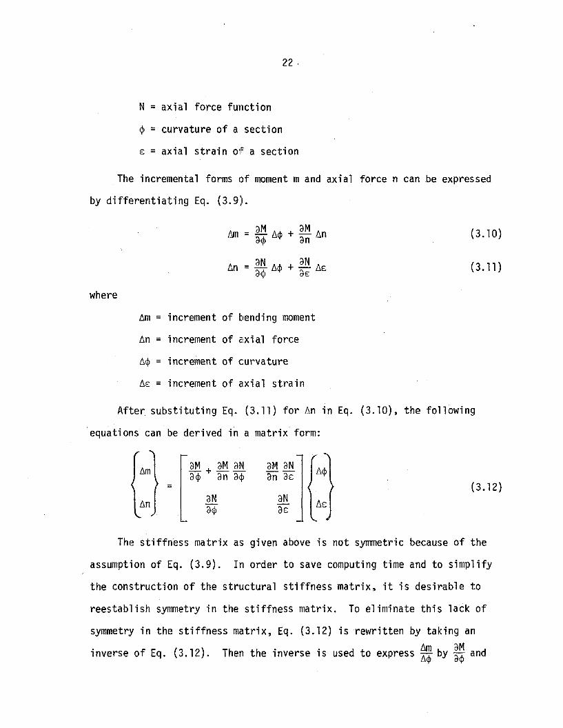
22 .

N = axial force function

¢ = curvature of a section

E = axial strain of a section

The incremental forms of moment mand axial force n can be expressed

by differentiating Eq. (3.9).

lim = aM li¢ + aM lina¢ an

lin =~ li¢ + aN liEa¢ aE

where

lim = increment of bending moment

lin = increment of axial force

li¢ = increment of curvature

liE = increment of axial strain

(3.10)

(3.11)

After substituting Eq. (3.11) for lin in Eq. (3.10), the following

equations can be derived in a matrix form:

lim aM + aM aN.. aM aNa¢ an a¢ ana£"

= (3.12)lin aN aN

a¢ aE

The stiffness matrix as given above is not symmetric because of the

assumption of Eq. (3.9). In order to save computing time and to simplify

the construction of the structural stiffness matrix, it is desirable to

reestablish symmetry in the stiffness matrix. To eliminate this lack of

symmetry in the stiffness matrix, Eq. (3.12) is rewritten by taking anlim aMinverse of Eq. (3.12). Then the inverse is used to express li¢ by a¢ and

23

Lm aNa modification factor and ~E by aE and a modification factor as follows:

~n

=

r (aMa¢ 1

a

1 )aN aM f~m .aM(a¢ / a¢h~n - an)

(3.13)

It is assumed that the ratio of the increment of axial force over that

of moment ~~ does not change markedly during the loading process. Therefore

the previous step value of ~~ is used for the matrix terms in Eq. (3.13) to

avoid the necessity of an iteration process.

The value of ~~ can be derived from the idealized moment-curvature

hysteresis loop for the corresponding axial force acting on the section.

The value of ~~ can be calculated by referring to the idealized axial

force-axial strain curve for a given curvature. The detailed procedure foro aM aN aN aM °evaluatlng 3¢' as' a¢ and an ln the computer program is schematically

explained in Appendix A.

The current effective flexural rigidity E1. and current effective1

axial rigidity EAi are considered as

= aM ( 1 \Eli a¢ 1 _ aM ~)

an am

EA=~( 1 )i aE 1 _ (~/ aM)(~ _ aM)a¢ d¢ ~n an

(3.14)

(3.15)

° hOh aM ddN °d d d OOdOtO Th tln w lC d¢ an dE are conSl ere as pseu o-rlgl 1 les. e curren

effective flexural rigidity represents the slope of the moment-curvature

relationship, including the effect of a changing axial force. The pseudo-

24

flexural rigidity is the slope of the moment~curvature relationship with

a constant axial force acting.

The evaluation of the shear deformation of a member in an inelastic

range is complicated with the existence of both axial force and moment.

In addition, the shear deformation is considered to be of a secondary

effect to the entire deformation while the flexural deformation is dominant.

Therefore it is considered acceptable to employ the assumption that the

inelastic values of shear rigidity reduce in direct proportion to those of

flexural rigidity. The equation stating this assumption can be expressed

in the form,

where

EI.GA. =·EI' GA, e e

GA. = inelastic shear rigidity,GAe = elastic shear rigidity

EI. = inelastic flexural rigidity,EI = elastic flexural rigiditye

(3.16)

These rigidities of the wall subelements are used for the development of

the member stiffness in the analysis.

3.4 Deformational Properties of the Rotational Springs Positionedat the Beam Ends

Rotational springs are placed at the ends of each connecting beam

to take care of the rotation due to inelastic flexural action in the beam,

bond slippage at the ends of the beam, and shear deformation within the

span of the beam.

25

Inelastic flexural action in the connecting beam is assumed to be

localized at the ends of the beam since the beam is exposed to antisymmetric

moment distribution along its length. There is a natural correspondence

between the deformational properties of the rotational springs and the

fixed and moment-free end displacement relationship of a cantilever beam,

since end rotations of a simply supported member subjected to an anti

symmetric moment distribution can be related to the deformations of two

cantilevers as discussed by Otani (1972). Therefore the deformational

properties of the rotational springs in the inelastic region can be derived

by calculating the moment-displacement curve of a cantilever whose span is

half the length of the connecting beam span. This assumes the point of

contraflexure is fixed at midspan of the connecting beam. To make the

procedure applicable to beams with arbitrary length, a cantilever with

unit length is considered in the analysis.

(a) Idealized Moment Curvature Relationship

An idealized moment-curvature relationship for the connecting beams

is developed to compute the free end displacement of a cantilever beam.

The moment-curvature relationship is idealized by three straight lines

as shown in Fig. 3.7.

where

M¢ = IT M< M- - c

M < M< Mc - - y

M < My-

(3.17)

26 .

E1 = initial fl exuralri gi di ty

EI = ratio of flexural rigidity after yielding to thaty

before yieldin'9

For a given moment, the curvature is calculated by Eq. (3.17).

(b) Rotation due to Inelastic Flexural Action Based on IdealizedMoment-Displacement Relationship of a Cantilever Beam

As the bending moment is distributed linearly over the length of the

cantilever replacement of the connecting beam with zero moment at the free

end and the maximum moment at the fixed end, the curvature distribution

can be defined for a given fixed end moment by Eq. (3.17). Displacement

at the free end of the cantilever beam is then calculated from the curvature

distribution by computing the first moment of the curvature diagram about

the free end.

The free end displacement D(M) can be expressed as the function of

the fixed end moment Mby equations of the form

L2 MD(M) = 3" IT

L2 3M 2D(M) = -- [(l-a ) ¢ -- + a ¢ J3 y My c

2D(M) = L6 [(2+8)(1-S){8 + Ei (1-8)}

y

+ 8(1+B) - 2a3J i + L32

a2¢c

where

L = length of the cantilever beam

:; Mca = M

M8 = i

M< M- c

M < M < Mc "- - y

M < My-

(3.18)

27

With the moment-displacement relationship of a cantilever beam with

unit length available, the relationship for a cantilever beam with any

length can be derived by simply multiplying the relationship for a unit

length cantilever by the square of the length for the desired span since

the free end displacement is always proportional to the square of the

length of the cantilever.

The idealized moment-displacement curve of a unit length cantilever

is calculated by trilinearizing the original curve, that is, connecting

the origin, cracking, yielding and ultimate points successively by straight

lines. The ultimate moment is defined as the point when the extreme

compressive fiber strain reaches 0.004.

The cracking, yielding and ultimate displacements of the unit length

cantilever can thus be expressed as:

(3.19)- s ).}u

where

o = cracking displacement of the unit length cantileverc0y = yielding displacement of the unit length cantilever

o = ultimate displacement of the unit length cantileveru

_ Mcay - r"y

Mcau = M

u

28 '

M8 ::;--Xu M

u

Slopes in the three sta~les of the idealized moment-displacement

relationship are defined as follows:

where

SD(M)_ Mc-~

M - MSD(M) ::; Y c

o - Dy c

Mu - MSD(M) ::; Y

Du - 0y

M< M- c

M < M< Mc - - y

M < My-

(3.20)

SD(M) ::; instantaneous stiffness of the cantilever beam

of unit 1en~Jth

The incremental rotation of the rotational spring due to inelastic

flexural action can be expressed approximately by the instantaneous

stiffness SD(M) since inelastic flexural action is assumed to be localized

at the beam end. Accordingly,

L1.J.8 ::; 2SDU~) ~M

where

~8 ::; increment of rotation

~M ::; increment of moment

L ::; length of beam

(3.21)

Equation (3.21) is used as a part of the instantaneous moment-rotation

relationship of the rotational springs in the analysis.

29

(c) Rotation due to Inelastic Shear Deformation

In addition to the flexural deformation of the connecting beams,

rotation due to shear deformation of the beams is also taken into

account in this study. The ratio of the shear displacement to the total

displacement of a cantilever beam is considered as a modifying factor

to be applied to the instantaneous stiffness SD(M) which originally

included only the inelastic flexural deformation.

Based on the reasoning discussed in Sec. 3.3, it is assumed that

the inelastic shear rigidity reduces in direct proportion to the

inelastic flexural rigidity.

The incremental free end displacement due to both shear and flexural

deformations in a cantilever beam that result from a given incremental

triangular moment distribution can be expressed as follows:

L L3 ~Mf.,V = (GA. + 3EI) T

1 1

where

f.,V = increment of the free end displacement

L = length of the cantilever beam

f.,M = increment of the fixed end moment

(3.22)

The ratio of the incremental displacement based solely on flexural

rigidity to that based on both flexural and shear rigidities is considered

to remain constant during any stage of inelastic action. The inelastic

flexural rigidity Eli is assumed to be uniformly distributed along the

length of the cantilever beam, although the actual inelastic flexural

rigidity is likely to develop near the fixed end of the cantilever beam.

Therefore the instantaneous stiffness of the cantilever can be modified

30

for the case which includes shear deformations as well as flexural

deformations by simply multiplying SD(M) by the ratio of the flexural

displacement to the sum of flexural and shear displacements. The

displacement ratio is

t1V f _ 1 1=t1V - 3EI i 3ET e--+ 1 2 + 1

GA. L2 GAe L,since

where

EI = elastic flexural rigiditye

GA = elastic shear rigiditye

Thus the stiffness can be expressed as:

(3.23)

ST(M)

where

(3.24)

t1V = incremental displacement due only to flexural rigidityfSD(M) = instantaneous stiffness based on flexural rigidity

ST(M) = instantaneous stiffness based on flexural and shear rigidity

For the case when the rotation due to shear deformation is considered

in the analyses, the instantaneous stiffness ST(M) is used instead of

SD(M) in Eq. (3.21).

(d) Rotation due to Bond Slippage at the Ends of the Beams

Rotation due to the slip of the tensile reinforcement of the beam

along its embedded length is considered as an additional flexibility factor

31

for the rotational spring at the ends of a beam.

Bond stress is assumed to be constant along the embedded length of

the reinforcement. Therefore the tensile force of the reinforcement is

transmitted into the concrete in such a way that the steel stress

decreases linearly with distance in from the wallface.

It is assumed that the reinforcement embedment length is sufficient

to provide the maximum tensile stress that occurs in the response

calculations. The development length L can be computed from the

equilibrium of forces as follows:

(3.25)

where

As = cross sectional area of the tensile reinforcement

f s = stress of the reinforcement at the face of wall

o = diameter of a reinforcing bar

u = average bond stress

The strain hardening portion for the reinforcement is idealized by a

line which connects the yield point and the point at the maximum strength.

The elongation of the reinforcement over the development length is

calculated by integrating the strain over the length.

If the stress of the reinforcement exceeds the yield stress fy ' the

development length is divided into two parts, as shown in Fig. 3.8. This

is done to accommodate the change in the reinforcement's axial rigidity.

Therefore the integration of the strain must be performed separately over

the two parts of the development length, that is, from the point of zero

stress to that of the yield stress and from the point of the yield stress

32·

to that of the maximum stress.

The elongations of the reinforcement are calculated as:

where

LfS

.6.L = 2Es

L fy2 L + (1 fv)(fv f s - fy ) L.6. = 2f E - fL E + 2E-

s s s s y

.6.L = elongation of the reinforcement

E = Young's modulus of the reinforcements

E = inelastic modulus of the reinforcementy

f < fs - y

f < fY - s

(3.26)

(3.27)

after yielding is developed

fy = yielding stress of the reinforcement

The elongation can be rewritten by substituting Eq. (3.25) for L in

Eqs. (3.26) and (3.27), and by replacing As by i 02 The result is

f < fs - y

f < f. y - s

(3.28)

(3.29)

It is assumed that the compressive reinforcement does not slip and

the concrete in the joint is rigid. Therefore the rotation due to bond

slippage can be expressed as follows:

where

.6.LR = d - d'

R = rotation due to the slip at the ends of a beam

d = depth of the tensile reinforcement

d' = depth of the compressive reinforcement

(3.30)

33

In order to have a rotation-moment relationship rather than the

rotation-stress one, the relation between bending moment and stress is

assumed in the form

where

M= bending moment at the end of a beam

M = yielding moment at the end of a beamy

By using Eq. (3.28) through Eq. (3.31), the rotation-moment

relationship c~n be expressed as follows:

M< M- Y

+ _1_ (lL _ 1)2] 12E

yMy -:"d-----:"d..,-'

M < My-

(3.31)

(3.32)

(3.33)

The idealized form of the rotation-moment relationship is obtained

by trilinearizing the original curve, that is, connecting the origin,

cracking, yielding and ultimate moments successively for simplification

of the problem.

These break points for the trilinearization' can be expressed as

follows:

1 Mu 2 1+ 2E (M - 1) ] d - d I

Y Y

(3.34)

34 .

where

R = rotation at whiich the cracking moment is developedc

R = rotation at which the yielding moment is developedy

R = rotation at whiich the ultimate moment is developedu

The flexibilities in thE~ three stages of the idealized rotation-

moment relationship are defined as follows:

f(M)Rc M< M=M - ccR - R

f(M) = Y (~ Me ~ M~ My (3.35)M - My c:

f(M) =Ru - Ry_

M < MMu - My y-

where

f(M) = flexibility resulting from the bond slippage of

tensile reinforcement of a beam)

The incremental rotation of the rotational spring due to bond slippage

can be expressed by the flexibility f(M), as follows:

!J.e = f(M) !J.M (3.36)

Equation (3.36) is used as a part of the instantaneous moment-rotation

relationship of a rotational spring in the analysis.

The calculated moment-rotation curve of a rotational spring including

flexural and shear actions over the beam length and bond slip in the joint

core is compared with the test result by Abrams (1976) in Fig. 3.9.

35

CHAPTER 4

ANALYTICAL PROCEDURE

4.1 Introductory Remarks

This chapter describes a method of analysis for reinforced concrete

coupled shear wall structures subjected to static loads and dynamic base

excitations. The analytical procedure is developed to study the behavior

of a structural system as well as that of its constituent members even

when that system is loaded into a highly inelastic range.

The constituent member stiffnesses are evaluated based upon the

force-deformation relationships of the rotational springs of the beam and

the subelements of the wall as described in Chapter 3. The instantaneous

structural stiffness matrix is developed by assembling the constituent

member stiffnesses and then condensing out all degrees-of-freedom except

those for the horizontal story movements. Only those degrees-of-freedom

remain in the final equations.

The mass of the structure is considered to be concentrated at each

floor level so that the lumped mass concept can be used in the analysis.

The damping matrix is evaluated as the sum of a part proportional to the

mass matrix and a part proportional to the structural stiffness matrix.

The inelastic behavior of the structure under static loads is

evaluated by applying a known set of lateral loads to the structure.

These loads are applied in very small increments. The inelastic dynamic

response and failure process of the structure under dynamic base motions

are calculated by numerically integrating the equations of motion with a

step-by-step procedure, Tung and Newmark (1954).

36

The effect of load history in each constituent element is taken care

of by using a set of hysteresis rules. These rules are an adaptation of

those presented by Takeda, et a1. (1970). A computer program has been

developed to apply the analytical procedure to the analysis of coupled

wall structures. The program is briefly explained in Appendix B.

4.2 Basic Assumptions

In this section the basic assumptions used in the analysis in order

to simplify the solution of the problem are presented.

(1) The analysis is limited to plane frame problems. Out-of-p1ane

action is ignored in the analysis. Three independent displacements are

considered at each joint: two mutually perpendicular translations in a

plane and one rotation about an axis normal to the plane.

(2) The right-hand screw rule is adopted to describe the global

coordinate system as well as the member coordinate system.

(3) Every member in the structure is considered as a massless line

member represented by its cE!ntroida1 axis.

(4) Geometric nonlinearity is ignored in the analysis. Small

deformations are assumed in the analysis so that the calculation of

inelastic response of the structure can be based on the initial

configuration.

(5) The idealized frame is assumed to be fixed at the base of the

structure which rests on an infinitely rigid foundation.

(6) The mass of the structure is assumed to be lumped at each

story level.

37

(7) The inelastic deformation of each constituent member is

assumed to follow the Takeda's hysteresis rules.

(8) The instantaneous nonlinear characteristics of the structure

are assumed to be constant within a time interval or a load step interval.

(9) Shear deformation in a joint core is ignored in the analysis.

(10) Only horizontal base motion is considered as the external

dynamic force applied to the structure.

(11) The axial elongation of the connecting beams is ignored so that

the two walls move horizontally at the same rate.

(12) p-~ effect is ignored in the analysis.

4.3 Stiffness Matrix of a Member

This section describes the ways to develop the stiffness matrix of

each constituent member of the structure such as the connecting beams and

walls based upon the force-deformation relationships of frame elements

mentioned in Chapter 3.

(a) Wall Member

A wall member has axial force, shear force and bending moment as its

force components. Vertical displacement, horizontal displacement and

rotation are the displacement components at the ends of each wall member.

These member forces and displacements, together with their positive

directions, are shown in Fig. 4.1.

Each wall member is considered to consist of several subelements

so that each subelement can be subjected to a different stage of inelastic

action. The stiffness properties of each subelement are assumed to be

constant over the length of that element.

38

A wall member that consists of three subelements is adopted here as

an example to explain the derivation of a member's stiffness matrix.

This represents a small-enough structure to be easily explained by

solving an example problem.

It is necessary to consider the wall member as a cantilever beam

for the evaluation of the member stiffness matrix. The configuration of

the cantilever beam as well as its coordinate system is shown in Fig. 4.2.

The flexibility matrix of the cantilever beam can be derived by using the

transformation matrix and the flexibility matrix of each element as follows:

where

[fABJ = flexibility matrix of the cantilever beam

[fAC],[fCO]and [fOB] = flexibility matrices of the elements 1, 2 and 3,

respectively

[TCB] and [TOB] = transformation matrices of the elements 1 and 2,

respectivelyT T[TCB ] and [TOBJ = transpose matrices of [TCBJ and .[TOBJ, respectively

The matrices which appeared in Eq. (4.1) can be expressed as:

L a aEA.1

[fAB] a L3 L L2(4.2)= --+- - 2E1.3EI. GA.

1 1 1

a L2 L- 2E1. E1.

1 1

39

5("a atAil

5(,3 £, 5(,2[fAC] = a

, ,+-- 2EI i ,3EI i , GAil

5(,2 5(,1a

,- 2EI n Eli'

5(,2a 0EAi2

3 5(,2[fco] = a

5(,2 5(,2 2 (4.3)+-- - 2EIi23E1 i2 GAi2

l 25(,2

a5(,2

- 2EIi2 EI i2

5(,30 aEA i3

3 5(,2[fDB] = a

5(,3 5(,3 3+-- - 2EI i33EI i3 GAi3

5(,2 5(,3a 32E1;3 EI i 3 .

, a a[TCB] = a , a

0 -L+5(" ,(4.4), a a

[TOB] = a , aa -L+5(,,+5(,2 ,

40·

where

L = 1ength of the cantil ever beam

EA. = instantaneous equivalent axial rigidity1

of the cantilever beam

GA. = instantaneous equivalent shear rigidity1


E1. = instantaneous equivalent flexural rigidity1


EAil , EAi2 and EAi3 = instantaneous axial rigidities of

elements 1, 2 and 3, respectively

GAil' GAi2 and GAi3 = instantaneous shear rigidities of


El il , El i2 and El i3 = instantaneous flexural rigidities of


~l' ~2 and ~3 = lengths of elements 1, 2 and 3, respectively

These element rigidities El in , EAin and GAin (n = element number) are

calculated from Eqs. (3.14), (3.15) and (3.16) of Section 3.3, respectively.

The stiffness matrix [KAB] of the cantilever beam is calculated by

computing the inverse of the flexibility matrix [fAB].

The stiffness matrix of a wall member can be developed by using a

conventional matrix formula as follows:

[K ] =w (4.5)

where

41

[KW

] = stiffness matrix of the wall member of size, six by six

[KAB] = stiffness matrix of the cantilever beam of size,

three by three

[TAB] = transformation matrix of the cantil ever beam

o

1

-L

o

o

1

The incremental member end forces are related to the incremental member

end displacements through the stiffness matrix [Kw] as follows:

l'.NA 6VA

6PAT

- TAB KAB 6UATAB KAB TAB

6MA 68A= ------------------------- (4.6)

6NB 6VB

6PBT KAB 6UB- KAB TAB

6MB MB

where

6NA and 6NB = incremental axial forces at the ends of a wall member

6PA and 6PB = incremental shear forces at the ends of a wall member

~A and 6MB = incremental moments at the ends of a wall member

6VA and 6VB = incremental vertical displacements at the ends of

a wall member

42'

t,UA and t,UB = increme!ntal lateral displacements

at the ends of a wall member

t,8A and M B = increme!ntal rotations at the ends

of a walll member

These member end displacements and forces are also considered as the joint

displacements and the contribution to the joint equilibrium from the wall

members, respectively, since the global coordinate system has also been

adopted as the local coordinates. The stiffness matrix [Kw] of a wall

member is used as that member's contribution to the formulation of the

total structural stiffness matrix.

(b) Beam Member

A beam member has shear force and bending moment as its force

components, with vertical displacement and rotation as its displacement

components. These are specified at the member ends in the normal manner.

The connecting beam is considered as an individual beam connected to

each wall through a rigid link and a rotational spring. The rotational

spring takes care of the beam end rotation due to bond slip in the joint

core as well as the inelastic flexural and shear action over the beam

length. The linear flexible beam element spans between the rotational

springs. The configuration of the connecting beam and the beam end

forces and displacements are shown in Fig. 4.3.

The flexibility matrix for a simply supported connecting beam system,

excluding for the time being the rigid links to the wall centerlines, can

be calculated by simply adding the flexibilities of the rotational springs

to those due to flexural actions in the flexible element. The flexibility

matrix is therefore expressed as:

where

=

L L6EI - 6EI

L6EI

+

43

L2ST(M ) + f(MC)

c

o

o

L2ST(M ) + f(MO)o

(4.7)

L = length of the flexible element

EI = elastic flexural rigidity of the

flexible elementL and L rotational flexibilities due to the2ST(t1e) 2ST(Mo) =

inelastic flexural and shear actions

over the beam length, defined in

Eqs. (3.21) and (3.24)

f(Me) and f(MO) = rotational flexibilities due to the

bond slip in the joint core, defined

in Eq. (3.36)

Me and MO = end moments of the flexible element

The first matrix on the right-hand side of Eq. (4.7) is a slightly

modified version of the normal flexibility matrix of a simple beam. The

reason the first matrix is not in the normally recognized form is that

part of the elastic flexibility coefficients of the diagonal elements

have been assigned to the element 2ST~M) in the second matrix. This has

been done for computational ease. In the second matrix the flexibilityLconstants 2ST(M) and f(M) are functions of the existing moment level and

the history of the rotational spring.

The incremental end rotations of the combined spring-flexible

element system are related to its incremental end moments through the

44

combined flexibility matrix as

(4.8)

where

fl.6C and fl.6 0 = incremental end rotations of the

combined spring-flexible element

fl.MC and fl.MD = incremental end moments of the

flexible element

It should be noted that the iinteraction effect of the rotations between

the ends C and 0 exemplified by the off diagonal terms depends solely on

the elasticity of the flexible element.

Equation (4.8) is converted to the stiffness form by inverting the

rotational flexibility matrix as follows:

(4.9)

Incremental moments fl.MA and fl.MB at the ends of the rigid links are

rellated to the incremental moments fl.MC and fl.MD at the ends of the flexible

element through a transformation matrix as follows:

1+11.

1+11.(4.10)

45

where

A = ratio of the length of a rigid link to that of a

flexible element

The distribution of moment over the length of a connecting beam is shown

in Fig. 4.4. Incremental rotations ~eC and ~eD at the ends of the

interior flexible element are related to incremental rotations ~eA and ~eB

at the rigid link ends of a simply supported beam in the same way as

Eq. (4.10).

(4.11)

The instantaneous moment-rotation relationship of a simply supported

beam made up of the rigid links, rotational springs and flexible element

can be expressed by combining Eqs. (4.9), (4.10) and (4.11) as follows:

(4.12)

It should be noted that no shear forces nor vertical displacements at

the ends of the beam member are involved in Eq. (4.12). 1n order to include

the member end shear forces and vertical displacements in the final equation,

the incremental end rotations ~eA and ~eB of a simply supported beam member

should be expressed in terms of incremental end rotations ~eA and ~eB and

incremental end vertical displacements ~VA and ~VB of the beam member

using the equation

46·

1 -1l1VA

{ fiSA}= @-2;\) 1 L(l+2A) 0 l18A (4.13)

l18' 11 0 -1 1 l1VBB @-210 L(1+2;\)l18 B.

ThE~ deformed configuration of the connecting beam from which these

relationships are readily observed 1s shown in Fig. 4.5.

Similarly, the incremental member end shear forces l1NA and l1NB can

be expressed by the incremental member end moments l1MA and l1MB in the form

l1NA 1 1l.(1+2;\) L(1+2;\)

l1MA 1 0 fMA}= (4.14)l1NB -1 -1 l1MBl.(1+2;\) L{1+2;\)l1MB 0 1

The final force-displacement relation of a connecting beam is obtained

by combining Eqs. (4.12), (4.13) and (4.14) into the following form

=

1L{ 1+2A)

1

-1L(1+2;\)

o

1ITl+2;\)

o-1

IT1+2;\)1

r'+A I. 1rKec

I.;\ 1+;\ I I KOC.- - -

1 1 -1 0 l1VA

x r':1. 1:1.1L(l+2;\) L{l+2A) l18A (4.15)

1 0 -1 1 l1V BL{l+2A) L{1+2;\)!18B

47

where

~NA and ~NB = incremental shear forces at the ends

of a connecting beam

~MA and ~MB = incremental moments at the ends of a

connecting beam

~VA and ~VB = incremental vertical displacements at

the ends of a connecting beam

~eA and ~eB = incremental rotations at the ends of a

connecting beam

With the global coordinate system also adopted as the local coordinate

system for the connecting beam, these member end displacements and forces

are also considered as the joint displacements and the contribution to the

joint forces from the connecting beam, respectively. The stiffness matrix

in Eq. (4.15) is used as the beam contribution to the formulation of the

structural stiffness matrix.

4.4 Structural Stiffness Matrix

The instantaneous structural stiffness matrix is developed by

combining all the instantaneous stiffness matrices of the wall subelements

and the beams then condensing out a number of the degrees-of-freedom so

that only horizontal story movements appear in the final form of the

equations.

The formulation of the full-size structural stiffness matrix is

accomplished by adding force contributions from all the members in a

structure at each story and joint. The force-displacement relation of

a structure is expressible in the form

48

Kll = submatrix of size, I by I

K12 = submatrix of size, I by 2J

K2l = submatrix of size, 2J by I

K22 = submatrix of size, 2J by 2J

I = number of stories

J = number of joints

flP = incremental story lateral force vector

fiN = incremental joint vertical force vector

flM = incremental joint moment vector

flU = incremental story lateral displacement vector

flV = incremental joint vertical displacement vector

fie = incremental joint rotation vector

The external vertical forces and moments at the joints in the

structure are assumed to be zero, since only lateral loads are considered

in this analysis. Thus static condensation is used. First Eq. (4.16)

can be rearranged as follows:

{~P} = [Kn ]{~U} + [K12] {~~}

{O} = [Kzl]{~U} + [Kz2]{~V}fie,

(4.17)

(4.18)

49

On solving Eq. (4.18) for the vertical displacement ~v and rotation

vector ~e, the solution can be written as

(4.19)

By substituting Eq. (4.19) for the vertical displacement and rotation

vector in Eq. (4.17), the incremental lateral displacement-force relation

ship of the structure can be expressed in the form

(4.20)

The instantaneous structural stiffness matrix is defined as

(4.21)

where

[K] = instantaneous structural stiffness matrix of size,

number of stories by number of stories

Having computed the incremental lateral displacements, the incremental

vertical displacements and rotations of the joints can. be calculated from

Eq. (4.19). Incremental member forces can then be computed from the

incremental member end forces versus displacement relationships such as

Eqs. (4.6) and (4.15). Finally, current values of the displacements and

member forces are evaluated by adding the computed incremental values to

the accumulated values from the previous step.

4.5 Static Analysis

An application of the analytical procedure just described to a static

load case is discussed in this section. The static load applied to the

50

structure can be either a monotonically increasing load or a cyclic load.

However, as noted earlier, only lateral loads are considered as the

external loads on the structural system in this analysis. The appropriate

lateral loads are applied to each story level of the structure. These

loads are applied in small load increments, increasing up to the maximum

load. It is assumed that the load distribution shape over the height of

the structure does not change ~uring the loading process although the

magnitudes of the loads are monotonically increasing or decreasing.

Equation (4.20) of the incremental lateral displacement-force

relationships is solved for the lateral story displacements under a set

of lateral loads by a step-by-step procedure. The load increment is chosen

to be small enough to avoid any significant calculation error due to

overshooting in the hysteresis loops.

The structural stiffness is assumed to be constant during the load

increment. Story and joint displacements and member forces are calculated

at the end of each load increment. If a member force exceeds its limiting

va\lue, the member stiffness is modified at the beginning of the next load

increment in accordance with the hysteresis rules. The failure mechanism

of the structure and the inelastic structural stiffness properties are

studied in the analysis of the structure under static loads.

4.6 Dynamic Analysis

The equations of motion of the structure are expressed by the

equilibrium conditions on the inertia forces, damping forces, and resisting

forces at each story. To calculate the inertia forces, damping forces, and

re,sisting forces at each story, the mass matrix, damping matrix, and

51

instantaneous structural stiffness matrix must be evaluated respectively.

The instantaneous structural stiffness is defined in Eq. (4.21).

(a) Mass Matrix

The lumped mass concept in which all the mass of a story is

concentrated at its floor level is assumed in the analysis. Inertia

moments and vertical inertia forces at joints are ignored in the analysis.

Only lateral inertia forces at the story levels are considered in the

calculations of the dynamic response due to base excitations. A consistent

mass matrix is therefore considered unnecessary and a diagonal mass matrix

in which off-diagonal terms are zero is developed in the form

[M] = (4.22)

where

o ·mI

[M] = mass matrix of size, number of stories by number of stories

ml , m2... mI = lumped mass at each story level

I = number of stories

(b) Damping Matrix

A viscous type damping is adopted in this analysis because of its

mathematical simplicity. This simplification is rationalized on the

grounds that the damping force phenomenon is not fully understood with

present knowledge. With this assumption the damping forces are considered

to be proportional to the relative velocities which are measured at each

floor relative to the base of the structure.

52 .

The damping matrix is made up of a part which is proportional to

the mass matrix and a part which is proportional to the instantaneous

structural stiffness matrix. The matrix can therefore be expressed as

(4.23)

where

[C] = damping matrix of size, number of stories by number

of stories

cl and c2 = constants which are determined from given damping factors

The damping matrix [C] can be diagonalized by using the normal mode

shape vectors, because the damping matrix is a linear combination of the

mass and stiffness matrices and the mode shape vectors are orthogonal with

respect to the mass matrix as well as the stiffness matrix. By considering

this property of the assumed damping matrix, modal damping factors can be

expressed in terms of the constants cl and c2' and modal circular

frequencies in the form

(4.24)

where

6i = damping factor of the i th mode

wi = circular frequency of the i th mode

The derivation of Eq. (4.24) can be found in many textbooks on

structural dynamics, Clough and Penzien (1975).

The constants cl and c2 in Eq. (4.23) can be determined by introducing

the first and second mode damping factors 61 and 62 as well as the first

and second mode undamped circular frequencies wl and w2 into Eq. (4.24) as

53

(4.25)

By solving Eqs. (4.25) for cl and c2' the constants cl and c2 are expressed

by the first and second mode damping factors and circular frequencies as

follows:

(4.26)

The first and second mode damping factors 61 and 62 are selected based

on engineering judgment prior to the calculation of cl and c2. Once cl and

c2 have been determined, higher mode damping factors are automatically

assigned by Eq. (4.24).

If the damping matrix is considered to be proportional to only the

stiffness matrix, the constant c2 is calculated by the first of Eqs. (4.25)

assuming the constant cl to be zero. Thus

(4.27)

Similarly, the constant cl is calculated by the following expression

for the case where the-damping matrix is assumed to be proportional to only

the mass matrix.

(4.28)

54

Larger damping factors are automatically assigned to the higher modes

for the case where the damping matrix is assumed proportional to just the

stiffness matrix. On the other hand, smaller damping factors are

automatically assigned to the higher modes for the case with the damping

matrix assumed proportional to the mass matrix.

A damping matrix proportional to the stiffness matrix is mainly used

in this analysis, since it is effective in reducing the amount of higher

frequency components in the structural responses. In this case, the

damping matrix is simply expressed in the form

[C] = c2 [K] (4.29)

The stiffness matrix [K] in Eq. (4.29) can be defined either by the

initial stiffness values or by the current instantaneous stiffness values.

If a damping matrix proportional to the initial stiffness matrix is

considered in the analysis, the damping matrix would remain unchanged

during any inelastic structural response. Naturally this gives over

estimated values to the damping matrix. Such overestimations might be

acceptable in the analysis, because the damping effect should be expected

to become larger when any inelastic action is occurring in the structure.

If the damping matrix proportional to the instantaneous stiffness

matrix is considered in the analysis, the damping matrix changes during

the response to reflect the current structural stiffness. Therefore the

value of c2 in Eq. (4.29) is likewise changed in the manner described in

the following paragraphs in order to keep within reasonable damping

factor values.

It is assumed that the first mode component is the dominant factor

in the response of the structure. The first mode circular frequency of

55

an elastic stage can be expressed through Rayleigh's method in the form

where

W2 = {~}[Ke]{~}T

e {~}[ M]{~}T

W = first mode circular frequency of the elastic stagee[Ke] = elastic structural stiffness matrix

{~} = first mode shape vector of the elastic stage

(4.30)

The first mode shape is not significantly changed after inelastic

structural action has taken place in the response. Therefore the first

mode shape vector of the elastic stage is also used in the inelastic

stage. The first mode circular frequency while in the inelastic stage

is expressed as follows:

where

{~}[Ki]{~} T

{~}[ M]{~}T

Wi = first mode circular frequency of the inelastic stage

[K.] = inelastic structural stiffness matrix1

(4.31)

(4.32)

The relationship between these two frequencies, we and wi' can be

found from Eqs. (4.30) and (4.31) to be

2 2w· = yw

1 e

where

y ={~}[Ki ]{~}T

{~}[Ke]{~}T

When any inelastic structural action has taken place in the response,

the constant c2 in Eq. (4.27) is evaluated in the form

56

2S1c =-2 w.1

(4.33)

(4.34)

This equation is then rewritten by substituting Eq. (4.32) for w. with1

the result being

2S1 -~c2 =-y

we

Thus the constant c2 is changed by a factor of y-~ during the motior. in

accordance with the ch~nge in the stiffness matrix in order to keep the

damping factor within reasonable values, otherwise the instantaneous

damping matrix is underestimated.

(c) Equation of Motion

The equation of motion is developed in incremental form assuming

that ~he properties of the structure are constant within each time interval.

The inelastic structural responses and failure processes under a

strong base motion are evaluated by numerically integrating the equations

of motion while using a step-by-step procedure. The Newmark S method is

used in this solution of the equations of motion.

The incremental form of the equations of motion is expressed as

where

... ..[M]{~U} + [C]{~Q} + [K]{~U} = -[M]{~X} (4.35)

[M] = diagonal mass matrix defined in Eq. (4.22)

[C] = instantaneous damping matrix defined in Eq. (4.29) ,

which is evaluated at the end of the previous time step

[K] = instantaneous structural stiffness matrix defined in

Eq. (4.21), which is evaluated at the end of the

previous time step

57

{IlU} = incremental story acceleration vector, relative to the base

{IlU} = incremental story velocity vector, relative to the base

{IlU} = incremental story displacement vector, relative to the base..

{IlX} = incremental base acceleration vector

The incremental relative velocity {IlU} and acceleration {IlU} are

expressed in the Newmark S method as

• 1 1· 1 ..{IlU} = 2SIlt {IlU} - 2S {U} - (4S - 1) Ilt{U}

.. 1 1· 1"{IlU} = ----",- {IlU} - - {U} - - {U}S(llt)2 SIlt 2S

where

Ilt = time interval

(4.36)

(4.37)

S = a constant which is indicative of the variation of acceleration

over the time interval usually chosen between 1/4 and 1/6, and

influences the rate of convergence, the stability of the

analysis and the amount of error in the Newmark S method.

{OJ = relative story velocity vector at the end of the previous

time step

{U} = relative story acceleration vector at the end of the previous

time step

There are two basic ways to solve the equations of motion with direct

integration. One is termed the explicit method. With that approach the

accelerations are calculated from the equations of motion and then integrated

for the displacements aAd velocities. The other method is termed the

implicit method, in which case the equations of motion are combined with

the time integration operators so that displacements are calculated directly.

58

The advantage and disadvantage of both methods when applied to dynamic

structural problems were discussed by Belytschko (1976). For the

particular problem under investigation in this study, an implicit method

is used, since the bandwidth of the stiffness matrix is small and an

iteration procedure is not needed. The equations can be solved by

Gaussian elimination or any such decomposition procedure. Unless some

structural changes occur this decomposition remains in force for the

successive time steps. But the implicit method may be more sensitive

to error unless the small time interval is used.

The incremental story displacement {~U} can be expressed in terms

of the response values and structural properties at the end of the

previous step by combining Eqs. (4.35), (4.36) and (4.37) in the form

where

{~U} = [Ar1{B} (4.38)

[A] = 1 [M] + _1_ [C] + [K]B(~t)2 2B~t

{B} 1" 1·= [M]{2B {U} + B~t {U}

+ [C] {(is - 1) ~t{U} + iB {OJ}

If the constant B is chosen to be 1/6 in Eqs. (4.36), (4.37) and

(4.38), these equations can be interpreted as the linear acceleration

method. If the constant B is assumed to be 1/4, these equations are

equivalent to the constant aVE~rage acceleration method. Both values of

B are studied in the analysis.

The stability of the solution requires the time interval ~t to be

less than 1/6 of the highest mode period. Therefore to be on the

59

conservative side and also to minimize the overshoots of the section

capacities, the constant time interval ~t is chosen to be 1/10 of the

period of the highest elastic mode in the analysis.

The incremental relative velocities are calculated from Eq. (4.36)

for the given incremental relative displacements which have been

evaluated by Eq. (4.38). The incremental relative accelerations are

then calculated from the following equation which is a modified form of

Eq. (4.35) and is based on the current structural properties.

{~U} = -[M]-l{[Cc]{~U} + [Kc]{~U} + [M]{~X}} ,(4.39)

where

[K ] = instantaneous structural stiffness matrix which isc

evaluated at the end of the current step

[C ] = instantaneous damping matrix which is evaluated atc

the end of the current step

Equation (4.37) is not used to calculate the incremental relative

accelerations, since the acceleration response is very sensitive to

changes in the stiffness properties of the structure. Therefore more

accurate results can be obtained by computing the incremental acceleration

based on the updated structural properties rather than the previous ones.

The residual forces due to changes in the member stiffnesses that

develop within a time interval are applied to the subsequent time step.

60

CHAPTER 5

HYSTERESIS RULES

5.1 Hysteresis Rules by Takeda, et al.

The hysteresis rules used in this analysis are an adaptation of those

presented by Takeda, et al. (1970). The hysteresis rules for a trilinear

primary curve are used for the beam rotational spring and the wall

subelement. Some modifications were applied to the rules originally set

down by Takeda. The modifications are discussed in Section 5.2. The

detailed rules of Ta~eda's hysteresis are given by Otani (1972). Therefore

in this study only the basic concept of the hysteresis rule is presented.

The primary curve of the hysteresis loop is established by connecting

the origin, cracking point, yielding point and ultimate point successively

by straight lines, thus forming the trilinearized curve. No limit on the

third slope is considered for the primary curve. The primary curve is

assumed to be symmetric about its origin. The loading curve is basically

directed toward the previous maximum point on the primary curve in that

direction. The slope of unloading curve is degraded depending on the

maximum deflection reached in either direction. A typical example

including several hysteresis loops is shown in Fig. 5.1.

5.2 Modifications of Takeda's Hysteresis Rules

The original Takeda's hysteresis rules have to be modified to deal

with some specific problems that appear in the response behavior of

coupled shear walls.

61

(a) Shifting of Primary Curve due to the Axial Forcein the Wall Subelement

For the wall subelements the curves of the moment-curvature

relations for different values of axial force are trilinearized as shown

in Fig. 3.6. Cracking and yielding levels are shifted in accordance with

the value of axial force. It is assumed that the axial force is small

enough that the interaction curve is in the linear range, about the zero

axial force axis.

The working moment-curvature curve is chosen to be the one

corresponding to the present level of axial force. The pseudo-flexural

rigidity ~~ in Eq. (3.14) of Section 3.3 is considered as the slope of

the working moment-curvature curve, and it follows Takeda's hysteresis

rules. The real flexural rigidity

multiplying ~~ by the factor which

from one moment-curvature curve to

EI. in Eq. (3.14) can be obtained by1

reflects the effect of transferring

another due to the change of axial

force" Actual hysteresis loops for a wall subelement are shown by the

thick solid curves in Fig. 5.2. The detailed procedure for evaluating

aM d aM. th "d" d "A d" Aa¢ an an 1n e computer program 1S 1scusse 1n ppen 1X .

(b) Pinching Behavior and Strength Decay of Connecting Beam

The primary curves for the rotational springs at the ends of each

connecting beam are trilinearized and are assumed to follow Takeda's

hysteresis rules but again with several modifications. Two sources that

require the modifications are considered in this report. The first

source is a pinching action that results from the compression reinforce

ment yielding before the concrete cracks, that had developed while that

concrete had been in tension, can close. The other modification is a

beam strength decay due to changes in the shear resisting mechanism.

62

Once the rotational spring has exceeded the cracking moment, the

spring will, on subsequent cycles, demonstrate a pinching effect around

the origin with only the reinforcement providing any resistance until

the previous tension side cracks have been closed by compression.

The original hysteresis .rules have therefore been modified to take

care of this pinching effect. This is done in the way that whenever a

working hysteresis loop is located in the positive rotation-negative

moment range or the negative rotation-positive moment range, an additional

spring, whose stiffness is based on only the reinforcement r~sistance, is

installed in series with the original rotational spring.

After the formation of flexure-shear cracks in the beam, the shear

carrying mechanism is considered to be shifted from the concrete cross

section to a combination of the compressed concrete above the crack and

the transverse reinforcement. Under repeated load, the increase of

permanent strain in the transverse reinforcement after yielding induces

distortion of the concrete section and causes the shear strength to decay

as a result.

After the rotational spring has exceeded the yielding moment, a

strength decay is introduced 'in the hysteresis loops on subsequent cycles.

The rate of the strength decay is assumed to proportionally increase with

rotation for simplification of the problem. A guideline is introduced in

the hysteresis loops to include the effect of strength decay in the

computer program. After the working hysteresis loop has exceeded the

guideline, it goes parallel to the third slope of the original primary

curve.

Hysteresis loops which include the effects of both the pinching

action and the strength decay are illustrated in Fig. 5.3.

63

CHAPTER 6

ANALYTICAL RESULTS

6.1 Model Structures

The procedure described in Chapter 4 has been applied to the ten

story coupled shear wall models tested on the University of Illinois

earthquake simulator by Aristizabal-Ochoa (1976). The dimensions of the

models are shown in Fig. 2.1. The models are made up of two shear walls,

each 1 by 7 in. in cross section, and having a height of 90 inches. The

walls are joined at each of the floor levels by 1 by 1.5 in. connecting

beams spanning the 4 in. spacing between the walls. A weight of 0.5 kip

is placed at each floor level.

Two types of models are studied here. These are a weak beam model

and a strong beam model. In further discussion they are referred to as

structure-land structure-2, respectively. The main difference between

these two models is the amount of steel reinforcement used in the

connecting beams.

Material properties assumed for the models are listed in Table 6.1.

The cross-sectional properties of the constituent elements of the models

are shown in Fig. 6.1. The stiffness properties of the beam rotational

springs and wall subelements were calculated by the procedure described

in Chapter 3. These calculated stiffness properties are listed in Table

6.2. The analysis of a structure-l type is considered to be a primary

objective in this study.

64

6.2 Static Analysis of Structure-1

The inelastic structural behavior and failure mechanism of structure-1

responding to static loads as determined by the procedure described in this

study are reported in this section. The results of this static analysis

are used as the preliminary or backbone information for the subsequent

dynamic analysis. The first mode shape of structure-1 is used to establish

the static load distribution, because the first mode is expected to be the

major contributor to the response under dynamic loads. The first mode

shape is shown in Fig. 6.11.

The static load is increased monotonically at small load increments

without changing its distribution pattern. The load increment used in

the analysis is 1/300 of the maximum static load. The effect of inelastic

axial rigidity of the wall as well as the effect of axial force on

inelastic flexural rigidity is included in the analysis.

(a) Failure Mechanism

The sequence of cracking and yielding of constituent elements under

the monotonically increasing load is presented in Fig. 6.2.

First cracking appears in the connecting beams at levels 3 and 4.

Cracking then progresses to the adjacent lower and upper levels of

connecting beams. After all connecting beams have developed cracks,

cracking then starts in the lower part of the tension wall and propagates

into the upper levels followed by cracking in the lower part of the

compression wall. This in turn is followed by yielding of some of the

connecting beams beginning at the intermediate levels and proceeding

further into the lower and upper levels.

65

Finally, yielding occurs at the base of the tension wall, then at

the base of the compression wall. After yielding has developed at the

base of both walls the structure loses practically all its resisting

capability against any further load increases. Cracking develops over

the height of the tension wall while the cracking system expands up to

level 5 of the compression wall.

(b) Effect of Inelastic Axial Rigidity

Axial rigidity of a wall section is considered to change reflecting

the levels of curvature and axial strain existing in the wall as explained

in Section 3.3. In Fig. 6.3 the relationship between axial force at the

base and vertical displacement of the top level of a wall is presented to

explain the effect of inelastic axial rigidity on the wall section1s

behavior. The case of elastic axial rigidity is also shown in Fig. 6.3

to serve as a base for comparison with the case of inelastic axial

rigidity. The dead load of the structure is not considered in the

calculations. The maximum base axial force is 8.2 kips in the figure.

This corresponds to a base moment of 150 kip-in.

In the case where inelastic axial rigidity is assumed in the analysis,

the tension wall displays a quite different stiffness curve from that of

the compression wall. The curve of the tension wall is softened markedly

by the opening of flexural cracks about the base axial force of 2 kips.

When the maximum tensile axial force is reached, the top vertical

displacement for the case of inelastic axial rigidity is 3.3 times as

much as it would be if the axial rigidity remained elastic. The curve

for the elastic axial rigidity is symmetric about the origin. For the

66

compression wall the curves for inelastic axial rigidity and for elastic

axial rigidity are practically the same. This means that for all

practical purposes the compression wall can be assumed to behave

elastically in the axial direction.

(c) Base Moment-Horizontal Displacement Relationship

To study the overall behavior of the structure under a monotonically

increasing load, the relationships of base moment to horizontal displacement

at the top of the wall for different assumed conditions of axial rigidity

of the wall are compared with the test results in Fig. 6.4. Base moment

is defined as the sum of the flexural moments of the individual walls and

the coupling moment due to the axial forces in the walls.

The curve of the test results is considered to be a pseudo-static

curve based on the first mode component of the dynamic responses recorded

in the test. The curve of inelastic axial rigidity includes the effect of

axial force changes on the inelastic flexural rigidity and the effect of

curvature changes on the inelastic axial rigidity in the walls. For the

curves of elastic axial rigidity the elastic axial rigidity, which is

constant in the process of loading, is assumed for the wall section and

no effect of axial force on the flexural rigidity is considered in the

walls.

The curve of reduced elastic axial rigidity is obtained by simply

reducing the elastic axial rigidity of the walls by a factor while all

other assumed conditions are the same as would be the case for elastic

axial rigidity. This reduction factor is calculated based on the fact

that the tension wall has a fairly small axial rigidity due to the

67

opening of flexural cracks in contrast to the compression wall where

little flexural cracking exists as mentioned in the previous section.

A reduction factor of 1.65 is assumed based on the observation that the

vertical displacement of the top story for the case of inelastic axial

rigidity is 3.3 times as much as that displacement would be if the axial

rigidity remained elastic. This effect of inelastic axial rigidity in the

tension wall must be averaged over both walls to arrive at the reduced

elastic axial rigidity case. Therefore the axial rigidity of the walls

is reduced to 12,700 kips for the case of reduced elastic axial rigidity.

As shown in Fig. 6.4, the analysis with inelastic axial rigidity

produces a curve which lies close to the pseudo-static curve from the

test although the calculated result is slightly stiffer than the pseudo

static curve. Also the curve for the case of reduced elastic axial

rigidity is in satisfactory agreement. No appreciable difference exists

between the curve with inelastic axial rigidity and that for reduced

elastic axial rigidity except for the trailing part of the curve after

wall yielding has been initiated.

Cracking and yielding of the walls and beams start at about same

loading levels for all three cases. Cracking of the walls and beams

starts at very low levels of loading. Yielding of the connecting beams

is initiated at a base moment of 112 kip-in. followed by the yielding

at the base of the wall at a base moment of about 175 kip-in. After

yielding at the base of the wall, a marked change in structural

stiffness occurs and the structure loses its main resisting system

against any further load increases.

68

(d) Redistribution of Base Shear in Walls

Redistribution of base shear between the two walls during the

process of loading is studied. The results are shown in Fig. 6.5.

A part of the shear from the tension wall is transferred to the

compression wall through the connecting beams due to the change in the

flexural rigidity of the walls. The transferred shear at each level is

accumulated down to the base. This causes a significant difference in

the shears at the base in the two walls.

As shown in Fig. 6.5, the base shear is equally distributed between

the two walls in the elastic stage. When cracking in the tension wall

is initiated, suddenly the base shear in the tension wall starts shifting

to the compression wall. The shifting of the base shear continues up to

the point that only 28% of the total base shear is distributed to the

tension wall while the remaining majority being in the compression wall.

But when yielding in the walls is initiated, the base shear starts to

reestablish back equally between the two walls so that the share to the

tension wall increases. The redistribution of shear in the walls causes

a compression force in the connecting beams so that the strength of the

connecting beam might be increased.

(e) Coupling Effects of Walls

The coupling action of the two walls joined through the connecting

beams is the most distinctive feature in the behavior of the coupled

shear wall system. The influence of the coupling effects of the walls

on the horizontal displacement of the top story and on the base moment

are studied here.

69

Horizontal displacement at each level is caused by the two sources

of structural actions. One is the flexural and shear deformations of

the individual walls, and the other is the story rotation due to the

contraction of the compression wall and the elongation of the tension

wall. This is considered to be the coupling action of the two walls.

The ratio of the top displacement due to the coupling effect to the

total top displacement changes during the process of loading. The

variation in the ratio at succeeding levels of deformation is illustrated

in Fig. 6.6. The initial ratio of 65% abruptly reduces to 40% with

cracking of the walls and beams. After being reduced to 40% the ratio

gradually starts to increase until the time of the initiation of beam

yielding. At this point the axial rigidity reduces faster than the

flexural rigidity. When yielding of the connecting beams starts, the

ratio shifts to a gradual decrease. Th~ occurs because no significant

increase of axial force in the walls can be introduced at this stage.

A significant portion of the horizontal displacement is caused by

the coupling action even late in the loading sequence when large

displacements exist. For example, at the total top displacement of

1.75 in. still 30% of this total top displacement is caused by the

coupling actions.

Moment at each floor level also consists of both the coupling

moment due to the axial forces in the walls and the flexural moment due

to the bending of the individual walls. The variations in the ratios

of the coupling moment and those of the flexural moment in the walls at

the base to the total base moment are illustrated in Fig. 6.7. These

70

ratios are changing during the process of loading. The ratio of the

coupling moment to the total moment starts at 71%, then decreases with

the process of inelastic action in the structural members. This decrease

continues up to the initiation of yielding in the wall. Inelastic action

of the connecting beams is a major contributor to this decrease. The

inelastic action of the walls works as softening factors of this tendency.

Actually after the walls yield, the ratio starts increasing. At the

initiation of yielding in the wall, the coupling moment shares 55% of

the total base moment. This is the smallest share held by the coupling

moment during the loading.

(f) Flexural Moment Redistribution in Walls at the Base

Furthermore, the flexural moment of the walls is considered to be

the sum of a flexural moment of the compression wall and that of the

tension wall as shown in Fig. 6.7. At the beginning, the flexural moment

is equally distributed between the compression wall and the tension wall.

As inelastic action of the walls takes place, the tension wall starts

losing its share of the flexural moment. Finally, the tension wall's

contribution represents only 20% of the total flexural moment. The shift

of the flexural moment from the tension wall to the compression wall

reflects the early deterioration of the stiffness properties of the

tension wall as such deterioration precedes that in the compression wall.

Moment distribution patterns in all the members at the end of the

loading are shown in Fig. 6.8.. The concentration of flexural moment on

the compression wall, especia"lly at the lower levels, is clearly observed

in this figure.

71

(g) Pinching Action and Strength Decay of Connecting Beams

The effects of pinching action and strength decay of the connecting

beams on the overall structural behavior are discussed next. The base

moment-top story displacement relationships under a cyclic loading are

shown in Fig. 6.9. There are two curves, which have different assumed

conditions, presented in Fig. 6.9. One curve includes the effect of

pinching action and strength decay of the connecting beams, wHile the

other curve does not include either of these effects.

In the first cycle there is no significant difference between the

two curves except a slight pinching action in the curve that includes

that effect. But in the second cycle the curve with the pinching action

and strength decay included requires more displacement to reach the same

level of base moment as that which had been experienced in the previous

cycle. Naturally the overall structural stiffness of the case with

pinching action and strength decay included decreases significantly in

comparison with the case when such action is ignored.

6.3 Preliminary Remarks of Dynamic Analysis

Nonlinear response histories of structure-l and structure-2 are

calculated for selected prescribed base motions. The selected base

motions used are adopted from the measured base motions used in the model

tests with the earthquake simulator. The base motions for structure-l

and structure-2 are referred to as base motion-l and base motion-2,

respectively. The waveforms of these base motions are the acceleration

signals of the El Centro (1940) NS component. The original time axes

are compressed by a factor of 2.5 and the amplitudes of acceleration

72

are modified relative to the original record as appropriate to the model

tests. Only the first 3 sec of recorded base motion from the model tests

are used in the calculations~ because the maximum responses and most of

the damage to the structures take place within this time interval. The

waveforms of base motion are shown in Fig. 6.10. The maximum accelerations

of the base motions are listed below.

Base Motion-1

Base Motion-2

Maximum Acceleration, g

0.41

0.91

Duration Time, sec

3.0

3.0

The damping matrix is assumed to be proportional to the stiffness

matrix with a damping factor for the first mode of 2% of critical. The

time interval used in the response calculations is 0.00035 sec. This

time interval requires 8~600 steps for the calculation of the response

history of the structure to the 3 seconds of input base motion.

The effects of various assumed analytical conditions~ such as the

deterioration of axial rigidity due to the opening of cracks and the

change of inelastic flexural rigidity taking account of the changing

axial force in the wall section, the numerical integration scheme, the

use of the stiffness matrix for the calculation of the damping matrix,

the arrangement of wall subelements, and the pinching action and strength

decay of connecting beams~ are all studied. The assumed analytical

conditions for dynamic runs are summarized in Table 6.3.

Initial mode shapes of structure-1 were computed and the results

are shown in Fig. 6.11. Only the first three modes are presented since

73

the dynamic response of the structure is expected to be produced almost

totally from these first three mode components. The first mode shape

shows that all levels oscillate in the same phase. The second mode

shape indicates that only one node is formed about level eight. The

third mode shape shows that two nodes are formed about levels five and

nine. Initial mode shapes of structure-2 are very much like those of

structure-l and are presented later in Section 6.6.

6.4 Dynamic Analysis of Structure-l

Three cases in which different analytical conditions are assumed

are calculated for the response history of structure-l subjected to

base motion-l. These calculated responses are compared with the test

results. These three cases are referred to as run-l, run-2 and run-3,

respectively. Run-l includes the effect of axial force on the inelastic

flexural rigidity and the effect of curvature on the axial rigidity of

the wall section. Run-2 and run-3 do not include these effects. Instead,

linear elastic axial rigidity of the wall section is assumed for run-2,

and reduced elastic axial rigidity of the wall section, as discussed in

Section 6.2, is assumed for run-3. All other analytical conditions are

the same for these three runs. Analytical conditions for each run are

listed in Table 6.3. The pinching action and strength decay of the

connecting beams are considered in the analysis for these runs, and the

current stiffness matrix is used for the calculation of the damping matrix.

(a) Change of Modal Properties during Dynamic Response

Modal properties associated with the first three modes were computed

before and after the run for run-l. These are listed in Table 6.4 and

74

illustrate the change of structural properties that occur during the

dynamic motion. Although the mode shapes have not significantly changed,

the frequencies have been considerably reduced showing the large

deterioration of structural stiffness that has taken place during the

dynamic motion.

(b) Maximum Calculated Response Compared with Test Results

The maximum responses from run-l, run-2 and run-3 are compared with

the corresponding test values in Table 6.5. Also the maximum responses

of run-l and those of the test are presented in Fig. 6.12. The maximum

responses for run-l are fairly consistent with the test results except

for shear in the lower levels and acceleration of the top floor. Run-2

and run-3 predict the maximum responses recorded in the tests to about

the same level of accuracy as run-l but with some exceptions. For

example, the maximum displacements of run-2 are considerably smaller

than those of the test and the other two runs. The maximum moments of

run-3 are slightly smaller than those of the test and the other two runs.

A major difference appears in the first mode frequency computed for the

structure based on conditions of the structure at the end of the run.

This frequency is 10% larger than the corresponding values for the test

and the other two runs. This difference is caused by the deterioration

of the axial rigidity of the wall section during the dynamic motion.

The variable rigidity is not adequately treated in run-2 since the

elastic axial rigidity of the wall section is assumed to remain constant

throughout run-2.

75

(c) Calculated Response Waveforms Compared with Test Results

The response waveforms of run-l are shown in Fig. 6.13. Several

of the waveforms are compared with corresponding waveforms from the

test. The overall features of the response waveforms of run-l are

similar to those of the test. The elongations of the fundamental period

are observed in the response waveforms of run-l and are fairly consistent

with those of the test. The times when the maximum response of the top

floor displacement and the base moment occur are comparable to the times

recorded for the test. These occur at about 2.4 seconds. The response

waveform of the base shear is governed by the first mode component but

with some contributing influence of the second mode. The response wave-

forms of base moment and displacement are smooth and governed almost

totally by the first mode component. The response waveforms of acceleration

contain higher mode components, especially at the lower levels. At level

eight, which is the position of the node for the second mode, the second

mode component is not visible in the acceleration waveform.

The response waveforms of base shear, base moment, and horizontal

displacement of the top floor for run-2 and run-3 are shown in Fig. 6.14

and Fig. 6.15, respectively. The response waveforms of run-3 are quite

similar to those of run-l. The elong~tion of the fundamental period of

run-2 is less than those of run-l and run-3 showing that run-2 does not

predict the structural damage properly.

(d) Response History of Base Moment-Top FloorDisplacement Relationship

The values of base moment and top floor displacement were recorded

at each time interval in run-l. These are plotted against each other

76

in Fig. 6.16 in order to see the overall structural history during the

dynamic motion. Softening of the stiffness of the structure can be

observed in this figure showing the effects of inelastic action, such as

cracking and yielding of the various members and the strength decay of

connecting beams, on the overall structural behavior. Also the dominance

of the first mode components in the makeup of the structural response is

seen in this figure through the relatively narrow width of band.

(e) Response Waveforms of Internal Forces

The response waveforms for the flexural moments of the beam

rotational springs at several levels, the total flexural moment at the

base of the two walls and the axial force of a wall at the base as

recorded in run-l are shown in Fig. 6.17. The first mode component

governs all response waveforms of the internal forces with the slight

second mode component present. This means that each member behaves in

the same way as the structural system does.

(f) Hysteresis Loops of a Beam Rotational Springand a Wall Subelement

The hysteresis loops for the beam rotational spring at level six

and those for a wall subelement at the base, which were computed in

run-l about the time the system underwent its maximum response, are

shown in Figs. 6.18 and 6.19, respectively.

The numerical value of the reduced rotational spring stiffness

used in the analysis to produce the pinching action in the hysteresis

loops is 28 kip-in. This value is calculated based on only the

resistance of the reinforcing. The guideline used to establish the

effect of strength decay of a connecting beam is determined by

77

connecting the following two points with a straight line. One point is

located at 7/10 of the yielding moment at the yielding rotation. The

other is placed at 6/10 of the moment level of the primary curve at an

abscissa of twice the yielding rotation. These points are selected based

on the test results by Abrams (1976).

Pinching action and strength decay are observed in the hysteresis

loops of the beam rotational spring. These effects enhance the softening

action on the rotational spring. The hysteresis loops of a wall subelement

are made up of smooth curves rather than piecewise straight lines used in

the case of the beam rotational springs. These curves account for the

shifting from one moment-curvature relationship for a constant axial force

to another moment-curvature relationship for a different constant axial

force reflecting the change that is occurring in axial force as the element

responds to the motion. On the tension side of the loops, softening of the

slope of hysteresis loops in comparison to the slope of a primary curve is

observed. The primary curve represents the idealized moment-curvature

relationship for a constant axial force calculated based on the dead load.

On the compression side of the loops, the slope of the hysteresis loops

becomes stiffer than that of the primary curve, again due to the presence

of the axial forces. Now they are adding a stiffening effect.

On the tension side of the loops an inflection point is observed,

at which the slope suddenly starts increasing after the curve has been

tracing a relatively flat portion. This inflection point can be explained

by the following sequence of events. The increase in the tensile force

in the tension wall, which has been the cause of the flat portion, is

moderated due to yielding of the connecting beams. Then the axial force

78

in the walls becomes nearly constant as the beams are no longer supplying

the increase. Then the slope for the wall appears to become stiffer again

as it ceases to slide down between the curves for different axial forces

but remains following the moment-curvature curve for a constant axial

force.

(g) Failure Mechanism

The sequences of cracking and yielding of all constituent elements

were recorded during run-l. Those data are shown in Fig. 6.20. First,

cracking of the connecting beams starts at level 2 and develops to the

upper levels, later coming back to catch level 1. After cracking of all

the connecting beams has been completed, cracking of wall is initiated

at the base, then propagates to the upper levels. Once cracking of the

wall elements has progressed to approximately one-half the height of the

structure, yielding of the connecting beams begins at the intermediate

levels andprocee~s to the upper and lower levels except level 1 where

no yielding of the beam ever occurs. In the meantime the upper portion

of the walls develops some cracking so that all levels of the walls are

finally cracked. During the formation of yielding in the connecting

beams, the wall yields at the base for a tensile force. Yielding of the

tensile wall at the base does not mean that the structural system loses

its resistance to further load, since yielding of both walls does not

occur at the same time. At the time when yielding of the tension wall

occurs the compression wall is still capable of sustaining the additional

forces applied to the structural system.

Times when cracking and yielding of the various members occurred

as recorded in the calculations are briefly summarized below.

79

Time, sec Location of Cracking and Yielding

0.42-0.47 Cracki ng of Connecting Beam

0.60-0.82 Cracking of Wall in the Lower Levels

0.92-1. 20 Cracking of Wall in the Upper Levels

0.96-1.20 Yielding of Connecting Beam

1.10-1. 20 Yielding of Wall at the Base for

a Tensile Force

All the cracking and yielding of the various members are initiated

within the first 1.2 seconds. This indicates that the structure was

damaged in the early stages of the motion.

Damage ratios, that is, the ratio of the maximum deformation to

the yielding deformation, of the members are listed below.

Connecting Beam at the Left End Left Side Wall at the Base

Floor Damage Floor Damage DamageLevel Ratio Level Ratio Ratio

10 1.8 5 2.8 1.1

9 2.0 4 3.3

8 2.5 3 2.6

7 2.3 2 1.9

6 3.3 1 0.9

Average 2.3

Only the damage ratios of the left half of the structure are listed here

since there is no significant difference between the damage ratios of the

left half of the structure and those of the right half of the structure.

80

The connecting beams in the intermediate levels, such as levels 4, 5 and

6, are the most severely damaged among the members.

(h) Coupling Effects of Walls

The coupling effects of the walls on the base moment and on the

displacements of the system are discussed next. The ratios of the

coupling base moment due to the axial forces in the walls to the total

base moment have been calculated from their computed values and the

magnitude of these ratios recorded at peaks in the response waveforms

of run-l are plotted in Fig. 6.21. The ratio changes in the process

because of inelastic action in the members. The ratio starts at 60% but

suddenly decreases to 53% when yielding of the connecting beams is

initiated. This results from the connecting beams losing their capacity

to carry any additional shears after yield has started in the beams. For

all practical purposes then the axial forces stop increasing in the walls.

After yielding of, the connecting beams has formed, the moment ratio

gradually reduces to 50%.

The ratios of the horizontal displacement at the top due to just

the coupling effect to the total horizontal displacement at the top due

to all effects were calculated at the peaks in the response waveforms

of run-l, and the results are plotted in Fig. 6.22. The ratio starts

at 50%, then gradually reduces to 32% because of the inelastic action

of the members during the system's response. The deterioration of

flexural rigidity of the walls and the moderation of the axial force

buildup in the walls after the connecting beams yield are considered

to be the major contributions to the reduction of this ratio.

81

The displacement distribution due to the coupling effect and the

total displacement distribution over the height of the structure at the

maximum response are presented in Fig. 6.23. The fairly large coupling

effect on the displacement is observed especially at the upper levels.

6.5 Effects of Assumed Analytical Conditions on Dynamic Response

The effects of various assumed analytical conditions on the maximum

response and the response waveforms are discussed in this section.

Already the effects of the axial force change on the inelastic flexural

rigidity and the influence on the inelastic axial rigidity due to the

opening of cracks in the wall section have been discussed. In the

previous section, comparison was made between the elastic axial rigidity

case and the reduced axial rigidity case. Therefore the effects of the

numerical integration scheme, the choice of the stiffness matrix for the

calculation of damping matrix, the arrangement of wall subelements and

the pinching action and strength decay of connecting beams are studied

here.

Because run-3 in which the reduced axial rigidity was assumed for

the wall section successfully reproduced the nonlinear response history

of structure-l, the result of run-3 is used as a standard response

history against which the response histories of the different assumed

conditions are compared. Only the response waveforms of base shear,

base moment and top displacement for each run are presented in Fig. 6.24

through Fig. 6.28. Assumed analytical conditions for each run are

summarized in Table 6.3.

82

(a) Effect of the Numerical Integration Scheme

The Newmark S method is used for the solution of the equations of

motion. The use of the constant S of 1/4 in the Newmark B method is

equivalent to the constant average acceleration method. The use of the

constant S of 1/6 is equivalent to the linear acceleration method. The

Newmark B method w'ith B of 1/4 is an unconditionally stable scheme.

This has been proven even for nonlinear systems by Belytschko and

Schoeberle (1975).

As the time intervals used are increased, most numerical integration

procedures produce results with some period elongation and amplitude

decay. The Newmark B method with B of 1/4 is the most accurate scheme

showing the least distortion of period and amplitude as discussed by

Bathe and Wilson (1973). Therefore the stability and accuracy of the

calculated results can be checked by comparing the case for the constant

B of 1/6 with that of 1/4. The constant B of 1/6 is used for run-3.

The constant B of 1/4 is assigned to run-4. All other conditions are

the same for these two runs.

The maximum responses of run-3 and run-4 are listed in Table 6.6.

All the maximum responses of run-4 are quite consistent wjth those of

run-3. This indicates that the choice of numerical integration scheme

to be applied to this problem which has a very small time interval,

such as 0.00035 sec, has no effect on the solution of the equations of

motion. Therefore the computed results can be reliable as far as the

stability and accuracy are concerned. The response waveforms of run-4

are not presented, since there is no visible difference between the

waveforms of run-3 and those of run-4.

83

(b) Effect of the Choice of Stiffness Matrix for theCalculation of Damping Matrix

The damping matrix is assumed to be proportional to the stiffness

matrix as discussed in Section 4.6. The stiffness matrix for the

calculation of the damping matrix can be based on either the initial

member stiffness or the updated member stiffness. The effect of the

choice of which stiffness matrix should be used for the calculation of

damping matrix are studied here by looking at the maximum responses and

the response waveforms.

The updated stiffness matrix is used for the calculation of the

damping matrix in run-3 while the initial stiffness is used in run-5.

All other assumed conditions are the same for both runs. The maximum

responses of run-3 and those of run-5 are listed in Table 6.7. The

response waveforms of run-3 and those of run-5 are shown in Fig. 6.15

and in Fig. 6.24, respectively.

There are no significant differences in the maximum responses

between the two runs. The maximum top displacement of run-3 is larger

than that of run-5 while the maximum base moment of run-3 is smaller

than that of run-5 showing that more inelastic actions take place in

run-3 than in run-5. The elongation of the fundamental period at the

end of the dynamic motion in run-3 is slightly larger than that in run-5.

This is explained by the fact that if the initial stiffness is used for

the damping matrix the damping factor is overestimated after the

inelastic actions take place in the members. For the case of run-5 the

first mode damping factor is overestimated by a factor of 1.5 at the end

of the run.

84

(c) Effect of the Arrangement of Wall Subelements

Wall subelements can be arranged arbitrarily in a wall member

making up that member from up to 7 subelements. If the subelements can

be arranged coarsely, less computing time is required. To save on

computing time can be a significant factor in the nonlinear dynamic

analysis of a multistory structure. The effect of the number and

arrangement of wall subelements on the maximum responses and the

waveforms are studied here.

The subelement arrangement of run-3 which is shown in Fig. 2.1 is

considered as the fine grid. A coarse arrangement in which only one

subelement is assigned to each wall member, except the first story

where two subelements are assigned, was used for run-6. In run-6 one

subelement of 2 in. length is placed next to the base to take care of

a possible hinge forming at the base. All other assumed conditions are

the same for both runs.

The maximum responses of run-3 and of run-6 are listed in Table 6.8.

The response waveforms of run-3 and those of run-6 are shown in Fig. 6.15

- and Fig. 6.25, respectively. Although the maximum responses of run-6 are

slightly larger than those of run-3, there is no significant difference

in the maximum responses between run-3 and run-6. Also the response

waveforms of the two runs are almost identical. For the analysis of

structure-l the coarse arrangement of wall subelements provides reasonable

results. This means that the inelastic actions of the connecting beams

are more important factors for the entire structural behavior than those

of the walls in the analysis of structure-l since the walls have not

yielded at the base under compression in this particular problem.

85

(d) Effects of the Pinching Action and StrengthDecay of Connecting Beams

Pinching action and strength decay are ever present characteristics

of the connecting beams in a coupled shear wall system as shown by Abrams

(1976). The effects of the pinching action and strength decay of the

connecting beams on the maximum responses and the response waveforms of

the structure under investigation are discussed here.

Four different assumed conditions or variations of the pinching

action and strength decay are analyzed for the dynamic response of

structure-l. Run-3 includes the effects of pinching action and strength

decay. Run-7 includes on'ly the strength decay effect, not the pinching

action effect. Run-8 includes only the pinching action effect, not the

strength decay effect. Run-9 includes none of these effects. All other

'assumed conditions are the same for the four runs.

The maximum responses of the four runs are listed in Table 6.9.

The response waveforms of run-3 are shown in Fig. 6.15. The response

waveforms of run-7, run-8 and run-9 are shown in Figs. 6.26, 6.27 and

6.28, respectively. There are no significant differences among the

maximum accelerations of these four runs. The maximum displacements of

run-8 and those of run-9 are smaller than those of run-3 by 20%. The

maximum displacements of run-7 are smaller than those of run-3 by 10%.

This shows that the pinching action and the strength decay, especially

the strength decay, are the cause of large displacements. The maximum

shears in the lower levels of run-8 and those of run-9 are larger than

those of run-3 by 20% while the maximum shears of run-7 show a good

agreement with those of run-3. This indicates that strength decay

86

contributes to the decrease of the maximum shears in the lower levels.

From a practical standpoint there is no significant difference among the

maximum moments of all the four runs.

The first mode frequency after completion of run-8 and that after

run-9 are larger than the corresponding frequency of run-3 by 22% while

the first mode frequency of run-7 is larger than that of run-3 by only 7%.

The response waveforms of run-7 are fairly consistent with those of

run-3. The response waveforms of run-8 and those of run-9 show a

similarity among themselves but have quite different features from those

of run-3. For example the periods of the waveforms of run-8 and those of

run-9 during the third second are shorter than those of run-3, and the

displacement response of run-8 and that of run-9 are reduced, particularly

within the third second so that the maximum displacement appears about

1.1 sec rather than about 2.4 sec~

These phenomena, mentioned above, can be explained by the fact that

the deterioration of the beam stiffness is enhanced by pinching action

and strength decay, especially strength decay.

6.6 Dynamic Analysis of Structure-2

The nonlinear response history of structure-2 subjected to base

motion-2 is calculated and discussed in this section. Structure-2 has

stronger connecting beams than does structure~l and it is subjected to

a more severe base motion than is structure-l. The calculated maximum

responses are compared with those of the test. The dynamic response

analysis of structure-2 is referred to as run~10.

The reduced elastic axial rigidity is assumed for the wall section

in run-10, since the assumption of the reduced elastic axial rigidity

87

successfully reproduced the elongation of the period due to the

deterioration of axial rigidity of the walls for structure-l as mentioned

in Section 6.4. The effect of axial force on the inelastic flexural

rigidity and the effect on inelastic axial rigidity due to the opening of

cracks in the wall cannot be properly included in this particular case

because the procedure as developed in Section 303 does not actually apply.

The strength of the connecting beams is of such a magnitude as to allow

the axial force to build up in the wall elements to a level above the

balance point load of the interaction diagram. Thus the assumption of a

linear variation about the zero axial force axis is no longer a valid

approximation. Strictly speaking~ some additional modifications would

have to be made to make the procedures truly applicable to a structure-2

makeup.

All the assumed analytical conditions for run-10 are listed in

Table 6.3. The waveform of base motion-2 is shown in Fig. 6.10.

(a) Modal Properties of Structure-2

Modal properties associated with the first three modes of structure-2

were computed before the run and after the run. These properties are

listed in Table 6.10 to show the change of structural properties computed

to develop during the dynamic motion. The mode shapes of structure-2 are

quite similar to those of structure-l and have not significantly changed

during the dynamic motion as was observed in the case of structure-l.

On the other hand~ the fundamental frequency is reduced to approximately

60% of the initial fundamental frequency during the dynamic motion.

88

(b) Maximum Calculated Responses in Comparison with theTest Results

The maximum responses of run-10 are compared with those of the test

in Table 6.11. The maximum accelerations of run-10 are larger than those

of the test, particularly in .the top three levels. The maximum displace

ments of run-10 show a good agreement with those of the test although the

test results are slightly larger than the calculated values. The maximum

calculated shears of run-10 are larger than those of the test for all

levels. The maximum base shear of run-10 is 17% larger than that of the

test. The maximum moments of run-10 are larger than those of the test.

The maximum base moment of run-10 is 16% larger than that of the test.

These differences on the maximum responses can be explained by the

fact that crushing of the concrete at the base of the wall appeared in the

test, and this could not be properly treated in the analysis. The funda-

mental frequency after run of run-10 is quite consistent with that of

the test.

(c) Response Waveforms

Response waveforms of run-10 are shown in Fig. 6.29. The response

waveforms of base moment and displacements are smooth and are dominated

by the first mode component. The maximum top displacement is obtained at

1.97 sec which is consistent with the test. The response waveforms of

accelerations show higher mode components, especially at the lower levels.

At the higher levels, particularly at level 8, the first mode component

becomes more distinguishable in the acceleration waveform. The response

waveform of base shear is governed by the first mode component with some

influence of the second mode component.

89

(d) Failure Mechanism

The sequence of cracking and yielding of each constituent member

was recorded in run~lO and the result ;s shown in Fig. 6.30. Only a half

of the structural system is shown in the figure, since any kind of

inelastic action takes place symmetrica"lly about the center of the

structure in the analysis as used because of the assumed analytical

conditions.

First cracking of the connecting beams starts at the lower levels,

then propagates to the upper levels. After cracking has formed in all

connecting beams, cracking of the wall is initiated at the base and

propagates to the upper levels. After cracking of the walls has developed

up to about level 6, yielding of the connecting beams starts at level 4

and proceeds to the upper and lower levels. During this development of

yielding in the connecting beams, both walls yield at the base.

Times at which cracking and yielding of the various members occurred

are briefly summarized below.

Time, sec Location of Cracking and Yielding

0.39-0.46 Cracking of Connecting Beam

0.47-0.63 Cracking of Wall in the Lower Levels

0.94-1.11 Yielding of Connecting Beam

0.95 Yielding of Both Wa 11 s at the Base

1. 07-1. 11 Cracking of Wall in the Upper Levels

All cracking and yielding occurs within the first 1.2 seconds. The

structure is damaged in this early stage of the dynamic motion. This

was also observed in the case of structure~l.

90

Damage ratios of the members are listed below.

Connecting BeamFloor Damage Floor DamageLevel Ratio Level Ratio

10 4.3 5- . 3.3

9 4.5 4 4.5

8 2.9 3 3.8

7 3.4 2 3.9

6 3.5 1 4.3

Wall at the Base

7.4

Average 3.8

The damage ratios of the members of structure-2 are considerably higher

than occur in comparable members of structure-l. The wall at the base

was very severely damaged and a hinge formed. The concentration of

damage at the base of wall is primarily because of the strong connecting

beams used in the structure.

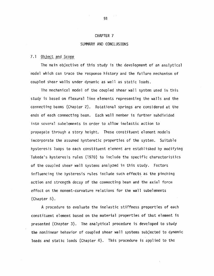
91

CHAPTER 7

SUMMARY AND CONCLUSIONS

7.1 Object and Scope

The main objective of this study is the development of an analytical

model which can trace the response history and the failure mechanism of

coupled shear walls under dynamic as well as static loads.

The mechanical model of the coupled shear wall system used in· this

study is based on flexural line elements representing the walls and the

connecting beams (Chapter 2). Rotational springs are considered at the

ends of each connecting beam. Each wall member is further subdivided

into several subelements in order to allow inelastic action to

propagate through a story height. These constituent element models

incorporate the assumed hysteretic properties of the system. Suitable

hysteresis loops to each constituent element are established by modifying

Takeda's hysteresis rules (1970) to include the specific characteristics

of the coupled shear wall systems analyzed in this study. Factors

influencing the hysteresis rules include such effects as the pinching

action and strength decay of the connecting beam and the axial force

effect on the moment-curvature relations for the wall subelements

(Chapter 5).

A procedure to evaluate the inelastic stiffness properties of each

constituent element based on the material properties of that element is

presented (Chapter 3). The analytical procedure is developed to study

the nonlinear behavior of coupled shear wall systems subjected to dynamic

loads and static loads (Chapter 4). This procedure is applied to the

92

ten-story coupled shear wall models tested by Aristizabal-Ochoa (1976).

These model structures are analyzed for static loads as well as dynamic

loads and are compared with the test results (Chapter 6). The effects

of various assumed analytica') conditions on the maximum responses and

the response waveforms of the model structure subjected to dynamic loads

are discussed (Chapter 6).

7.2 Conclusions

(a) Conclusions Related to the Static Analysesof the Model Structure

The nonlinear structura"' behavior and failure mechanism of structure-l

subjected to static loads which are distributed over the height of the

structure in accordance with the first mode shape are analyzed in

Section 6.2.

The following statements summarize the conclusions made from the

static analysis of structure-l.

(1) The inelastic action of the connecting beams occurs prior

to that of the walls. Yielding of the connecting beams is initiated in

the intermediate levels and then propagates to the upper and lower levels.

(2) It is necessary to assume the form of the axial inelastic

rigidity in the wall section in order to reproduce the overall structural

behavior observed in the test. The use of the reduced elastic axial

rigidity in the wall section, in which the effect of inelastic axial

rigidity is averaged over the height of the wall as well as over the

compression and tension walls, produces a good comparison with the case

which fully includes the effect of inelastic axial rigidity.

93

(3) A large portion of the shear in the tension wall is

transferred to the compression wall due to the early initiation of

inelastic action in the tension wall prior to any development in the

compression wall. This results in only 28% of the total shear at the

base being distributed to the tension wall at the time of initiation

of wall yielding.

(4) The coupling between the walls exerts a considerable

influence on the horizontal displacements and on the base moment. For

example 30% of the total horizontal displacement of the top story is

caused by coupling action when the top displacement reaches a level of

1.75 in. Also 55% of the total base moment is shared by the coupling

moment at the time of initiation of wall yielding.

(5) The flexural moment of the wall is concentrated in the

compression wall reflecting the early deterioration of stiffness

properties of the tension wall prior to those of the compression wall.

This occurs in such a way that only approximately 20% of the total

flexural moment is contributed by the tension wall during the final

stages of loading.

(6) Pinching action and strength decay of the connecting

beams produce larger displacements of the structure in subsequent cycles

and consequently accelerate the deterioration of the structural stiffness.

(b) Conclusions Related to the Dynamic Analysesof the Model Structures

The nonlinear response histories of the model structures, structure-l

and structure-2, subjected to the strong base motions have been analyzed

assuming various analytical conditions and are compared with the test

94

results in Sections 6.3 through 6.6. Structure-2 has relatively much

stronger connecting beams than does structure-l but also is subjected to

stronger base motion than structure-l.

The following statements summarize the conclusions made from the

dynami c ana lyses of structure·-l and structure-2.

(1) Mode shapes of the structures have not changed significantly

during the dynamic motion. Frequencies of the structure have decreased

considerably reflecting the significant reduction of structural stiffness

during the dynamic motion.

(2) The analytical models for structure-l satisfactorily

reproduce the maximum responses and the response waveforms, especially

the elongation of the period due to the deterioration of structural

stiffness, that were recorded during the test.

(3) Comparison of the calculated response of structure-2 with

that of the test is not as good as is the case for structure-l because

the combination of moment and axial force lies outside the limits set

when developing the analytical model. The analytical model cannot properly

treat the crushing of concrete at the base of wall as observed in the test.

(4) Inelastic actions of the connecting beams playa major role

in controlling the structural response since the beam strength controls

the axial forces that develop in the wall, and the wall moment capacity

is affected by the changes of these axial forces in the walls.

(5) The members of structure-2 are more severely damaged than

are those of structure-l because of a stronger base motion applied to

structure-2. The damage is concentrated more at the base of the wall

95

than in the connecting beams for structure-2. The damage occurs mainly

in the connectihg beams for the case of structure-l reflecting the weaker

connecting beam used for structure-l.

(6) Inelastic action of the connecting beams occurs prior to

any such action in the walls. Yielding of the connecting beams starts at

the intermediate levels, then propagates to the upper and lower levels as

observed in the case of static loads.

(7) The response waveform of base shear is governed by the

first mode component but with some influence of the second mode component.

The response waveforms of base moment and displacement are smooth and are

governed by the first mode component. The response waveforms of

acceleration contain higher mode components, especially those for the

lower levels.

(8) The response waveforms of internal forces, such as the

flexural moments of the connecting beams, the total flexural moment at

the base of the two walls and the axial force in the wall at the base,

are governed by the first mode component.

(9) There are fairly large coupling effects between the two

walls. These have a major influence on the base moment and top displace

ment in the dynamic response. For example, 50% of the base moment and

32% of the top displacement are caused by the coupling action of the two

walls at the last peak of the response waveforms. The coupling effect

on the base moment decreases during the dynamic motion primarily due to

inelastic action in the connecting beams. The coupling effect on the top

displacement also reduces during the dynamic motion. This is partly the

96

result of increased wall contribution due to the deterioration of the

flexural stiffness properties of the wall while the decay of the

connecting beam strength holds the couple forces down.

(10) It is necessary to include the effects of inelastic axial

rigidity of the wall section and pinching action and strength decay of

the connecting beams in the calculations in order to reproduce the maximum

displacement response and the elongation of the period that were evident

at the end of the tests. The strength decay has a larger effect on the

maximum displacememt response and on the elongation of the period than

does any pinching action. To assume the reduced elastic axial rigidity

in the wall section is a simple way to include the effect of inelastic

axial rigidity of the wall section.

(11) The use of different numerical integration schemes shows

no significant effect on either the maximum or the waveforms in the

dynamic response even though significant inelastic action is involved.

(12) The use of the updated stiffness matrix for the calculation

of the damping matrix increases slightly the inelastic actions of the

structure during the dynamic motion as compared to the case where the

initial stiffness matrix is used.

(13) To use the coarse arrangement of wall subelements

produces a slightly larger dynamic response of strucrure~l in comparison

to the case with the fine arrangement.

97

LIST OF REFERENCES

1. Abrams, D. P. and M. A. Sozen, "Measured Hysteresis Relationshipsfor Small-Scale Beams," Structural Research Series, No. 432,University of Illinois, Urbana, November 1976.

2. Aoyama, H. and T. Sugano, "A Generalized Inelastic Analysis ofReinforced Concrete Structures Based on the Tests of Members,"Recent Researches of Structural Mechanics, Contributions in Honorof the 60th Birthday of Prof. Y. Tsuboi, Uno Shoten, Tokyo, Japan,1968, pp.15-30.

3. Aristizabal-Ochoa, J. D., "Behavior of Ten-Story Reinforced ConcreteWalls Subjected to Earthquake Motions," Ph.D. Thesis, University ofIllinois at Urbana-Champaign, 1976.

4. Bathe, K. J. and E. L. Wilson, "Stability and Accuracy Analysis ofDirect Integration Methods," Earthquake Engineering and StructuralDynamics, Vol. 1, No.3, January-March 1973, pp. 283-291.

5. Beck, H., "Contribution to the Analysis of Coupled Shear Walls,"Journal of the American Concrete Institute, Proceedings, Vol. 59,No.8, August 1962, pp. 1055-1069.

6. Belytschko, T., "A Survey of Numerical Methods and Computer Programsfor Dynamic Structural Analysis," Nuclear Engineering and Design,Vol. 37, No.1, April 1976, pp. 23-34.

7. Belytschko, T. and D. F. Schoeberle,"On the Unconditional Stabilityof an Implicit Algorithm for Nonlinear Structural Dynamics,"Transactions of the ASME, Journal of Applied Mechanics, December1975, pp. 865-869.

8. Clough, R. W. and K. L. Benuska, "Nonlinear Earthquake Behavior ofTall Buildings," Journal of the Engineering Mechanics Division,ASCE, Vol. 93, No. EM3, June 1967, pp. 129-146.

9. Clough, R. W., K. L. Benuska, and E. L. ~Jilson, "Inelastic EarthquakeResponse of Tall Buildings," Proceedings of Third World Conferenceon Earthquake Engineering, Vol. 2, Session 2, New Zealand, 1965,pp. 68-84.

10. Clough, R. W. and J. Penzien, VynamiC6 06 stnu~~, McGraw-Hill,1975.

11. Coull, A. and R. D. Puri, "Analysis of Pierced Shear Walls," Journalof the Structural Division, ASCE, Vol. 94, No. ST1, January 1968,pp. 71-82.

98

12. Giberson, M. F., liThe Response of Nonlinear Multi-Story StructuresSubjected to Earthquake Excitation," Earthquake Engineering ResearchLaboratory, California Institute of Technology, Pasadena, 1967.

13. Girijavallabhan, C. V., "Analysis of Shear Walls with Openings,"Journal of the Structura'J Division, ASCE, Vol. 95, No. ST10,Oct. 1969, pp. 2093-2103.

14. Goel, S. C. and G. V. Berg, "Inelastic Earthquake Response of TallSteel Frames," Journal of the Structural Division, ASCE, Vol. 94,No. ST8, August 1968, pp. 1907-1934.

15. Hsu, L. W., "Behavior of Multi-story Reinforced Concrete Wallsduring Earthquakes," Ph.D. Thesis, University of Illinois at UrbanaChampaign, 1974.

16. Jennings, P. C., "Earthquake Response of a Yielding Structure,1IJournal of the Engineering Mechanics Division, ASCE, Vol. 91,No. EM4, August 1965, pp. 41-68.

17. Mahin, S. A. and V. V. Bertero, "Nonlinear Seismic Response of aCoupled Wall System," Journal of the Structural Division, ASCE,Vol. 102, No. ST9, September 1976, pp. 1759-1780.

18. Nayar, K. K. and A. Coull, "Elasto-plastic Analysis of Coupled ShearWalls," Journal of the Structural Division, ASCE, Vol. 102, No. 5T9,September 1976, pp. 1845-1860.

19. Otani, S., "Behavior of Multi-story Reinforced Concrete Frames duringEarthquakes," Ph.D. Thesis, University of Illinois at Urbana-Champaign,1972.

20. Paulay, 1., "An Elasto-P1astic Analysis of Coupled Shear Walls,.,Journal of the American Concrete Institute, Proceedings, Vol. 67,No. 11, November 1970, pp. 915-922.

21. Paulay, 1. and A. R. Santhakumar, "Ductile Behavior of Coupled ShearWall"· Journal of the Structural Division, ASCE, Vol. 102, No. STl,January 1976, pp. 93-108.

22. Penzien, J., "Dynamic Response of Elasto-Plastic Frames," Journal ofthe Structural Division, ASCE, Vol. 86, No. ST7, July 1960, pp. 81-94.

23. Rosman, R., IIApproximate Analysis of Shear Walls Subjected to LateralLoads,1I Journal of the American Concrete Institute, Proceedings,Vol. 61, No.6, Part-l, June 1964, pp. 717-732.

24. Sozen, M. A., IIHysteresis in Structural Elements," Applied Mechanicsin Earthquake Engineering, ASME, AMD-Vol. 8, November 1974, pp. 63-98.

99

25. Suko, M. and P. F. Adams, "Dynamic Analysis of Multibay MultistoryFrames," Journal of the Structural Division, ASCE, Vol. 97, No. ST10,October 1971, pp. 2519-2533.

26. Takeda, T., M. A. Sozen, and N. N. Nielsen, "Reinforced ConcreteResponse to Simulated Earthquakes," Journal of the StructuralDivision, ASCE, Vol. 96, No. ST12, December 1970, pp. 2557-2573.

27. Takizawa, H., "Strong Motion Response Analysis of Reinforced ConcreteBuildings (in Japanese)," Concrete Journal, Japan National Council onConcrete, JANACC, Vol. 11, No.2, Feb. 1973, pp. 10-21.

28. Tso, W. K. and H. B. Chan, "Dynamic Analysis of Plane Coupled ShearWalls,1I Journal of the Engineering Mechanics Division, ASCE, Vol. 97,No. EM1, February 1971, pp. 33-48.

29. Tung, T. P. and N. M. Newmark, "A Review of Numerical IntegrationMethods for Dynamic Response of Structures," Technical Report toOffice of Naval Research, Structural Research Series No. 69,University of Illinois, Urbana, March 1954.

30. Umemura, H., H. Aoyama, and H. Takizawa, "Analysis of the Behavior ofReinforced Concrete Structures during Strong Earthquake Based onEmpirical Estimation of Inelastic Restoring Force Characteristics ofMembers," Proceedings of Fifth World Conference on EarthquakeEngineering, Vol. 2, Section 6B, Rome, 1974, pp. 2201-2210.

31. Wen, R. K. and J. G. Jansen, IIDynamic Analysis of Elasto-InelasticFrames," Proceedings of Third World Conference on Earthquake Engineering,Vol. 2, Session 2, New Zealand, 1965, pp. 713-729.

32. Wight, J. K. and M. A. Sozen, II Strength Decay of Reinforced ConcreteColumns,11 Journal of the Structural Division, ASCE, Vol. 101, No. ST5,May 1975, pp. 1053-1065.

33. Yoshioka, K., T. Takeda, and K. Nakagawa, IIInelastic EarthquakeResponse of Reinforced Concrete Buildings,1I Proceedings of FifthWorld Conference on Earthquake Engineering, Vol. 2, Session 6B,Rome, 1974, pp. 2172-2181.

34. Yuzugullu, O. and W. C. Schnobrich, "Finite Element Approach for thePrediction of Inelastic Behavior of Shear Wall-Frame Systems,"Structural Research Series, No. 386, University of Illinois, Urbana,May 1972.

100

Table 6.1 Assumed Material Properties

Properties

Concrete

Compressive Strength f~, ksiTensi1~ Strength f t , ksi

Strain at f~

Strain at f t

Steel Reinforcement

Young1s Modulus, ksiYield Stress fy ' ksiUltimate Stress f u' ksiYield Strain t:..yStrain Hardening Strain t:..hUltimate Strain t:.. u

4.50.403

0.003

0.00013

29,000

72

83

0.00248

O.Ol0.08

101

Table 6.2 Stiffness Properties of Constituent Elements

Structure-l Structure-2

l~a11 Sube1ement

Elastic Axial Rigidity, kip

Elastic Shear Rigidity, kipMoment-Curvature Relationshipof Level 6 to 10 (Primary Curve)

First Slope, kip-in. 2

Second Slope, kiP-in. 2

Third Slope, kip-in.2

Cracking Moment, kip-in.Yielding Moment, kip-in.

Moment-Curvature Relationshipof Base to. Level 6 (Primary Curve)

First Slope, kip-in. 2

Second Slope, kiP-in. 2

Third Slope, kip-in. 2

Cracking Moment, kip-in.Yielding Moment, kip-in.

Beam Rotational Spring

Moment-Rotation RelationshipFirst Slope, kip-in.Second Slope, kip-in.Third Slope, kip-in.Cracking Moment, kip-in.Yielding Moment, kip-in.

21,000

7,610

85,700

28,500

420

4.5

20.0

85,700

50,500

1,000

6.5

39.0

622127

14

0.15

1.56

21,000

7,610

85,700

50,500

1,000

6.5

39.0

85,700

50,500

1,000

6.5

39.0

810

22015

0.15

2.90

102

Table 6.3 Summary of Assumed Analytical Conditions for Dynamic Runs

General Conditions for All Runs

Damping FactorTime IntervalDuration Time, secNumber of Steps

81 = 0.020.000353.08,600

Types of Structureand Base Motion

Run-1 Structure-lBase Motion -1

Run-2 do

Run-3 do

Run-4 do

Run-5 do

Run-6 do

Run-7 do

Run-8 do

Run-9 do

Run-10 Structure-2Base Motion-2

Effect of N* on EI·** 8 in the,and Effect of ¢*** Newmark 8on EA.**** in Wall Method,Included 1

6"

Not Included do(Elastic Axial Rigidity)Not Included do(Reduced Axial Rigidity)

do 14

do 16"

do do

do do

do do

do do

do do

* N = axial force** Eli = inelastic flexural rigidity

*** ¢ = curvature**** EAi = inelastic axial rigidity

/

103

Table 6.3 (continued)

Stiffness Matrix Arrangement Pinching Strengthfor Calculation of of Wall Action of Decay of

Damping Matrix Subelement Beam Beam

Run-l Current Fine Included Included

Run-2 do do do do

Run-3 do do do do

Run-4 do do do do

Run-5 Initial do do do

Run-6 Current Coarse do do

Run-7 do Fine Not Included do

Run-8 do do Included Not Included

Run-9 do do Not Included do

Run-10 do do Included Included

104

Table 6.4 Mode Shapes and Frequencies of Structure-l

Before Run-l After Run-l

First Second Third First Second ThirdMode Mode Mode Mode Mode Mode

(a) Mode Shape

Level

10 1.44* -0.63 0.31 1.43 -0.65 0.34

9 1. 27 -0.33 0.03 1.27 -0.31 -0.01

8 1. 10 -0.02 -0.21 1.10 0.03 -0.28

7 0.92 0.26 -0.31 0.92 0.31 -0.34

6 0.75 0.48 -0.23 0.74 0.49 -0.19

5 0.57 0.59 -0.01 0.56 0.56 0.07

4 0.41 0.59 0.22 0.39 0.52 0.29

3 0.26 0.48 0.34 0.24 0.40 0.38

2 0.13 0.30 0.29 0.12 0.23 0.30

1 0.04 0.11 0.13 0.03 0.08 0.12

(b) Frequency

Hz 5.0 21 48 2.7 13 32

* Modal participation factors are included in mode shapes.

105

Table 6.5 Maximum Responses of Structure-lin Comparison with Test Results

Test Inelastic Elastic Reduced Elastic

Results Axial Rigidity Axial Rigidity Axial Rigidity(Run-l) (Run-2) (Run-3)

Acceleration, g

Level 10 1.66 1.36 1.35 1.419 1. 12 1.04 1.00 1.058 0.75 0.77 0.81 0.797 0.73 0.73 0.75 0.756 0.85 0.82 0.73 0.87

5 0.86 0.83 0.70 0.854 0.82 0.77 0.66 0.843 0.71 0.66 0.60 0.692 0.57 0.53 0.51 0.53

1 0.47 0.50 0.43 0.45Base 0.41 0.41 0.41 0.41

Displacement, in.

Level 10 1. 16 1.16 0.90 1.11

9 1.00 1.03 0.80 0.988 0.86 0.89 0.70 0.84

7 0.71 0.75 0.60 0.70

6 0.58 0.60 0.49 0.56

5 0.46 0.37 0.43

4 0.32 0.27 0.30

3 0.20 0.17 0.19

2 0.09 0.09 0.09

1 0.03 0.03 0.03

106


Test Inelastic Elastic Reduced ElasticResults Axial Rigidity Ax ia1 Rig idity Axial Ri gi dity

(Run-l) (Run-2) (Run-3)

Shear, kipLevel 9 0.83 0.65 0.65 0.69

8 1.37 1. 21 1.17 1. 237 1. 69 1. 67 1. 52 1.576 1.88 1.85 1.72 1. 785 1. 91 1.94 1.85 1.884 1. 94 2.08 2.01 1.893 2.12 2.26 2.22 2.102 2.15 2.31 2.40 2.291 2.37 2.73 2.57 2.47

Base 2.54 2.92 2.71 2.60

Moment, kip-in.Level 9 7.5 5.9 5.9 6.2

8 19.9 16.6 16.4 17.27 34.6 30.4 30.0 31.36 51. 5 45.3 45.3 47.05 69.2 61.8 60.6 63.34 86.0 78.4 76.8 79.73 102.1 91.4 93.1 94.92 118.9 109.7 110.9 108.51 135.4 126.9 128.8 121 .7

Base 151. 5 148.0 148.5 140.6

Frequency, HzBefore Run

1st Mode 4.8 5.0 5.0 4.32nd Mode 20.0 21. 2 21. 2 20.1

After Run1st Mode 2.7 2.7 3.0 2.7

2nd Mode 13.0 13.2 13.6 13.6

107

Table 6.6 Effect of the Numerical Integration Schemeon the Maximum Responses of Structure-1

13* of 1 (3 of 1 1 (3 of 16 4 13 of 6" 4

(Run-3) (Run-4) (Run-3) (Run-4)

Acceleration, g Shear, kipLevel 10 1.41 1.41 Level 9 0.69 0.69

9 1.05 1.05 8 1.23 1.238 0.79 0.79 7 1. 57 1.577 0.75 0.74 6 1. 78 1. 786 0.87 0.87 5 1.88 1.88

5 0.85 0.85 4 1.89 1. 904 0.84 0.84 3 2.10 2.123 0.69 0.69 2 2.29 2.322 0.53 0.53 1 2.47 2.511 0.45 0.45 Base 2.60 2.60

Base 0.41 0.41

Displacement, in. Moment, kip-in.Level 10 1. 11 1.10 level 9 6.2 6.2

9 0.98 0.97 8 17 .2 17 .2

8 0.84 0.83 7 31.3 31.3

7 0.70 0.70 6 47.0 47.0

6 0.56 0.56 5 63.3 63.3

5 0.43 0.43 4 79.7 79.7

4 0.30 0.30 3 94.9 94.9

3 0.19 0.19 2 108.5 108.5

2 0.09 0.09 1 121. 7 121. 7

1 0.03 0.03 Base 140.6 141.3

Frequency, Hz Before Run 1st Mode 4.3 4.3

2nd Mode 20.1 20.1

After Run 1st Mode 2.7 2.7

2nd Mode 13.6 13.6

* The constant of 13 in the Newmark 13 Method.

108

Table 6.7 Effect of the Choice of Stiffness Matrixfor the Calculation of Damping Matrixon the Maximum Responses of Structure-l

Updated Initial Updated InitialStiffness Stiffness Stiffness StiffnessMatrix Matrix Matrix Matrix(Run-3) (Run-5 ) (Run-3) (Run-5)

Acceleration, g Shear, kipLevel 10 1. 41 1.33 Level 9 0.69 0.67

9 1.05 1.04 8 1.23 1.178 0.79 0.78 7 1.57 1.547 0.75 0.72 6 1. 78 1. 796 0.87 0.77 5 1.88 1.875 0.85 0.79 4 1.89 1.934 0.84 0.77 3 2.10 2.203 0.69 0.64 2 2.29 2.452 0.53 0.52 1 2.47 2.611. 0.45 0.44 Base 2.60 2.72

Base 0.41 0.41

Displacement, in. Moment, kip-in.Level 10 1.11 1.03 Level 9 6.2 6.0

9 0.98 0.92 8 17.2 16.68 0.84 0.80 7 31.3 30.27 0.70 0.68 6 47.0 46.16 0.56 0.55 5 63.3 62.85 0.43 0.43 4 79.7 79.04 0.30 0.31 3 94.9 94.03 0.19 0.19 2 108.5 107.62 0.09 0.10 1 121. 7 122.31 0.03 0.03 Base 140.6 145.2

Frequency, Hz Before Run 1st Mode 4.3 4.32nd Mode 20.1 20.1

After Run 1st Mode 2.7 2.82nd Mode 13.6 13.8

109

Table 6.8 Effect of the Arrangement of Wall Sube1ementson the Maximum Responses of Structure-1

Fine Coarse Fine CoarseArrangement Arrangement Arrangement Arrangement

(Run-3) (Run-6) (Run-3) (Run-6)

Acceleration, g Shear, kipLevel 10 1.41 1.42 Level 9 0.69 0.70

9 1.05 1.06 8 1. 23 1.258 0.79 0.78 7 1.57 1. 597 0.75 0.76 6 1. 78 1. 796 0.87 0.87 5 1.88 1.895 0.85 0.85 4 1.89 1. 914 0.84 0.80 3 2.10 2.07

3 0.69 0.69 2 2.29 2.28

2 0.53 0.53 1 2.47 2.481 0.45 0.45 Base 2.60 2.64

Base 0.41 0.41

Displacement, in. Moment, kip-in.

Level 10 1.11 1. 17 Level 9 6.2 6.39 0.98 1.03 8 17.2 17.4

8 0.84 0.88 7 31.3 31. 7

7 0.70 0.73 6 47.0 47.6

6 0.56 0.58 5 63.3 64.35 0.43 0.44 4 79.7 80.7

4 0.30 0.31 3 94.9 96.0

3 0.19 0.19 2 108.5 109.5

2 0.09 0.10 1 121.7 123.1

1 0.03 , 0.03 Base 140.6 140.8

Frequency, Hz Before Run 1st Mode 4.3 4.3

2nd Mode 20.1 20.1


2nd Mode 13.6 13.4

110

Table 6.9 Effects of the Pinching Action and Strength Decayof Beams on the Maximum Responses of Structure-l

Both. Effects Only Strength Only Pinching Both EffectsIncluded Decay Included Action Included Not Included(Run-3) (Run-7) (Run-8) (Run-9)

Acceleration, g

Level 10 1. 41 1.40 1. 41 1.409 1.05 1.05 1.05 1.058 0.79 0.78 0.79 0.787 0.75 0.73 0.73 0.736 0.87 0.85 0.83 0.845 0.85 0.83 0.86 0.874 0.84 0.80 0.84 0.813 0.69 0.66 0.69 0.682 0.53 0.54 0.54 0.531 0.45 0.45 0.46 0.45

Base 0.41 0.41 0.41 0.41

Displacement, in.Level 10 1. 11 1.01 0.89 0.88

9 0.98 0.90 0.78 0.788 0.84 0.79 0.67 0.67

7 0.70 0.67 0.56 0.566 0.56 0.55 0.44 0.455 0.43 0.43 0.34 0.34

4 0.30 0.30 0.24 0.243 0.19 0.19 0.16 0.162 0.09 0.10 0.08 0.081 0.03 0.03 0.02 0.02

11]


Both Effects Only Strength Only Pinching Both EffectsIncluded Decay Included Action Included Not Included(Run-3) (Run-7) (Run-8) (Run-9)

Shear, kip

Level 9 0.69 0.68 0.69 0.68

8 1. 23 1. 22 1.23 1. 22

7 1.57 1. 58 1. 57 1.58

6 1. 78 1.80 1. 78 1.805 1.88 1.89 1.88 1.89

4 1.89 1. 93 1.88 1. 90

3 2.10 2.19 2.17 2.14

2 2.29 2.43 2.53 2.49

1 2.47 2.60 2.77 2.73

Base 2.60 2.70 2.92 2.88

Moment. kip-in.

Level 9 6.2 6.1 6.2 6.1

8 17.2 17. 1 17.2 17.1

7 31. 3 31.1 31.3 31. 1

6 47.0 47.0 47.0 47.0

5 63.3 63.5 63.3 63.5

4 79.7 80.2 79.7 80.2

3 94.9 95.7 94.9· 95.7

2 108.5 110. 1 108.5 110.1

1 121. 7 124.4 121. 7 124.4

Base 140.6 145.2 140.8 141.1

Frequency. HzBefore Run

1st Mode 4.3 4.3 4.3 4.3

2nd Mode 20.1 20.1 20.1 20.1

After Run1st Mode 2.7 2.9 3.3 3.3

2nd Mode 13.6 13.9 14.5 14.5

112

Table 6.10 Mode Shapes and Frequencies of Structure-2

Before Run-l0 After Run-l0

First Seconq Third First Second ThirdMode Mode Mode Mode Mode Mode

(a) Mode ShapeLevel

10 1.46* -0.66 0.32 1.43 -0.63 0.31

9 1.27 -0.32 0.02 1.28 -0.33 0.03

8 1.08 0.02 -0.23 1. 12 -0.04 -0.20

7 0.89 0.31 -0.32 0.96 0.22 -0.29

6 0.70 0.52 -0.23 0.79 0.42 -0.23

5 0.53 0.63 0.00 0.63 0.54 -0.05

4 0.37 0.61 0.24 0.47 0.56 0.17

3 0.22 0.49 0.36 0.31 0.49 0.32

2 0.11 0.30 0.31 0.18 0.33 0.31

1 0.03 0.11 0.14 0.07 0.15 0.17

(b) Frequency

Hz 4.4 21 48 2.5 12 31

* Modal participation factors are included in mode shapes.

113

Table 6.11 Maximum Responses of Structure-2in Comparison with Test Results

Test Calculated Test CalculatedResults Results Results Results

(Run-10) (Run-10)

Acceleration, 9 Shear, ki pLevel 10 1.84 2.22 Level 9 0.92 1.28

9 1. 24 1.71 8 1.52 1. 968 1.00 1.30 7 1.84 2.597 1.10 1.12 6 2.14 2.936 1. 31 1.32 5 2.43 3.105 1. 27 1.43 4 2.72 3.234 1.19 1.41 3 2.97 3.403 1. 10 1. 27 2 3.42 4.002 1.00 0.98 1 3.74 4.441 0.94 0.89 Base 3.92 4.54

Base 0.91 0.91

Displacement, in. Moment, kip-in.Level 10 2.05 1.97 Level 9 8.4 11. 5

9 1.92 1.78 8 22.2 26.5

8 1.69 1.58 7 38.8 49.7

7 1.43 1.37 6 56.2 76.0

6 1.18 1.14 5 77 .6 103.55 0.94 0.92 4 99.8 131.4

4 0.71 0.69 3 121.9 158.1

3 0.50 0.47 2 149.0 185.3

2 0.28 0.27 1 174.9 211.4

1 0.13 0.11 Base 199.1 234.3

Frequency, Hz Before Run 1st Mode 4.5 4.42nd Mode 19.0 20.8


2nd Mode 12.0 12.0

114

o f);Xy

oo

FIXED

II

-oen

~

/v FLEXIBLE. ~ ,..--.V

O V-RIGID~,/'

1--C>--<>-oG"I

O V-ROTATIONAL SPRING

V/

"0-0

,. " WALL ELEMENT

,-- ---..J •• D~(....V-_-----,

AT BASEJ

Fig. 2.1 Mechanical Model of Coupled Shear Wall System

115

RigidLink

FlexibleElement

Springs

RigidLink

Wall Center Wall Center

Fig. 2.2 Connecting Beam Model

>--+-Subelements

II

Wall Center Wall Face

Fig. 2.3 Wall Member Model

5

4en~

en 3enQ)~-(J)

2

0)(

<t

0

116

o 2

Strain x 103

3 4

Fig. 3.1 Idealized Stress-Strain Relationship of Concrete

100 • • • I T

80 -en~ I

en 60 I- -en

'Q)~-(J) 40 I-

Q)

en 20 -c .{!!.

00I I I I I I I I

2 3 4 5 6 7 8 9

Strai n x 102

Fig. 3.2 Idealized Stress-Strain Relationship of Reinforcement

As fs

o

r b -II I

®

~

d'

d

fc

1 I

- As f s

- N

--'--''-J

(a) Cross Section (b) Strain Distribution (c) Force Distribution

Fig. 3.3 Distributions of Stress and Strain over a Cross Section

118

60r------r-----..,.-----r-----~----__,

50

"fi

C = 0.004"c

p=2.0I 40a. "~

p=O- "c

~Q)

E0 30 p=-2.0 "~

OlC P = - 4.0"0C<I>

CD20

• Cracking Point

o Yielding Point

P ( +) Compression

P{ -) Tension

Structure - I

From Base To Level 6

0;50.40,3O'- ..L- ..J.. ...J... --L ......J

o 0, I 0.2

Curvature x 102

J I/in.

Fig. 3.4 Moment-Curvature Relationships of a Wall Member Section

119

2.0,.....-----.,..-----"T-----~----- ......

c

IQ.

...3l:

-cQ)

Eo~

C'C

"CCQ)

(Xl

YieldingEC =0.004

Structure - I

Curvature

°o~------:!-:-----~~----.....I........----.....J0.5 1.0 1.5 2.0

2 .X 10 t I lin.

Fig. 3.5 Moment-Curvature Relationshipof a Connecting Beam Section

120

60r-----..,.-------,.-----r-----...,..-::::---......

Structure --IFrom Base To Level 6

C

Ia.

oXA-c

Q)

Eo~

01.S:"0CQ)

CD

M-rp Curve for a ChangingAxial Load

50

40

30

20

10

p:: 4.0

p :: 2.0

p:: 0

p:: -2.0

p= -4.0

p (+) Compression

p ( -) Tension

0.250.20

O ...... ......r. "-- ...... _

o 0.05 0.10 0.15

Curvaturve x 102

t 1/ in.

Fig. 3.6 Idealized Moment-Curvature Relationshipsof a Wall Member Section

121

2.0r------""T'------,....~----...,..-----_..

c:

c:Q)

Eo~

0.25 4>'1 0.50

Structure - I

0.75 1.00

Fig. 3.7

Curvature x 102

J I / in.

Idealized Moment-Curvature Relationshipof a Connecting Beam Section

L

122

-I. 6L-l

u

•••~•••••""••••••_~Asfs(Tension)

------....--- d'

Fig. 3.8 Bond Slip Mechanism

d

123

2.0,...-...,.--oor--....,.--..,..-.....,,....-.....--_-_

,My '"1.5 '"~

~

/

c: //

I /0- /~ r--Test Result

/1.0 ,-c: /

Q)/E

0 /~ ,C'

/c: /.-

"C0.5 /c:

Q) /m /,,,

Me II

00 2 3 4 5 6 7 8

Rotation x 103

rod.J

Fig. 3.9 Idealized Moment-Rotation Relationshipof a Rotational Spring

124

Upper End

Fig. 4.1

Lower End

L

Force and Displacement Componentsat Wall Member Ends

Upper End Lower End

Ps I Us

C D B f2 3

-NBIVB

~MB

1·8B

t 11 .... t2 -+- h

JL

Fig. 4.2 Cantilever Beam withThree Subelements

12,5

/ IRotational Springs

A C 0 B

I~.. 8.

e 0

l./M. ,8.NA I VA Ne 'Ve

fa >.L ~. L .-t->.L

-tRigid Flexible RigidLink Element Link

Fig. 4.3 Force and Displacement Componentsat Connecting Beam Ends

Fig. 4.4 Moment Distribution of aConnecting Beam

126

C D-----:0 0

Initial Position

B

__xL__•1

.....__L • ~~_X_L 'I

Fig. 4.5 Deformed Configurationof a Connecting Beam

127

cCDEo~ Primary curve..:\. __

----

Deflection

Fi g. 5.1 Takeda's Hysteresis Loops

Nco

COMPRESSION

M

My { f/!£-~_

p= 3.0p= 2.0

~p: \.0

=- ~: ?\.O

» , ; ep

TENSION

Fig. 5.2 Hysteresis Loops with Effectof Changing Axia1 Force

~

N~

[:~~RY CURVE___--7j-

My

M

My

--

---- rGUIDELINE FOR-- -t:. DECAY OF BEAM

STRENGTH____-,.olIIIIiEiIi:::~=-'~L .8

7 ~

Fig. 5.3 Hysteresis Loops with Effects ofPinching Action and Strength Decay

All Flexural Reinforcement!No.8 Gage WireAs = 0.0206 in.2

130

I0.34

I 0 0 0 01.0 0.320.34

0 0 0 0

~ 7.0 ~Wall Flexural Reinforcement From Base To Level 6

I0.34

I 0 01.0 0.32

0 00.34

E:J 7.0 ~Wall Flexural Reinforcement From Level 6 To 10

1.5 ~:;:~CJ0.25~ 0

~Beam Flexural Reinforcement

(a) Structure-I

I.~ ~II-_g_g g__g_

1,-:·_~_..Q_~I 7.,-,-0 ~Wall Flexural Reinforcement For Full Height

1.5

0.25

1.00

All Flexural Reinforcement:No.8 Gage Wire

As = 0.0206 in.2

Fig. 6.1

(b) Structure - 2

(Dimensions In Inches)

Cross-Sectional Properties of Wall and Beam

131

CompressionTension

@c ~~ ~~l~c- - - - - - - --~-53-- - ---~----- 7C 7C -~~---

@57 Y 57 Y

5 C

2

6

5

:3

9

8

7

4

10

Q)

>Q)

-J

...ooLL

SubelementRotationalSpring

o = Number Indicating Time Sequence Of Occurrence

C = Cracking Y = Yielding

Subelement

Fig. 6.2 Sequence of Cracking and Yielding of Structure-lunder Monotonically Increasing Load

--'WN

:3

Dead Load Effect Is Excluded

o Inelastic Axial Rigidity

6 Elastic Axial RigiditySymmetric About Origin

-I 0 1 2

Vertical Displacement At Top Of Wall x 102

, in.

coenc~

~

~coenenIU...a.Eou

4

2

6

8

-8

-8

-2

-6

-4

~

c»~ 01 I Im

-o

o)(

<r

C.

.¥

«c»u...If

Fig. 6.3 Relationship of Base Axial Force and Top Vertical Displacementof Walls of Structure-l under Monotonically Increasing Load

- Beam Yield ing Starts

200

.c

150ICL.-.:rt:..-cCDE 1000:;:CDIn0m

50

Wall Yield ing Sta rts--

--- Wall Cracking Starts

Starts

Results *

o Inelastic Axial Rigidity6 Elastic Axial Rigidityo Reduced Elastic Axial Rigidity

• Pseudo Stat ic Curve Due ToThe First Mode Components OfThe Dynam ic Responses In Test

2 3

--'ww

Top Floor Displacement, in.

Fig. 6.4 Base Moment-Top Displacement Relation of Structure-lunder Monotonically Increasing Load

134

~0 100

c0

01- c::J

~.0 u Compression Wall... 0...- U 01en.~

0 ~

eu... r0Q)

~.cenQ)en

Tension Wall0m

00 3.0

Base Shear Force, kip

Fig. 6.5 Redistribution of Base Shear in Walls of Structure-lunder Monotonically Increasing Load

~100r-----..,..-----~----...,..-----_r_-_..

Beam Cracking

°o~----~~----~----~~---~~-~0.5 1.0 1.5 2.0

A-cQ)

E 80Q)ooQ.eno

o-{!.

--c 0Q) Q)E_~wo 0'Q. Cen

i:5 Q. ...:J 0

... 0 08 U IJ...

iL: {!. Q.

a. Q) {!.~5

Total Top Floor Displacement J in.

Fig. 6.6 . Ratio of Top Displacement due to Coupling Effect toTotal Top Displacement of Structure-lunder Monotonically Increasing Load

135

100

Coupling Moment90

~ Ul

80 -..Ul

Ul Ul CC - - -.. -~ c .. .. (f)

Q) - c c- (f) - - Cl- 70 (f) cJ) c:0a.. Cl

Cl Cl'tJ

c::i: c: c: CIl

C u ...:: 'tJ >=.2 60 c u CIl.. C- U .. >=~ U~ E E~- c c c

50 CIl CIlen CD 3: CD0

- •CQ)

E0:EQ)

Ofen Moment Compression Wall0

CD

Moment Of Tension Wal.1

20018016014012010080604020

o-_......__"'-_--I.__...._.....ir..-_....__"'--_...__""'-_....Io

Bose Moment t kip - in.

Fig. 6.7 Base Moment Distribution Pattern of Structure-lunder Monotonically Increasing Load

136

10

9

8

7

6

...oo

LL5

4

3

2

I I20 kip - in.

Tension Compression

Fig, 6.8 Moment Distribution Patterns in Membersof Structure-1 at the End DfMonotonically Increasing Load

200, ii' i i •

100c,Q..-~.-C 0Q)

E0~

Q)U)

CCD

-\00

"//

/

'"///

//

/ - Pinching Action AndStrength Decay Of Beam

--- No Pinching Action AndSt rength Decay Of Beam

.....W-....l

1.51.00.5-200' I I I I I I

-1.5 -1.0-0.0 U

Top Floor Displacement, in.

Fig. 6.9 Base Moment-Top Displacement Relation ofStructure-l under Cyclic Loading

0.50

0.0

-0,50

l , 00

0,0

-t. 00

138

(0) BASE MOTION - I

(b) BASE MOTION - 2

a 2

TlMe. SEC

Fig. 6.10 Waveforms of Base Accelerations

3

139

10

9

e

7

6Q,)

>j

5~

00

LL 4

3

0 First Mode

2 Ii Second Mode

0 Third Mode

O'"----"-----..L.--__......I...... ..L.. .....-0.5 0 0.5 1.0 1.5

Modal DisPlacement·7(

Modal Participation Factors Are Included In ModalDisplacement

Fig. 6.11 Initial Mode Shapes of Structure-l

140

10

9--0- Calcu lated Result

- ....- Test Result8

7

6Q)

>Q)

...J 5~

00

L1.. 4

3

2

1.0"0,5o1.00.501.-_.......__..1-__&...-_.....__...... ..... &...-_--'

o

Maximum Acceleration, 9 Maximum Displacement, in.

Fig. 6.12 Maximum Responses of Structure-l, Run-l,in Comparison with Test Results

141

200o

10

-0- Calculated

9Result

--e-- Test Result

8

7

Q) 6>Q)

-J

~ 500

LL4

3

2

Maximum Shear, kip Maximum Moment, kip-in.

Fig. 6.12 (continued)

142

~

\\V

\\\

III/~II \

II,

I\I II II I\ I\ I\ I

kl -IN.

1\\I\

III

I ,I II I",'

I '

~I\I

(a 1

I

IIII

IIIII,

- - -TEST RESULTS

IIIII.,

~ I\ I

\J \l( b1 Sf erVEA1UANl NO MOMEN'T,

1--------+1--------+1---------41a I 2 3

TlME. SEC

0.0

~

2.00 III

\II

0,0

100.

-~.oo

-100.

Fig. 6.13 Response Waveforms of Structure-1, Run-1

143

L. 00

£1.0

-\. 00

~

I I Ii' \~I I 1

,I

(C 1 ACCElERA110N Al LEVEL ~ D. (j "

" ~~

l.OO - - - TEST RESULTS

£1.0

-1. 00

(d 1 ACCRERAl ION Ri LEVEl .Q. 0

L. 00

0.0

-1. 00

o

f e 1 RCCREAA110N Ai LEVEL 8. 0

I2

TIMe. SEC


3

l. 00

er.o

-1. 00

l. 00

er.o

-1. 00

l. 00

er.o

-1. 00

144

(f 1 .qCCaERA1!tIN R1 LEVEL 1. G

(9 1 .qCCaERA1HfN .q1 LEVEL 6 I 0

(hl ACCaERA1HfN.q1 Lcva 5. 0

I[J 2

TIME. SEC


3

to 00

0,0

-1. 00

l. 00

0,0

-1. 00

l. 00

0,0

-1. 00

145

f i 1 ACCaERAi JON Al LEVEl 4, G

, j 1 RCCCl..ERRi JON Rl LEVa '3, G

a

f k 1 ACCCl..ERRi urN Al LEVEl ~. 0

I Il 2

TlME, SEC


3

L. 00

0.0

-\, 00

146

r I' ACCaEAA110N Ai LEVEl 1 I 0

l. 00

0.0

-l. 00

--- TEST RESULTSrm, OJSPUICEHENT RT LEVEL 10, IN.

l. 00

0.0

-l. 00

rn, OJSPLACf:HENT AT LEVa ,g. IN.

"'-1--------+---------Ir------------11023

TlME. SEC


1. 00

0.0

-1. 00

1. 00

0.0

-i. 00

1. 00

0.0

-1. 00

147

(01 OJSPLRCeHENl Rl LEVEL 9. IN.

(pl OJSPLRCEHENl Rl LEVEL 1. IN.

a

Iql OJ5PLRCEHENl Al LEVEL 6. IN.

I I1 2

TIME, SEC


1. 00

a.o

-l. 00

LOO

0.0

-1. 00

l. 00

0.0

-\, 00

148

I r l DJSPLACEHENT RT LEVEL 5. IN.

Is l OJ5PLACEHENT AT LEVEL 4. IN.

a

It l OJ SPLACEHENT AT LEVEL '3. IN.

I I1 2

TIME. SET


3

l. 00

[flO

-\. 00

l. 00

[flO

-L.DO

149

ru 1 OJSPUICEHENi Ai LevEL 2 I IN.

a

rv1 OJ 5PLACEHENi Ai LEVEl 1 lIN.

I Il 2

TlMc l SEC


3

l. 00

0,0

-L.OO

150

(0 1 OJ5PLACeMeNl Ai LtvE'L 10. IN.

2.00

0.0

-2.00

LOa.

0,0

- LOa.

o

(b) BRSE SHtRA AcSP8NSE, KIP

(C 1 Sf: erVEA1UANING MOMeNT, kIP-lN.

2

TIMf: I SEC3


151

L. 00

0.0

-t.OO

(a 1 DJSPLAr:EHENT AT LEVEL IU, IN.

3l 2

TIME. SEC

Ie 1 Sf rrVEA1UANING MrJMENT. KIP-lN.

I I

fbl BASE SH£AR RE5P~NSE. KlP

o

0.0

0.0

2.00

-tOO.

-2.00

. tOO.


152

T~P ST.OEFLECTI~N ADD 1ST ST.~.T.M.. x

r-'>

:I:Uz:+-;

I£L........

.::E.t-

O

-1.10 I.lIJ

DEFLECT I~N (l NCHl

Fig. 6.16 Response History of Base Moment-Top DisplacementRelationship of Structure-1, Run-1

2

153

-2

(a) Moment Of Rotational Spring J kip- in.Level - 10

-I

-2

(b) Moment Of Rotational Spring J kip- in.Level -8

I I I I I I0.5 1.0 1.5 2.0 2.5 3.0

Time J sec.

Fig. 6.17 Response Waveforms of Internal Forcesof Structure-l, Run-l

154

2

-2

(c) Moment Of Rotational Spring I kip - in.Level - 6

-2

(d) Moment Of Rotational Spring I kip -in.Level - 3

' 1..... ' __~I---1..._----..110.5 1.0 I. 5 2.0 2.5 3.0

Time I sec.


155

(e) Moment Of Rotational Spring» kip-in.Level - I

75

-25

(1) Total Flexural Moment Of Two Walls AtBase» ki p -i n.

I__--~I__---II~_~I-_-.....I---I0.5 1.0 1.5 2.0 2.5 3.0

Time » sec.


Tension

10

5

-5

-10Compression

156

(g) Axial Force Of Wall At Base. kip

0.5 1.0 1.5 2.0

Time • sec.

2.5 3.0


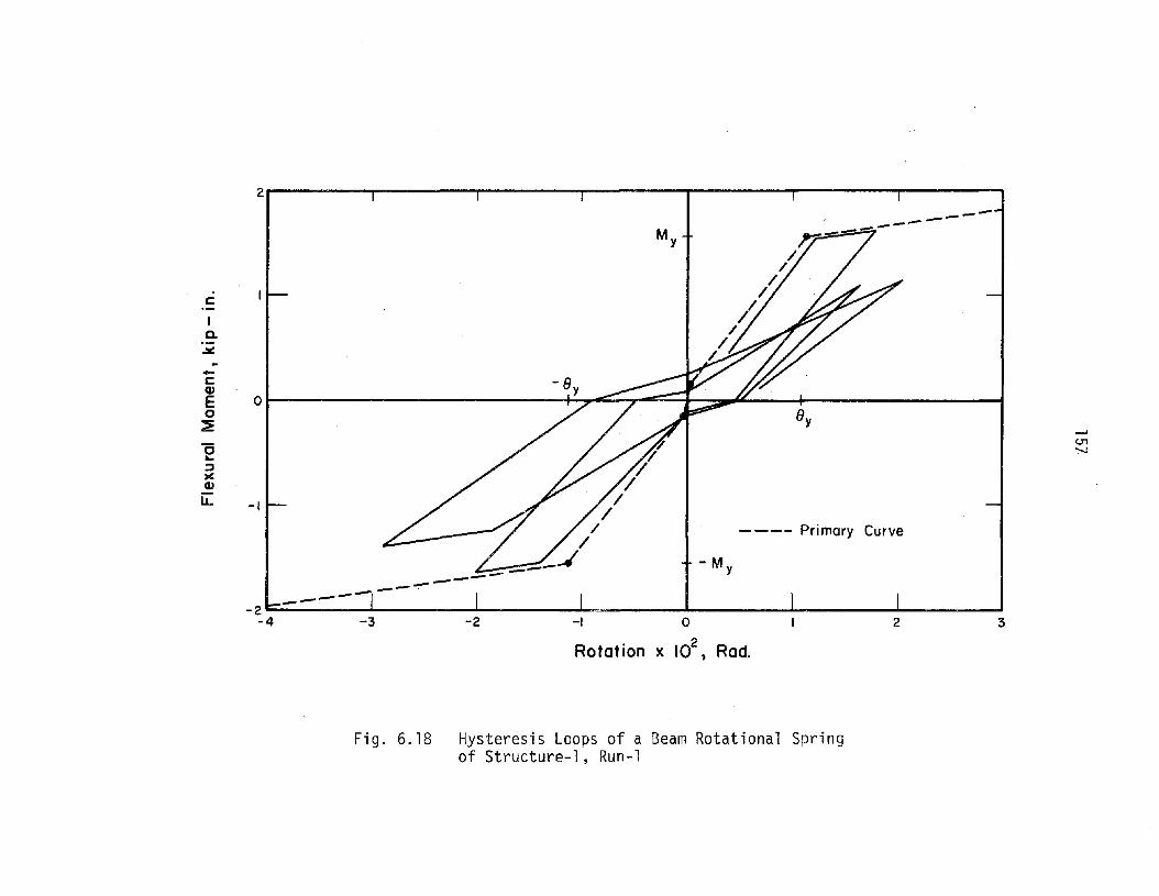
r I ~~_2 _--I __

My

.Lc:

IQ.

~

~-~ °1 / /~ By I i5l.o:::J)(Q)

I.L. -I / // / / I Primary CurveI

-M y

L------r----i L.-.-L I 2 3-2 -2 ~ 0-4 -3 2

Rotation x 10 , Rad.

Fig. 6.18 Hysteresis Loops of a Beam Rotational Springof Structure-l. Run-l

158.

Tension r----/

//

//

//

//

//

//

//

//

//

//

----4

---- Primary Curve

Compression

-60 '--_......L.__...L-_--"__......._---IL...-_...J-__.L.-_.....L__.J-_--1

-10 -8 -6 -4 -2 0 2 4 6 8 10

Curvature x 106

, II in.

Fig. 6.19 Hysteresis Loops of a Wall Sube1ementat Base of Structure-1, Run-1

Q)

>Q)

....J

~

oo

lL.

159

10

@)c @)c@c @)V @v @C

9®=C_-=--==-=@C

@)V @C

~C------

CDc I- -----

@V @C

----RG-=~=~@C @C

@)V @V @C

@C

@C @C4 ------ --- ------

@~------~~ ~~ I--@ ~----@C @C

3 ------- -------@C @C@C---- @C~==~~@)C------ @C

2 ------------------@C IC IC@C------ @V @V --------

@C @C-------, ---------

@C

@C @r

0c <Dc @C

G)c @V

Subelement Rotational SubelementSpring

0= Number Indicating Time Sequence of Occurrence

C =Crocking V = Vielding

Fig. 6.20 Sequence of Cracking and Yielding forDynamic Response of Structure-l, Run-l

100. I I I I ---- T

't!-

- 80L -c: -Q) c:E Q)

0 E 0~ ~ 60 0 0 fQ) 0 0 0 0II)

Q) CJl 00 c::

II)m 0 40 '0 1 --'

m Ql O'l

C' :;:: ac: E::Q. 0 20 o 0::J - Ql ....

0 ~IDC/)

U

0' I I I I l0.25 0.5 1.0 1.5 2.0 2.5 3.0

Time t sec.

Fig. 6.21 Ratio of Coupling Base Moment to TotalBase Moment at Peak Responses ofStructure-l, Run-l

100, iii f , i

~

--'Q).....

-

-

3.0

o

2.5

oo

2.0

o

1.5

o

1.0

oo

0.5

o

01 I I I I I I0.25

601-

801-

0- 401-~

.E 20 ......{2

cQ) Q)

j Eo _ Q)

o 0- Q) 0C __

Q) - 0-E UJ .!!?Q) 0U tJlo CCi=(/) 0-.- j080-

{:.~

Time, sec.

Fig. 6.22 Ratio of Top Displacement due to Coupling Effectto Total Top Displacement at Peak Responsesof Structure-l, Run-l

162

10

9

8

7

SQ)

>Q)

...J5

~

00

U. 4

3

0 Toto I 0 isplocement

2 ~ Displacement Due ToCoupling Effect

o 0.5 1.0 1.5

Displacement, in.

Fig. 6.23 Coupling Effect of Walls on DisplacementDistribution at the Maximum Responseof Structure-l, Run-l

1. 00

0.0

-l. oa

163

. (0' OJ SPLRCfMtN1 A1 LEVEL 1D, 1N.

2.00

0.0

-2.00

lOa.

0.0

-100.

a

fb) BASE SHEAR AE5PefNSf. lOP

( c , Sf rrv fR1UANJ NG MOMENT. IOP-) N.

I2

UME, SEC

3

Fig. 6,24 Response Waveforms of Structure-l, Run-5

1. 00

0.0

-l.OO

164

rol OJSPLRCEI1ENl Rl LEVEL 10, IN,

2.00

0.0

-2.00

lOO,

0,0

-lOO,rCl SE nVER1UANINO MftMEN1. KIP-lN.

11--------1 Ia l 2

TIMt, SEC


3

1. oa

0.0

-L, 00

165

ro) OJ SPLRrEHENl Rl LEva 10, 1N.

2.00

0,0

-2.00

lOa,

0.0

-lOa,

o

rc 1 SE ffVEA1UANINO MOMENl r tOP-lN.

I2

TIME. SEC


3

L. 011

11.0

-t. 03

2.011

11.0

-2.00

1(111 •

166

(a 1 OJSPlACE'ME:Ni Ai LevEL 10, IN.

(b 1 BASE SHEAR AESPffNSE, KlP

0.0

-1011 .

(C 1 SE I7VER1UANINO MrJMEN1, KIP-lN.

~I-------+-------.J-I------_1a 2 3

TIME. SEC


L. 00

0.0

-t. 00

2.00

0.0

-2.00

tao.

167

(0) OJSPLACEI1ENl Al LeveL 10, IN.

( b 1 BRSE' SHEAR AcSP erNSt:: I KlP

0.0

-loa.

(J

(C ) Sf: erVER1UANING MrJMEN1. kIP-lN.

I I1 2

TIME. SeC3

Fig, 6.28 Response Waveforms of Structure-1, Run-9

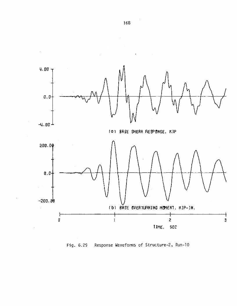
Y.DO

a.D

-4.00

200.

a.D

-200.

168

fa 1 BA SE SHEAR AE SP fJNSE I KJP

rbl BASE fJVEA1UANINO M~EN1, KIP-JN.I I

D' I 2

TlME. SEC


2,00

0.0

-2.00

2,00

0,0

-2.00

2,00

0,0

. -'2.00

169

rc) ACC&EAR1HJN Al LEVEL 10, D

rd 1 ACC&ERRl HJM Rl LEVEL g I 0

(e) ACCaERRl HlN Al LEVEL a I 0

I~------+I-------+-I--------flo 1 2 3

TIME. SEC


2,00

0.0

-2.00

2,00

0.0

-2.00

2.00

0,0

-2.00

170

(f 1 RCCREAR11ffN R1 LEVEL 1 I 0

(g 1 RCCElERR11ffN A1 LEVEL G. 0

Ih 1 RCCElERR1HrN A1 LEVEl 5 I 0

~-------I--------+I---------11

a I 2 3

TIME. SEC


2,00

0,0

-2.00

2.00

0,0

-2.00

2,00

a,o

-2.00

171

r i 1 RCCB-ERRllffN Rl LEVEl LJ, 0

( j 1 RccaEARllftN Ai LEVEl '3 r 0

a

(kl AccaERA1HrN Al LEVEl '2 I 0

I II 2

TIME r SEC


3

2.00

0.0

-2.00

2.00

0.0

-2.00

2.00

0.0

-2.00

172

r, 1 ACCaERA11frN Al LEVEL 1 I 0

rml DJSPLACEMENl Rl LEVEL 10. IN.

(n 1 OJSPLRCEMEJIfT Rl LEVEL .9. IN.

ICJ 2

TlME. SEC


2.0U

0.0

-2.00

2.0U

a,o

-2.00

2.00

O.U

-2.00

173

r 01 DJSPLACEMENl Al LEva 8, IN.

fP1 DJSPlRCEMEN1 Rl LEVEL 1. IN.

a

rql OJSPLRCEI1EN1 Rl LEVEL 6. IN.

I II 2

TIME, SEC


3

2,00

0.0

-2.00

2,00

0.0

-2,00

2,00

0.0

-2.00

174

fr 1 DJ5PLRCEMEN1 ~1 LEVa 5. IN.

__ /\ A 1\ /\~ /

rSl OJSPLACEMEN1 Al LEVa LJ. IN.

a

f t 1 OJ SPLRCEMENl Rl LEVEL '3. 1N.

I I1 2

TlME. SEC


3

2.00

0.0

-2.00

2.00

175

rUl OJ5PLRC€MEN1 Ai LEVa ~. IN.

0.0

-2.00fv 1 OJSPLRCEMENl Ai LEVEL 1. IN.

~I-------t 1--------11a I 2 3

T1ME. SEC


176

10

8

7

9

26 Y

2

3

5

4

6

-.oo

LL

Q)

>Q)

..J

Subelement Ratat iano I Springo = Number Ind icat ing Time Sequence Of Occurrence

C = Crocking Y = Y ieJd ing

Fig. 6.30 Sequence of Cracking and Yielding forDynamic Response of Structure-2, Run-10

177

APPENDIX A

CALCULATIONS OF WALL STIFFNESS PROPERTIESIN THE COMPUTER PROGRAM

The detailed procedure to evaluate the wall stiffness properties in

the computer program is schematically discussed in this appendix. TheaM aM aN aN

properties to be evaluated are a¢' an' aE' and o¢' These quantites are

first defined in Eqs. (3.10) and (3.11) of Section 3.3.

The instantaneous flexural rigidity and axial rigidity of a wall

subelement are derived from these properties as shown in Eq. (3.13) of

Section 3.3. These properties are varied nonlinearly and correlated

mutually in the process of inelastic action of a subelement making the

problem highly complicated.

It is desirable to linearize these properties in a piecewise fashion

for simplicity, because the hysteresis rules are already developed around

a trilinearized version of the primary curve.

A.l Calculation of Pseudo-Flexural Rigidity ~

The procedure to develop an idealized moment-curvature relationship

for a constant axial force is discussed in Section 3.3. The series of

idealized moment-curvature relationships for different values of constant

axial force are shown in Fig. 3.6.

A major difficulty in the calculation of ~~ is that there are an

infinite number of moment-curvature curves corresponding to different axial

forces and axial force variations although the hysteresis rules require

a single moment curvature curve.

178

To avoid this difficulty, a moment-curvature relationship for a

specified axial force is chosen to be the primary curve of the hysteresis

loop. The dead load of the wall is considered as the specified axial

force for which the primary curve is chosen. The primary curve is shown

by the thick solid lines in Fig. A.l.

In an actual loading process, the moment-curvature curve may depart

from this primary curve due to changes in the axial force. In establishing

the various curves the yielding curvature for any moment-curvature curve

is assumed to be the same regardless of axial force level, Fig. A.l.

If the moment, axial force, and previous loading history are known

at a stage in the loading process, the location for the present loading

level can be specified as shown in Fig. A.l.

If the location of the present loading level happens to be at

point A, the referring point Alan the primary curve can be located by

projecting vertically down from point A to the intersection with the .

primary curve as shown in Fig. A.l. The moment at the referring point

A" is calculated from an equation of the form:

(A.l)

where

mAl = moment at the referring point AI

rnA = moment at the point A

~n = difference between the present axial force

and axial force for the primary curve

In this procedure, whether the cracking point or the yielding point

has been exceeded or not can be checked by referring to the hysteresis

(A.2)

179

loop of the primary curve.aM .

The value ~ for an arbitrary moment and axial force can be calculated

by locating the referring point on the hysteresis loop of the primary curve,

then modifying the slope of hysteresis loop at the referring point.a~1The modification of a~ can be expressed as follows:

K= KO~ + 8(~l: -nolJ

where

K = ~~ for arbitrary moment and axial force

KO = ~~ at the referring point on the primary curve

~(~~) = increment of ~~ at the referring point on the primary curve

~m = increment of moment at the referring point on the primary

curve

n = axial force (compression ;s positive)

no = axial force for which the primary curve is evaluated

(usually dead load)

aMA.2 Calculation of ~

The value ~~ can be evaluated by examinating the idealized moment

curvature relationship in Fig. 3.6. For simplicity sake, it is assumed

that ~~ is a linear function of the moment level. The evaluation of ~~

at an arbitrary point on the hysteresis loop is schematically explained

in Fig. A.2.

First, the values of ~~ at specified moment levels of the primary

curve are determined by taking an average of the values ~~ for different

180

axial force levels at each specified point. The levels of zero moment,

cracking moment and yielding moment are chosen as these specified

levels.

The value ~~ is assumed to be zero at the zero moment level.

After the yielding level, the value ~~ is considered to be constant.

The value ~~ at an arbitrary point in the hysteresis loop can be evaluated

by linearly interpolating the values ~~ at specified levels such as the

cracking and yielding levels.

The procedure to evaluate ~~ can be applied to the unloading curve

as well as the loading curve with one exception. The exception to this

procedure is that before cracking is initiated by the loading, the valueaM .an is always zero, taking account of the characteristics of the moment-

curvature relation of the reinforced concrete section.

A.3 Calculation of Pseudo-Axial Rigidity ~

The axial force-axial strain relationship corresponding to a given

curvature can be calculated by using the procedure explained in Section

3.2. In the procedure, the axial strain is determined by taking an

average of the axial strain distribution over the cross section. A

series of axial force-axial strain relationship curves are shown in

Fig. A.3. There are an infinite number of such axial force-axial

strain curves corresponding to different values of curvature.

It is assumed that the relations between axial force, axial strain,

and curvature are kept to be always the same regardless of the loading

history. This means that the deterioration of axial rigidity depends only

on the axial force and curvature. Therefore, if the axial force and

181

curvature at any stage in the loading process are known, the present

location in the loading process can be specified without knowing the

previous history of loading. The slope of the axial force-axial strain

curve at that location is considered as the instantaneous pseudo-axial

rigidity ~~.

To simplify the problem, the axial force-axial strain curve is

slightly modified. In the computer program each axial force-axial strain

curve is represented by a straight line with a different slope as shown

in Fig. A.4.

The variation of the slope ~~ with respect to curvature ¢ can be

expressed approximately by a third order equation in the curvature, ¢,

as shown in Fig. A.5. It is assumed that if a curvature <p exceeds the

limiting value, the value ~~ becomes constant.

The slope, ~~, is expressed as follows:

o 2- I<pI 2- b

~ = a(b - 1¢1)3 + cdE:

(A.3)b < I<pI

aN-= cdE:

where

a, b, and c = coefficient of the third order equation

I¢I = absolute value of curvature

The coefficient a, band c should be evaluated so that the approximate

expression of the ~~ - ¢ curve in Fig. A.5 is made as close to the real

one as possible.

182

The range of axial force-axial strain curves is limited by two

boundary lines A and B as shown in Fig. A.3. If an axial force-axial

strain curve exceeds either boundary line, A or B, the curve is then

assumed to travel along the line A or B depending on which line is

exceeded.

Line A corresponds to the situation when the tensile stress due to

moment is overcome by the compressive stress due to compressive force.

There is no tensile stress on that section. Line B corresponds to a

full cracking stage in which only reinforcing bars exist on a section

after cracking.

Line A can be approximately straight until a concrete crushing is

initiated. Also line B can be straight until reinforcement yielding

happens.

The equation of the idealized axial force-axial strain lines in

Fig. A.4 can be expressed as follows:

Within the range limited by two boundary lines A and B

N = ~ E: + (~) x <PaE: 3<PE:=O

Otherwise (A.4)

N = K1E: (compression)

N = K2£ (tension)

where

N = axial force (function of <p and £)

E: = axial strain

~~ = slope of N -E: line that is defined in Eq. (A.3)

183

(~) = differentiation of axial force with respectdep E=O

to curvature at zero axial strain

cP = curvature

Kl = slope of boundary line A

K2 = slope of boundary line B

A.4 Calculation of ~

The expression of ~~ can be obtained by simply differentiating

Eq. (A.4) with respect to curvature cp.

The results of this differentiation are expressed as follows:

Within the range limited by two boundary lines A and B

Otherwise

where

-b ~ cp ~ 0

cp ~ -b

dN = ddCP

dN - -3a(b _ ~)2 E + ddCP - 'fJ

~~ = 3a(b + cp)2 E - d

dN~ = -d

~:: 0dCP

d :: (~)dCP E=O

(A.5)

M

Fig. A.1

M

Fig. A.2

184

Present Loadinq Point

_-------n4

_-------n3_-------02 {Pri mary Curve}

_-------n,

Primary Curve for HysteresisLoops of a Wall Member Section

_---~- - - - n4

L-~--:7 - - - °2 (Primary Curve)

too = n 4-n2

Evaluation of ~~ for HysteresisLoops of a Wall Member Section

• 4Curvature x, 0 .' lin.

-'co<.n

4

A

2

Compression

o-2-6 -4

Strain x '04

Axial

-6' I K , I I I I I I "

-14 -12 -10 -8

,0 'I , , i:=;SS , :::>" :::;A 7 >' > , I

c)(

<{

cuCo)...If

Q..-.:II:

Fig. A.3 Axial Force-Axial Strain Relationshipof a Wall Member Section

*Curvoture x 104

I 1/ in.

10" i , , :> i >' 51 i>" > I, i

-14 -12 -8 -6 -4 o

Axial Strain x 104

Fig. A.4 Idealized Axial Force-Axial Strain Relationshipof a Wall Member Section

",

'0

2 1"to IQ

Q)

a.o(f)

187

22,----,.--.,...--.....--....,--..,...--,...---,.--...

2 o Slope aN From Fig. A. 4aE

00 2 4 6 8 10 12 14 16

Curvature x 104

Jilin.

Fig. A.5 Relationship of Slope of Axial ForceAxial Strain Line and Curvaturefor a Wall Member Section

188

APPENDIX B

COMPUTER PROGRAM FOR NONLINEAR RESPONSE ANALYSISOF COUPLED SHEAR WALLS

The computer program was developed to calculate nonlinear response

of coupled shear walls under dynamic loads as well as static loads. The

method of analysis was described in Chapter 4. The program is limited to

the analysis of a symmetric coupled shear wall structure with less than 11

stories. A wall member can be divided into subelements in any arrangement

up to 7 elements.

The total core space required to run the program is approximately

220 kilo-bites in IBM 360/75 computer, including temporary disk space for

calculated response values. It took approximately 15 minutes of computing

time to run the program for the nonlinear response analysis of a ten-story

coupled shear wall structure subjected to 3 seconds of base motion at a

.00035 second time interval. Calculated response values were temporarily

stored in disk space and were plotted at the end of analysis on a CALCOMP

plotter.

The flow diagram of the computer program for nonlinear response

analysis of coupled shear walls is shown in Fig. B.l.

189

Start

Read and print:

IStatic case I

1. structural geometry2. unloading coefficients of

hysteresis loops3. stiffness properties of wall

subelements4. stiffness properties of beam

rotational springs

IDynamic case I

Read and print: 1. mass of each story I2. damping coefficien~

Initialize: 1. member stiffness properties2. response values

Compute and print: 1. translation matrices2. initial member stiffness

matrices3. initial structural stiffness

matrix1 ....-- ----'

6Fig, 8.1 Flow Diagram of Computer Program for Nonlinear

Response Analysis of Coupled Shear Walls

190

9~ ~

IStatic case I I Dynamic case I

ICompute and print: 1. initial damping matrix

2. mass matrix3. modal characteristics

of the structure

tIStatic case I IDynami c case I

t L 1Read: 1. stati c loads I Read: l. base accelerationI

record

~I

Step routine start

[ Compute: 1. incremental external forces

case l.

Compute: 1. incremental structural responsesfrom equation of motion

Static case

2 3

Fig. B.1 (continued)

4

191.

2

Compute: 1. incremental structural responsesfrom structural stiffness matrix

Compute: l. total structural responses

2. incremental member end forces anddisplacements

3. total member end forces anddisplacements

4. new member stiffnesses based on currentforce levels and hysteresis rules

5. new structural stiffness matrix

case IStatic IDynami c case I

~

Compute: l. new damping matrix I f nex,Record: 1. maximum and minimum structural responses

2. maximum and minimum member and forces

5

4

t step

6

Fig. B.l (continued)

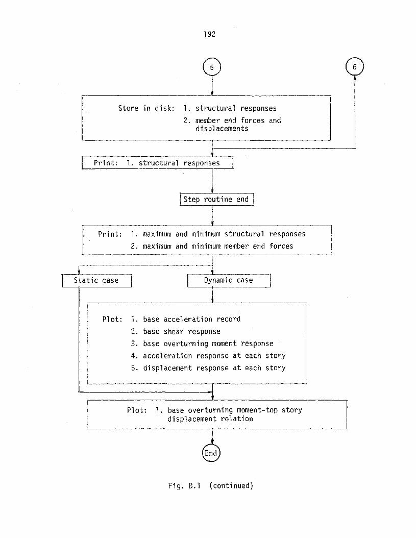
192

5 6

Store in disk: l. structural responses

2. member end forces anddisplacements

~

I Print: 1. structural responses I

IStep routi ne end I

Print: 1. maximum and minimum structural responses

2. maximum and minimum member end forces

I Static case I I Dynamic case I

Plot: 1. base acceleration record

2. base shear response3. base overturning moment response

4. acceleration response at each story

5. displacement response at each story

•Plot: l. base overturning moment-top story

displacement relation

~Fig. B.l (continued)

Documents

COMPUTED BEHAVIOR OF REINFORCED …shear walls behavior under these loads. Although there are many configurations and variations of shear wall systems in use, the analytical model