Computational Science and Engineering (International

Computational Science and Engineering(International Master’s Program)

Technische Universitat Munchen

Master’s Thesis

Comparison of Implementation Strategies forPDE Adjoint Problems

Rebecca Elisabeth Brydon

Computational Science and Engineering(International Master’s Program)

Technische Universitat Munchen

Master’s Thesis

Comparison of Implementation Strategies for PDEAdjoint Problems

Author: Rebecca Elisabeth Brydon1st examiner: Univ.-Prof. Dr. Michael Bader (TUM)Assistant advisor: Lukas Krenz (TUM)Assistant advisor: Dr. Anne Reinarz (Durham University)Submission Date: June 15th, 2021

I hereby declare that this thesis is entirely the result of my own work except where other-wise indicated. I have only used the resources given in the list of references.

June 15th, 2021 Rebecca Elisabeth Brydon

Acknowledgments

I would like to thank my supervisors Dr. Anne Reinarz (Durham University) and LukasKrenz (Technical University Munich) for their support and supervision! I would also liketo thanks Prof. Micheal Bader of the to the Scientific Computing department for giving

me the opportunity to write my master thesis at the research chair.A second big thank you to Anne Reinarz, for helping me apply as a visiting student at

Durham University. Many thanks to the Computer Science Department at the Universityof Durham for giving me the opportunity to visit Durham University.

vii

Irrtumer haben ihren Wert; jedoch nur hier und da. Nicht jeder, der nach Indien fahrt, entdecktAmerika.

-Erich Kstner

viii

Abstract

Common problems in seismology are: detecting the depth of soil layers, approximatingthe material parameters or determining the origin of an earthquake. These parameters canbe determined by solving an Optimal Control Problem. In this thesis, we consider AdjointProblems and how they can be used for parameter optimizations. As a gradient basedoptimization routine would require the first derivative of the cost function with respect tothe optimization parameter [1

.

]. A cost function J computes the cost as the norm betweenthe measurements and a simulated solution which is dependent on the model parameters.As the cost function is a composite function and depends on the PDE parameters α andalso on the PDE solution, the gradient DJ/Dα can not be computed so easily [2

.

]. It is thesecond dependency makes things more complex, as in most cases there is no functionalrepresentation of the PDE solution which would be directly differentiated. A solution isto compute the derivative via the adjoint equation of the PDE [1

.

]. In this thesis two ap-proaches for computing the total derivative are compared. The first approach Differentiate-then-discretize derives the adjoint equation analytically and then is discretized using theDG method [1

.

]. The second ansatz, Discretize-then-Differentiate, uses Automatic Differenti-ation (AD) to differentiate an already discrete forward solver [1

.

]. We create two prototypeimplementations of both adjoint solver approaches in the Discontinous Galerkin solverTerraDG [3

.

]. For comparison, we also implement the hyperbolic model equations in FEn-iCS, an open-source finite element solver which provides a python interface [4

.

], [5

.

]. Thedolfin-adjoint package [6

.

] can then be used to automatically compute the gradient via theadjoint.

ix

Contents

Acknowledgements

.

vii

Abstract

.

ix

I. Introduction

.

1

1. Introduction

.

31.1. Inverse Problems in Wave propagation

.

. . . . . . . . . . . . . . . . . . . . . . 3

II. Theory: Adjoint equations in Optimal Control Problems

.

5

2. Hyperbolic wave problems

.

72.1. Test equations

.

. . . . . . . . . . . . . . . . . . . . . . . . . . . . . . . . . . . . 72.1.1. Advection equation

.

. . . . . . . . . . . . . . . . . . . . . . . . . . . . 72.1.2. Linear elastic wave equations

.

. . . . . . . . . . . . . . . . . . . . . . . 82.1.3. Benchmark problem: Layer-over-halfspace 1 (LOH1)

.

. . . . . . . . . 10

3. Adjoint equations in Optimal Control Problems

.

133.1. Optimal control problems

.

. . . . . . . . . . . . . . . . . . . . . . . . . . . . . 133.2. Deriving the Adjoint equation

.

. . . . . . . . . . . . . . . . . . . . . . . . . . . 143.2.1. Deriving the adjoint using the Lagrangian function

.

. . . . . . . . . . 153.2.2. Deriving the adjoint system using the product rule

.

. . . . . . . . . . 173.3. Gradient computation using the adjoint

.

. . . . . . . . . . . . . . . . . . . . . 193.3.1. Gradient formulation using the Lagrangian: Advection equation

.

. . 193.4. Adjoint system for time dependent PDEs

.

. . . . . . . . . . . . . . . . . . . . 22

III. Implementation

.

25

4. Implementation

.

274.1. FEniCS and Dolfin-Adjoint using Python

.

. . . . . . . . . . . . . . . . . . 274.1.1. Basic methods and data structures

.

. . . . . . . . . . . . . . . . . . . . 274.1.2. Weak formulation for the hyperbolic wave equation using DG-elements

.

28

xi

Contents

4.1.3. Computation of the gradient using Dolfin-Adjoint and parameteroptimization

.

. . . . . . . . . . . . . . . . . . . . . . . . . . . . . . . . . 304.2. TerraDG using Julia

.

. . . . . . . . . . . . . . . . . . . . . . . . . . . . . . . . . 334.2.1. Differentiate-first-then-discretize

.

. . . . . . . . . . . . . . . . . . . . . 334.2.2. Discretize-first-then-differentiate using AD

.

. . . . . . . . . . . . . . . 35

IV. Results

.

39

5. Tests

.

415.1. Convergence tests

.

. . . . . . . . . . . . . . . . . . . . . . . . . . . . . . . . . . 415.1.1. Test equation convergence rates

.

. . . . . . . . . . . . . . . . . . . . . 415.1.2. Gradient convergence rates

.

. . . . . . . . . . . . . . . . . . . . . . . . 435.1.3. Convergence test for the TerraDG adjoint solver

.

. . . . . . . . . . . . 435.2. Visualization

.

. . . . . . . . . . . . . . . . . . . . . . . . . . . . . . . . . . . . . 485.2.1. Plots of the approximated solutions

.

. . . . . . . . . . . . . . . . . . . 485.2.2. Graph visualization methods in FEniCS

.

. . . . . . . . . . . . . . . . 48

6. Numerical Results

.

516.1. Paremeter optimization results

.

. . . . . . . . . . . . . . . . . . . . . . . . . . 516.1.1. Optimization example 1: Initial disturbance origin of LOH1

.

. . . . . 51

V. Conclusion

.

55

7. Conclusion

.

57

Bibliography

.

59

xii

Part I.

Introduction

1

1. Introduction

1.1. Inverse Problems in Wave propagation

In science we often make some observations of a physical phenomena and record these asmeasurement data. An Inverse Problem (IP) arises, if we want to determine the parameterswhich caused the phenomena but can not be measured. In this thesis we consider AdjointProblems and how they can be used for parameter optimizations.

Common problems in seismology are: detecting the depth of soil layers, approximatingthe material parameters or determining the origin of an earthquake. These parameterscan be determined by solving an Optimal Control Problem. A very good introduction toOptimal Control Problems in Flow Optimization is given in [1

.

]. For example, assume theorigin (sx, sy) of an earthquake is to be determined. We have recorded some measurementsof the displacement or the stress. A gradient based optimization routine would require thefirst derivative of the cost function with respect to the optimization parameter [1

.

]. A costfunction J computes the cost as the norm between the measurements and a simulatedsolution which is dependent on the model parameters. As the cost function is a compositefunction and depends on the PDE parameters α and also on the PDE solution, the gradientDJ/Dα can not be computed so easily [2

.

]. It is the second dependency makes things morecomplex, as in most cases there is no functional representation of the PDE solution whichwould be directly differentiated. A solution is to compute the derivative via the adjointequation of the PDE [1

.

].In this thesis two approaches for computing the total derivative are compared. The first

approach Differentiate-then-discretize derives the adjoint equation analytically and then isdiscretized using the DG method [1

.

]. However, the derivation of the adjoint equation canquickly become quite complex and has to be derivation specifically for the considered PDE.This is why it is interesting to look at a second ansatz: Discretize-then-Differentiate. In thiscase we use Automatic Differentiation to differentiate an already discrete forward solver[1

.

]. The advantage is that the AD computation can be implemented generically for all PDEequation of a certain form. On the other hand the computational cost for computing thegradient with AD are however quite high. We create two prototype implementations ofboth adjoint solver approaches in the Discontinous Galerkin solver TerraDG [3

.

]. For com-parison, we also implement the hyperbolic model equations in FEniCS, an open-sourcefinite element solver which provides a python interface [4

.

], [5

.

]. The dolfin-adjoint package[6

.

] can then be used to automatically compute the gradient via the adjoint. For testing,a parameter optimization example is setup following the general structure of the dolfin-adjoint tutorials [7

.

].

3

Part II.

Theory: Adjoint equations in OptimalControl Problems

5


A general formulation of a hyperbolic partial differential equation (PDE) is given in [8

.

] as

∂φ

∂t+∇ · Fc(φ) = f, (2.1)

where φ is the state vector and Fc(φ) represents the physical flux. In the following we usethe general Discontinuous Galerkin (DG) formulation N (u, v) given [9

.

] for a convective-diffusive system. As the above PDE system is only convective, we adapt the general for-mulation by setting the viscous terms in N (u, v) to be zero. We also disregard the interiorpenalty term for simplicity. The reduced DG-formulation then is

N (u, v) =−∫

ΩF(φ)∇vdx−

∫Ωf · v dΩ (2.2)

+∑κ∈T

∫Γ\∂Ω

H(φ, n+) · v+ ds (2.3)

+

∫ΓH(φ, gD, n+) · v ds = 0.

As defined in [9

.

], the domain Ω with the boundary Γ = ∂Ω is discretized on a mesh T withthe elements κ where ∂κ is the boundary of an element and nk is the outward pointingnormal on a face. The numerical flux H is approximated using the local Lax-Friedrichsflux given in [9

.

] defined as

H(φ, n+) = φ · n+ +1

2λmax · [[φ]], (2.4)

where φ = 12(φ+ + φ−) is the average and [[φ]] = φ+ − φ− is the jump [9

.

].

2.1. Test equations

2.1.1. Advection equation

The simplest hyperbolic wave equation is the linear advection equation. We use the defi-nition for a constant flow given in [10

.

]

∂φ

∂t+ β · ∇φ = 0 in Ω× (0, T ) (2.5)

φ(t,x) = φ0(x− βt) in ∂Ω× (0, T )

φ(0,x) = φ0(x) in Ω at t = 0

7


where the flow velocity in two dimensions is assumed to be the vector β = [βx βy]T . In

one dimension the flow velocity becomes a scalar [8

.

]. The initial condition at t = 0 overthe domain Ω is given by a function φ0, depending only on x. The boundary conditionare defined using the exact solution, which can be computed according to [8

.

], as the initialsolution shifted by the flow velocity depending on the current time t. An example initialcondition in two dimensions is the mock one-dimensional setting φ0(x) = sin(2πx).

2.1.2. Linear elastic wave equations

As a more advanced example equation, we consider the linear elastic wave equation, as itis a common base model used in seismology [8

.

]. To better understand the physical forcesconsidered by the model, we look at the simple example given in [8

.

] of a two dimensionalbeam. If the beam is compressed at [x = 0, y], the force will cause a ”pressure” wave,often shorted to P-wave, to propagate along the x-axis with the wave speed cp. As theequation system couples the stress φ and the motion u, the P-wave will accelerate thewave motion. The model however only holds if the deformations inside a solid are small,as in this case stress and strain can be linearly related by Hook’s law [8

.

]. For compressionforces, the behaviour of the elastic wave in solids is analogous for acoustic waves in gasor liquids. However, on solids there is a second type of force: the shear force. If the solidis displaced in y-direction, the material will show small elastic deformations. As long asthe deformations are small enough, the bonds between the molecule of the solid will try torestore the original state. The resulting waves are called S-waves and move orthogonalityto the direction of wave motion with wave speed ss. The equation system is only linear, ifthe deformations are linearly proportionally to the restoring forces. If the material is overstretched to breaking point, the resulting behaviour would clearly no longer be linear.

The elasticity equation system is given in [11

.

] in second order form as

ρ∂2u

∂t2−∇σ = 0 in Ω× (0, T ) (2.6)

σ · n = T in Γ× (0, T )

u = u0(x) in Ω, t=0

which relates the displacement u, the stress σ and the acceleration ∂2u∂t2

. The material den-sity is given by ρ. As DG formulations are generally derived for first order PDE system, weconsider the first order derivations and equation definitions given in [8

.

]. The three dimen-sional elastic wave equation can be reduced to a two dimensional plane if the variationsin the third direction is zero. The five equations (2.7

.

), defined in [8

.

], can be used to model

8

2.1. Test equations

the motion of S-waves and P-waves in a two dimensional plane.

∂

∂t

σ11

σ22

σ12

uv

− ∂

∂x

(λ+ 2µ)u

λuµv

1ρσ

11

1ρσ

12

− ∂

∂y

λv

(λ+ 2µ)vµu

1ρσ

11

1ρσ

22

= 0. (2.7)

For some simpler setups, e.g. the planar wave problem given in [12

.

], it is still possible tofind an analytic solution which can be applied at the boundary. When computing a seismicsimulation, for example the simple LOH1 earthquake scenario, a physically motivatedboundary condition must be applied [8

.

]. We follow the boundary condition approachgiven in [8

.

], where the exterior ghost cells out side the domain are set based on the interiorcells in a physically meaning full way. This means for the ghost layer at the boundary wemust ether specify a motion, i.e. set the velocities u, v or specify a traction Tbnd by settingthe components of the stress in normal direction (outward pointing) according to

T = σ · ~n (2.8)Tout = 2 · Tbnd − Tinuout = uin

vout = vin.

For the left and right boundary this means setting σ11 and σ12, for the top/bottom bound-ary T = [σ22 σ12]T . The stress perpendicular to the normal vector, σ11 for n = (0, 1) andσ22 for n = (1, 0), can not be controlled. If T = 0, then the boundary is called a traction freeboundary and the velocities are simply copied from inside the domain [8

.

].

Planar wave problem in one dimension

The two dimensional system can be reduced to a single dimension as shown in [8

.

], by set-ting setting the displacements in y-direction to zero. The two decoupled one-dimensionalsystems, model the P-waves in x-direction and S-waves in y-direction separately [8

.

]. Asan test case, use the system derived for the displacements in y-direction in [8

.

] as

∂σ12

∂t− µ∂v

∂x= 0 (2.9)

∂v

∂t− 1

ρ

∂σ12

∂x= 0,

with the wave speed cs and the analytical solution given in [13

.

] as

v(x, t) =1

2(sin(2π(x+ cst)) + sin(2π(x− cst))) (2.10)

u(x, t) =1

2(sin(2π(x+ cst)) + sin(2π(x− cst))).

9


Planar wave problem in two dimension

We use the three dimensional planar wave problem given in [12

.

] and reduce it to a twodimensional domain Ω = [0, 1]2. The given analytical definition of the displacement inthree dimension, is dependent on the three unit vectors p, dp and dp. By setting the wavepropagation direction p =

[1 0 0

]T to move in x-direction instead of z, the componentsin the third dimension fall away. The P-Wave is set the same way, as it must run parallelwith dp = p =

[1 0 0

]T [12

.

]. The S-Wave propagates tangentially and therefore stays

ds =[0 1 0

]T . Inserting p,dp and ds into the analytic displacement definition, gives

δ1 = cos(k(x− cpt)) δ2 = cos(k(x− cst)) (2.11)

ans we can derive the analytical solutions for the velocities by differentiating δ w.r.t. to tgiving

u = cpksin(k(x− cpt)) v = csksin(k(x− cst)). (2.12)

For this test example, we use the analytical solutions to periodic boundary conditions.However, as we use the elastic wave equation in the stress-velocity formulation, we mustalso compute an analytic definition for the strain. For this we can use the relation given in[8

.

]:

ε =1

2[∇~δ + (∇~δ)T ] =

−k sin(k(x− cpt)) −0.5k sin(k(x− cst)) 0−0.5k sin(k(x− cst)) 0 0

0 0 0

. (2.13)

As the only non-zero strain components are ε11 and ε12, the equation system [(22.11),[8

.

]]can be simplified to compute the x and y stress components as

σ11 = ε11(λ+ 2µ) (2.14)

σ22 = ε11λ

σ12 = 2ε12µ.

2.1.3. Benchmark problem: Layer-over-halfspace 1 (LOH1)

A common model for simulating a basic earthquake scenario is the Layer-over-Halfspace1 (LOH1) setup. The three dimensional setup given by [14

.

] is used in the following butreduced to two dimensions along the y-z-plane. The domain dimensions are used forthe FEniCS model as specified in the setup. For TerraDG the domain Ω is extended inz-direction to be come square, as non square domains are not jet supported. Figure ??shows how the domain is divided into two sub-domains: a shallow layer on top of a largehalf-space. In the setup given in [14

.

] an initial disruption is given by a point source whichis located at twice the layer depth below the surface (top edge). An alternative way to

10

2.1. Test equations

Figure 2.1.: The LOH1 setup following: The domain is subdivided into a layer region, witha 1km depth and a large half-space below [14

.

]. The origin point of the sourceis located 2km below the top surface .

introduce an initial disruption without a point source is to set an initial stress in the twonormal directions σ11 and σ11 in form of a tow dimensional Gaussian curve which has thecenter points (sx, sy). As the initial condition must satisfy the boundary condition givenin (2.9

.

), the Gaussian curve (2.15

.

) is clamped to zero at the width Lx and height Ly of thedomain.

φ110 = exp(−0.01(x−sx)−0.01(y−sy)2)(Lx − x)x(Ly − y)y (2.15)

φ220 = exp(−0.01(x−sx)−0.01(y−sy)2)(Lx − x)x(Ly − y)y

The remaining components φ12, u and v are initialized with zero. As the domain dimen-sions and parameter settings are given in SI units, the problem length is scaled to [km]with the scaling constant SL = 10e3. The flow speeds cs and cp are scaled analogously to[km/s].

11

3. Adjoint equations in Optimal ControlProblems

3.1. Optimal control problems

A common problem in many application fields of PDE models, is determining equationparameters based on a chosen cost function J , also called objective functional [1

.

]. In thefollowing section, we follow the general definitions given in [1

.

] of an optimal control prob-lem for a PDE F with state variables φ and the parameter α is given in [1

.

] as

minimizeα

J(α, φ(α), t)

subject to F (φ(x, α), α, t) ≡ 0, x ∈ Ω, t ∈ (0, T ).

The goal is to determine an optimal parameter value αopt which minimize the cost functionJ , under the constraint that αopt and corresponding solution vector φopt satisfy the PDEequation. For the optimization of the cost functional, a gradient based optimization routinecan be used. However, these requires the gradient of the optimized function to determinethe new search direction of the next step. A short summary of the symbols used in thischapter is given in Table (3.1

.

).

Cost/objective function

A general formulation of a cost function which computes the cost over the complete timeand space domain is given in [1

.

] as

JT (φ, α) =γ1

2

∫ T

0

∫Ω

(φ− Φ)2dΩdt (3.1)

+γ2

2

∫Ω

(φ |t=T −Φ |t=T )2dΩ + γs.

We follow the explanation in [1

.

], of the three terms of the cost functional to understandthe motivation for choosing the given form. The first integral computes the difference be-tween the solution φ and a measured solution Φ over the complete time and space domain.The second integral term is in principle already included in the first, as the time integralincludes the final time T , it however improves the optimization results. The penalty term

13


γs = σ2

∑Kk=1 α

2k prevents the optimal control parameter value to become too large. An

often used simplification of this cost function is obtained by setting γ1 = 0, giving

JC(φ, α) =γ2

2

∫Ω

(φ |t=T −Φ |t=T )2dΩ + γs. (3.2)

The time integral falls away and the cost is only computed using φ at the final time step.Equation (6.1

.

) can also called a controllability functional [1

.

]. In theory, one can compute thecost function at every node xi,j for i, j = [1, . . . , N ] of the discretized mesh. However, inpractice it is simply infeasible to take so many measurements. We remind ourselves ofthe LOH1 setup, given in [14

.

], where the displacement caused by an initial disruption aremeasured only at a few sensor points and not over the entire domain. We define the costfunction then as

JS(φ, α) =1

2

M∑k=0

S∑i,j=0

(φ(xi,j , t)− Φ(xi, t)2dt+

S∑i,j=0

(φ(xi,j , T )− Φ(xi, T )2dt, (3.3)

where S is the number of sensor points and M the number of time steps.

3.2. Deriving the Adjoint equation

There are different approaches for deriving the first derivative i.e. the total derivative DJDα

of the cost function J with respect to the equation parameters. The two main approachescan be divided into two categories, depending on the order in which the approach dis-cretizes and differentiates the equations. Figure (3.1

.

) visualizes the two different compu-tation paths, which in the limit should converge to wards the same solution.

Figure 3.1.: Comparison visualization of the two approaches: first differentiate then dis-cretize or vice versa.

Differentiate-first-then-discretize: The total derivative can then be computed by first settingup the Lagrangian for the optimal control problem and then differentiating with respect to

14


F (φ) PDE dependent on the state vector φΛ Adjoint variableJ cost / objection functionalα general symbol for equation parametersΩ domain for x, y ∈ [0, 1]2

Γ boundary of domaint time, t0 = 0 start time and T = 1 end time

Table 3.1.: Symbols used for the definition of the optimal control problem and the deriva-tion of the adjoint system.

the Lagrangian multipliers to obtain the adjoint equation. The cost function and the PDEwith the corresponding adjoint equation is then be discretized.

Discretize-first-then-differentiate: The PDE equation system and the cost function are bothdiscretized first and implemented in code. The differentiation to compute the adjoint equa-tion is done using automatic differentiation (AD).

3.2.1. Deriving the adjoint using the Lagrangian function

In the following section, we derive the adjoint equation closely following the examplederivation for the heat equation given in [1

.

]. The Lagrangian function of an optimal con-trol problem consists of four parts: the cost function, the PDE rearranged equal to zero,the boundary and initial conditions also rearranged to zero. As an initial example, theLagrangian function with the multipliers Λ, τ and η is setup for the advection equation:

∂φ

∂t+ β∇ · φ = 0 in (0, T )× Ω, (3.4)

φ = g on (0, T )× Γ, (3.5)φ = φ0 in at t = 0. (3.6)

The Lagrangian function for the PDE definition then is:

L(φ, α,Λ, τ, η) = J(φ, α) −∫ T

0

∫Ω

Λ ·(∂φ∂t

+ β∇φ)dΩdt︸︷︷︸

Integral over the PDE must be zero

(3.7)

−∫ T

0

∫Γτ ·(φ− g

)dΓdt︸︷︷︸

Integral over BC must be zero

(3.8)

−∫

Ωη ·(φ |t=0 −φ0

)dΩ︸︷︷︸

Integral over IC must be zero

. (3.9)

15


Setting the derivatives w.r.t to the Lagrangian multipliers Λ, τ and η equal to zero shouldrecover the original PDE problem [1

.

]. We can test this for the state equation by computing

dL

dΛ= lim

ε→0

1

ε

(L(φ, β,Λ + εΛ, τ, η)− L(φ, β,Λ, τ, η)

)(3.10)

= limε→0

1

ε

(−∫ T

0

∫ΩεΛ ·

(∂φ∂t

+ β∇φ)dΩdt

). (3.11)

The variation ε cancels out and as we can choose Λ arbitrarily, the original PDE is recov-ered. To derive the adjoint equation we derivative of L w.r.t. the state variable and equalto zero:

∂L

∂φ=γ1

∫ T

0

∫Ω

(φ− Φ)φdΩdt+ γ2

∫Ω

(φ |t=T −Φ |t=T )φdΩ (3.12)

−∫ T

0

∫Ω

Λ(∂φ

∂t+ β∇φ)dΩdt−

∫ T

0

∫Γτ(φ− gD)dΓdt (3.13)

−∫

Ωη(φ |t=0)dΩ (3.14)

Applying integration by parts derives the adjoint equation. We obtain

∂L

∂φ=

∫ T

0

∫Ωφ(∂Λ

∂t+ β∇Λ) + γ1(φ− Φ)

)dΩdt (3.15)

−∫

Ω(Λ |t=T −γ2(φ |t=T −Φ |t=T ))φ |t=T dΩ (3.16)

−∫ T

0

∫Γτ(φ− gD)dΓdt+

∫Ωφ |t=0 (Λ |t=0 −η)dΩ (3.17)

−∫ T

0

∫Ωφ · ΛdΓdt (3.18)

The two equations which result from the Lagrangian multipliers τ and η are not reallyrelevant for the adjoint problem. Adjoint system given then is

−∂Λ

∂t− β∇Λ = γ1(φ− Φ) (T, 0)× Ω (3.19a)

Λ = 0 (T, 0)× Γ (3.19b)Λ = γ2(φ |t=T −Φ |t=T ) Ω at t = T. (3.19c)

is also an advection equation but with the computation time reversed. The source is gen-erated by the first integral term of the time dependent time cost function J in (3.1

.

). The

16


initial condition of the adjoint equation is generated by the second integral of the timedependent time cost function J in (3.1

.

).Setting the derivative of L w.r.t. to the optimization parameter equal to zero, we could

derive the so called optimality conditions. The ”one-shot method” combines these with thePDE and the adjoint equation to form the optimality system. According to [1

.

], advantageof the one-shot method, is that if the combined system is solvable, the solution is alsodirectly the desired optimum. However, as the number of unknowns in the combinedsystem is more than double that of the PDE system, solving the optimality system directlyis often not possible. Even iterative methods may not converge.

A perhaps more intuitive way to compute the derivative is shown in [1

.

] by go via thesensitivity equation. The sensitivity equation can be obtained by differentiating the PDEequation with w.r.t. to the optimization parameter β using the chain rule:

∂

∂β

(∂φ∂t

+ β(∇ · φ) = 0)

= 0. (3.20)

To simplify the partial derivative notation, the partial w.r.t. to the parameter is denoted as:φβ = ∂φ

∂β . The sensitivity equation for the advection is:

∂φβ∂t

+ β∇ · φβ = −∇ · φ (0, T )× Ω (3.21a)

φβ = 0 (0, T )× Γ

φ = 0 in Ω at t = 0

For a PDE with K parameters, this would result in K sensitivity equations. To computethe total derivative for each parameter, K equations must be solved. Already for a smallnumber of 3 − 5 parameters this would be costly. The reason for making a larger effort infurther deriving the adjoint equation (3.19a

.

), is that it must only be set up once and can beused to compute the derivative for multiple parameters. Instead of solving K equations,only a single equation is solved and then used to compute the K different derivatives.

3.2.2. Deriving the adjoint system using the product rule

A more general formulation of the adjoint and gradient derivation is given in [1

.

] and [2

.

].In this section we follow this general approach, to obtain a matrix-vector formulation ofthe gradient. The general formulation of the cost function

J(α, φ(α))

contains a direct dependency on the parameter α and the state variable φ but also has anindirect dependency on α via φ. We follow the derivation steps in [1

.

] and compute thegradient of the cost functional by applying the chain rule to obtain the total derivative:

DJ

Dα=∂J

∂φ

dφ

dα+∂J

∂α(3.22)

17


The explicit formulation of the cost functional J is known, whether this is in exact ana-lytical form or as a discrete function. The terms ∂J

∂φ and ∂J∂α can therefore be computed

normally using the standard derivation rules. On the other side, the Jacobian matrix dφdα of

the state variable φw.r.t. the parameter α is not trivial to compute. In most cases there is noexplicit formulation of the PDE given, which we could directly differentiate. Additionally,the derivative matrix is fully dense and therefore expensive to compute and store [2

.

]. Inorder to avoid the direct computation of this term, the adjoint equation(∂F

∂φ

)TΛ =

(∂J∂φ

)T, (3.23)

given in [1

.

] can be substituted into (3.22

.

) giving:

DJ

Dα= ΛT

∂F

∂φ

dφ

dα+∂J

∂α. (3.24)

The adjoint equation (3.23

.

) was derived in [1

.

] by setting up the Lagrangian function, asshow in section (3.2.1

.

), but for the more general formulation. Finally, the term ∂F∂φ

dφdα can

be replaced by inserting the sensitivity equation. We can derived it by applying the chainrule to the PDE system w.r.t. state variables as

d

dαF (φ, α) = 0 (3.25)

∂F

∂φ

dφ

dα+∂F

∂α= 0

∂F

∂φ

dφ

dα= −∂F

∂α.

Inserting (3.25

.

) into (3.24

.

) gives the equation

DJ

Dα= −ΛT

∂F

∂α+∂J

∂α(3.26)

for computing the derivative of the functional w.r.t. the parameters. Slightly differentderivation steps are shown in [2

.

], which derive the adjoint equation by going via the sen-sitivity equation. If we inverting the last line of the sensitivity equation, we obtain

dφ

dα=(∂F∂φ

)−1(− ∂F

∂α

). (3.27)

This equation can then be used to replace the problematic derivative dφdα in (3.22

.

) giving

DJ

Dα=∂J

∂φ

(∂F∂φ

)−1(− ∂F

∂α

)+∂J

∂α. (3.28)

18

3.3. Gradient computation using the adjoint

By taking the Hermitian transpose of the system

DJ

Dα

∗=∂J

∂φ

∗ (∂F∂φ

)−∗(− ∂F

∂α

)∗︸︷︷︸

=Λ

+∂J

∂α

∗. (3.29)

one can obtain the same adjoint equation and total derivative as in Equation (3.26

.

). As wecan assume that the derivative values are real valued, we replace the Hermitian A∗ withthe transpose AT when using the formulations given in the following sections.


3.3.1. Gradient formulation using the Lagrangian: Advection equation

Now that the adjoint equation was obtained via the Lagrangian, we can compute the totalderivative by differentiating the cost function with respect to the optimization parameters,in our example this is the flow velocity. By deriving J w.r.t. β we obtain:

DJ

Dβ=

∫ T

0

∫Ω

(φ− Φ)φβdΩdt+

∫Ω

(φ |t=T −Φ |t=T

)φβ |t=T dΩ (3.30)

=

∫ T

0

∫Ω

(− ∂Λ

∂t− β∇ · Λ

)φβdΩdt+

∫Ω

(Λ)φβ |t=T dΩ (3.31)

Now we can use the adjoint equation to replace the term φ−Φ and the terminal conditionof the adjoint equation to replace the term φ |t=T −Φ |t=T . Integrating the resulting systemby parts over time and space gives:

DJ

Dβ=

∫Ω

∫ T

0Λ∂φβ∂t

dtdΩ−∫

Ω(Λφβ) |t=Tt=0 dΩ (3.32)

+

∫ T

0

∫Ω

Λ∇ · φβdΩdt−∫ T

0(φβ∇ · Λ · ~n) |Γ dt (3.33)

+

∫Ω

Λφβ |t=T dΩ (3.34)

By re-arranging the equation system

DJ

Dβ=

∫Ω

∫ T

0Λ(∂φβ∂t

+∇ · φβ)dtdΩ−

∫Ω

(Λφβ) |t=Tt=0 dΩ (3.35)

−∫ T

0(φβ∇ · Λ · ~n) |Γ dt (3.36)

+

∫Ω

Λφβ |t=T dΩ, (3.37)

19


we can see how the conditions from (3.21a

.

) and (3.19a

.

) cancel out all single integral termsor are equal to zero. The equation with φβ can be substituted with the right hand side ofthe sensitivity equation. The total derivative can therefore be expresses as:

DJ

Dβ=

∫Ω

∫ T

0Λ · φβ dtdΩ (3.38)

Gradient formulation using the Lagrangian: Elastic wave equation

For the second test equation, the elastic wave equation, we have to do the same stepsfor deriving the adjoint equation and total derivative formulation. We again follow thederivation steps given in [1

.

]. In the following we only make a first attempt at the derivationof the adjoint equation. We follow the first steps to show that we expect the elastic waveadjoint to be self-adjoint [11

.

].The general optimal control problem is:

minimizeC

J(u,C, a, b, c)

subject to F (u,C, a, b, c) = ρ∂2u

∂t2−∇ · σ = 0 in Ω× (0, T )

σ · n = T in Γ× (0, T )

u = u0(x) in Ω, t=0

Setting up the Lagrangian the same way as shown previously, we obtain

L(u,C, a, b, d) = J(u,C)−∫ T

0

∫Ωa(ρ∂2u

∂t2−∇σ

)dΩdt︸︷︷︸

F (u,C,a)

(3.39)

−∫ 1

0

∫Ωb · (σ · n− T )dΓdt︸︷︷︸BC(u,C,b)

−∫

Ωc · (u |t=0 −u0(x)) dΩ︸︷︷︸

IC(u,C,c)

Deriving w.r.t. the Lagrangian multipliers a

∂L

∂a= lim

ε→0

1

ε

(− F (u,C, a+ εa)− (−F (u,C, a))

)(3.40)

= limε→0

1

ε

(∫ T

0

∫Ωεa(ρ

∂2u

∂t2−∇σ) dΩdt

)=

∫ T

0

∫Ω

(ρ∂2u

∂t2−∇σ) dΩdt

20


will make 1ε and ε cancel out and we obtain the original PDE system again, as we can ar-

bitrarily chose the variation. This can be done the same way for the other two multipliers.To obtain the adjoint equation system, we derive w.r.t. the state variable u.

∂L

∂u= lim

ε→0

1

ε

(L(u+ εu)− L(u)

)(3.41)

= limε→0

1

ε

(J(u+ εu)− J(u)

− F (u+ εu) + F (u)

−BC(u+ εu) +BC(u)

− IC(u+ εu)) + IC(u))

Two relations given in [11

.

] between the material parameter matrix C, the stress σ and thedisplacement u are used to rearrange the equations.

σ + εσ = C : E[u+ εu] = C : E[u] + C : E[εu] (3.42)

Following [11

.

], the divergence of the stress∇σ can be rewritten as:

∇ · σ + ε∇ · σ = ∇C : ∇(u+ εu) = ∇C : ∇u+∇C : ∇εu (3.43)

For the F term the derivation w.r.t. the state variable can be determined as:

= limε→0

1

ε

∫ T

0

∫Ωa(− ρ∂

2u+ εu

∂t2+∇(σ + εσ) + ρ

∂2u

∂t2−∇σ

)dΩdt (3.44)

=

∫ T

0

∫Ωa(− ρ∂

2u

∂t2+∇σ

)dΩdt (3.45)

Integrating by parts twice over time to move derivative onto Lagrangian multiplier givesus: ∫ T

0−ρa∂

2u

∂t2dt =

∫ T

0−ρu∂

2a

∂t2dt+

[ρu∂2a

∂t2

]T0

+[ρa∂u

∂t

]T0

(3.46)

Then we integrate by parts over space once and obtain∫Ω∇σdt =

∫Ω

(∇C) : (∇u)dt = −∫

Ω(∇ · C) : (∇a) · udΩ (3.47)

+

∫Γa(∇ · C) : (u)dΓ (3.48)

If we define (∇ ·C) : (∇a) = ∇ · σa, we can see the original elastic wave equation but nowwith the adjoint variable a as the unknown:

=

∫ T

0

∫Ωu(− ρ∂

2a

∂t2−∇ · σa

)dtdΩ (3.49)

+[ρu∂2a

∂t2

]T0

+[ρa∂u

∂t

]T0

+

∫Γa(∇ · C) : (u)dΓ (3.50)

21


We know from [11

.

], that the elastic wave equation should be self-adjoint, meaning that theadjoint equation is again an elastic wave equation. We can see this also in our derivationattempt for the adjoint equation in (3.50

.

). The remaining steps would include applying thederivation w.r.t. to the state variable φ to the boundary and initial condition parts of theLagrangian.

3.4. Adjoint system for time dependent PDEs

The above derivations both did not show directly the time dependency of the adjoint equa-tion. In this section we closely follow the steps in [15

.

] for computing the gradient usingthe adjoint solutions over the complete time. For a time dependent system the adjointequation is actually a system of equations

[∂F∂φ

]T︸︷︷︸

(n2·m)×(n2·m)

~Λ︸︷︷︸(m·n2)×1

=( ~∂J∂φ

)T︸︷︷︸(1×m·n2)

(3.51)

with a row per time level of the forward problem. The dimensions of the partial deriva-tives depend on the dimensions of the given optimization problem. The example consid-ered in [15

.

], computes the adjoint equation for the one dimensional advection equationusing Finite Differences to solve the PDE equation. The main steps in [15

.

] are howeververy general and can easily be used for our general example of a two dimensional PDEF = 0 with the state vector φ which has v variables. The domain is discretized on a(n × n) grid, with the indexes i, j = (1,1),(2,1), . . . , (n,n). The time is discretized withk = 0, . . . ,m time steps. All time levels of the system variable φ are stored in the vector~φ = [φ1

11, φ121, . . . , φ

1n1, . . . , φ

mnn]T of size (m · n2 × 1). The right hand side of the equation

system is given by the derivative of the cost function with respect to the state variable. Asthe cost function J is a single value per variable v, the derivative ∂J

∂α is also a scalar. Thepartial derivative ∂J

∂φ is a vector of size (1 ×m · n2). The adjoint vector, the unknowns, isΛ = [Λ0

11, . . . ,Λ01n, . . . ,Λ

m−1,Λm]T of the size (m ·n2× 1). To remind ourselves, the adjointequation is solved after having computed the forward solution φ.

Computing the derivative matrix ∂F∂φ

We start by looking at setting up the system matrix of the adjoint equation (3.51

.

). If thecomplete matrix ∂F

∂φ for all time levels would be set up, it would be a (mB × mB) blockmatrix with blocks of size (n2 × n2) which are the partial derivatives in space of a singletime step. As shown in the example given in [15

.

], only the diagonal and sub-diagonalscontain non-zero matrix blocks as shown in ( 3.52

.

). In the matrix the rows represent thetime levels. The PDE equation F k at time step k is only dependent on solutions φl where

22

3.4. Adjoint system for time dependent PDEs

l ≤ k. If the derivative of F k w.r.t. to a solution vector φl at a time step l > k is made, thiswould clearly be zero. This means all derivatives above the diagonal are zero.

∂F

∂φ=

∂F 0

∂φ00 . . . 0

∂F 1

∂φ0∂F 1

∂φ1. . . 0

......

∂Fm

∂φ0∂Fm

∂φ1. . . ∂Fm

∂φm

(3.52)

In practice, setting up the large time dependent system is not necessary, as the matrix ismostly sparse depending on the chosen time stepping. We use the same time steppingmethod as in [15

.

], the Euler method method

F k =1

∆t

(φk − φk−1

)+ ∆φ = 0 (3.53)

but using the backward definition [16

.

]. Each time level k depends on the previous level(k − 1). The resulting derivative matrix would only have non-zero block entries on thediagonal and the sub-diagonal as shown in (3.57

.

).Each entry of the full time matrix is in turn a derivative matrix but in x and y-direction

[15

.

]. In each matrix row contains two non-zero partial derivative matrices at the time stepk and (k − 1). The partial derivatives of F at the time step k can easily be determined byderiving the Euler equation w.r.t. φk, as a diagonal matrix (3.54

.

) with the time step 1∆t on

the diagonal.

U1 =∂F kij

∂φkij=

1

∆t. . .

1∆t

(3.54)

The sub-matrix (3.55

.

) of the partial w.r.t. to the state vector φk at time step (k − 1) is alsoa sparse matrix, with non-zero entries depending on the chosen discretization scheme inspace [15

.

]. The matrix is given in the transposed form as:

U2 =( ∂F kij

∂φk−1ij

)T=

∂Fki,1

∂uk−1i,1

∂Fki,2

∂uk−1i,1

0 0 . . . 0

0∂Fki,2

∂uk−1i,2

∂Fki,3

∂uk−1i,2

0 . . . 0

0 0 0. . . ∂Fki,n

∂uk−1i,n−1

∂Fki,n

∂uk−1i,n

(3.55)

As the equation system is two dimensional, every matrix entry is the y-derivative at j,for every point i in x-direction. The structure of theses sub-sub-derivative matrices staysthe same. The matrix example above is given disregarding boundary conditions. For a

23


first order Finite Volume (FV) stencil, approximating the flux with the local Lax-FriedrichsMethod, each row contains at most five non-zero entries. Matrix U2 in (3.56

.

) gives realvalued example for a small 9 × 9 grid when applying a FV discretization on the two di-mensional advection equation. Here we can also see how the boundary conditions changesthe sparsity pattern of the derivative matrix.

U2 = −

1.5 0.0 0.75 0.0 0.0 0.0 0.75 0.0 0.00.75 1.5 0.0 0.0 0.0 0.0 0.0 0.75 0.00.0 0.75 1.5 0.0 0.0 0.0 0.0 0.0 0.750.75 0.0 0.0 1.5 0.0 0.75 0.0 0.0 0.00.0 0.75 0.0 0.75 1.5 0.0 0.0 0.0 0.00.0 0.0 0.75 0.0 0.75 1.5 0.0 0.0 0.00.0 0.0 0.0 0.75 0.0 0.0 1.5 0.0 0.750.0 0.0 0.0 0.0 0.75 0.0 0.75 1.5 0.00.0 0.0 0.0 0.0 0.0 0.75 0.0 0.75 1.5

(3.56)

Iterative scheme for the adjoint computation

For the analytical adjoint of the advection equation, it was shown that the time and advec-tion direction is reversed [2

.

].U1

1 U22 0 0 0

0 U21 U3

2 0 0. . . . . .

0 0 0 Um−11 Um2

0 0 0 0 Um1

·

Λ0

Λ1

...Λm−1

Λm

=

∂J∂φ0∂J∂φ1

...∂J

∂φm−1

∂J∂φm

(3.57)

We now can see the same: Starting with a terminal condition the end time T with Λm,the equation system (3.57

.

) is solved using back substitution for the initial solution Λ0. Fora PDE, for which the right hand side is independent of time, each time step will havethe same derivative. This means the time dependent system of equations (3.57

.

) simplifiesfurther, as Uk1 = Uk+1

1 and Uk2 = Uk−12 . The iterative scheme given in [15

.

] then reads as:

1. Start with U1Λm = ∂J∂φm

2. For k = m− 1, . . . , 1

U1λk =

( ∂J∂φk− λk+1U2

)(3.58)

24

Part III.

Implementation

25

4. Implementation


FEniCS is an open-source finite-element solver which translates a weak form written usinga python interface in UFL (Unified Form Language), into C++ Finite Element code [4

.

], [5

.

],[17

.

], [18

.

], [19

.

], [20

.

]. The major advantage of this is that the UFL problem formulationis very similar to the mathematical formulation. The package dolfin-adjoint overloadscertain FEniCS methods, to allow the computation of the gradient using the adjoint. Weuse FEniCS and dolfin-adjoint in the next section to implement the forward models of thetest equations and setup the optimal control problems.

4.1.1. Basic methods and data structures

We shortly go over the basic methods in FEniCS , as explained in the online tutorial book[21

.

]. In FEniCS every function is generated over a function space, which is generatedfrom the given domain mesh. The basic function space is generated by using the methodFunctionSpace. If every unknown in the function space is to be a vector, then one hasto set up a VectorFunctionSpace with the given vector dimension dim=N. The type ofbasis element is set by the parameter family, e.g. for standard continuous Lagrangianbasis functions the keyword CG is passed. For Discontinuous Galerkin elements the key-word DG is together with the element degree. The function Measure returns an operatorwhich computes the integral over a certain domain in the mesh. The integral over thedomain area is given by dx, while dS gives the integral over the inner facets and ds theintegral over the boundary facets.The method FacetNormal returns the outward point-ing face normal of the given mesh. Examples for these basic methods can be seen in thecode extract (4.1

.

). The FEniCS Expression class allows the user to define an C++ expres-sion which then is JIT (just-in-time) compiled, avoiding the overhead when making callsto a python defined function from the auto-generated C++ code [21

.

]. An example is givenfor the Lame parameter definition in code listing (4.7

.

). FEniCS also provides a simple-to-use interface for imposing strong Dirichlet and von-Neumann boundary conditions. Themethod DirichletBC(V, gD, on boundary) takes the function space, an expressiongD which gives the values at the boundary and a user defined function on function thatreturns a Boolean value if the mesh point x is on the boundary or not [21

.

]. A very sim-ple example is on boundary = lambda x : near(x[0], 0, tol), which only re-turns true if the point x is on the left boundary. When the solve function is called, theboundary object bcs is passed to be applied to the system matrices.

27

4. Implementation

1 V_dg = FunctionSpace(unit_mesh, 'DG', dg_order)2 V_vec_dg = VectorFunctionSpace(unit_mesh, 'DG', dg_order, dim=5)3

4 u, v = TrialFunction(V), TestFunction(V)5

6 dx = Measure('dx', domain=unit_mesh) # domain area7 dS = Measure('dS', domain=unit_mesh) # interior facet8 ds = Measure('ds', domain=unit_mesh) # boundary facets9

10 n = FacetNormal(unit_mesh) # get the normal vector

Source Code 4.1.: For a basic FEniCS setup a function space using a specified FE-elementtype is defined. The corresponding trial and test functions can easily beobtained from V. The measure objects dx, dS, ds compute the integralover a certain subdomain. The face normal ~n is the outward pointingnormal vector on the cell facet.

4.1.2. Weak formulation for the hyperbolic wave equation using DG-elements

In FEniCS the general variational formulation is

a(u, v) = L(v), (4.1)

where the left hand side a is dependent on both the u, the unknown state variable andthe test function v [21

.

]. All known terms are collected in the right hand side L(v). Anequivalent formulation is given by

F (u, v) = 0, (4.2)

if the sides are not split. The DG formulation defined in (2.2

.

) is generated with the methodL operator as shown in the code extract (4.2

.

). The main difference when using Discontin-uous Galerkin FE-elements is that the boundary conditions must be imposed weakly in thevariational formulation as defined in equation (2.2

.

). Translated into ufl code, source codeextract (4.2

.

) shows a general method for generating the weak formulation. As shown in[22

.

], the facet normal must be restricted when integrating over the interior facets. This canbe done using the restriction operator as shown in [23

.

], which selects ether the right ’+’or the left ’-’ side of the facet. The physical flux and the maximum velocity, i.e. the max-imum eigenvalue are equation specific. For the advection equation the flux passed wouldsimply be flux = beta * phi old as shown in [24

.

] and for the elastic wave equationthe flux definition is given in 4.5

.

. The dimensions of the flux must match the dimensionsand number of variables of the function space V, e.g. for the elastic wave equation theflux.ufl shape is (5,2). The general structure of a forward solve method using anexplicit Euler time discretization is shown in (4.3

.

). To add a higher order time stepping,we follow the example given in [25

.

], which shows how to implement the stabilized third

28


1 def L_operator(phi_old, flux, maxvel, gD, v, f, n):2 L = dot(grad(v), flux)*dx + dot(f, v)*dx3 flux_dS = dot(avg(flux), n('+')) + 0.5*maxvel('+')*jump(phi_old)4 flux_ds = 0.5*(dot((flux + gD*beta), n) + maxvel*(phi_old - gD))5 L -= inner(flux_dS, jump(v)) * dS6 L -= inner(flux_ds, v) * ds7 return L

Source Code 4.2.: UFL implementation of the variational formulation for the hyperbolicsystem F as defined under (2.1

.

). The face normal in the interior integralflux dS must be restricted as shown in [22

.

]. The boundary is weaklyimposed by using the boundary function gD to define flux at the bound-ary.

1 def forward(...):2 ... # Basic setup of Function Space V ect.3 u1 = Function(V, name='u1')4 u1 = project(ic, V) # project IC5 # variational formulation and time discretization6 F = - inner(dt * (u - u1), v) * dx # Euler time stepping7 F += L_operator(beta, u, gD, v, f, n)8 a, L = lhs(F), rhs(F)9

10 u_new = Function(V) # storage for computed time step n + 111 steps = int(t_end / dt) # set up time stepping12 t = dt13 gD.t = dt14

15 for n in range(1, steps):16 solve(a == L, u_new) # Alternatively: solve(F == 0, u_new)17 u1.assign(u_new) # update the variable18 t += delta_t19 gD.t = t # update boundary expression20

21 return u1, t

Source Code 4.3.: FEniCS implementation of the advection equation using DG elementsand Euler time stepping.

order strong-stability-preserving Runge-Kutta time stepping scheme given in [26

.

]. For thisthe variational formulation is setup without the time discretization term. The code extract(4.4

.

) shows how the right hand side for an s-stage RK scheme is set up s times and the lefthand side is defined as the inner product of u and v [25

.

]. The solutions for the differenttime levels are then combined together correctly inside the time loop [25

.

].

29

4. Implementation

1 a = inner(v, u) * dx2 u1 = project(gD, V)3 u2 = Function(V) # create function to hold intermediate result4 L1 = L_operator(beta, u1, gD, v, f, face_normal)5 L2 = L_operator(beta, u2, gD, v, f, face_normal)6

7 # RK2 uses two intermediate time steps8 for n in range(1, steps):9 solve(a == L1, u_new)

10 u2.assign(u1 + delta_t * u_new)11 gD.t = t + delta_t12 solve(a == L2, u_new)13 u1.assign(0.5 * (u1 + u2 + delta_t * u_new))

Source Code 4.4.: Higher order time-stepping using the Runge-Kutta order 2 midpointscheme.

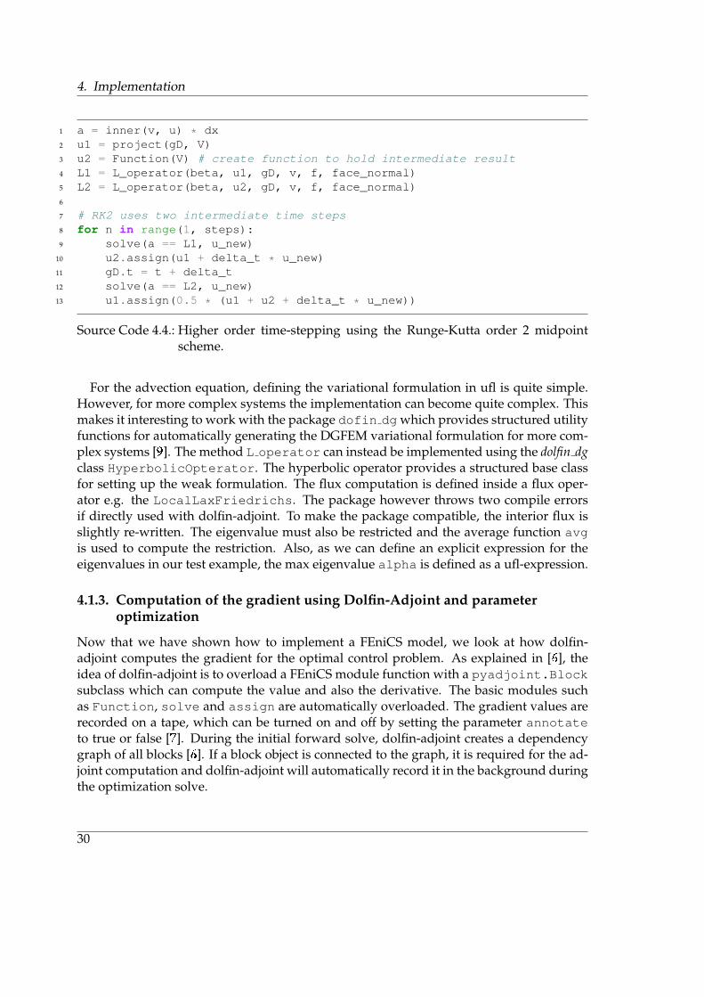
For the advection equation, defining the variational formulation in ufl is quite simple.However, for more complex systems the implementation can become quite complex. Thismakes it interesting to work with the package dofin dg which provides structured utilityfunctions for automatically generating the DGFEM variational formulation for more com-plex systems [9

.

]. The method L operator can instead be implemented using the dolfin dgclass HyperbolicOpterator. The hyperbolic operator provides a structured base classfor setting up the weak formulation. The flux computation is defined inside a flux oper-ator e.g. the LocalLaxFriedrichs. The package however throws two compile errorsif directly used with dolfin-adjoint. To make the package compatible, the interior flux isslightly re-written. The eigenvalue must also be restricted and the average function avgis used to compute the restriction. Also, as we can define an explicit expression for theeigenvalues in our test example, the max eigenvalue alpha is defined as a ufl-expression.

4.1.3. Computation of the gradient using Dolfin-Adjoint and parameteroptimization

Now that we have shown how to implement a FEniCS model, we look at how dolfin-adjoint computes the gradient for the optimal control problem. As explained in [6

.

], theidea of dolfin-adjoint is to overload a FEniCS module function with a pyadjoint.Blocksubclass which can compute the value and also the derivative. The basic modules suchas Function, solve and assign are automatically overloaded. The gradient values arerecorded on a tape, which can be turned on and off by setting the parameter annotateto true or false [7

.

]. During the initial forward solve, dolfin-adjoint creates a dependencygraph of all blocks [6

.

]. If a block object is connected to the graph, it is required for the ad-joint computation and dolfin-adjoint will automatically record it in the background duringthe optimization solve.

30


1 class LocalLaxFriedrichsModified(ConvectiveFlux):2 def interior(self, F_c, u, n):3 return dot(avg(F_c(u)), n) + 0.5 * self.alpha('+') * jump(u)4 def exterior(self, F_c, u_p, u_m, n):5 return 0.5 * (dot(F_c(u_p), n) + dot(F_c(u_m), n) /6 + self.alpha * (u_p - u_m))7

8 # operator derived from dolfin_dg base class9 class ElasticOperatorLOH1(HyperbolicOperatorModified):

10 ...11 def F_c(self, U):12 sig11, sig22, sig12, u, v = U[0], U[1], U[2], U[3], U[4]13 return as_matrix([[-(self.lam+2*self.mu)*u,-self.lam*v],14 [-self.lam*u,-(self.lam + 2*self.mu) * v],15 [-self.mu*v,-self.mu*u],16 [-(sig11/self.rho), -(sig12/self.rho)],17 [-(sig12/self.rho), -(sig22/self.rho)]])18

19 def __init__(self, mesh_, V, bcs, parameters):20 self.parameters = parameters21 self.domain_mesh = mesh_22 self.lam, self.mu, self.rho = get_expressions(parameters)23

24 HyperbolicOperatorModified.__init__(self, mesh_, V, bcs,25 self.F_c, LocalLaxFriedrichsModified(parameters))26 ...27 elasticOp = LOH1Operator(unit_mesh, V, DGDirichletBC(ds, gD),parameters)28 F = elasticOp.generate_fem_formulation(u, v) # auto-generated DGFEM29 F += dot((1 / dt) * (u - u1), v) * dx # add time discretization30 F -= inner(f, v) * dx

Source Code 4.5.: The LOH1Operator is derived from the base class Hyperbolic-Operator which is provided by dolfin dg [9

.

]. The classesHyperbolicOperator and LocalLaxFriedrichs are only slightlymodified to use a user defined expression as maximum eigenvalue,which is also restricted for the inner flux approximation.

In order to compute the derivative of the cost function J , some modifications to the FEn-iCS code have to be made. In the following section we use the basic setup for a parameteroptimization problem given in [7

.

]. The code listing (4.6

.

) show the basic setup for a param-eter optimization. The dolfin-adjoint object Control is used to define the optimizationparameter. Then the forward solve method has to be run once, so that dolfin-adjoint canrecord the annotated operations. The cost function J can be defined using the assemblemethod. If the cost function includes the integral over time, the evaluation over the do-

31

4. Implementation

main has to be done inside the forward solve at every time step, recorded in a python listwhich can after the time stepping be integrated over time [7

.

]. The minimize method callsthe scipy optimization routines e.g. the standard is the quasi newton method L-BFGS-B[27

.

]. For a user-defined expression the changes can not automatically be traced and dolfin-adjoint requires the list of dependencies together with the user defined derivatives of theexpression with respect to each dependency. We use the same solution approach for sucha case given in the documentation example [28

.

]. For example, the Lame parameter ρ of theLOH1 problem is formulated as a user-expression using a switch case as the value of thedensity changes depending on x being in the layer or in the half space. This means the ex-pression is dependent on the two FEniCS constants rho layer and rho hs (half-space).As the derivative with respect to the layer depth is not defined, the dependency is notadded but also cannot be used as a control variable. A solution would be to approximatethe step function with a smooth function to ensure that the derivative w.r.t. the layer depthis well defined.

1 control = Control(rho_layer) # optimization parameter2 u_sol = forward(..) # initial run of forward model to record adjoint3

4 J = assemble(inner(u_sol, u_sol) * dx) # Cost function definition5 J_hat = ReducedFunctional(J, control)6 # interface to scipy optimization routine7 opt_res = minimize(J_hat, method="L-BFGS-B", ftol=1.0e-8,8 options=...)

Source Code 4.6.: Basic dolfin-adjoint set up for a parameter optimization [7

.

].

The code for the parameter optimization in listing (4.6

.

), makes the following steps:

1. Define a control variable for the optimization parameter

2. Run the forward model once so that dolfin-adjoint can create a dependency graph

3. Define the cost function J as the squared difference between the initial forward so-lution and the measurements

4. Compute the derivative J with respect to the optimization parameter variable

5. Determine the reduced functional J

6. Start the optimization routine which will use the forward model to compute the costfunction J in every step and its derivative

32

4.2. TerraDG using Julia

1 rho = Expression("x[1] >= divide ? rho_layer : rho_hs",2 degree=1, name='rho_exp', divide=divide,3 rho_layer=rho_layer, rho_hs=rho_hs)4

5 rho.dependencies = [rho_layer, rho_hs] # add dependencies and derivatives6 d1 = Expression("x[1] >= divide ? 1.0 : 0.0", divide=divide, degree=1)7 d2 = Expression(...)8 rho.user_defined_derivatives = rho_layer: d1, rho_hs: d2

Source Code 4.7.: Dolfin-adjoint modifications: providing the dependency list with thecorresponding user defined derivatives for an expression [21

.

].


For a comparison, we extend the discontinuous Galerkin solver TerraDG, which was pro-vided by [3

.

] with an adjoint solver. For comparison we implement two different ap-proaches for computing the total derivative. A short overview of both approaches is givenin the following:

1. differentiate-first-then-discretize:

The adjoint equation is derived analytically via the Lagrangian approach. The for-ward equation and the adjoint equation are then discretized using the DiscontinuousGalerkin method. The discrete equations are then solved using TerraDG [3

.

]. The to-tal derivative is computed by the integral formulation also derived analytically usingthe Lagrangian function.

2. discretize-first-then-differentiate:

The cost function J and the PDE model F are first discretized using the Discontin-uous Galerkin method. The DG-solver TerraDG is used to solve the forward modeland compute the cost function. The total derivative is then computed by applyingautomatic-differentiation (AD) to the solver methods.

The advection equation is already implemented as a test equation in TerraDG. We addthe elastic wave equation following the general TerraDG structure given by [3

.

]. For everyequation the method evaluate flux() has to be provided, which for the elastic waveequation is defined according to the equation system (2.7

.

). The specified traction at theboundary is set to be zero and is implemented following the definition given in (2.9

.

).

4.2.1. Differentiate-first-then-discretize

For the differentiate-first-then-discretize ansatz, the adjoint equation is implemented the sameway as the forward system. For the advection equation we derived the analytical adjoint

33

4. Implementation

equation in (3.19a

.

) as

−∂Λ

∂t− β∇Λ = γ1(φ− Φ) (T, 0)× Ω

Λ = 0 (T, 0)× Γ

Λ = γ2(φ |t=T −Φ |t=T ) Ω at t = T.

and analytical gradient formulation as

DJ

Dβ=

∫Ω

∫ T

0Λ · φβ dtdΩ.

This is the gradient when computing the cost using the time tracking cost functional JT asis given in (3.1

.

). If the cost is computed only at the final time using JC as defined in (6.1

.

),the source term of the adjoint equation becomes zero and the total derivative becomes

DJ

Dβ=

∫Ω

Λ |t=T ·φβ |t=T dtdΩ.

During the forward solve we store the difference (φ − Φ) in every time step and can thenuse it to compute the source term of the adjoint equation. In the reverse solve the recordedvalues are used to compute the adjoint equation. To solve the advection equation with asource term, we use the Fractional-Step Method as shown in [8

.

]. First the homogeneousPDE

Λ∗t +∇ · F (Λ∗) = 0 (4.3)

then the ODE equationΛt = γ1(Λ∗ − Φ) (4.4)

with the source term as the right hand side. In TerraDG we solve the ODE using Euler timestepping, following the example given in [8

.

]. For the derivation of the analytical adjointequation we assumed that the boundary g is independent of the parameter and its deriva-tive with respect to the parameter is zero. As we apply the exact solution at the boundaryfor the test example, this condition is slightly different. For the reverse adjoint computationwe assume that the boundary stays the same and apply the periodic boundary conditionto the homogeneous adjoint PDE system.

Once the adjoint equation is computed, the gradient can be computed using the derivedanalytical integral formulations. However, the analytical formulation includes the solutionof the sensitivity equation φβ . We compute this during the forward solve using a simpleFinite Differences approximation. This means that the forward model solves the advectionequation twice: φ(β) and φ(β+ε). The reverse adjoint solve also solves one PDE advectionequation. In total, we require three PDE solves to compute the gradient. In theory, weshould also be able to use the right side of the Equation 3.21a

.

to replace the sensitivityderivative.

34


For large systems or long time simulations storing the forward solutions at every timestep would of course quickly become infeasible memory wise. A better approach is to usea check pointing algorithm such as [29

.

]. The main idea of these are to stores the solutiononly at a few optimally placed check points and can use these to compute the reverse solvemore efficiently. As check pointing is not implemented for the adjoint solver, we restrictour self to short simulation times and smaller test sizes.

4.2.2. Discretize-first-then-differentiate using AD

The general approach of AD is to decompose the code of a function into the most elemen-tary operations and functions for which the analytic derivative can be computed [30

.

]. ADthen computes the derivative of a function by applying the chain rule using ether forward-mode or reverse-mode. Before explaining how AD is applied to the DG code TerraDG, welook at a simple forward AD example to understand the general approach.

Forward mode automatic differentiation (AD)

The simple function f = sin(2π(x1−βt)) which can be considered as a composite functionof the most basic operations such as sin, cos or +/∗ [30

.

]. We follow the same steps as forthe example in [30

.

]. Equation (4.5

.

) shows the basic operations of f in the left column andthe derivative of each operation on the right.

z1 = x z′1 = x′

z2 = β z′2 = β′

z3 = t · z2 z′3 = t · z′2 (4.5)z4 = (z1 − z3) z′4 = (z′1 − z′3)

z5 = sin(2πz4) z′5 = cos(2πz4) · 2π · z′4

Starting from the most outside composite derivative, the complete derivative is put to-gether in one forward sweep per parameter. If we vary the function f with respect to x,then in equation (4.5

.

) we would know that the derivatives are z′1 = x′ = 1 and z′2 = β′ = 0.This can be seen as setting a seed (1, 0), where only the derivative variable is one and allothers are zero [30

.

]. If the derivative fβ is to be computed, then the forward sweep is madewith (x′ = 0, β′ = 1).

fx = z5x fβ = z5β

= cos(2π · z4) · 2π · z′4x = cos(2π · z4) · 2π · z′4β= cos(2π(z1 − z3)) · 2π · (z′1x − z

′3x) = cos(2π(z1 − z3)) · 2π · (z′1β − z

′3β

) (4.6)

= cos(2π(z1 − t · z2)) · 2π · (1− t · 0) = cos(2π(z1 − t · z2)) · 2π · (0− t · 1)

= cos(2π(x− t · β)) · 2π = cos(2π(x− t · β)) · 2π · −t

35

4. Implementation

The Julia forward-mode AD package ForwardDiff uses the dual numbers approach,which transforms all numbers into a dual number containing the actual function value aand the derivative component b of the function as a second additional component [31

.

].Mathematically, the dual number approach for computing the derivative is defined as

f(a+

N∑i=1

biεi) = f(a) + f ′(a)

N∑i=1

biεi, (4.7)

where f is a elementary function for which the overloaded derivative is defined [31

.

]. Forthe type overloading to work, all data structures in the TerraDG code case which are usedin the gradient computation have to be changed to use the abstract super type Core.Realas this is also the super type of the ForwardDiff DualT,V<:Real,N<:Real. As shownin [31

.

], the Julia ForwardDiff package provides the three methods:

• derivative(f, x) for f(x) : R→ R

• gradient(f,x) for f(x1, ..., xn) : Rn → R

• jacobian(f,x) for f(x1, ..., xn) : Rn → Rn

Gradient computation using AD

The ansatz discretize-first-then-differentiate, means that the AD routines are applied to thediscrete implementations of the cost function and the DG implementation of the PDE.TerraDG already provides the routines for the PDE discretization and the forward timeloop. The cost function is easily computed using numerical quadrature as

J(φi, tk, β) =

γ1

2∆t

m∑k=0

∆xn∑i=1

(φki (β)− Φki (β))2 (4.8)

+γ2

2∆x

n∑i=1

(φmi (β)− Φmi (β))2. (4.9)

The computation of the total derivative can be computed following [15

.

] using AD is di-vided into the two main steps:

1. Forward solve:

a) Compute the forward solution φ of the PDE

b) Compute the partial derivatives ∂J∂φ , ∂F∂φ and ∂J

∂α ,∂F∂α using an AD routine

2. Backward solve:

a) Solve the adjoint equation (3.23

.

) for Λ

b) Compute the total derivative using (3.26

.

)

36


Computing the partials using AD

In order to compute the partial derivatives listed in step 1.b), the code functions must bepassed in the right shape to the ForwardDiff package. In the TerraDG code base, theunknown state variable φ is stored in the three dimensional array dofs. The first dimen-sion contains the basis function points, e.g. for order two this would result in ord = 4basis points. The second dimension gives the number of variables nvars of the PDE equa-tion. The third dimension now contains the cell values of the row-wise flattend two di-mensional discrete grid of length ndofs. Following the iterative scheme derived in (3.58

.

)using [15

.

] the two derivatives ∂Fk

∂φkat the dofs time level k and ∂Fk

∂φk−1 at the dofs timelevel (k − 1) have to be computed. For Euler time stepping, the method step computesdofs .+= dt * dofsupdate, where the dofsupdate is the update δφ computed by theTerraDG method evaluate rhs. As shown in (3.23

.

) the derivative at the new time levelk is independent of the discretization, being the diagonal matrix with 1/dt as a value.The derivative at time level (k − 1) depends on the discretization and needs to be com-puted using AD. The output of the dofs update method is the same size as the dofs arrayD = (ord × nvars × ndofs), meaning the forward differentiation method jacobian isrequired for the derivative. If the dofs array of size D is directly passed to the gradientas the argument x, then the computed derivative matrix would be a very large Jacobianmatrix of size (D × D). Many of the computed partials inside the Jacobian are howevernot wanted. For example, the a PDE with variables φ1, φ2 and φ3, the full Jacobian wouldcontain the cross derivatives between the variables e.g. ∂Fφ1

∂φ2. To compute only partials of

evaluate rhs for a given variable and basis function point with respect to only the corre-sponding section in the dofs vector, a wrapper method is required. As shown in the listing(4.1

.

), the methods simply reassembles the dofs matrix. However, the wrapper functioncan now be passed as the function handle to ForwardDiff.jacobian with an explicitorder and variable index, which means only that subsection of the dofs vector is used asx. The computed derivative matrix is also sparse, as was shown in (4.8

.

). The Jacobian isstored using SparseVectors and the computation is done only once per forward solve,as the derivative matrix does not change over the time levels. Using a similar wrapperfunction setup, the derivatives of J with respect to the dofs vector can be computed usingthe gradient AD routine.

With the functions for computing the partials defined, the main time loop is extended bytwo structs: one CostFunction containing the methods for computing the cost functionand AdjointPartials for computing the derivatives as explained above. The backwardsolve of the adjoint variable is computed using the iterative scheme (3.58

.

). The implemen-tation is straight forward: one time loop and inside two for loops over the order and thevariables. After the forward and backward solve is done, the total derivative can be com-puted using the formula derived in (3.23

.

), as the dot product of the vectors Λ and thederivative ∂F

∂α plus the derivative of the cost function w.r.t. the parameter α.

37

4. Implementation

1 function evaluate_rhs_diff_dofs(dofs, ..., var_idx, ord_idx, diff_dof)2

3 du, dofs_diff = similar(dofs), similar(dofs, size(dofs))4 du .= 0.05 for ord in 1:size(dofs)[1]6 for var in 1:size(dofs)[2]7 if ord == ord_idx && var == var_idx8 dofs_diff[ord_idx, var_idx, :] .= diff_dof9 else

10 dofs_diff[ord, var, :] .= dofs[ord, var,:]11 end12 end13 end14

15 f = (dofs_diff_, du_) -> evaluate_rhs(... dofs_diff_, ...)16 return (-1/dt).*dofs_diff[ord_idx,var_idx,:]17 -f(dofs_diff, du)[ord_idx,var_idx,:]18 end19

20 wrhs = ddof -> evaluate_rhs_diff_dofs(...)21 drhs_ddofs = (dofs,.., var, ord, ddof) -> jacobian(w, ddof)

Source Code 4.8.: Wrapper functions for the AD forward diff routines to avoid unneces-sary cross derivatives.

1 for ord in 1:order2 for var in 1:nvars3 if is_final_time4 tmp = sparse(self.drhsddofs(dofs, ...,5 var, ord, dofs[ord,var,:]))6 tmp[diagind(tmp)] .+= 1.0/dt7 tmp .*= (-1.0)8 self.A1_trans[ord, var] = transpose(tmp)9 end

10

11 # derivative of J w.r.t. dofs12 dJddofs_k[ord, var, :] = self.dJddofs(...,13 dofs[ord,var,:])14

15 # derivative of rhs w.r.t. parameter16 drhsdparams_k[ord, var, :] = t.*self.drhsdparams(...,17 parameters[var])18 end19 end

38

Part IV.

Results

39

5. Tests


Both the forward solution model and gradient can be checked with convergence tests.For the forward model we know the time-stepping order which must be achieved. Asthe LOH1 equation does not have a known analytic solution, we test the planar wave setup to verify that the solutions are computed correctly. To verify the gradient computed,we use the Taylor test routine provided by dolfin-adjoint [7

.

]. To check the gradient forthe advection equation example computed using the TerraDG implementation, we cancompare to the exact solution.

5.1.1. Test equation convergence rates

For the verification of the forward models, we compute the convergence rates and ordersusing the test cases where an analytical solution is given. For a Runge-Kutta time-steppingscheme with s stages, the convergence rate and the order are computed using

conv. rate =e1

e2conv. order =

log( e1e2 )

log(∆t1∆t2

)(5.1)

where e1 is the L2-error computed with step size ∆t1 and e2 is computed with half the stepsize ∆t2 = ∆t1

2 . For the advection equation (2.6

.

) the analytic solution was given as:

φ(t,x) = sin(2π(x− βxt)). (5.2)

We remind our self, that for the two dimensional planar wave problem we derived theanalytic solution as:

φ(t,x) =

−k sin(2π(x− cpt))(λ+ 2µ)−k sin(k(x− cpt))λ−k sin(k(x− cst))µcpk sin(k(x− cpt))csk sin(k(x− cst))

, (5.3)

where k = 2π and cp, cs are the wave speeds. Table (5.1

.

) shows the achieved convergencerates and orders for the advection equation. The mesh points in every iteration is doubled,in order to half the cell size ∆x / ∆y. For the advection equation we can therefore showthat the forward solver computes the solution correctly.

41

5. Tests

DF L2-error conv. rate conv. order96 0.00823414 1.99001704 0.99278079192 0.00412927 1.9940917 0.99573176384 0.00206826 1.99649125 0.99746675768 0.00103524 1.99785882 0.998454641536 0.00051797 1.99865656 0.99903059

(a) Runge-Kutta order 1

L2-error conv. rate conv. order0.00196984 3.98674329 1.995210710.00049292 3.99631422 1.998670020.00012326 3.99911332 1.999680163.082e-05 3.99971794 1.999898277.7e-06 3.99994363 1.99997967

(b) Runge-Kutta order 2

Table 5.1.: Convergence rates and orders of the Runge-Kutta time discretization scheme forthe advection equation.

For the elastic wave equation we at first faced some stability problems. In tests, we canalso see that the computation requires a very small time step. The CFL number suggestedin [12

.

] is 0.01 if the domain is divided into 7 or 8 number of cells. If we use the by [12

.

]recommended magnitude of the CFL condition, 0.01, we see that the numerical solutionconverge towards the exact solution. The second order Runke-Kutta convergence rate is≈ 3.63978 and with that clearly better than the first order scheme but not the exact conver-gence factor 4. The Figure 5.1

.

show the DG approximations of the different componentscompared to the exact solutions. However, the large number of time steps make the com-putation time for the non-optimized FEniCS model quite long.

(a) The stress component solutions when usinga time step of ∆t = 0.0003125.

(b) The velocity component solutions when us-ing a time step of ∆t = 0.0003125.

Figure 5.1.: DG approximation and exact solution for the planar elastic wave equation in2D. The plot shows a one dimensional slice at y=1/2. The CFL condition ischosen small enough, such that the approximation converges towards the exactsolution.

42


equation M D K dofs L2-error J

elastic planar 2D 8 1 1920 2 0.805048268826636 664.658074451846elastic planar 2D 16 1 7680 2 0.22118072435718 678.229438053766

Table 5.2.: Approximation L2-error for the elastic planar wave equation.

5.1.2. Gradient convergence rates

For testing the gradient computation, dolfin-adjoint provides a Taylor Test routine, as thetotal derivative DJ

Dα can also be approximated using the second order Taylor remainder [2

.

].This test routine be used to can simply verify that the adjoint computation of dolfin-adjointis working correctly. If the Taylor test fails, it may be that the dependencies of the controlvariable are not properly linked. For a second order approximation

TO(2) = |J(α+ hδ)− J − h∇Jδ|, (5.4)

the residual should decrees by a factor of four each time the perturbations δ is halved.For the FEniCS LOH1 and advection models the Taylor test routine is used to check ifthe gradient computation achieves the correct second order convergence. The step size hshould ideally be chosen to be of the same magnitude as the control variable [7

.

]. Table (5.3

.

)shows a selection of different optimization settings and the achieved convergence orders.For the elastic wave test example, the planar wave setting, the Taylor test was not made, asthe computation time for that model is quite large. The problem for this example case is,that an increasing number of time steps significantly increases the computation time whencomputing the gradient with dolfin-adjoint.

Equation DF D K control mean convergence rateadvection-2D 384 1 rk1 βx 1.99703241430964advection-2D 768 2 rk1 βx 1.99753701617741Advection 2D 384 1 rk2 βx 1.99787865647545Advection 2D 768 2 rk2 βx 1.99792167791555

LOH1 7680 1 rk1 sx 1.99996326615342LOH1 15360 2 rk1 sx 1.99996620106436

Table 5.3.: The FEniCS Taylor test routine convergence orders can be used to validate thegradient computed for the test equations. The convergence order must be two,other wise the gradient computation still contains errors. The type of cost func-tion used was the controllability functional JC .

5.1.3. Convergence test for the TerraDG adjoint solver

In general, the cost functional depends on the parameters α directly and indirectly via thestate vector. The reduced cost functional J , re-formulates the cost functional so that the

43

5. Tests

indirect dependency on parameters α become a direct dependencies [2

.

]. To get comparisongradient approximation, we can implement the simple FD scheme

∂J

∂β≈ J(β + ε)− J(β − ε)

2ε

for computing the gradient using the analytic solution of φ [2

.

]. Table (5.4

.

) shows the ap-proximated gradients.

N J type J DJ100 JC 0.2048959051063637 2.5161692718895927200 JC 0.20550163948006359 2.5288771975051914400 JC 0.2058045066669135 2.53523116031299880 JT 0.28404712098242624 3.513347722958295120 JT 0.2822130575671631 3.4964016316303597200 JT 0.2807607164159079 3.482960072540482

Table 5.4.: Finite Difference approximation of the Reduced functional gradient ∂J/∂β.

We can simply check if the Finite Difference method computes the correct gradientvalue. If we consider the controllability cost function

JC =1

2

∫Ω

(φ(β)− Φ)2dx, (5.5)

we can insert the analytic solution and can thus write the cost functional in reduced form.The gradient of JC can be derived analytically using the chain rule and then computedusing numerical quadrature as

dJCdβ

=

∫ 1

0[sin(2π(x− βtn))− sin(2π(x− βtn))] (5.6)

· (−2πtn cos(2π(x− βtn))) dx

≈ 2.541636269831977

Comparison to the gradient values computed using AD

In Table (5.5

.

) we see the gradient values computed using the AD adjoint implementationin TerraDG. For the controllability cost functional the computed values seem to convergetowards the FD solution. However, as the forward model suffers from strong numericaldiffusion, the gradient value is of course affected by this. We can also see the loss in accu-racy in the cost function value JC . To overcome the problem of numerical diffusion, onecould simply increase the DG order. However, when computing the adjoint using higher

44


(a) Adjoint for JC (b) Adjoint for JT

Figure 5.2.: Solutions to the adjoint equation computed using automatic-differentiation.The Controllability cost functional J only computes the cost at the final timestep, making the adjoint an homogeneous advection equation. The Timetrack-ing cost functional computes the cost over the entire time domain, resulting ina source term for the adjoint equation.

M DG RK L2-error forward sol. J type J DJ30 1 RK1 0.105087624845139 JC 0.179632166602784 2.1109095656355760 1 RK1 0.054493340271583 JC 0.191903487169665 2.3133426493130930 1 RK1 0.105087624845139 JT 0.244841372899244 3.4792171178687660 1 RK1 0.054493340271583 JT 0.259702163311143 3.79371286885047

Table 5.5.: Gradients computed using TerraDG using the AD ansatz.

order DG elements, the adjoint solution becomes zero as can be seen in Figure (5.3

.

). Theadjoint computation should stay exact the same for higher order. No literature examplecould be found, regarding an implementation of an adjoint solver using automatic differ-entiation and higher order DG. A possible cause for the problem could be that the higherorder volume term is not correctly differentiated by the AD package. If more time for theproject been available, the results could have been compared with a different AD packagese.g. reverse mode AD. The gradient for the Time tracking cost functional JT computed us-ing AD in TerraDG also contains a large error when comparing to the Finite Differencesapproximation. This could be due to the stronger effects of numerical diffusion when com-puting the cost over the complete time domain or could of course be an indicator that theadjoint is not jet computed correctly. Further test would have to be made here. Especially,a test using higher order DG elements would be good, to get a better forward solutionapproximation.

The AD approach currently uses the sequential forward solver. As there are still issueswith the gradient computation, code optimizations where not jet made. We can still look at

45

5. Tests

where in the adjoint solver the most compute time goes to. For the AD approach the mostexpensive operation is computing the adjoint system matrix ∂F

∂φ , as it has (n2 × n2). Thecomputation time for the computed gradients are listed in Table (5.6

.

). The run time of theAD adjoint solver in TerraDG is dominated by the computation of the gradient matrix ∂F

∂φ .The time and memory measurement of the AD computation shows how costly computingthe full Jacobian matrix is. For twice as many degrees of freedom, the computation time isapprox. 10 times as long. For this reason, using higher order DG might be advantageous.As the cause for the higher order solution converging towards zero could not be found jet,this theory could not be checked.

Despite the large error in the gradient, it is still possible to use the computed gradientin a Optimal Control Optimization. We use the simple the advection equation test case:φ(x, t) = sin(2π(x − βt)). The mock measurements are created with the velocity β = 0.1.Starting with the initial guess β0 = 0.25, the optimization convergences in five iterationstowards ≈ 0.09976115231365439.

solver step M time and storage measurementControllability JC 30

dFdphi 12.294389 s (103.00 M alloc: 6.435 GiB, 10.01% gc t)forward 58.433055 s (304.08 M alloc: 12.601 GiB, 5.26% gc t)reverse 5.533887 s (11.10 M alloc: 844.495 MiB, 5.06% gc t)

Controllability JC 60dFdphi 121.994853 s (1.57 G alloc: 98.896 GiB, 14.03% gc time)forward 260.195863 s (2.78 G alloc: 129.595 GiB, 9.10% gc time)reverse 33.423291 s (79.03 M alloc: 16.776 GiB, 4.13% gc time)

Time Tracking JT 60dFdphi 132.404556 s (1.56 G alloc: 98.622 GiB, 11.62% gc time)forward 366.741602 s (4.20 G alloc: 213.477 GiB, 11.23% gc time)reverse 8.740723 s (81.41 M alloc: 2.395 GiB, 8.20% gc time)

Table 5.6.: The run time of the AD adjoint solver in TerraDG is dominated by the compu-tation of the gradient matrix ∂F

∂φ . The time and memory measurement of theAD computation shows how costly computing the full jacobian matrix is. Fordouble the number of cells, the computation time is approx. 14 times as long.

Comparison to the gradient values computed using the Differentiate-then-discretizeAnsatz

The second adjoint method for computing the gradient is the differentiate-then-discretizeapproach. The computed adjoint equation when using the Time tracking cost functionalJT can be seen in Figure (5.4

.

). The adjoint equation solution is nearly the same as forthe AD computation, however the solutions differ in the magnitude. This is because both

46


Figure 5.3.: The adjoint equation computed using ForwardDiff AD becomes zero, whenswitching to higher order DG element. The exact cause for this error couldnot be determined. The correct adjoint should also be a sinus curve which isadvected to the left.

methods use a differently scaled terminal condition on the adjoint. The AD Ansatz usesΛT = ∆t∂J∂φ , while in the differentiate then discretize Ansatz we solve the adjoint equationusing the TerraDG solver. We remind ourself, that the adjoint of the advection equationlooks like

−∂Λ

∂t− β∇Λ = γ1(φ− Φ) (T, 0)× Ω

and uses the terminal condition Λ = γ2(φ |t=T −Φ |t=T ). The gradient values computedusing the second ansatz in TerraDG, are listed in Table (5.7

.

). We see the same again: theerror in the gradient is quite high, mostly due to numerical diffusion.

M error forward J DJ30 0.10508762484513891 0.244841372899244 3.02722491569337160 0.05449334027158299 0.259702163311143 3.1923370015307433

Table 5.7.: Gradients computed using the differentiate-then-discretize using TerraDG for theTimetracking cost functional. The error of the forward

Just like for the AD Ansatz, the implementation for the differentiate-then-discretize isnot yet optimized for run time or memory requirements. In Table 5.8

.

we can see the mem-ory and run time for the sequential forward and reverse models. The forward solve timeincreases much stronger than the reverse solve with increasing degrees of freedom. Thiscould be due to the storage of the forward solutions. As mentioned before, a check point-ing algorithm such as [29

.

] could improve the performance of the adjoint solver.

47

5. Tests

solver step M Time and memory measurementsforward 15 30.708099 seconds (63.73 M alloc:: 2.677 GiB, 3.80% gc time)reverse 15 4.652970 seconds (10.92 M alloc: 355.035 MiB, 2.95% gc time)forward 30 46.934199 seconds (167.45 M alloc:: 5.099 GiB, 3.87% gc time)reverse 30 9.411440 seconds (59.81 M alloc:: 1.473 GiB, 4.21% gc time)forward 60 177.796064 seconds (986.43 M alloc:: 24.047 GiB, 5.02% gc time)reverse 60 54.219801 seconds (448.45 M alloc:: 10.386 GiB, 5.10% gc time)

Table 5.8.: Time and memory measurements for the gradient computation using thedifferentiate-then-discretize Ansatz in TerraDG and a Time Tracking cost func-tional JT . The allocations are given in M

Figure 5.4.: The adjoint computed using the differentiate-then-discretize approach whichsolves the discrete analytical adjoint equation using the same solver as the for-ward problem. For the solver, the time stepping is not reverse but the advectionvelocity is reversed instead with the time direction remaining forward in timestepping.

5.2. Visualization

5.2.1. Plots of the approximated solutions

It is always a good correctness check to plot the PDE model solution. For the advectionequation we can run the simple Parameter Optimization Problem as explained previously.We plot the solutions in every iteration, as shown in Figure 5.5

.

. For the LOH1 we can seethe computed solution in Figure (5.6

.

) and (5.7

.

).

5.2.2. Graph visualization methods in FEniCS

To visualize how dolfin-adjoint internally processes a given model internally, it is possibleto create a graph showing the basic operations and dependencies using Graphviz (or Ten-

48

5.2. Visualization

Figure 5.5.: Correctness check: Plotting the solution of the advection equation, computedusing the FEniCS model. The plots are a line plot over x at y=0.5. At eachiteration, the new forward solution is plotted. As we can see, the optimizationconverges quite quickly towards the correct measurement data.

Figure 5.6.: Stress component solution of the LOH1 at the final time t = 1.0. The initialdisturbance is set as a Gaussian curve as shown in equation 2.15

.

. The layerregion is 1[km] deep from the top boundary. The source origin is at (26km,32km) We can see that the zero boundary condition in φ12 is still approximatelyfull filled.

Figure 5.7.: The velocity components of the LOH1 equation at the final time t=0. The layerregion is 1[km] deep from the top boundary. The source origin is at (26km,32km).

49

5. Tests

sorFlow) [7

.

]. By adding the two visualization method callstape = get_working_tape()

tape.visualize('graph.dot')

all connections are recorded in a dot file which is visualized in Figure (5.8

.

). The graphshows the simulation flow for two time levels and the correct dependency of the flowvelocity beta vec on the x and y component which can be used as control variables.

Figure 5.8.: Visualization of the dependencies graph generated by dolfin-adjoint showingtwo time steps of a forward solve.

50



In this section we now want to use the adjoint solver to solve optimal control problems.The main model settings are: DG-order D = [1, 2], mesh sizeM = [8, 16] and Runge-KuttaorderK = [1, 2]. The degrees of freedom of the PDE solver can be computed as df = D·M2.For the example optimizations the Quasi-Newton minimization routine L-BFGS-B is used.

6.1.1. Optimization example 1: Initial disturbance origin of LOH1

The LOH1 setup simulates a basic earthquake scenario, where the initial disturbance islocated in the half-space with the origin sm = (sx, sy). Mock measurements are createdusing the origin sm = (26, 32) to act as placeholder for real sensor data. We can use theexact origin point of the measured data to check the correctness of the optimization. Forthe first optimization example, the controllability cost function JC

JC(φ, α) =γ2

2

∫Ω

(φ |t=T −Φ |t=T )2dΩ. (6.1)

as defined in (6.1

.

) is used to determine the earthquake origin (sx, sy) of the LOH1 model.We further restrict the optimization by passing the domain boundaries as optimizationbounds. The mock measurements φm are computed using the same DG-order and meshpoints as the simulated solution. To compare with a more realistic cost function setting, weuse the sensor cost function JS , where the measurements are taken at a limited number ofreceiver points. For the computation in FEniCS we define the discrete sensor cost functionas:

JS(φ, α) =1

2

M∑k=0

∫Γtop

(φ(xi,j , t)− Φ(xi, t))2dΓtopdt (6.2)

+

∫Γtop

(φ(xi,j , T )− Φ(xi, T )2dΓtop. (6.3)

For this example, we compute the cost function JS over the points at the top boundaryΓtop = [x, y = 33]. To see the stabilization effect of the second additional integral termat the final time T , we also do the optimization with γ2 = 0 and name the resulting costfunction for simplicity JK . Table (6.1

.

) and Figures show the optimization results for thesolver parameters DG order D, number of cells both directions M and the Runge-Kutta

51


Figure 6.1.: Comparison of the controllability cost functional value JC where the cost func-tional is computed over the entire domain and the sensor cost functional valueJS , where the cost is computed only at the upper boundary but over the entiretime domain. .

order K. As expected, the controllability cost functional JC performs best. For the sensorcost functional JS to achieve a similar error, second order DG-element and second ordertime stepping is required. In Figure (6.2

.

) we see the cost over the optimization iterations forthe controllability cost functional and the sensor cost functional. As expected, JC requiresmore iterations to reduce to zero. The sensor cost functional value drops only very slightlyat the beginning of the iteration but then stays constant.

Figure 6.2.: Error in the optimization parameters (sx, sy) in the x and y direction. The costfunctional JC computes the cost over the entire computation domain Ω. Theerrors on the right are for the sensor cost function JS . We see that the opti-mization still performs quite well, even if we compute the cost only at the topboundary over the entire time domain.

The error graphs, as shown in (6.2

.

), show how well the optimization routine estimates

52


Figure 6.3.: Variation of the initial guess for the Optimal Control Problem. One can seethat the optimization may not converge, if the initial error is too large. Thevariations where computed for a course grid ofM = 8, K = RK1 and D = 1.

the optimal parameter. For the cost functional the error decreases more slowly but thendrops lower than the sensor cost functional. For JS to achieve the same error as in JC ,higher order DG element and higher order time stepping has to be chosen. The gradientdevelopment over the iterations is shown in (6.4

.

).

Figure 6.4.: Gradient of the cost functional for the optimization parameters (sx, sy).

The initial value could of course have a large impact on the convergence towards thecorrect origin point. As a test, we start a Optimal Control Optimization with differentinitial values. The initial values are depicted in Figure (6.3

.

), where each initial start pointis coloured, orange for convergence and blue for divergence. The final error is noted nextto the iteration starting points. We can also compare to the cost functional JK , where wedid not add the integral at the final time again. According to [1

.

], it can acct as a stabilizationterm. In Table (6.1

.

), we can see that the is always higher apart from when using the coarsestmodel settings (7680 dofs with RK1).

53


M D dofs K type J Tit final error opt param16 1 7680 RK1 JC 16 0.04188 (25.96357 32.02065)16 1 7680 RK1 JK 10 1.0779 (25.08867 32.57563)16 1 7680 RK1 JS 11 5.74064 (24.88569 26.36854)16 1 7680 RK2 JC 18 0.01639 (25.98592 32.00838)16 1 7680 RK2 JK 36 0.72785 (25.79932 31.30036)16 1 7680 RK2 JS 24 0.33689 (25.72567 32.19555)16 2 15360 RK1 JC 17 0.01011 (25.99201 32.00619)16 2 15360 RK1 JK 11 0.59522 (26.01895 31.40508)16 2 15360 RK1 JS 10 0.34118 (25.9973 31.65883)16 2 15360 RK2 JC 18 0.00283 (25.99768 32.00162)16 2 15360 RK2 JK 21 0.76624 (26.04455 31.23506)16 2 15360 RK2 JS 11 0.44638 (25.99382 31.55366)

Table 6.1.: Optimal Control Optimization results: detection of the origin point sm of the ini-tial disturbance for the LOH1 equation. We compare three different cost func-tions: JC which computes the cost over the complete domain but only at thefinal time T=1. The sensor cost function JK computes the cost only over the topboundary. The stabilized sensor cost function JS which adds the integral overthe top boundary at the final time as a stabilization term.

54

Part V.

Conclusion

55

7. Conclusion

We looked at two different approaches for computing the adjoint and the gradient. TheDifferentiate-then-Discretize Approach requires the derivation of the analytical adjoint equa-tion. For the simple advection equation example, the derivation is still relatively simple.However, deriving the the Lagrangian function with respect to the state vector can quicklybecome quite complex for larger equation systems as for example the elastic wave equa-tion. Not for every PDE equation it is possible to derive an adjoint equation. We imple-mented this approach as a prototype adjoint solver for the advection equation in TerraDG[3

.

]. We saw that the gradient computation requires two additional forward solves andtherefore is quite costly. The next step would be to optimize the adjoint computation usingthe check pointing algorithm suggested in [29

.

]. This would reduce the memory require-ments and allow the computation of larger systems and longer simulation times.

We then looked into the Discretize-then-Differentiate ansatz, where Automatic Differenti-ation is used to compute the gradient of a implemented forward solver. We decided to firsttest the Julia ForwardDiff package [31

.

] in a second prototype adjoint solver in TerraDG.The AD package is quite easy to use but perhaps not the most efficient. For example, itwould be interesting to compare the performance to a package using reverse AD. In gen-eral, reverse AD is more efficient if the input dimension is larger than the output dimension[30

.

]. When computing the gradient for a large number of parameters, this might becomemore efficient. The implemented AD adjoint solver prototype could also not completely betested as the adjoint becomes zero when switching to higher order DG-elements. It is notquite clear what causes this problem. A suspicion, that could how ever not jet be proven,is that the volume term somehow is not correctly differentiated. As shown in the ChapterTests, the adjoint solution and gradient can still be computed but with a high approxima-tion error. Further tests have to be done to resolve the error for higher order DG and thenalso do a comparison between first order and higher order gradient computations.

The second goal was to test the dolfin-adjoint package, which uses the finite elementsolver FEniCS [6

.

], [4

.

]. The software packages we completely new to me and uses a verydifferent approach to the standard numerical PDE solver. With the python interface ofFEniCS one can directly implement the weak formulation of a forward model using UFL[19

.

]. If one has previously not worked with such formulations but rather with the standarddiscrete numerical solvers setups, using the UFL language requires some re-accustoming.With a large number of FEniCS examples and tutorials available, it is quite simple to im-plement a basic PDE model. The focus of most tutorials are however more elliptic PDEequations. Also the implementation of boundary conditions can be quite different.

As an example optimal control problem we tried determining the origin of the initial

57

7. Conclusion

disturbance in the LOH1 equation [14

.

]. This showed that the FEniCS and dolfin-adjointmodel work quite well. The origin can be detected, even when using a cost functional thatcomputes the cost only at the top boundary over the complete time domain. In general theFEniCS code still has a lot of room for improvement, especially run time optimizations.For finer meshes in combination with higher order DG elements, the FEniCS solvers arestill too slow to be able to use them in an optimization routine. This of course would bethe next step for improving the solvers. For example, if one can avoiding the assembly ofthe system matrix in every time loop, this would decrease the forward computation timeand with that also the backward solver speed [21

.

].

58

59

Bibliography

[1] M. D. Gunzburger, Perspectives in flow control and optimization, ser. Advances in designand control. Society for Industrial and Applied Mathematics.

[2] P. E. Farrell. Mathematical background: adjoints and their applications. [Online].Available: http://www.dolfin-adjoint.org/en/latest/documentation/maths/index.html#dolfin-adjoint-mathematical-background

.

[3] L. Krenz. Terradg. [Online]. Available: https://github.com/krenzland/TerraDG.jl

.

[4] M. S. Alnæs, J. Blechta, J. Hake, A. Johansson, B. Kehlet, A. Logg, C. Richardson,J. Ring, M. E. Rognes, and G. N. Wells, “The fenics project version 1.5,” Archive ofNumerical Software, vol. 3, no. 100, 2015.

[5] A. Logg, K.-A. Mardal, G. N. Wells et al., Automated Solution of Differential Equations bythe Finite Element Method. Springer, 2012.

[6] S. K. Mitusch, S. W. Funke, and J. S. Dokken, “dolfin-adjoint 2018.1: automatedadjoints for fenics and firedrake,” Journal of Open Source Software, vol. 4, no. 38, p.1292, 2019. [Online]. Available: https://doi.org/10.21105/joss.01292

.

[7] F. S. W. Farrell, Patrick E. Mathematical background: adjoints and their applications.[Online]. Available: http://www.dolfin-adjoint.org/en/latest/documentation/maths/index.html#dolfin-adjoint-mathematical-background

.

[8] R. J. LeVeque, Finite volume methods for hyperbolic problems, ser. Cambridge texts inapplied mathematics. Cambridge University Press.

[9] P. Houston and N. Sime, “Automatic symbolic computation for discontinuousgalerkin finite element methods.” [Online]. Available: http://arxiv.org/abs/1804.02338

.

[10] D. Corrigan, L. Fullard, and T. Lynch, “Advection problems with spatially varyingvelocity fields: 1d and 2d analytical and numerical solutions,” vol. 146, no. 8,p. 04020053, publisher: American Society of Civil Engineers. [Online]. Available:https://ascelibrary.org/doi/abs/10.1061/%28ASCE%29HY.1943-7900.0001782

.

[11] A. Fichtner, Full Seismic Waveform Modelling and Inversion.

61

http://www.dolfin-adjoint.org/en/latest/documentation/maths/index.html#dolfin-adjoint-mathematical-background


https://github.com/krenzland/TerraDG.jl

https://doi.org/10.21105/joss.01292



http://arxiv.org/abs/1804.02338

http://arxiv.org/abs/1804.02338

https://ascelibrary.org/doi/abs/10.1061/%28ASCE%29HY.1943-7900.0001782

Bibliography

[12] L. C. Wilcox, G. Stadler, C. Burstedde, and O. Ghattas, “A high-order discontinuousgalerkin method for wave propagation through coupled elasticacoustic media,” vol.229, no. 24, pp. 9373–9396. [Online]. Available: https://linkinghub.elsevier.com/retrieve/pii/S0021999110005024

.

[13] L. Krischer. Seismo-live. [Online]. Available: https://krischer.github.io/seismo live build/html/Earthquake%20Physics/DiscontinuousGalerkin/dg elastic physicalfluxes wrapper.html

.

[14] SISMOWINE. [Online]. Available: http://www.sismowine.org/index.html?page=model&mset=WP

.

[15] A. C. Duy, “An introduction to gradient computation by the discrete adjoint method,”p. 27.

[16] U. M. Ascher and L. R. Petzold, Computer Methods for Ordinary Differential Equationsand Differential-Algebraic Equations. SIAM, google-Books-ID: VL51G5JYYAYC.

[17] A. Logg and G. N. Wells, “Dolfin: Automated finite element computing,” ACM Trans-actions on Mathematical Software, vol. 37, no. 2, 2010.

[18] A. Logg, G. N. Wells, and J. Hake, DOLFIN: a C++/Python Finite Element Library.Springer, 2012, ch. 10.

[19] M. S. Alnæs, A. Logg, K. B. Ølgaard, M. E. Rognes, and G. N. Wells, “Unified formlanguage: A domain-specific language for weak formulations of partial differentialequations,” ACM Transactions on Mathematical Software, vol. 40, no. 2, 2014.

[20] M. S. Alnæs, UFL: a Finite Element Form Language. Springer, 2012, ch. 17.

[21] H. P. Langtangen and A. Logg, “Solving PDEs in python the FEniCS tutorial volumei,” p. 153.

[22] Kamensky. Lax-friedrichs flux for advection equation. [Online]. Available: https://fenicsproject.discourse.group/t/lax-friedrichs-flux-for-advection-equation/4647

.

[23] N.U. Form language unified form language (UFL) 2021.1.0 documentation.[Online]. Available: https://fenics.readthedocs.io/projects/ufl/en/latest/manual/form language.html

.

[24] J. Hake. fenics-project / dolfin / python / demo / undocumented /dg-advection-diffusion / demo dg-advection-diffusion.py bitbucket. [Online].Available: https://bitbucket.org/fenics-project/dolfin/src/master/python/demo/undocumented/dg-advection-diffusion/demo dg-advection-diffusion.py

.

[25] N.U. DG advection equation with upwinding firedrake documentation. [Online].Available: https://firedrakeproject.org/demos/DG advection.py.html

.

62

https://linkinghub.elsevier.com/retrieve/pii/S0021999110005024

https://linkinghub.elsevier.com/retrieve/pii/S0021999110005024

https://krischer.github.io/seismo_live_build/html/Earthquake%20Physics/DiscontinuousGalerkin/dg_elastic_physicalfluxes_wrapper.html



http://www.sismowine.org/index.html?page=model&mset=WP

http://www.sismowine.org/index.html?page=model&mset=WP

https://fenicsproject.discourse.group/t/lax-friedrichs-flux-for-advection-equation/4647

https://fenicsproject.discourse.group/t/lax-friedrichs-flux-for-advection-equation/4647

https://fenics.readthedocs.io/projects/ufl/en/latest/manual/form_language.html

https://fenics.readthedocs.io/projects/ufl/en/latest/manual/form_language.html

https://bitbucket.org/fenics-project/dolfin/src/master/python/demo/undocumented/dg-advection-diffusion/demo_dg-advection-diffusion.py

https://bitbucket.org/fenics-project/dolfin/src/master/python/demo/undocumented/dg-advection-diffusion/demo_dg-advection-diffusion.py

https://firedrakeproject.org/demos/DG_advection.py.html

Bibliography

[26] C.-W. Shu and S. Osher, “Efficient implementation of essentially non-oscillatoryshock-capturing schemes,” vol. 77, no. 2, pp. 439–471. [Online]. Available:https://linkinghub.elsevier.com/retrieve/pii/0021999188901775

.

[27] P. Virtanen, R. Gommers, T. E. Oliphant, M. Haberland, T. Reddy, D. Cournapeau,E. Burovski, P. Peterson, W. Weckesser, J. Bright, S. J. van der Walt, M. Brett, J. Wil-son, K. J. Millman, N. Mayorov, A. R. J. Nelson, E. Jones, R. Kern, E. Larson, C. J.Carey, I. Polat, Y. Feng, E. W. Moore, J. VanderPlas, D. Laxalde, J. Perktold, R. Cim-rman, I. Henriksen, E. A. Quintero, C. R. Harris, A. M. Archibald, A. H. Ribeiro,F. Pedregosa, P. van Mulbregt, and SciPy 1.0 Contributors, “SciPy 1.0: FundamentalAlgorithms for Scientific Computing in Python,” Nature Methods, vol. 17, pp. 261–272,2020.

[28] S. Vandekerckhove. Time-dependent optimal control of the linear scalar wave equa-tion. [Online]. Available: http://www.dolfin-adjoint.org/en/latest/documentation/maths/index.html#dolfin-adjoint-mathematical-background

.

[29] A. Griewank and A. Walther, “Algorithm 799: revolve: an implementation ofcheckpointing for the reverse or adjoint mode of computational differentiation,”vol. 26, no. 1, pp. 19–45. [Online]. Available: https://doi.org/10.1145/347837.347846

.

[30] N.U. Automatic differentiation. [Online]. Available: https://en.wikipedia.org/wiki/Automatic differentiation

.

[31] J. Revels, M. Lubin, and T. Papamarkou, “Forward-mode automatic differentiationin Julia,” arXiv:1607.07892 [cs.MS], 2016. [Online]. Available: https://arxiv.org/abs/1607.07892

.

63

https://linkinghub.elsevier.com/retrieve/pii/0021999188901775



https://doi.org/10.1145/347837.347846

https://en.wikipedia.org/wiki/Automatic_differentiation

https://en.wikipedia.org/wiki/Automatic_differentiation

https://arxiv.org/abs/1607.07892

https://arxiv.org/abs/1607.07892

Documents

Computational Science and Engineering (International