Embed Size (px)
Citation preview
Computational Reaction-Diffusion Analysis of Cellular Systems for Tissue Engineering and Quantitative Microscopy
by
Khamir H. Mehta
A dissertation submitted in partial fulfillment of the requirements for the degree of
Doctor of Philosophy (Chemical Engineering)
in The University of Michigan 2009
Doctoral Committee:
Professor Jennifer J. Linderman, Chair Professor Shuichi Takayama Professor Robert M. Ziff Assistant Professor Peter J. Woolf

© Khamir H. Mehta
2009

ii
Dedication
To my parents for their constant, unyielding, and unconditional support in whatever I have attempted, and whatever I will attempt

iii
Acknowledgements
I would like to express my deep gratitude to my thesis advisor, Professor Jennifer
Linderman, who has been a really wonderful mentor throughout my tenure as a graduate
student at Michigan. I take with me, not only the technical knowledge that I have
acquired during my numerous conversations with her, but also the wisdom of dealing
with situations that seem to be beyond my capabilities to handle before I joined the
department. I would also like to thank her for her guidance and especially her patience
with me, and I know much of it was tested during the past five years.
I would also like to thank my committee members, Professor Peter Woolf,
Professor Shuichi Takayama, and Professor Robert Ziff for all their help and guidance
during my thesis research. Peter, with his unique style, and infinite knowledge was a
constant source of inspiration and energy, and I have often relied upon him to help me
out with a tricky research situation. Professor Takayama has always been supportive of
my crazy schemes of developing mathematical theories, and I really owe him a lot for his
help and guidance on understanding the experimental side of my projects, not to mention
his help in bringing me up to date on the experimental aspects via meetings with his
graduate students. I owe my coming to Michigan for graduate studies to Professor Ziff;
He has been a great mentor and teacher, and I have learnt a lot from him. Every meeting
iv
with him has been inspirational, both in the doing good research, as well as lessons on
being better in life. He has been of great help in dealing with day-to-day issues of
graduate studies as well.
I would also like to thank the following faculty for their time and very useful
guidance at different stages of my dissertation research: Professor David Mooney,
Professor Sean Morrison, Professor Paul Krebsbach and Professor Robert Taichman. I
would especially like to thank Adam Hoppe, who was instrumental for motivating me
and supporting me for a project, which became a significant part of my thesis. All of my
knowledge of microscopy and FRET is due to his teaching. My time spent in his research
laboratory was as educationally enriching as it gets. I also acknowledge his help and
guidance, and my discussions with him have made my research better than my initial
plan.
I would like to acknowledge my teachers at UM, some of the courses here were
outstanding, and they fueled my desire to do better research. Special mention must go to
the following teachers; I found their course exceptionally educative and useful: Professor
Mike Solomon, Professor Mark Newman, Professor Robert Ziff, Professor Peter Woolf,
Professor Erdogan Gulari, and Professor James Rossmanith. I would also like to take this
opportunity to thank my teachers and mentors at Indian Institute of Science: Professor
Giridhar Madras, Professor Jayant Modak, Professor KS Gandhi, Professor Sanjeev
Gupta, Prof. V Kumaran, Professor Govind Rao and Professor Kesava Rao. I am greatly
indebted to them for making me as competent as I am today, and I don’t think I would
have achieved this much without their training. I owe immense gratitude for my advisor

v
at IISc, Professor Giridhar Madras who motivated and supported me in every step during
my bid for doctoral studies.
I would like to thank the support staff at the department for their timely and useful
help. Ms Susan Hamlin has been enormously helpful in getting all the required
paperwork done; I doubt if I would have been able to do it without her help. I also would
want to acknowledge the help from Mike Africa for computer support and Ruby Sowards
for help with other stuff. Special mention also must be made for Sam Straight in Adam
Hoppe’s lab for his help with servers for the FRET microscopy project.
I don’t think I would ever be able to find words to convey my gratitude for my
parents and my brother Pramit. They have been a constant source of strength, and
wherever I stood, I always found them to be on my side. I especially would want to
acknowledge their support during tough times, when nothing seemed to go right. I would
also like to thank my wife, Uditi, for being supportive, and keeping up with my ‘weird’
style of working and general mess that I created when working from home. She has been
a constant companion ever since she got here, and her support has been of immense help
in overcoming some of the stalemate situations that I have faced.
I have been truly blessed to have some of the best people as my friends. I would
really like to acknowledge the help of my schoolmates, especially those here in USA, for
their support and love. Ketan, Jigar, Jaimin, Jaysuryan, Hitendra -- I acknowledge the
winter survival tactics that you taught me when I came here first. I also would thank their
wives Nike, Arpana, Heta, Sandhya for providing me an affectionate homely atmosphere
during my visits. Vedant, Vijan, Harshad, Shital, Hiren, Saritha, Paresh, Bharat, Nimesh,
Nirja, Virag, Khantil, Parag, Ketul, Madan – Thank you all for your love and support.

vi
Special thanks to Madan, Bharat, Nimesh, Shital, Khantil and Saritha for help with my
application process. I would also like to pay tribute to my dear friend Kinshuk, who is no
longer with us; He would have been glad to see me here.
I would like to thank Charu Anchlia, whose zest for life has been truly infectious,
and Nameeta Shah, whom I looked up to for support thought the process of application
and completion of doctoral studies and I have been really blessed to have them in my life.
I thank you for all your love and affection, and I feel incredibly lucky.
My life in Ann Arbor would not have been as pleasant without my friends in UM,
who have been really wonderful. I have been fortunate enough to be a part of a very
affectionate and close group who has given me some of the most memorable moments of
my life. I would want to sincerely convey my thanks to Easwar, Seru, Abhishek
(borat/golu), Desh, RaghuK, Sadashiv, Abhishek (Mishra), Yusuf, Hima, Shyamu,
Karthik Periagaram, Papiya, Sarad, Dhingra, Smpa, Pratik, Swapnaa, Mekhala, Lee,
Chetana … the list goes on. I don’t think this would have been possible without them.
Especially, I am indebted to my roommates and special friends Amit Seru, Abhishek
Shetty, Desh Mukhija, Sadashiv Mallya, Shyam Venkateshan, Swapnaa Jayaraman,
Himabindu Nandivada, Raghu Kainkaryam, and Nameeta Shah for their help during my
ACL reconstruction. Many thanks to cricket group for the sporty moments and also the
skit group ‘Artificially intelligent’ for keeping the writer/director in me alive. I would
also like to thank my lab members Wendy, Chris, Tami, Pete, Stewart, Andreja,
Mohammad, Changi, Mark, Jay, Sunny, Rachel and Bryan, and for their company and
camaraderie, and also special thanks to Geeta for being such a nice friend. It was a
pleasure working with Andreja in professor Takayama’s lab, and I thank him for sharing

vii
his experimental data, and also introducing me to one of the interesting projects during
my stay here. It was great working with them. I also thank my department friends Tony,
Hsien Yeh, David, Eranda, Stephanie, Sachin, Ambal, Anshuman and Nimisha for
making my stay in the department memorable.
Last but not the least, I have to thank the Almighty; this piece of work will never
be accomplished without His blessings and it is His power that has worked within me and
through numerous sources that I might or might not have mentioned above, in inspiring,
guiding and helping me to come to this level. It is but my faith that has been the primary
driving force for this journey.

viii
Table of Contents
Dedication ........................................................................................................................... ii
Acknowledgements ............................................................................................................ iii
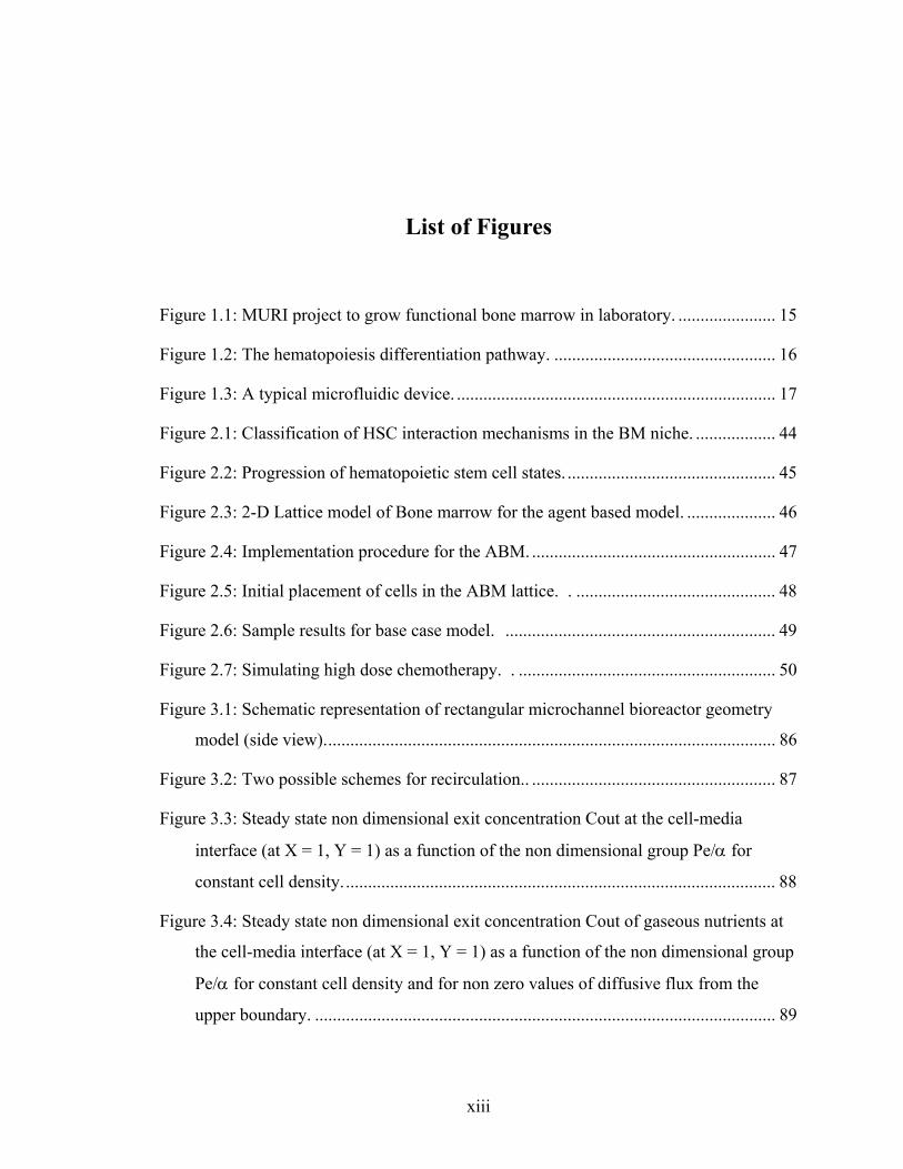
List of Figures .................................................................................................................. xiii
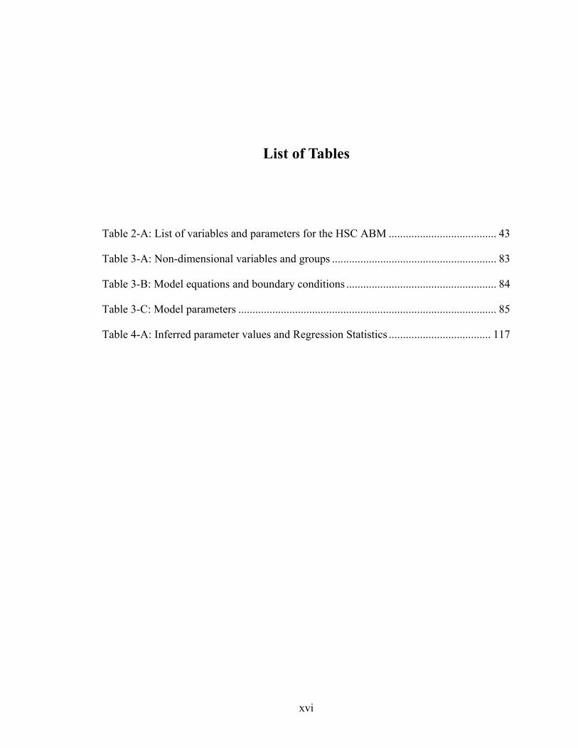
List of Tables ................................................................................................................... xvi
Abstract ........................................................................................................................... xvii
CHAPTER 1. Introduction ................................................................................................................... 1
1.1. Reaction-Diffusion Processes in Tissue Engineering & Quantitative Microscopy 1
1.2. Motivation ............................................................................................................... 4
1.3. Specific Aims .......................................................................................................... 5
1.4. Background ............................................................................................................. 7
1.4.1. Bone Marrow Biology ................................................................................ 8
1.4.2. Microfluidics based bioreactors for cell culture ......................................... 9
1.4.3. Quantitative Fluorescence Resonance Energy Transfer (FRET) imaging 11
1.5. Thesis Outline ....................................................................................................... 13
1.6. References ............................................................................................................. 18
2. Development of an Agent Based Model of Adult Hematopoietic Stem Cell
Interactions in Bone Marrow Niche ......................................................................... 21
Chapter Summary ......................................................................................................... 21
2.1. Introduction ........................................................................................................... 22

ix
2.2. Background and Previous Work ........................................................................... 24
2.2.1. HSC-Niche interactions in Bone Marrow ................................................. 24
2.2.2. Mathematical models of hematopoiesis process ....................................... 27
2.3. Formulating agent based model of HSC dynamics in the BM niche .................... 29
2.3.1. Progression of Hematopoietic Stem Cell States ....................................... 29
2.3.2. Preliminary differential equation model ................................................... 30
2.4. Agent based Model of HSC dynamics in the Niche ............................................. 32
2.4.1. Agents and Environment........................................................................... 32
2.4.2. Rules ......................................................................................................... 33
2.4.3. Implementation ......................................................................................... 39
2.4.4. Results and discussion .............................................................................. 40
2.5. Conclusions ........................................................................................................... 41
2.6. References ............................................................................................................. 51
3. Model-Based Analysis and Design of a Microchannel Reactor for Tissue
Engineering ................................................................................................................. 56
Chapter Summary ......................................................................................................... 56
3.1. Introduction ........................................................................................................... 57
3.2. Methods................................................................................................................. 60
3.2.1. Model Formulation ................................................................................... 60
3.2.2. Constitutive Relationships for uptake/secretion and cell proliferation rates
................................................................................................................... 65
3.2.3. Solution to model equations ...................................................................... 67
3.3. Results and discussion .......................................................................................... 70
3.3.1. Steady state model analysis at constant cell density: nutrient distribution 70

x
3.3.2. Steady state model analysis at constant cell density: Transport of cell-
secreted growth factors ............................................................................. 74
3.3.3. Steady state model analysis at constant cell density: Effect of media
recirculation .............................................................................................. 76
3.3.4. Unsteady state model analysis: Long term cell proliferation .................... 78
3.3.5. Effect of cell type heterogeneity ............................................................... 80
3.4. Conclusion ............................................................................................................ 82
3.5. References ............................................................................................................. 96
4. Quantitative Inference of Cellular Parameters from Microfluidic Cell Culture
Systems ........................................................................................................................ 99
Chapter Summary ......................................................................................................... 99
4.1. Introduction ......................................................................................................... 100
4.2. Methods............................................................................................................... 102
4.2.1. Experimental Methods ............................................................................ 102
4.2.2. Mathematical model formulation ............................................................ 104
4.2.3. Inferring parameter values from experimental data ................................ 108
4.2.4. Inferring confidence intervals for parameter values ............................... 110
4.3. Results and Discussion ....................................................................................... 111
4.3.1. Experimental measurements ................................................................... 111
4.3.2. Quantification of diffusion ...................................................................... 111
4.3.3. Quantification of cellular uptake rates for experimental cell densities ... 113
4.3.4. Quantification of cellular uptake rates for unified model of oxygen uptake
................................................................................................................. 114
4.4. Conclusion .......................................................................................................... 115
4.5. References ........................................................................................................... 123

xi
5. A computational approach to inferring cellular protein binding affinities from
quantitative FRET imaging ..................................................................................... 126
Chapter Summary ....................................................................................................... 126
5.1. Introduction ......................................................................................................... 127
5.2. Methods............................................................................................................... 130
5.2.1. Reaction System...................................................................................... 130
5.2.2. FRET Imaging Experiment ..................................................................... 131
5.2.3. 3D-FRET Stoichiometry Reconstruction for Improved Local
Concentration Estimates ......................................................................... 131
5.2.4. Computing Kd from image data ............................................................. 133
5.2.5. Generation of synthetic test data ............................................................. 135
5.2.6. Live cell FRET imaging.......................................................................... 136
5.3. Results and Discussion ....................................................................................... 138
5.3.1. Impact of Optical Blurring in estimating protein concentrations ........... 138
5.3.2. Inferring Kd from the image data ............................................................ 139
5.3.3. Using thresholds to counter optical distortion and noise ........................ 141
5.3.4. Inferring Kd in the presence of multiple protein binding states ............ 142
5.3.5. Inferring Kd when unlabelled proteins are present ................................. 143
5.3.6. Application to cellular data on Rac-PBD binding .................................. 144
5.4. Conclusion .......................................................................................................... 145
5.5. References ........................................................................................................... 158
6. Conclusions and Future Directions ......................................................................... 161
6.1. Summary of results ............................................................................................. 161
6.2. Future directions ................................................................................................. 163

xii
6.2.1. Theoretical investigations into cell-cell interactions and the role of niche
organization in adult stem cell systems .................................................. 163
6.2.2. Developing novel microfluidics-based devices for cell-based assays and
tissue engineering.................................................................................... 165
6.2.3. Inferring biophysical parameters for cellular reactions from imaging data ..
................................................................................................................. 167
6.3. Significance of current work ............................................................................... 169
6.4. References ........................................................................................................... 171
xiii
List of Figures
Figure 1.1: MURI project to grow functional bone marrow in laboratory. ...................... 15
Figure 1.2: The hematopoiesis differentiation pathway. .................................................. 16
Figure 1.3: A typical microfluidic device. ........................................................................ 17
Figure 2.1: Classification of HSC interaction mechanisms in the BM niche. .................. 44
Figure 2.2: Progression of hematopoietic stem cell states. ............................................... 45
Figure 2.3: 2-D Lattice model of Bone marrow for the agent based model. .................... 46
Figure 2.4: Implementation procedure for the ABM. ....................................................... 47
Figure 2.5: Initial placement of cells in the ABM lattice. . ............................................. 48
Figure 2.6: Sample results for base case model. ............................................................. 49
Figure 2.7: Simulating high dose chemotherapy. . .......................................................... 50
Figure 3.1: Schematic representation of rectangular microchannel bioreactor geometry
model (side view). ..................................................................................................... 86
Figure 3.2: Two possible schemes for recirculation.. ....................................................... 87
Figure 3.3: Steady state non dimensional exit concentration Cout at the cell-media
interface (at X = 1, Y = 1) as a function of the non dimensional group Pe/α for
constant cell density. ................................................................................................. 88
Figure 3.4: Steady state non dimensional exit concentration Cout of gaseous nutrients at
the cell-media interface (at X = 1, Y = 1) as a function of the non dimensional group
Pe/α for constant cell density and for non zero values of diffusive flux from the
upper boundary. ........................................................................................................ 89

xiv
Figure 3.5: The dimensionless outlet concentration Cout of the cell secreted autocrine
growth factor at the cell-media interface (at X = 1, Y = 1) as a function of the
operating variable group Pe/α for various values of ratio γ and Da. ........................ 90
Figure 3.6: The fraction of the cell secreted autocrine growth factor lost as a function of
the operating variable group Pe/α for various values of ratio γ and Da. .................. 91
Figure 3.7: Effect of recirculation ratio r on the dimensionless concentration (C) of the
autocrine growth (a) and nutrient concentration (b) along the dimensionless axial
distance (X) at the cell media interface (Y =1). ........................................................ 92
Figure 3.8: Optimization of the recirculation ratio for adequate growth factor retention
and nutrient availability inside the reactor. ............................................................... 93
Figure 3.9: Effect of nutrient gradients on the cell density distribution inside the
bioreactor. ................................................................................................................. 94
Figure 3.10: Effect of cell heterogeneity on the proliferation of cell co-culture of two cell
types, with doubling times of td1=16 and td2=32 hours and with dimensionless
bioreactor carrying capacity (Φ1 + Φ2)max= 10. ......................................................... 95
Figure 4.1: Microfabricated PDMS microreactor ........................................................... 118
Figure 4.2: Oxygen concentrations in the microdevice during culture of HepG2 cells. 119
Figure 4.3: Determination of the mass transfer coefficient kla from oxygen concentration
measurements and the model. ................................................................................. 120
Figure 4.4: Comparison of predicted and observed oxygen concentrations for oxygen
uptake model independent of cell density. ............................................................ 121
Figure 4.5: Model results with logistic growth factor densities for the proposed oxygen
uptake model. .......................................................................................................... 122
Figure 5.1: Point spread functions and synthetic test data. . ......................................... 148
Figure 5.2: Deconvolution is essential for quantitative measurement of protein
concentrations. ...................................................................................................... 149
Figure 5.3: Inferring Kd from wide-field image data: Effect of optical distortion. ........ 150

xv
Figure 5.4: Inferring Kd from confocal image data: Effect of optical distortion. ........... 151
Figure 5.5: The effect of detection noise on inference of Kd. ........................................ 152
Figure 5.6: Using thresholding to improve Kd inference. ............................................. 153
Figure 5.7: Inferring multiple values of Kd. .................................................................... 154
Figure 5.8 : Effect of partial labeling of interacting proteins. . ..................................... 155
Figure 5.9 : 3DFSR imaging of mammalian cells. ......................................................... 156
Figure 5.10 : Inferring Kd from 3DFSR images of mammalian cells.. ........................... 157
xvi
List of Tables
Table 2-A: List of variables and parameters for the HSC ABM ...................................... 43
Table 3-A: Non-dimensional variables and groups .......................................................... 83
Table 3-B: Model equations and boundary conditions ..................................................... 84
Table 3-C: Model parameters ........................................................................................... 85
Table 4-A: Inferred parameter values and Regression Statistics .................................... 117

xvii
Abstract
Computational Reaction-Diffusion Analysis of Cellular Systems for Tissue
Engineering and Quantitative Microscopy
by
Khamir H. Mehta
Chair: Jennifer J. Linderman
Reaction-diffusion mechanisms underlie communication of cells within and
among themselves and also with their environment. In this thesis, I have developed
computational approaches to better understand these mechanisms in the context of tissue
engineering and quantitative microscopy.
In the first part of my thesis I use an agent-based formalism to describe the
interactions of the hematopoietic stem cells in the bone marrow niche and their role in
hematopoiesis. Using a mathematical representation of the interactions, I create a
framework that can be used to question the role and relative importance of cellular
interactions inside the niche in the context of hematopoiesis. In the second part, I apply
deterministic models to identify general principles for design and operation of

xviii
microfluidics-based perfusion bioreactors for cell cultures. I use model-based analysis to
arrive at optimal strategies for designing bioreactor geometry, media perfusion and
recirculation, initial cell seeding composition for co-cultures, and retaining cell-secreted
autocrine factors. I further demonstrate the utility of these models to infer the cellular
properties from data on experimental measurements by inferring oxygen uptake
parameters of HepG2 (human hepatocellular carcinoma) cells. In the final part of my
thesis, I turn my attention to the reaction systems inside the cell and present
computational algorithms to infer the local protein binding dissociation constant (Kd)
from 3-dimensional Fluorescence Resonance Energy Transfer (FRET) microscopy data
on live cells. I analyze the performance of the algorithm using synthetic test data, both in
the absence and presence of endogenous (unlabeled) proteins, and show that
deconvolution is essential for quantitative inference of local Kd, I test the algorithm to
quantify the interaction between YFP (yellow fluorescent protein)-Rac and CFP (cyan
fluorescent protein)-PBD in mammalian cells.
Taken together, the results offer novel insights into model-based design of in vitro
biological systems for target applications in tissue engineering, microfluidic bioanalytical
devices and quantitative microscopy and also present new approaches for quantitative
inference from the associated experimental data.

1
Chapter 1
1.Introduction
1.1. Reaction-Diffusion Processes in Tissue Engineering & Quantitative
Microscopy
Complex networks of reactions occurring at various scales form the fundamental
machinery by which any living organism can perform essential functions to maintain and
propagate itself. For example, the process of metabolism is but a series of chemical
reactions which result in breakdown of large complex molecules resulting in the
generation of energy or making building blocks for cellular function. Similarly, the
biological signaling transduction occurs via series of reactions occurring within/among
cells by which the cells can respond to the changes in the environment. The
understanding of biological reaction networks, therefore, occupies a significant position
in the area of biological engineering, and many efforts have been made to get a better
understanding of cellular metabolic and signaling networks both from an experimental as
well as modeling standpoint (e.g Crampin, et al. 2004 ; Kholodenko 2006 ;

2
Mullassery, et al. 2008a ; Papin, et al. 2005 ; Rangamani and Iyengar 2008 ; Ross 2008 ;
Wolkenhauer, et al. 2005 ). Further, the effect of spatial arrangement and diffusion in
such systems is also a subject of active research, and the role of spatial dimensional and
diffusion is shown to be important for signaling systems (Brinkerhoff and Linderman
2005 ; Brinkerhoff, et al. 2008 ).
As in usual chemical systems, the characterization of the equilibrium and dynamic
reaction parameters remain crucial to the success of any modeling approach for
biochemical reaction networks. Along with the usual methods of determination of
reaction parameters, quantitative fluorescent microscopy imaging of live cells offers the
promise to measure the reaction parameters in its native environment and hence is the
center of attention of various research groups (Benninger, et al. 2008 ; Day and Schaufele
2008 ; Kherlopian, et al. 2008 ; Mullassery, et al. 2008b ). Among them, visualization of
protein-protein binding by Fluorescence resonance energy transfer (FRET) is a effective
way to gather data on cellular protein reactions (Chen, et al. 2007 ; Hoppe 2003 ; Hoppe
2007 ; Kenworthy 2001 ; Lippincott-Schwartz, et al. 2001 ; You, et al. 2006 ). However,
the process of inferring information about cellular reactions from the imaging data is far
from understood.
Recently, there has been a focus on developing in vitro systems that can mimic
the native cellular conditions. Such systems can be of vital importance, as they can offer
the possibility of probing the cells to characterize their behavior under controlled
environmental conditions and also quantitatively measure the associated responses. From
a medical perspective, they can be used to grow functional tissues that can be further used
for transplantation. This research area, termed ‘tissue engineering’, aims at developing

3
replacement organs in a laboratory (in vitro organs) starting from a small population of
donor cells and providing them with appropriate microenvironment for development of
target tissues (Langer and Vacanti 1993 ; Vacanti and Langer 1999 ). The development of
such tissue engineering methods will involve extensive experimentation for screening,
optimization, and implementation of the final tissue. Considering that most of these
systems have an underlying reaction-diffusion mechanism, mathematical analysis and
predictive models can play a crucial role in reducing the expensive experimentation and
successful application of tissue engineered therapy.
In particular, the development of in vitro culture systems to maintain and expand
stem cells (both, adult as well as embryonic) has great therapeutic potential, considering
that, in principle, the stem cells are mulipotent and can be made to proliferate and
differentiate into almost any tissue. Research efforts in engineering stem cells for
developing functional tissues like bone and blood have been fairly successful and well
understood (Mauney, et al. 2005 ; Mukhopadhyay, et al. 2004 ; Zandstra and Nagy 2001).
However, optimal strategies to maintain and expand stem cells still remain elusive.
Microfabricated perfusion based bioreactors have emerged as strong candidates for
developing in vitro cell culture systems for both tissue engineering as well as developing
new platforms to be used as biosensors (Ainslie and Desai 2008 ; Andersson and van den
Berg 2004 ; Khademhosseini, et al. 2006 ; Park and Shuler 2003a ). Compared to
traditional static cell culture methods, the media for such new bioreactors is continuously
perfused, to provide a dynamically controlled microenvironment for the cells in the
culture. Considering the basic mechanisms involved in the growth and culture of cells in
such bioreactors would be based on diffusional and convective transport coupled with the

4
reactive uptake/secretion, a mathematical analysis of these systems can help with
improving the design without expensive experimentation.
1.2. Motivation
The initial work for this thesis was a part of modeling support for the
multidisciplinary university research initiative (MURI) project aimed at growing
functional bone marrow in laboratory. The bony organ was envisaged to have
mineralized tissue, marrow and microcirculatory compartments, and can be useful for
variety of potential applications including tissue-replacement therapy and also for use as
novel and life-saving biosensors. It was proposed to use the multipotent stem cells
isolated from the adult bone marrow, provide them with appropriate environment (e.g.
growth factors, nutrients etc), and have them form the bony organ in a microfluidics
based bioreactor. It was hypothesized that it is possible to recreate the various
components of the bone from the mesenchymal and hematopoietic stem cells of bone
marrow, by providing the required environment at appropriate location and time in the
bioreactor. It was proposed to use mesenchymal stem cells (MSCs) to form mineralized
tissue and marrow stroma, and hematopoietic stems cells (HSCs) will be introduced into
this engineered bone tissue to form the blood tissue by establishing hematopoiesis, or the
process of blood formation. Figure 1.1 shows the schematic diagram of the overall
project strategy, and how this work was expected to fit in.
The cell behavior is governed by the microenvironment within which it resides.
The environment in turn is regulated by the collection of cells residing in it through a

5
complex network of paracrine and autocrine soluble signals as well as cell-cell and cell-
ECM signaling mediated by reactions and transport of signals to the cell surface. Further
physicochemical parameters such as pH, temperature, nutrient concentration and
mechanical stimuli etc also seem to affect the cell phenotype (Khademhosseini &
Zandstra, 2002). Species transport models to predict the spatial distribution of such
factors along with soluble signaling molecules like bone morphogenetic proteins,
ascorbic acid, dexamethasone etc inside the bioreactor, hence can be especially useful to
obtain a defined and controllable microenvironment which can support the stem cell
differentiation into the desired phenotype. The models should incorporate the effect of
cellular uptake and secretion rates, most of which are non-linearly related to the
distribution and state of the cells and associated signaling molecules.
The specific aims of my thesis were hence motivated in part, by the MURI
project, and involved building computational models for better understanding the
hematopoietic stem cell systems, design and optimization of growth and culture of cells
in microfabricated bioreactors, and using the experimental data therein to infer and
characterize the reaction parameters in these systems.
1.3. Specific Aims
The preliminary objective of my research was to construct quantitative models of
cell behavior as a function of microenvironmental variables, for the particular case of
hematopoietic bone marrow cells, and help in design of the microfabricated device to

6
grow the aforementioned functionalized bone marrow tissue. An associated objective of
modeling was to develop an inference strategy that can take the measurements from such
experiments as input, and characterize the biophysical parameters of the cells as an
output.
It was further seen that understanding the native interactions and regulatory
mechanisms governing the hematopoietic stem cells inside the bone marrow is a key
component to developing successful methods for maintenance and ex vivo expansion of
the hematopoietic stem cells. My thesis work, hence, also included the theoretical
analysis of interactions and regulatory mechanisms governing hematopoiesis inside the
bone marrow. Finally, as mentioned earlier, the behavior of stem cells is governed by
reactions and interactions at internal levels as well. While little is known definitively
about the molecular control of hematopoiesis, it was envisaged that the future
developments, especially in the field of fluorescent imaging can help us identify the
important protein-protein interactions forming the molecular basis of hematopoiesis.
Quantification of such interactions hence can aid in developing further analysis tools
which are useful for developing a successful strategy to realize the therapeutic potential
of the hematopoietic stem cells. In this context, as a first step, my thesis focuses on
inferring equilibrium binding of proteins in live cells from three dimensional FRET
imaging experiments.
In this thesis I have explored the application of computational modeling with the
following specific aims.

7
1. Develop a theoretical and computational framework to analyze the relative
importance of various known interactions regulating the differentiation and self
renewal of hematopoietic stem cells inside the bone marrow niche.
2. Develop mathematical models of transport of nutrients and soluble growth factors
and its effect on the growth of cell cultures in a microfluidics based bioreactor
systems. Using these models, analyze, and prescribe the optimal design and
operational strategies to culture given cell type(s) with target specifications.
3. Develop a methodology to quantitatively infer the biophysical parameters from
experimental measurements from microfluidics based cell cultures. Demonstrate
its applicability by inferring the oxygen uptake rate of cell cultures from the
measurement of oxygen concentrations.
4. Develop and validate computational strategy to infer reaction parameters from
quantitative FRET imaging.
1.4. Background
In this thesis I investigate the application of computational modeling in three
areas: 1) Modeling hematopoietic interactions in bone marrow, 2) Modeling and analysis
of microfluidics based perfusion bioreactors and 3) Analysis of FRET imaging data for
inferring protein binding in live cells. I present below a brief background and previous
modeling work on each of these areas, details of which can be found in the subsequent
chapters wherein details of my work is also presented.

8
1.4.1. Bone Marrow Biology
The bone marrow consists primarily of two kinds of cell types a) the
hematopoietic cells associated with blood cells and b) bone marrow stromal cells
(BMSCs) related to the marrow stroma. The bone marrow forms the principal site for
hematopoiesis: the process of formation of blood cells from the progenitor cells. The
bone marrow produces approximately 2.5 billion erythrocytes (red blood cells), 2.5
billion platelets, and 1 billion white cells per kilogram of body weight each day
(Mantalaris, et al, 1998), which clearly indicates high level of activity of the
hematopoietic cells. The terminally differentiated blood cells are incapable of
proliferation, and the replacement of these cell types is accomplished by differentiation
and proliferation of single pluripotent cell type called the Hematopoietic stem cell (HSC)
through the process of hematopoiesis. The hematopoiesis process is a subject of extensive
research, and the multiple hierarchical steps through which the HSC goes through to give
rise to terminally differentiated cells is known. Figure 1.2 outlines the hematopoiesis
differentiation pathway for HSC.
The marrow stromal cells and their secretions in the form of extracellular matrices
(ECMs) form the microenvironment (niche) within which the hematopoietic cells reside,
proliferate and differentiate. The complex interplay between the hematopoietic cells, the
stromal cells and the ECM regulate the process of hematopoiesis through various
signaling molecules, cell-cell and cell-ECM interactions (Calvi et al, 2003, Attar &
Scadden, 2004). Traditional culture techniques however cannot provide the appropriate
environment to support and differentiate the hematopoietic progenitors and hence the
idea of cultivating the hematopoietic cells along with the stromal cells was suggested by

9
Dexter in late 1970s. It was hypothesized that the stromal cells would provide the
appropriate growth and signaling molecules for the hematopoietic cells survival. The first
stromal cell mediated long-term bone marrow cultures were developed for the murine
system by Dexter and co-workers, and is referred to as Dexter cultures. Further
refinement of cell cultures used the knowledge of cell biology and the availability of
various cytokines known to promote growth and differentiation of hematopoietic cells
(Cabrita et al, 2003). The most important drawback in most systems is the lack of long
term culture maintenance and multi-lineage differentiation which can be associated with
the lack of maintenance of undifferentiated stem cells. The identification of culture
conditions and bioreactor system design which can achieve HSC expansion hence,
remains one of the major research topics of experimental hematology. I intend to
contribute to this area by developing a modeling framework to better understand the
interactions and mechanisms behind the functioning of hematopoietic stem cells in the
bone marrow.
1.4.2. Microfluidics based bioreactors for cell culture
Traditional static cell culture systems cannot provide the three dimensional
microenvironment with and all the interactions for cells as their native sites, and hence it
is often thought that they alter the cellular properties, especially those related to growth
and differentiation. Alternatively, the newly developed microfluidics based cell culture
methods can offer controlled supply of media, buffers, and also real time analysis by
integration with analytical techniques including imaging. Recent advances in
microfabrication technology also can now allow us to create an microenvironment which

10
is very similar to in vivo (Li, et al. 2003 ; Paguirigan and Beebe 2008 ; Park and Shuler
2003 ; Weibel, et al. 2005 ).
Typically such devices consist of a microfabricated device where micron size cell
culture channels are etched out of a chip with a suitable substrate. Poly(dimethylsiloxane)
(PDMS) forms a favored substrate for most cell culture applications owing to its
biocompatibility, the ease of fabrication, and also due to its high gas permeability. Figure
1.3 shows a typical picture of PDMS fabricated microfluidic device. The media flow in
such devices is controlled by either standard peristaltic or syringe pumps, or with
sophisticated techniques like Braille displays (Gu, et al. 2004 ).
Micofabricated bioreactor chips are integrated with microfluidics based perfusion
systems, and have been reported for various applications involving the measurement of
cellular responses to changes in the environment and tissue engineering (Ainslie and
Desai 2008 ; Baudoin, et al. 2007 ; Park and Shuler 2003b ; Yang, et al. 2008 ). While the
ability to provide temporally and spatially varying environment for the cell culture offers
a large experimental design space, it also makes the job of optimizing the experimental
conditions more difficult and time consuming. Therefore, there have been a lot of efforts
in computational modeling, especially in the reaction/diffusion, transport and cell growth
processes associated with the growth of cells in the artificial support materials (scaffolds)
or in bioreactors (Hutmacher and Singh 2008 ; Nichols and Cortiella 2008 ; Pancrazio, et
al. 2007 ; Semple, et al. 2005 ; Sengers, et al. 2007 ). These efforts have been able to
contribute in developing and optimization functional tissues like liver, cartilage, etc
(Chung and Burdick 2008 ; Fiegel, et al. 2008 ; Pryor and Vacanti 2008 ; Schoenfeld, et
al. 2007 ). However, a using the model to identify design guidelines for developing new

11
bioreactors and their operational strategy, as with usual chemical reactor systems is not
yet studied. I intend to bridge this gap with my research in this thesis.
1.4.3. Quantitative Fluorescence Resonance Energy Transfer (FRET) imaging
The introduction of green fluorescent proteins and its variants have opened up
new and exciting avenues in fluorescent microscopy imaging. The FRET process is a
distance-dependent physical process by which energy is transferred non-radiatively from
an excited molecular fluorophore (the donor) to another fluorophore (the acceptor)
(Lakowicz 1999 ). FRET microscopy can measure the proximity of two previously
tagged fluorescent biomolecules inside live cells, and hence give a measure of their
interaction. The amount of energy transfer of mostly depends on the distance between the
two fluorophores (~ d-6) and the spectral properties of the two fluorophores. Quantitative
measurement of energy transfer in FRET entails the estimation of the efficiency of
energy transfer, also known as the FRET efficiency.
A typical intensity based FRET experiment would involve the imaging of cell at
two wavelengths corresponds to the donor and acceptor fluorophores. If there are real
interactions of the two molecules with which the fluorophores are attached, an increase in
acceptor emission is seen along with a decreased donor emission. If we know the fret
efficiency, we can estimate the relative amounts of the donor, acceptor and the donor
acceptor complex respectively. There are excellent reviews describing the applicability
and experimental features of FRET microscopy, and recent advances have enabled
considerable degree of quantification. (Berney and Danuser 2003 ; Garini, et al. 2006 ;
Gordon, et al. 1998 ; Hoppe, et al. 2002 ; Hoppe 2007 ; Sekar and Periasamy 2003).
12
Currently FRET experiments are mostly qualitative and the data are in the form of
complex data sets with large numbers of images of a single cell, highlighting the need for
data analysis and abstraction. Such imaging information can be potentially used to
determine various biophysical parameters. In particular steady state measurements of
protein concentration distributions might be used to determine the apparent protein
disassociation constant (Kd) for a protein pair which can be further used in reconstruction
of cellular signaling networks. Recent developments in quantitative fluorescence
microscopy techniques have allowed the measurement of the local concentration of
proteins genetically altered for fluorescent activity (Wu and Pollard, 2005). There have
also been efforts to employ the quantitative understanding of FRET to estimate the
relative concentrations of donor and acceptor molecules (Chen et al., 2006, Thaler et al.,
2005, Hoppe et al., 2002).
A key problem associated with quantifying these FRET measurements via
microscopy is blurring. Any microscope imaging an object suffers from optical image
blurring associated with the light from out-of focus planes as characterized by the point
spread function (PSF) of the microscope. This blurring limits the use of the intensity-
concentration correlation for dissimilar objects and can compromise the local nature of
information of protein interactions by spatially averaging the intensity. The direct use of
images after spectral overlap correction to estimate the local concentrations of the
molecules through calibration hence can be erroneous. The inaccuracy in the estimate
would be severe for a ‘more diffused’ PSF, where the intensity of the unit pixel is more
spread out spatially. Efforts have been made to reduce the optical blurring at the
instrument level and hence preserve the local information. Confocal microscopes

13
minimize such blurring by having a ‘less diffused’ PSF compared to the conventional
wide-field microscopes. It has been also proposed to use efficient image-deconvolution
algorithms to increase the local accuracy of the images, making it possible to estimate the
local protein concentrations with less error (Hoppe et al, 2006). Deconvolution or image
reconstruction involves using information on the instrument PSF to estimate the intensity
of the original object voxel and thereby calculate the actual number of molecules in it.
While it is understood that spatial blurring will affect the inference of biophysical
parameters from images via the calibration, a systematic study of its impact and the
extent to which deconvolution can alleviate the problem is still unavailable. In this thesis,
I contribute to this are by investigating the feasibility of inferring equilibrium binding
affinity from image data using a computational algorithm.
1.5. Thesis Outline
In this thesis, I present the results of my research as per the specific aims outlined
in the section 1.3.
In Chapter 2, I describe the development of a computational model describing the
self-renewal and differentiation of adult hematopoietic stem cell inside an bone marrow
niche. I also present the results of this first generation model, in context of the
hematopoiesis process.
Chapter 3 and 4 deal with the computational model and its applications in design
and inference from microfluidic cultures respectively. Specifically, in chapter 3, I
describe the development of a partial differential equation model of nutrient and soluble

14
growth factor transport inside a microfabricated bioreactor, and apply it for prescribing
optimal design and operating conditions. In chapter 4, I apply the inverse form of the
model to infer the oxygen uptake rates of cell culture from experimental data on oxygen
uptake rates.
In Chapter 5 I present an algorithm to infer the protein binding affinities from a
intensity based FRET experimental data. I demonstrate the applicability of my algorithm
by using a synthetic, in-silico system as well as binding of Rac-PBD in mammalian cells.
Finally, I present my overall conclusions and future directions in chapter 6.

15
Figure 1.1: MURI project to grow functional bone marrow in laboratory. The HSCs and MSCs will be isolated using flow cytometry (FACS), and a bone tissue will be grown in a dynamic bioreactor device using polymeric scaffolds to encapsulate the MSCs and introducing HSCs in the bioreactor. The research described in this thesis was associated with creating mathematical models for design and optimization of culture conditions in the microfabricated device, the site of growth and development of bone marrow tissue.
FACS

16
Figure 1.2: The hematopoiesis differentiation pathway. The pluripotent HSC is believed to be of two types: Long term culture initiating cell with unlimited self-renewal, and short-term with limited self renewal capacity. (Reproduced from http://www.bloodlines.stemcells.com/img/Metcalf_Fig3_2.gif ).

17
Figure 1.3: A typical microfluidic device. A typical microfluidic device etched in PDMS is shown on the top. The channels are highlighted by green food dye. A schematic of the channel organization and the Braille pumps along with valves is shown below. (Reproduced from G Mehta, PhD Thesis, 2008)

18
1.6. References
Ainslie KM, Desai TA. 2008. Microfabricated implants for applications in therapeutic delivery, tissue engineering, and biosensing. Lab Chip 8:1864-1878.
Andersson H, van den Berg A. 2004. Microfabrication and microfluidics for tissue engineering: state of the art and future opportunities. Lab Chip 4:98-103.
Attar EC, Scadden DT. 2004. Regulation of hematopoietic stem cell growth. Leukemia 18:1760-1768.
Baudoin R, Corlu A, Griscom L, Legallais C, Leclerc E. 2007. Trends in the development of microfluidic cell biochips for in vitro hepatotoxicity. Toxicol In Vitro 21:535-544.
Benninger RK, Hao M, Piston DW. 2008. Multi-photon excitation imaging of dynamic processes in living cells and tissues. Rev Physiol Biochem Pharmacol 160:71-92.
Berney C, Danuser G. 2003. FRET or no FRET: a quantitative comparison. Biophys J 84:3992-4010.
Brinkerhoff CJ, Choi JS, Linderman JJ. 2008. Diffusion-limited reactions in G-protein activation: unexpected consequences of antagonist and agonist competition. J Theor Biol 251:561-569.
Brinkerhoff CJ, Linderman JJ. 2005. Integrin dimerization and ligand organization: key components in integrin clustering for cell adhesion. Tissue Eng 11:865-876.
Calvi LM, Adams GB, Weibrecht KW, Weber JM, Olson DP, Knight MC, Martin RP, Schipani E, Divieti P, Bringhurst FR, Milner LA, Kronenberg HM, Scadden DT. 2003. Osteoblastic cells regulate the haematopoietic stem cell niche. Nature 425:841-846.
Chen H, Puhl HL,3rd, Ikeda SR. 2007. Estimating protein-protein interaction affinity in living cells using quantitative Forster resonance energy transfer measurements. J Biomed Opt 12:054011.
Chung C, Burdick JA. 2008. Engineering cartilage tissue. Adv Drug Deliv Rev 60:243-262.
Crampin EJ, Schnell S, McSharry PE. 2004. Mathematical and computational techniques to deduce complex biochemical reaction mechanisms. Prog Biophys Mol Biol 86:77-112.
Day RN, Schaufele F. 2008. Fluorescent protein tools for studying protein dynamics in living cells: a review. J Biomed Opt 13:031202.
Fiegel HC, Kaufmann PM, Bruns H, Kluth D, Horch RE, Vacanti JP, Kneser U. 2008. Hepatic tissue engineering: from transplantation to customized cell-based liver directed therapies from the laboratory. J Cell Mol Med 12:56-66.
Garini Y, Young IT, McNamara G. 2006. Spectral imaging: principles and applications. Cytometry A 69:735-47.

19
Gordon GW, Berry G, Liang XH, Levine B, Herman B. 1998. Quantitative fluorescence resonance energy transfer measurements using fluorescence microscopy. Biophys J 74:2702-13.
Gu W, Zhu X, Futai N, Cho BS, Takayama S. 2004. Computerized microfluidic cell culture using elastomeric channels and Braille displays. Proc Natl Acad Sci U S A 101:15861-15866.
Hoppe A, Christensen K, Swanson JA. 2002. Fluorescence resonance energy transfer-based stoichiometry in living cells. Biophys J 83:3652-64.
Hoppe A. 2007. Quantitative FRET Microscopy of Live Cells. Imaging Cellular and Molecular Biological Functions. p 157-181.
Hoppe AD. 2003. Development of quantitative FRET microscopy for study of RHO GTPase and Phosphoninositide signaling in phagocytosis. 116 -118.
Hutmacher DW, Singh H. 2008. Computational fluid dynamics for improved bioreactor design and 3D culture. Trends Biotechnol 26:166-172.
Kenworthy AK. 2001. Imaging protein-protein interactions using fluorescence resonance energy transfer microscopy. Methods 24:289-96.
Khademhosseini A, Bettinger C, Karp JM, Yeh J, Ling Y, Borenstein J, Fukuda J, Langer R. 2006. Interplay of biomaterials and micro-scale technologies for advancing biomedical applications. J Biomater Sci Polym Ed 17:1221-1240.
Kherlopian AR, Song T, Duan Q, Neimark MA, Po MJ, Gohagan JK, Laine AF. 2008. A review of imaging techniques for systems biology. BMC Syst Biol 2:74.
Kholodenko BN. 2006. Cell-signalling dynamics in time and space. Nat Rev Mol Cell Biol 7:165-176.
Lakowicz J. 1999. Principles of Fluorescence Spectroscopy. New York:Plenum.
Langer R, Vacanti JP. 1993. Tissue engineering. Science 260:920-926.
Li N, Tourovskaia A, Folch A. 2003. Biology on a chip: microfabrication for studying the behavior of cultured cells. Crit Rev Biomed Eng 31:423-488.
Lippincott-Schwartz J, Snapp E, Kenworthy A. 2001. Studying protein dynamics in living cells. Nat Rev Mol Cell Biol 2:444-56.
Mantalaris A, Keng P, Bourne P, Chang AY, Wu JH. 1998. Engineering a human bone marrow model: a case study on ex vivo erythropoiesis. Biotechnol Prog 14:126-133.
Mauney JR, Volloch V, Kaplan DL. 2005. Role of adult mesenchymal stem cells in bone tissue engineering applications: current status and future prospects. Tissue Eng 11:787-802.
Mukhopadhyay A, Madhusudhan T, Kumar R. 2004. Hematopoietic stem cells: clinical requirements and developments in ex-vivo culture. Adv Biochem Eng Biotechnol 86:215-253.
Mullassery D, Horton CA, Wood CD, White MR. 2008a. Single live-cell imaging for systems biology. Essays Biochem 45:121-133.

20
Nichols JE, Cortiella J. 2008. Engineering of a complex organ: progress toward development of a tissue-engineered lung. Proc Am Thorac Soc 5:723-730.
Paguirigan AL, Beebe DJ. 2008. Microfluidics meet cell biology: bridging the gap by validation and application of microscale techniques for cell biological assays. Bioessays 30:811-821.
Pancrazio JJ, Wang F, Kelley CA. 2007. Enabling tools for tissue engineering. Biosens Bioelectron 22:2803-2811.
Papin JA, Hunter T, Palsson BO, Subramaniam S. 2005. Reconstruction of cellular signalling networks and analysis of their properties. Nat Rev Mol Cell Biol 6:99-111.
Park TH, Shuler ML. 2003. Integration of cell culture and microfabrication technology. Biotechnol Prog 19:243-253.
Pryor HI,2nd, Vacanti JP. 2008. The promise of artificial liver replacement. Front Biosci 13:2140-2159.
Rangamani P, Iyengar R. 2008. Modelling cellular signalling systems. Essays Biochem 45:83-94.
Ross J. 2008. From the determination of complex reaction mechanisms to systems biology. Annu Rev Biochem 77:479-494.
Schoenfeld AJ, Landis WJ, Kay DB. 2007. Tissue-engineered meniscal constructs. Am J Orthop 36:614-620.
Sekar RB, Periasamy A. 2003. Fluorescence resonance energy transfer (FRET) microscopy imaging of live cell protein localizations. J Cell Biol 160:629-633.
Semple JL, Woolridge N, Lumsden CJ. 2005. In vitro, in vivo, in silico: computational systems in tissue engineering and regenerative medicine. Tissue Eng 11:341-356.
Sengers BG, Taylor M, Please CP, Oreffo RO. 2007. Computational modelling of cell spreading and tissue regeneration in porous scaffolds. Biomaterials 28:1926-1940.
Vacanti JP, Langer R. 1999. Tissue engineering: the design and fabrication of living replacement devices for surgical reconstruction and transplantation. Lancet 354 Suppl 1:SI32-4.
Weibel DB, Garstecki P, Whitesides GM. 2005. Combining microscience and neurobiology. Curr Opin Neurobiol 15:560-567.
Wolkenhauer O, Ullah M, Wellstead P, Cho KH. 2005. The dynamic systems approach to control and regulation of intracellular networks. FEBS Lett 579:1846-1853.
Yang ST, Zhang X, Wen Y. 2008. Microbioreactors for high-throughput cytotoxicity assays. Curr Opin Drug Discov Devel 11:111-127.
You X, Nguyen AW, Jabaiah A, Sheff MA, Thorn KS, Daugherty PS. 2006. Intracellular protein interaction mapping with FRET hybrids. Proc Natl Acad Sci U S A 103:18458-63.
Zandstra PW, Nagy A. 2001. Stem cell bioengineering. Annu Rev Biomed Eng 3:275-305.

21
Chapter 2
2.Development of an Agent Based Model of Adult
Hematopoietic Stem Cell Interactions in Bone Marrow Niche
Chapter Summary
Realization of the vast therapeutic potential of adult hematopoietic stem cells
requires technologies and strategies for in vitro maintenance and expansion of
hematopoietic stem cells in cell cultures and remains an outstanding challenge. The
development of successful stem cell expansion protocols can greatly be aided by
understanding the fundamental interactions of these cells in their native niches. In
particular, in this chapter I investigate the role of various known interaction types in
regulating adult hematopoietic stem cell (HSC) maintenance and proliferation in bone
marrow niches using a computational model. I present the modeling framework to
handle experimental observations with varying degree of quantification and its

22
implementation. The multi-agent based computational model is built using the
experimental observations of HSC-niche interactions, and it simulates the regulation of
activation, self renewal and differentiation of HSCs via cell-cell, cell-local
microenvironment and cell-systemic environment interactions. I also present the results
of the model in response to hypothetical experiments simulating
pathological/experimental conditions. My results are significant in developing a
comprehensive computational model to investigate critical regulatory mechanisms
governing the stem cell behavior.
2.1. Introduction
Adult stem cell systems offer a relatively easy procurable alternative to using
embryonic stem cell for next generation cell based therapy (Gordon 2008 ; Kuehnle and
Goodell 2002 ; Nagy, et al. 2005 ; Rafii and Lyden 2003 ; Tataria, et al. 2006 ). In
particular the clinical applications of the adult hematopoietic stem cell have generated
enormous interest both in the medical as well as science community (Burt, et al. 2008 ;
Chan and Yoder 2004 ; Devine, et al. 2003 ; Tateno, et al. 2006 ).
The hematopoietic stem cell is by far the most researched of the adult stem cells
(Chan and Yoder 2004 ; Huang, et al. 2007 ; Murray, et al. 1994 ; Orlic, et al. 1994 ;
Ratajczak 2008 ). The bone marrow (BM) forms the principal source of adult
hematopoietic stem cells and is the primary site for hematopoiesis, producing
approximately 2.5 billion erythrocytes (red blood cells), 2.5 billion platelets, and 1 billion
white cells per kilogram of body weight each day (Mantalaris, et al. 1998). The

23
terminally differentiated blood cells are incapable of proliferation, and the replacement of
these cell types is accomplished by differentiation and proliferation of a single pluripotent
cell type, the hematopoietic stem cell (HSC), through the process of hematopoiesis.
HSCs have the capability for both long term and short term self renewal and differentiate
into other blood cell types (figure 1.2) and are very few in number (< 0.001% of BM
cells) in the bone marrow (Wilson, et al. 2007 ). While BM remains the primary site of
adult HSC residence they are also known to migrate to other sites ( marrow regions of
other bones) BM sites via the peripheral blood flow, and hence HSCs can also be
harvested from circulating blood flow in adults.
BM is also home to various other cell types, including mesenchymal stem cells
and associated stromal cells. These cells and their secretions in the form of extracellular
matrices (ECMs) form the microenvironment (niche) within which the hematopoietic
cells reside, proliferate and differentiate. BM hence is a important site for hematopoiesis.
The complex interplay between the hematopoietic cells, the stromal cells and the ECM
regulate the process of hematopoiesis through various signaling molecules, cell-cell and
cell-ECM interactions (Calvi, et al. 2003, Attar & Scadden, 2004) and by systemic
secretion of stimulatory hormones. In other words, the self renewal, differentiation and
proliferation of the hematopoietic progenitors are tightly regulated by the stem cell niche
(Kopp, et al. 2005 ; Spradling, et al. 2001 ; Suda, et al. 2005a ; Suda, et al. 2005b ;
Taichman 2005 ; Wilson and Trumpp 2006 ; Yin and Li 2006 ; Zhu and Emerson 2004 ).
Understanding the behavior of HSC in its native microenvironment (niche) of the bone
marrow is of fundamental interest to biologists as well as for applied biomedical
engineers, as it can give vital information about the microenvironment required for

24
maintenance and expansion of HSC in vitro. The role of niche is hence the center of
multitude of research efforts, and many important features of HSC-niche interactions
have been unraveled (Arai, et al. 2005b ; Arai and Suda 2007 ; Crocker, et al. 1988 ; Kiel,
et al. 2005 ; Wilson, et al. 2007 ). However, a complete understanding of the relative
importance of these interactions and the role of niche still remains a point of speculation.
Furthermore, experimental investigation of individual interactions remains a difficult and
time consuming task, considering that it is seldom possible to study the interaction in
isolation or at controlled level. Mathematical models of these systems can help
understand the various mechanisms behind the HSC regulation, and can also reduce
experimentation for effective hypothesis testing.
2.2. Background and Previous Work
2.2.1. HSC-Niche interactions in Bone Marrow
The concept of niches and their role is still evolving (Adams and Scadden 2006 ;
Adams 2008 ; Arai, et al. 2005a ; Frisch, et al. 2008 ; Kiel and Morrison 2006 ; Kiel and
Morrison 2008 ; Kopp, et al. 2005 ; Li and Li 2006 ; Martinez-Agosto, et al. 2007 ;
Moore 2004 ; Moore and Lemischka 2006 ; Morrison and Spradling 2008 ; Porter and
Calvi 2008 ; Raaijmakers and Scadden 2008 ). However, it is generally accepted that the
two primary types of niche supporting the HSC are the osteoblastic niche and the
vascular niche (Suda, et al. 2005a ; Wilson, et al. 2007 ). It is further understood that the
HSC remains in a predominantly a quiescent state and is periodically activated to give
rise to the activated cell, which undergoes further changes (self renewal, differentiation,

25
migration) to give rise to a stable pool of committed progenitors which are the source of
blood cells via the process of rapid proliferation and differentiation.
The exact set of mechanisms and interactions of the cells inside the niche remain
a subject of speculation; however, a study of known pathways and interactions governing
hematopoiesis can help us systematically categorize the interaction into subsets enabling
easier comprehension. For the purpose of this research, I have classified the interactions
into three broad categories.
The first kind of interaction constitutes the direct adhesion of cells to HSCs and
is referred to as direct cell-cell interaction in this work. Regulatory mechanisms
involving special osteoblasts, the spindle-shaped N-cadherin+CD45– osteoblastic (SNO)
cells in the BM niche, are of this kind. For example, it is shown that stromal cells like
osteoblasts, or the CXC chemokine ligand 12 (CXCL12) expressing reticular cells, are
important regulatory components of the HSC supportive niche which act via direct cell
adhesion receptors (Calvi, et al. 2003 ; Calvi 2006 ; Stier, et al. 2005 ; Sugiyama, et al.
2006 ; Taichman 2005 ; Zhang, et al. 2003 ; Zhu and Emerson 2004 ). Macrophages can
also interact with hematopoietic cells via cell surface adhesion receptors (Conrad and
Emerson 1998 ). The exact mechanisms by which the cellular adhesion regulates the HSC
state, and hence hematopoiesis is still a matter of speculation; it is conceivable that the
the bound adhesion receptor could trigger further intracellular pathways, or the regulation
could be via simple mechanical support that the adhesive cell can offer the HSC.
However, it is established that the role of such cells with direct contact with the HSC is
critical to the hematopoietic process.

26
The second type of mechanisms by which stromal cells affect the behavior of
HSCs? is via secretion of molecular signals which affect the HSCs via signaling
pathways through cell surface receptors. This is the indirect cell-cell interaction. It can be
surmised that the common property of these pathways would be their localized effect, and
the importance of spatial location for these interactions. There are multitude of known
chemokines, or molecular signals, secreted by multiple cell types that are known to affect
the HSC (Li and Li 2006 ; Nemeth and Bodine 2007 ; Porter and Calvi 2008 ; Ross and
Li 2006 ). For example, Angiopoietin-1 is known to affect the quiescent nature of HSC.
Wnt protein, which is secreted by osteoblasts as well, plays a central role in the Wnt
pathway known to be important in maintenance of stem cells in the niche (Nemeth and
Bodine 2007).
The process of hematopoiesis and the HSC self renewal can also be controlled by
systemic signals via their existence in the blood capillaries in the bone marrow niche
(Olofsson 1991 ; Trey and Kushner 1995). These mechanisms constitute the third
interaction category, systemic interaction. A spatial concentration gradient of such factors
is created in the niche owing to the diffusion of the molecules from the blood capillary
(sinusoid) towards the bone side of the marrow. An example of such a regulation would
be the systemic circulation of the cytokine factor erythropoietin (EPO) and granulocyte-
colony stimulating factor (G-CSF), which is known to elevate the red blood cell count by
presumably changing the rates of hematopoiesis process. Oxygen too is known to play a
role in the state of the HSC. Experimental correlations of HSC state and oxygen tension
have been reported in literature; e.g Parmar and coworkers found that quiescent HSCs
tend to favor hypoxic conditions (Parmar, et al. 2007). Oxygen supply is regulated by the

27
red blood cells themselves, so oxygen regulation can provide a feedback mechanism that
can contribute to the robustness of the hematopoiesis process.
Figure 2.1 shows a summary of the three categories of interactions defined here.
Any given cell can interact with HSC via any of these three mechanisms. The three
subsets identified here may not be comprehensive, e.g., it does not take into account the
intrinsic regulatory mechanisms inside HSCs that may be active, especially in
homeostasis. Again, while each of these interactions is known to affect the behavior of
the hematopoietic stem cell in the BM niche, the relative importance of each remains
unknown.
2.2.2. Mathematical models of hematopoiesis process
Several mathematical and theoretical models have been proposed to understand
the dynamics of hematopoietic stem cells. Various approaches have been taken to
describe the stem cell renewal and differentiation process, including deterministic and
stochastic differential equations, delay differential equations and structured model
described by integro-differential equations (Abkowitz, et al. 2000 ; Belair, et al. 1995 ;
Colijn and Mackey 2005a ; Colijn and Mackey 2005b ; Dingli and Pacheco 2008 ;
Haurie, et al. 1999 ; Mackey and Dormer 1982 ; Mahaffy, et al. 1998 ; Schofield 1983 ;
Talibi Alaoui and Yafia 2007 ; Troncale, et al. 2006 ; Wichmann, et al. 1988 ). Analysis
of these models have been done to study specific propertyies of HSCs in isolation;
however, a comprehensive model describing the interplay of the HSC and niche remains
elusive. Recently the focus also has been on understanding the stem cell organization and
its role in stem cell behavior (Loeffler and Roeder 2002 ; Loeffler and Roeder 2004 ;

28
Roeder, et al. 2005 ; Roeder, et al. 2007 ). Furthermore, it can be hypothesized that as
localized interactions play an important role in the regulation of HSC behavior, the niche
organization could be of significance. Models have to be constructed to understand the
role of cellular organization in the niche and the effect of spatial dimension on the
behavior of hematopoietic cells. Again, most models mentioned above target a specific
aspect of hematopoietic process, and it is seldom that the mathematical realization
incorporates most of the available experimental observations in the model construction or
prediction states.
Most of the information on HSC interactions with the niche exist in qualitative
form, which makes it difficult to use a deterministic modeling approach. Furthermore,
small number of HSCs in the BM niche warrants a discrete modeling approach for such
systems. Discrete models have been successfully used before to explain variety of
properties of stem cells (Agur, et al. 2002 ; Roeder and Lorenz 2006 ; Schroeder 2005 ).
A purely stochastic/statistical approach like that reported by Abkowitz and coworkers
(Abkowitz, et al. 2000) on the other hand cannot incorporate the salient features of the
niche and its regulatory interactions explicitly. An agent based modeling framework, on
the other hand, can simultaneously incorporate experimental information with varying
degrees of quantification. It is hence hypothesized here that an agent based model (ABM)
is the most suited for developing a model for HSC behavior in the niche, and it can be
easily extended in the future when novel experimental information and more quantitative
measurement data are available.

29
The objective of the current work is to develop a mathematical framework to
incorporate the spatial and discrete aspects of the hematopoietic cell system in the BM
niche. A model describing the individual interactions of the stem cells with each other
and with the environment could provide useful insights into the dynamics of stem cell
regulation by the various mechanisms that result in the known global properties of such
systems. In this chapter, I describe the development of the agent based framework,
wherein I attempt to bring together the various experimental observations and formulate a
simple model describing the interactions of the HSC with its niche.
2.3. Formulating agent based model of HSC dynamics in the BM niche
2.3.1. Progression of Hematopoietic Stem Cell States
The stem cell pool is responsible for continuous production of differentiated cells
also maintain a steady number of their own populations, as defined by its self renewal
potential. There have been conceptual schemes of self renewal, asymmetric cell divisions
proposed in the literature to explain the progression of stem cells from a quiescent state to
committed progenitors to terminally differentiated blood cells. Here we assume the
following model to describe the sequence of events which give rise to the committed
multipotent blood cell progenitors, which can further differentiate to give rise to all blood
cell type. Our scheme is shown in figure 2.2. We assume that the stem cell activation is
reversible, which is consistent with recent observations (Roeder and Loeffler 2002 ;
Wilson, et al. 2008 ). Figure 2.1 shows the model of progression for the HSC
differentiation in the niche. This model is based on what is a generally accepted model of
transition of HSC states (Ho, et al. 2005). The quiescent stem cells (Q) can be activated

30
in response to the signals from the niche to produce activated cells (A). The activated
cells can then be further differentiated to mulitpotent, committed progenitor cells (D).
The progenitors can eventually migrate into the blood sinusoids where they further
differentiate/proliferate giving rise to different blood cell types. B denotes the population
of D which is moved into blood cells. It is assumed that the activation of stem cells is
reversible, and both activated and differentiated cells can proliferate as indicated by the
reversible arrow for transition from Q to A, and the looped arrows for both A and D.
2.3.2. Preliminary differential equation model
To get a better idea of the behavior of the system shown in figure 2.2, an ordinary
differential equation model (ODE) was constructed from the accepted model of HSC
state transitions. This prelimininary model can help us understand the fundamental nature
of the ‘reaction’ system, and the roles and importance of the spatial interactions in the
BM governing the HSC dynamics . In the ODE model, the probabilities indicated in the
figure 2.1 are replaced by their continuum equivalent, rate constants. The relevant model
equations for this case are
[ ] [ ] [ ]act deactd Q k Q k A
dt= − + (2.1)
,[ ] [ ] ( )[ ]act deact diff div A
d A k Q k k k Adt
= − + − (2.2)
,[ ] [ ] ( )[ ]diff mov div D
d D k A k k Ddt
= − − (2.3)
[ ] [ ]movd B k D
dt= (2.4)

31
Here [ I ] denotes the number of total cells of type I, and all rate constants have the units
of inverse time. The primary motivation for analyzing the ODE model was to inspect the
stability and steady states of the system, and the stability of the system for various
instances of the parameter matrix. Clearly, the system shown in equations (2.1 –2.4)
cannot have a non trivial steady state solution of interest, as equation 2.4 represents a
monotonically growing entity and the system matrix is non singular. We are looking for a
steady solution to the first three variables ([Q], [A] and [D]), while we would expect B to
have a continuously increasing solution, corresponding to steady blood production.
Equation 2.4 hence can be decoupled for the steady state analysis, and in that case, the
steady solutions are governed by the following matrix M
,
,
00
0
act deact
act deact diff div A
diff div D mov
k kM k k k k
k k k
⎛ ⎞−⎜ ⎟
= − − +⎜ ⎟⎜ ⎟−⎝ ⎠
(2.5)
Non trivial steady state solutions to these ODE system can exist only if kdiff =
kdiv,A; however, addition of an inhibitory mechanism by allowing a negative feedback
from the cell population D on the activation of Q cells can allow greater degree of
freedom and can give variety of steady state solutions. Assuming that this model of
progression is valid, any departure from the results observed by this model to the
experimental observations can be in part due to the effect of the spatial dimension.
Analysis of these equations hence points out the fact that the spatial influence of the
regulatory mechanisms might really matter, and play an important role in making the

32
hematopoietic system more robust as opposed to the system of equations as indicated by
the equations above.
2.4. Agent based Model of HSC dynamics in the Niche
The analysis of the simple ODE model hinted about the significant role of spatial
dimension and the cellular interactions in the bone marrow. We have developed an agent
based model on a two dimensional square lattice which is representative of the bone
marrow niche. The stem cells located on the lattice evolve in time as per the
predetermined rules which are formulated based on experimental observations. The ABM
environment, agents and rules used in this model are described below.
2.4.1. Agents and Environment
We model the bone marrow niche as a two dimensional square lattice. While 3D
model would be more realistic, considering the preliminary stage of the modeling
process, the symmetric BM geometry, and the fact that the key interactions would just
add up in the extra spatial dimension, we restrict ourselves to 2D here. Briefly, cells are
assumed to occupy a single node in the lattice. The lattice approximately corresponds to
about 150 μm of linear distance of the bone marrow as mentioned in the recent images of
the bone marrow niche (Xie, et al. 2009) and the left side (x = 0) of the BM lattice is
assumed to be the endosteal niche, while the right end of the niche is assumed to the
sinusoid, where the cells can be exchanged via flow to the blood stream. Figure 2.3
shows a schematic representation of the 2-D lattice conceptualization of the BM for the
purpose of the ABM.
33
The agents in this model are the cells in the bone marrow niche. Currently we
keep the model simple, and hence do not distinguish among the cells that do not directly
influence the hematopoietic process. The primary set of agents are the hematopoietic
cells, which can be in one of the three stages, quiescent (Q), active (A) or committed
multipotent progenitor (D) as per the progression model outlined earlier. The secondary
agents are the cells that interact with the hematopoietic cells, which can be further
classified into the adhesive interaction cells ( e.g Osteoblast, CAR cells) that have direct
interaction with the hematopoietic cells and the signal-secreting cells which interact
indirectly with the hematopoietic cells via the soluble signaling molecules. These cells
can be of two types: the first type can induce quiescent cell activation/ cell differentiation
via their secretions while the second type inhibits the activation/differentiation process. In
all, there are 8 types of such cells as outlined in the figure 2.3. The location ([x,y]) of all
the cells is stored as an attribute allowing us to ensure that there are no two cells
occupying a single node. The age is an additional attribute which is tracked for the
hematopoietic cell type.
2.4.2. Rules
Rules for an agent based models are constructed based on the
observed/hypothesized behavior of the individual agents. There is wide literature
describing specific molecules/cells/systemic hormones which have been suspected to
play a role in the hematopoietic process. A model describing each of those
interactions/regulatory mechanisms would be prohibitively large; it is hence imperative to

34
coarse-grain the model and use an abstraction which can reasonably retain the essential
features of each of these mechanisms, without adding the complexity of individual
mechanisms. Earlier we outlined strategy to classify the interactions of HSCs in the niche
into three broad categories. The rules of simulations for the HSC agents are based on that
classification and are summarized as follows.
a. Quiescent Cells
In absence of any signal, quiescent HSC can be activated with probability Pact
provided it has achieved the age of maturity, denoted by the variable (Nact). The actual
probability Pact is influenced by the three mechanisms which depend on the local
environment, viz., the cell-cell interaction determined the nearest neighbors, the
concentration of the local cell secreted factors, and the external concentration field of
systemic regulatory molecule. The resulting probability of activation is assumed to be a
linear combination of the three individual mechanisms described earlier. The individual
contribution of the mechanisms are computed as follows.
Mechanism – 1: Systemic regulation
We assume that the concentration of the regulatory molecule falls exponentially
as we move from the blood side of the BM niche towards the endosteal (from x = 1 to x =
0). This is consistent with a diffusive mass transfer solution with a non-zero finite
degradation/consumption rate of the signaling molecule. Furthermore we assume that the
effect of the concentration of the molecule on the probability of activation is similar i.e.,
the probability of activation as governed by this mechanism will also decay exponentially
from x = 1 to x = 0. Based on these assumptions, the probability for activation for this
mechanism is given by

35
max1
max
( )
,
x xkx
act extf e⎛ ⎞−
−⎜ ⎟⎝ ⎠= (2.6)
where k1 = - ln(Po) and Po is the base probability of activation at the endosteal surface
normalized such that the probability of activation at the blood surface ( x = xmax) is unity.
Mechanism - 2 : Indirect cell-cell interaction
This mechanism is a proxy for the regulatory mechanisms governed by secretion
of signaling molecules local to the BM niche. We assume that there is a small sphere of
influence for each of the cells with the function to secrete chemokines or signaling
molecules influencing the fate of the HSC. On a 2-dimensional square lattice it
corresponds to a rectangular area of 8 squares around the secreting cell. As a result, a
stem cell can be surrounded by at the most 8 different types of cells, which can secrete
regulatory molecules. As mentioned earlier, secreting cells can be classified into two
types, those that secrete Pro–activation/differentiation factors and those that secrete Anti
activation/differentiation factors. We define the contribution of this indirect cell-cell
interaction as
8/])[]([2,
AntiProindact ekf −= (2.7)
Where [Anti] and [Pro] are the numbers of cells secreting the anti activation and
pro activation factors within whose sphere of influence the stem cell in question lies. The
factor fact,ind increases from a base value of k2 ( = 1 for this work) if there are more anti
activation factor secreting cells and decreases if there are more pro activation factor
secreting cells present.

36
Mechanism – 3: Direct cell-cell interaction
This mechanism is a proxy for regulatory mechanisms governed by direct cell-cell
contact in the BM niche. As with the earlier rule, we use the nearest neighbor interactions
usually used in statistical physics to model the cell adhesion/contact, resulting in
maximum four cells in contact with the quiescent cell of interest. It has been
experimentally observed that the number of quiescent and active cells is tightly regulated
with possible feedback from the surrounding quiescent and active cells. The probability
of activation of a quiescent stem cell is increased from its basal value if it is surrounded
by more quiescent cells, or can decrease if more active cells surround it. The contribution
of this indirect cell-cell interaction is hence quantified as
4/])[]([3,
AQdiract ekf −= (2.8)
where [Q] and [A] represent the numbers of quiescent and active HSCs in the nearest
neighbor positions respectively. The factor fact,dir assumes a larger value from the base
value of k3 ( = 1 for this work) if there are more anti activation factor secreting cells and
is lowered if there are more pro activation factor secreting cells present.
The three factors described above can be combined in a linear fashion with
assigned weights to give the resulting net probability of activation for any given
quiescent cell
3
,1
act act b i ii
P P w f=
= ∑ (2.9)
where wi are the weights and the fi are the individual contributions from each of the
mechanisms computed from the equations (2.6 – 2.8). Pact,b denotes the base probability
of activation.

37
For the current model, we assume that quiescent cells are adherent to the support
cells via the direct cell-cell interaction and hence have no movement capability in
quiescent state. They however can move once they are active.
b. Active Cells
Active cells can undergo multiple events depending on their age and location inside
the niche as per figure 2.2. The transition probabilities for each of the events can be
calculated based on rules similar to the quiescent cell. For example, the net probability of
deactivation Pdeact can be calculated using equation similar to 2.8:
3
,1
deact deact b i ii
P P w f=
= ∑ (2.10)
where the individual factors for the three mechanisms are in a complementary manner to
those for the quiescent cells.
max1
max
( )
, 1x xk
xdeact extf e
⎛ ⎞−−⎜ ⎟
⎝ ⎠= − (2.11)
8/])[]([2,
ProAntiinddeact ekf −= (2.12)
4/])[]([3,
QAdirdeact ekf −= (2.13)
The transition probability for differentiation is computed from the following equations,
where variables have usual notations defined earlier:
3
,1
diff diff b i ii
P P w f=
= ∑ (2.14)
max1
max
( )
,
x xkx
diff extf e⎛ ⎞−
−⎜ ⎟⎝ ⎠= (2.15)
8/])[]([2,
AntiProinddeact ekf −= (2.16)

38
4/])[]([3,
DAdiract ekf −= (2.17)
An active HSC can also undergo self renewal, provided it has an empty neighboring site,
and also if is ready to divide, as indicated by the age being more than the minimum
threshold (NdivA). The probability for proliferation (PdivA) is computed from:
3
,1
divA divA b i ii
P P w f=
= ∑ (2.18)
max1
max
( )
,
x xkx
div extf e⎛ ⎞−
−⎜ ⎟⎝ ⎠= (2.19)
8/])[]([2,
AntiProinddiv ekf −= (2.20)
4/])[]([3,
DAdirdiv ekf −= (2.21)
Active HSC can also choose to move with a probability PmovA, the precondition
for a successful move being the existence of empty neighboring sites. The movement of
HSCs in the BM is known to be directed by chemical signals secreted by the cells close
to sinusoid. The movement hence is gently biased towards the sinusoid, especially for the
active and the committed multipotent progenitor cells. We implement the movement bias
by using a vector Pbias to direct the movement of the active cell.
c. Committed Multipotent Progenitor Cells
Cells in the committed state (D) can undergo similar events as the active cells
excluding deactivation to the quiescent HSC state or differentiation. We assume that the
further differentiation process happens once the cell leaves the niche via moving into the
sinusoid. The transition probabilities for each of the events can be calculated based on

39
rules similar to the active cell, albeit with different values of the base parameters, and the
equations are omitted for brevity.
2.4.3. Implementation
The model was implemented in MATLAB ®, using a 100 x 100 lattice size. At each
Monte Carlo time step, each of the HSC cells was updated in a random order. The steps
of the algorithm are outlined in figure 2.4.
To initialize the simulation, support cells and HSCs (D and A) were randomly placed
on the lattice; however, the quiescent stem cells were placed close to the endosteal niche,
at x = 2 (x =1 represents the bone/osteoblast surface). A snapshot of the initial
distribution of the cells is shown in the figure 2.5, along with some considerations for the
initial placement of cells. Then for each time step, the likely event that can occur for each
HSC was determined by generating a random number and comparing it with the net
probability defined as per the earlier sections. The HSCs were allowed to undergo
activation, differentiation, proliferation and movement based on their current state,
location and age. The step was repeated to observe the evolution of the system in Monte
Carlo time.
The parameters used for the simulations are shown in Table 2-A. To check the
robustness of the results each run was performed at least 5 (max 15) times ( repeating the
simulations further did not significantly alter the standard deviation for the base case) and
the results are reported as average and SEM values of 10 runs.

40
2.4.4. Results and discussion
Considering the uncertainty in most parameter values, the current state of the
predictions of the model results would have to be ascertained from qualitative
comparisons of the emergent property of the model with experimental observations. For
this model, we take into account the read out on the number of different HSCs (Q, A &
D) in the niche along with the production rate of the mulitpotent progenitor (B). The
primary indicator of the model being is the ability to predict the steady production of
multipotent progenitors while maintaining the number of HSCs (Q, A & D cells) inside
the niche. Furthermore the robust nature of the biological system would also point out the
fact the model should have consistent results for a considerably wide range of parameter
space.
Figure 2.6 indicates a representative solution for the base case simulation. As seen
in the figure, there is a sustained production of blood indicated by constant supply of
multipotent progenitors to the blood stream. Furthermore, a near steady population of the
HSCs (Q, A & D cells) is found in the bone marrow niche. The solution was found to be
stable with respect to the parameter values when tested for 25% variation in the
parameter space. We can take this as a preliminary indication of the model functioning
well.
In order to test the model further, we simulated the case of reconstitution of the
blood tissue following high dosage of chemotherapy. It is experimentally observed that
high dosages of chemotherapy can kill the actively proliferating HSCs (A and D), while
leaving the quiescent cells intact. From the modeling standpoint this would mean setting
the number of A and D cells to be zero once the model reaches steady state, and then

41
simulating the model for a long enough time to see the reconstitution of the
hematopoietic tissue indicated by buildup of A and D cells also sustained production of
B. Figure 2.7 shows the results of the model for such a case. As seen in the figure, there
is a sustained production of blood indicated by constant supply of multipotent progenitors
to the blood stream. The parameter set used for this simulation was the same one as with
the earlier case (Table 2-A), and hence we can say that the model can successfully be
compared with both homeostasis as well as trauma conditions.
Although the model was in qualitative agreement with previous observations
(Trey and Kushner, 1995, Dingli and Pacheco, 2008) for the two different conditions, the
uncertainty and unavailability of information on the parameter space limits its analysis in
making any inference about the mechanisms and interactions. A systematic study of
parameter space can give information on relative importance of each mechanism, once
there is some idea on the bounds of the design space.
2.5. Conclusions
An agent based model is constructed on basis of individual experimental
observations, which incorporates the various interactions of the HSC with the niche and
its spatial components in an explicit fashion.
This framework is a significant development for theoretical studies on the
regulatory mechanisms affecting the behavior of HSC. At this point, the model can be
used to ask key questions to get insights of the functioning of the HSC system. For
example, we can infer the relative magnitude of the interactions and their affect on the
dynamics of hematopoiesis process given the knowledge of other parameters like
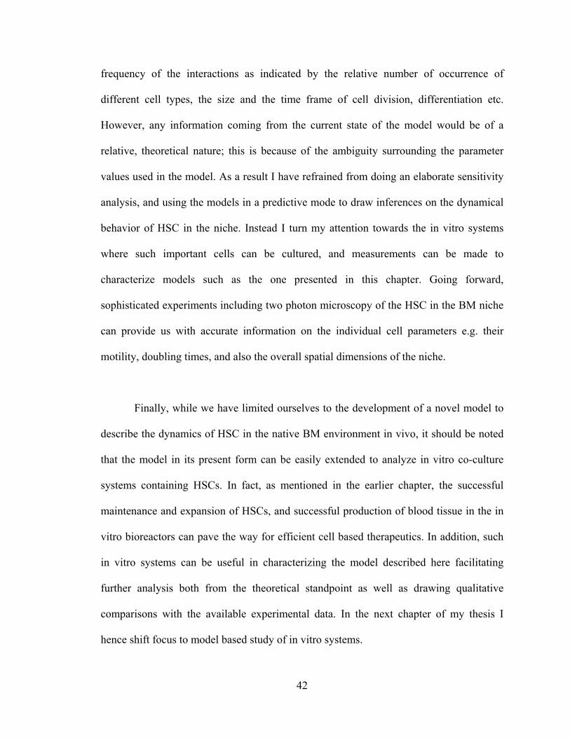
42
frequency of the interactions as indicated by the relative number of occurrence of
different cell types, the size and the time frame of cell division, differentiation etc.
However, any information coming from the current state of the model would be of a
relative, theoretical nature; this is because of the ambiguity surrounding the parameter
values used in the model. As a result I have refrained from doing an elaborate sensitivity
analysis, and using the models in a predictive mode to draw inferences on the dynamical
behavior of HSC in the niche. Instead I turn my attention towards the in vitro systems
where such important cells can be cultured, and measurements can be made to
characterize models such as the one presented in this chapter. Going forward,
sophisticated experiments including two photon microscopy of the HSC in the BM niche
can provide us with accurate information on the individual cell parameters e.g. their
motility, doubling times, and also the overall spatial dimensions of the niche.
Finally, while we have limited ourselves to the development of a novel model to
describe the dynamics of HSC in the native BM environment in vivo, it should be noted
that the model in its present form can be easily extended to analyze in vitro co-culture
systems containing HSCs. In fact, as mentioned in the earlier chapter, the successful
maintenance and expansion of HSCs, and successful production of blood tissue in the in
vitro bioreactors can pave the way for efficient cell based therapeutics. In addition, such
in vitro systems can be useful in characterizing the model described here facilitating
further analysis both from the theoretical standpoint as well as drawing qualitative
comparisons with the available experimental data. In the next chapter of my thesis I
hence shift focus to model based study of in vitro systems.

43
Table 2-A: List of variables and parameters for the HSC ABM Symbol Name/Description Base Value Lattice Size and Initial conditions
1 szgrid Grid Size 100 x 100 2 totcells Total Cells 150 3 prcell Individual cell composition varies 4 totmciter Total MC time 1000 (typical)
Quiescent cell activation 1 Nact Age before activation 152 Po Base activation by mechanism 1 0.053 k1 decay constant 2.994 Pact,b Base activation probability 0.05
Active Cell properties 1 NdivA Age before division 102 PdivA Base probability of division 0.253 PmoveA Probability of movement 0.54 Pdeact,b Base probability of deactivation 0.255 Pdiff,b Base probability of differentiation 0.3
Committed Cell properties 1 NdivD Age before division 52 PdivD Base probability of division 0.353 PmoveD Probability of movement 0.5

44
Figure 2.1: Classification of HSC interaction mechanisms in the BM niche. The various known regulatory mechanisms affecting the dynamics of HSCs inside the bone marrow are divided into three broad categories. 1. Direct Cell-Cell interaction symbolizing the interaction of the HSC with other cells like osteoblasts, CAR cells, etc. via direct adhesive contact. 2. Indirect cell-cell interaction wherein the cell influencing the HSC dynamics affect it via secretion of signaling molecules which act on the HSC through binding with cell surface receptors. 3. Systemic interactions, which include the regulatory mechanisms which act through systemic molecules circulated in the blood, eg. Oxygen, Granulocyte Colony Stimulating Factor (GCSF) etc.

45
Figure 2.2: Progression of hematopoietic stem cell states. Q, A and D stand for quiescent, active and committed progenitor (differentiated) stem cell state respectively. B denotes the migrated stem cell from the bone tissue to the blood via sinusoid. Single sided arrows denote irreversible change, while two sided arrows indicate reversible change. Self renewal is shown by an arrow pointing onto itself. Dashed arrow shows the movement of the committed progenitor from the BM tissue to blood. The probabilities of the transition used for the ABM are indicated on the arrows. Pact – Activation rate, or probability of transition from Q to A, Pdeact – probability of deactivation (A Q), Pdiff – probability of differentiation (A D). The probability Pmov represents the overall rate of movement of HSC type D into the blood stream. The probabilities are replaced by corresponding rate constants for the ODE model.
Q A D B Pact
Pdeact
Pdiv,Pdiv,
Pdiff [ Pmov]

46
Figure 2.3: 2-D Lattice model of Bone marrow for the agent based model. The left side of the lattice is assumed to be the endosteal surface, or the inner surface of the bone marrow, while the right side is assumed to be the sinusoid. The ‘agents’ as identified by the HSCs and support cells are initially randomly assigned to the grid points from which they evolve via the rules defined in the text. The color coded lattice points surrounding the support cells indicate the ‘sphere of influence’, (8 lattice points neighboring the cell) neighborhood of the cells wherein the secreted signaling molecule is assumed to act. The external growth factor has a concentration gradient, with decreasing concentration towards the bone side (left, shown in grey) and is depicted in the triangle with gradient shading.
HSC cells
Quiscent HSC
Active HSC
Commited Multipotent Progenitor
Support Cells
Cells secreting pro-differentiation factorsCells secreting anti-differentiation factorsOsteoblast like support cells with direct cell-cell interactionCAR cells like support cellswith direct cell-cell interaction
x
y

47
Figure 2.4: Implementation procedure for the ABM.
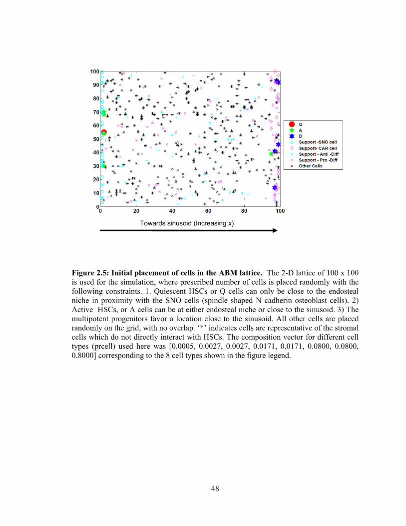
48
Figure 2.5: Initial placement of cells in the ABM lattice. The 2-D lattice of 100 x 100 is used for the simulation, where prescribed number of cells is placed randomly with the following constraints. 1. Quiescent HSCs or Q cells can only be close to the endosteal niche in proximity with the SNO cells (spindle shaped N cadherin osteoblast cells). 2) Active HSCs, or A cells can be at either endosteal niche or close to the sinusoid. 3) The multipotent progenitors favor a location close to the sinusoid. All other cells are placed randomly on the grid, with no overlap. ‘*’ indicates cells are representative of the stromal cells which do not directly interact with HSCs. The composition vector for different cell types (prcell) used here was [0.0005, 0.0027, 0.0027, 0.0171, 0.0171, 0.0800, 0.0800, 0.8000] corresponding to the 8 cell types shown in the figure legend.
Towards sinusoid (Increasing x)

49
Figure 2.6: Sample results for base case model. The model was simulated for a representative case with parameters corresponding to homeostasis. The initial conditions for the case were taken as per Wilson, et al. 2007. The steady state composition of the cell types were found to be slightly different from the reported values of relative abundance as reported in the paper, however the above result was found to be consistent for a wide range of parameters, indicative of a robust solution. The parameters used in the above simulation are as per table 2-A, and the initial composition is as per figure 2.5.

50
Figure 2.7: Simulating high dose chemotherapy. The model was simulated for a representative case of high dose chemotherapy by setting the population of the active and multipotent HSCs to zero, but retaining the stem cell. While it takes longer compared to the base case (fig. 2.6) to regenerate all the blood population from just the quiescent cell type, and the total blood production decreases, the model can predict reconstitution of the blood system as indicated by repopulation of the BM niche with HSCs of type A and D, along with the sustained production of multipotent progenitors. Note that the initial point for the system is not shown -- the first sample point in the system is for MC time = 10. The parameters used in the above simulation are as per table 2-A, and the initial composition is as per figure 2.5 but with zero probability of active or committed stem cells.

51
2.6. References
Abkowitz JL, Golinelli D, Harrison DE, Guttorp P. 2000. In vivo kinetics of murine hemopoietic stem cells. Blood 96:3399-3405.
Adams GB. 2008. Deconstructing the hematopoietic stem cell niche: revealing the therapeutic potential. Regen Med 3:523-530.
Adams GB, Scadden DT. 2006. The hematopoietic stem cell in its place. Nat Immunol 7:333-337.
Agur Z, Daniel Y, Ginosar Y. 2002. The universal properties of stem cells as pinpointed by a simple discrete model. J Math Biol 44:79-86.
Arai F, Hirao A, Suda T. 2005a. Regulation of hematopoiesis and its interaction with stem cell niches. Int J Hematol 82:371-376.
Arai F, Suda T. 2007. Maintenance of quiescent hematopoietic stem cells in the osteoblastic niche. Ann N Y Acad Sci 1106:41-53.
Belair J, Mackey MC, Mahaffy JM. 1995. Age-structured and two-delay models for erythropoiesis. Math Biosci 128:317-346.
Burt RK, Loh Y, Pearce W, Beohar N, Barr WG, Craig R, Wen Y, Rapp JA, Kessler J. 2008. Clinical applications of blood-derived and marrow-derived stem cells for nonmalignant diseases. JAMA 299:925-936.
Calvi LM. 2006. Osteoblastic activation in the hematopoietic stem cell niche. Ann N Y Acad Sci 1068:477-488.
Calvi LM, Adams GB, Weibrecht KW, Weber JM, Olson DP, Knight MC, Martin RP, Schipani E, Divieti P, Bringhurst FR, Milner LA, Kronenberg HM, Scadden DT. 2003. Osteoblastic cells regulate the haematopoietic stem cell niche. Nature 425:841-846.
Chan RJ, Yoder MC. 2004. The multiple facets of hematopoietic stem cells. Curr Neurovasc Res 1:197-206.
Colijn C, Mackey MC. 2005a. A mathematical model of hematopoiesis: II. Cyclical neutropenia. J Theor Biol 237:133-146.
Colijn C, Mackey MC. 2005b. A mathematical model of hematopoiesis--I. Periodic chronic myelogenous leukemia. J Theor Biol 237:117-132.
Conrad PD, Emerson SG. 1998. Ex vivo expansion of hematopoietic cells from umbilical cord blood for clinical transplantation. J Leukoc Biol 64:147-155.

52
Crocker PR, Morris L, Gordon S. 1988. Novel cell surface adhesion receptors involved in interactions between stromal macrophages and haematopoietic cells. J Cell Sci Suppl 9:185-206.
Devine SM, Lazarus HM, Emerson SG. 2003. Clinical application of hematopoietic progenitor cell expansion: current status and future prospects. Bone Marrow Transplant 31:241-252.
Dingli D, Pacheco JM. 2008. Some dynamic aspects of hematopoietic stem cells. Stem Cell Rev 4:57-64.
Frisch BJ, Porter RL, Calvi LM. 2008. Hematopoietic niche and bone meet. Curr Opin Support Palliat Care 2:211-217.
Gordon MY. 2008. Stem cells for regenerative medicine--biological attributes and clinical application. Exp Hematol 36:726-732.
Haurie C, Person R, Dale DC, Mackey MC. 1999. Hematopoietic dynamics in grey collies. Exp Hematol 27:1139-1148.
Huang X, Cho S, Spangrude GJ. 2007. Hematopoietic stem cells: generation and self-renewal. Cell Death Differ 14:1851-1859.
Kiel MJ, Iwashita T, Yilmaz OH, Morrison SJ. 2005. Spatial differences in hematopoiesis but not in stem cells indicate a lack of regional patterning in definitive hematopoietic stem cells. Dev Biol 283:29-39.
Kiel MJ, Morrison SJ. 2008. Uncertainty in the niches that maintain haematopoietic stem cells. Nat Rev Immunol 8:290-301.
Kiel MJ, Morrison SJ. 2006. Maintaining hematopoietic stem cells in the vascular niche. Immunity 25:862-864.
Kopp HG, Avecilla ST, Hooper AT, Rafii S. 2005. The bone marrow vascular niche: home of HSC differentiation and mobilization. Physiology (Bethesda) 20:349-356.
Kuehnle I, Goodell MA. 2002. The therapeutic potential of stem cells from adults. BMJ 325:372-376.
Li Z, Li L. 2006. Understanding hematopoietic stem-cell microenvironments. Trends Biochem Sci 31:589-595.
Loeffler M, Roeder I. 2004. Conceptual models to understand tissue stem cell organization. Curr Opin Hematol 11:81-87.
Loeffler M, Roeder I. 2002. Tissue stem cells: definition, plasticity, heterogeneity, self-organization and models--a conceptual approach. Cells Tissues Organs 171:8-26.
Mackey MC, Dormer P. 1982. Continuous maturation of proliferating erythroid precursors. Cell Tissue Kinet 15:381-392.
Mahaffy JM, Belair J, Mackey MC. 1998. Hematopoietic model with moving boundary condition and state dependent delay: applications in erythropoiesis. J Theor Biol 190:135-146.

53
Mantalaris A, Keng P, Bourne P, Chang AY, Wu JH. 1998. Engineering a human bone marrow model: a case study on ex vivo erythropoiesis. Biotechnol Prog 14:126-133.
Martinez-Agosto JA, Mikkola HK, Hartenstein V, Banerjee U. 2007. The hematopoietic stem cell and its niche: a comparative view. Genes Dev 21:3044-3060.
Moore KA. 2004. Recent advances in defining the hematopoietic stem cell niche. Curr Opin Hematol 11:107-111.
Moore KA, Lemischka IR. 2006. Stem cells and their niches. Science 311:1880-1885.
Morrison SJ, Spradling AC. 2008. Stem cells and niches: mechanisms that promote stem cell maintenance throughout life. Cell 132:598-611.
Murray L, DiGiusto D, Chen B, Chen S, Combs J, Conti A, Galy A, Negrin R, Tricot G, Tsukamoto A. 1994. Analysis of human hematopoietic stem cell populations. Blood Cells 20:364-9; discussion 369-70.
Nagy RD, Tsai BM, Wang M, Markel TA, Brown JW, Meldrum DR. 2005. Stem cell transplantation as a therapeutic approach to organ failure. J Surg Res 129:152-160.
Nemeth MJ, Bodine DM. 2007. Regulation of hematopoiesis and the hematopoietic stem cell niche by Wnt signaling pathways. Cell Res 17:746-758.
Olofsson TB. 1991. Growth regulation of hematopoietic cells. An overview. Acta Oncol 30:889-902.
Orlic D, Anderson S, Bodine DM. 1994. Biological properties of subpopulations of pluripotent hematopoietic stem cells enriched by elutriation and flow cytometry. Blood Cells 20:107-17; discussion 118-20.
Parmar K, Mauch P, Vergilio JA, Sackstein R, Down JD. 2007. Distribution of hematopoietic stem cells in the bone marrow according to regional hypoxia. Proc Natl Acad Sci U S A 104:5431-5436.
Porter RL, Calvi LM. 2008. Communications between bone cells and hematopoietic stem cells. Arch Biochem Biophys 473:193-200.
Raaijmakers MH, Scadden DT. 2008. Evolving concepts on the microenvironmental niche for hematopoietic stem cells. Curr Opin Hematol 15:301-306.
Rafii S, Lyden D. 2003. Therapeutic stem and progenitor cell transplantation for organ vascularization and regeneration. Nat Med 9:702-712.
Ratajczak MZ. 2008. Phenotypic and functional characterization of hematopoietic stem cells. Curr Opin Hematol 15:293-300.
Roeder I, Braesel K, Lorenz R, Loeffler M. 2007. Stem cell fate analysis revisited: interpretation of individual clone dynamics in the light of a new paradigm of stem cell organization. J Biomed Biotechnol 2007:84656.
Roeder I, Kamminga LM, Braesel K, Dontje B, de Haan G, Loeffler M. 2005. Competitive clonal hematopoiesis in mouse chimeras explained by a stochastic model of stem cell organization. Blood 105:609-616.

54
Roeder I, Loeffler M. 2002. A novel dynamic model of hematopoietic stem cell organization based on the concept of within-tissue plasticity. Exp Hematol 30:853-861.
Roeder I, Lorenz R. 2006. Asymmetry of stem cell fate and the potential impact of the niche: observations, simulations, and interpretations. Stem Cell Rev 2:171-180.
Ross J, Li L. 2006. Recent advances in understanding extrinsic control of hematopoietic stem cell fate. Curr Opin Hematol 13:237-242.
Schofield R. 1983. The stem cell system. Biomed Pharmacother 37:375-380.
Schroeder T. 2005. Tracking hematopoiesis at the single cell level. Ann N Y Acad Sci 1044:201-209.
Spradling A, Drummond-Barbosa D, Kai T. 2001. Stem cells find their niche. Nature 414:98-104.
Stier S, Ko Y, Forkert R, Lutz C, Neuhaus T, Grunewald E, Cheng T, Dombkowski D, Calvi LM, Rittling SR, Scadden DT. 2005. Osteopontin is a hematopoietic stem cell niche component that negatively regulates stem cell pool size. J Exp Med 201:1781-1791.
Suda T, Arai F, Hirao A. 2005a. Hematopoietic stem cells and their niche. Trends Immunol 26:426-433.
Suda T, Arai F, Shimmura S. 2005b. Regulation of stem cells in the niche. Cornea 24:S12-S17.
Sugiyama T, Kohara H, Noda M, Nagasawa T. 2006. Maintenance of the hematopoietic stem cell pool by CXCL12-CXCR4 chemokine signaling in bone marrow stromal cell niches. Immunity 25:977-988.
Taichman RS. 2005. Blood and bone: two tissues whose fates are intertwined to create the hematopoietic stem-cell niche. Blood 105:2631-2639.
Talibi Alaoui H, Yafia R. 2007. Stability and Hopf bifurcation in an approachable haematopoietic stem cells model. Math Biosci 206:176-184.
Tataria M, Perryman SV, Sylvester KG. 2006. Stem cells: tissue regeneration and cancer. Semin Pediatr Surg 15:284-292.
Tateno K, Minamino T, Miyauchi H, Kunieda T, Komuro I. 2006. Application of hematopoietic cells to therapeutic angiogenesis. Curr Pharm Des 12:557-563.
Trey JE, Kushner I. 1995. The acute phase response and the hematopoietic system: the role of cytokines. Crit Rev Oncol Hematol 21:1-18.
Troncale S, Tahi F, Campard D, Vannier JP, Guespin J. 2006. Modeling and simulation with Hybrid Functional Petri Nets of the role of interleukin-6 in human early haematopoiesis. Pac Symp Biocomput 427-438.
Wichmann HE, Loeffler M, Schmitz S. 1988. A concept of hemopoietic regulation and its biomathematical realization. Blood Cells 14:411-429.

55
Wilson A, Laurenti E, Oser G, van der Wath RC, Blanco-Bose W, Jaworski M, Offner S, Dunant CF, Eshkind L, Bockamp E, Lio P, Macdonald HR, Trumpp A. 2008. Hematopoietic stem cells reversibly switch from dormancy to self-renewal during homeostasis and repair. Cell 135:1118-1129.
Wilson A, Oser GM, Jaworski M, Blanco-Bose WE, Laurenti E, Adolphe C, Essers MA, Macdonald HR, Trumpp A. 2007. Dormant and self-renewing hematopoietic stem cells and their niches. Ann N Y Acad Sci 1106:64-75.
Wilson A, Trumpp A. 2006. Bone-marrow haematopoietic-stem-cell niches. Nat Rev Immunol 6:93-106.
Yin T, Li L. 2006. The stem cell niches in bone. J Clin Invest 116:1195-1201.
Zhang J, Niu C, Ye L, Huang H, He X, Tong WG, Ross J, Haug J, Johnson T, Feng JQ, Harris S, Wiedemann LM, Mishina Y, Li L. 2003. Identification of the haematopoietic stem cell niche and control of the niche size. Nature 425:836-841.
Zhu J, Emerson SG. 2004. A new bone to pick: osteoblasts and the haematopoietic stem-cell niche. Bioessays 26:595-599.

56
Chapter 3
3.Model-Based Analysis and Design of a Microchannel Reactor for
Tissue Engineering
Chapter Summary
Recently developed perfusion micro-bioreactors offer the promise of more
physiologic in vitro systems for tissue engineering. Successful application of such
bioreactors will require a method to characterize the bioreactor environment required to
elicit desired cell function. In this chapter, I present a mathematical model to describe
nutrient/growth factor transport and cell growth inside a microchannel bioreactor. Using
the model I first show that the nature of spatial gradients in nutrient gradients can be
controlled by both design and operating conditions and are a strong function of cell
uptake rates. Next I extend the model to investigate the spatial distributions of cell-
secreted soluble autocrine/paracrine growth factors in the bioreactor. Results show that
the convective transport associated with the continuous cell culture and possible media

57
recirculation can significantly alter the concentration distribution of the soluble signaling
molecules as compared to static culture experiments and hence needs special attention
when adapting static culture protocols for the bioreactor. Further, using an unsteady state
model, I find that spatial gradients in nutrient/growth factor concentrations can bring
about spatial variations in the cell density distribution inside the bioreactor which can
result in lowered working volume of the bioreactor. Finally, I show that the spatial and
nutrient limitations can dramatically affect the composition of a co-cultured cell
population. The results are significant for the development, design and optimization of
novel micro-channel systems for tissue engineering.
0.1. Introduction
Continuous cell culture protocols offer the promise of sufficient nutrient supply
along with continuous waste removal and hence are often preferred for culturing cells to
higher density or for developing tissue/organs in vitro. Perfusion systems are an
important class of continuous culture systems and are widely used to culture cells for
tissue engineering. Microchannel bioreactors have been developed to overcome the
difficulty associated with design and operation of large complex perfusion systems and to
have a larger and physiologically relevant surface to volume ratio. Advances in micro and
nanofabrication techniques have enabled the development of novel designs of
microchannel bioreactors to culture cells and create viable tissues like bone and cartilage
in the field of tissue engineering (Andersson & van den Berg, 2004). Micro-scale
perfusion systems have been reported for long term culture of hepatocytes, hematopoietic

58
cells, fibroblasts, muscle cell lines and osteoblasts (Allen, et al. 2005; Gu, et al. 2004;
Horner, et al. 1998; Koller, et al. 1993; Leclerc, et al. 2004; Leclerc, et al. 2006). Most of
the present approaches to develop such micro-scale systems for cell culture rely on
previous observations and large number of experimentation to optimize the bioreactor
and cell culture protocol in such systems. An important research topic in this field hence
relates to the ability to reproducibly control the cell behavior inside the bioreactor by
affecting the system design and operating variables.
A cell’s behavior is governed in part by the microenvironment within which the
cell resides. Apart from the physicochemical parameters such as pH, temperature,
nutrient concentration and mechanical stimuli, the bioreactor environment is also
regulated by the collection of cells residing in it through a complex network of cell-
secreted paracrine and autocrine soluble signals. For example, the epidermal growth
factor–receptor system in epithelial cells and fibroblasts plays a significant role in cell
expansion (Lauffenburger & Cozens, 1989) and the bone morphogenetic protein
signaling system is important in mesenchymal stem cell and chondrocyte differentiation
(Locker, et al. 2004; Rawadi, et al. 2003). A key factor to successful and reproducible
operation of microchannel bioreactors for clinical or fundamental studies hence involves
characterization of the microenvironment of the bioreactor.
Mathematical transport models can help to understand the relationships between
the bioreactor design and operating variables and the microenvironment inside the
bioreactor and can be especially useful to reduce the expensive and time consuming
experimentation. In particular, mathematical models hold promise for defining operating
windows, hypothesis testing, data interpretation, and optimization of these reactors.

59
Transport in perfusion bioreactors has been studied in various contexts and mathematical
transport models at various levels of complexity have been developed to characterize the
microenvironment for wide variety of bioreactor designs (Botchwey, et al. 2003; Ghanem
& Shuler, 2000; Galban & Locke, 1999; Horner, et al. 1998; Netti, et al. 2003; Williams,
et al. 2002). Transport of nutrients like oxygen has been extensively studied for various
reactor geometry and cell types (Allen & Bhatia, 2003; Horner, et al. 1998; Obradovic, et
al. 2000; Pathi & Locke, 2005; Roy, et al. 2001). Here, I build on the excellent
background of the available models and develop a generic model based design
framework for a perfusion-based microchannel bioreactor. I illustrate the utility of the
model by considering the example of cell proliferation inside a standard rectangular
channel bioreactor. I begin by presenting a generic, coupled nutrient transport and cell
proliferation model and analyze the model for various scenarios. First I present the results
of the steady state nutrient transport model with constant cell density and interpret them
to better understand the nature and existence of spatial gradients of nutrients and cell-
secreted autocrine/paracrine molecules inside the bioreactor. I consider also these
gradients when recirculation of used media is incorporated. Next I study the impact of
the nutrient gradients on the evolution of the cell population inside the bioreactor.
Subsequently I also investigate the implication of nutrient and spatial limitations on the
sustained viability and proliferation of a heterogeneous population of cells.

60
3.2. Methods
3.2.1. Model Formulation
The spatial and temporal changes in the concentration of various species of
interest (nutrients, metabolites, soluble exogenous and endogenous growth factors) inside
the bioreactor can be modeled using the reaction diffusion equation. The general mass
balance equation of soluble component i in the microenvironment of the bioreactor in
terms of concentration of soluble species (ci) in the media take the form
netiieiii RcDctc
,).(. +∇∇=∇+∂∂
u (3.1)
where Dei is the effective diffusivity of species i, u is the velocity profile of media inside
the bioreactor, and Ri,net represents the net volumetric uptake, secretion and degradation
rate for the species i and is dependent on the cell population density. In cases where the
cells are adherent and form a domain segregated from the flow layer, the volumetric
uptake vanishes in the species balance equation in the media domain.
The concentration distribution of various species given the reactor geometry, cell-
species interactions in terms of uptake and secretion rate, and also the cell population
distribution is the model output. It is important to note that the concentrations of nutrients
can affect the cell population dynamics and the cell population density in turn can affect
the distribution of nutrient. Quantitative models of cell behavior are, therefore, coupled to
the nutrient transport models. Furthermore, cell proliferation and differentiation behavior
is known to be affected by concentration levels of growth factors in various cell types
including hematopoietic cells and stem cells (e.g. Zandstra, et al. 1997). In such cases,
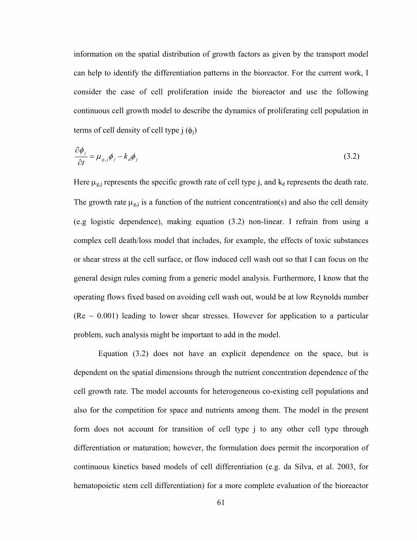
61
information on the spatial distribution of growth factors as given by the transport model
can help to identify the differentiation patterns in the bioreactor. For the current work, I
consider the case of cell proliferation inside the bioreactor and use the following
continuous cell growth model to describe the dynamics of proliferating cell population in
terms of cell density of cell type j (φj)
jdjjgj k
tφφμ
φ−=
∂
∂, (3.2)
Here μg,j represents the specific growth rate of cell type j, and kd represents the death rate.
The growth rate μg,j is a function of the nutrient concentration(s) and also the cell density
(e.g logistic dependence), making equation (3.2) non-linear. I refrain from using a
complex cell death/loss model that includes, for example, the effects of toxic substances
or shear stress at the cell surface, or flow induced cell wash out so that I can focus on the
general design rules coming from a generic model analysis. Furthermore, I know that the
operating flows fixed based on avoiding cell wash out, would be at low Reynolds number
(Re ~ 0.001) leading to lower shear stresses. However for application to a particular
problem, such analysis might be important to add in the model.
Equation (3.2) does not have an explicit dependence on the space, but is
dependent on the spatial dimensions through the nutrient concentration dependence of the
cell growth rate. The model accounts for heterogeneous co-existing cell populations and
also for the competition for space and nutrients among them. The model in the present
form does not account for transition of cell type j to any other cell type through
differentiation or maturation; however, the formulation does permit the incorporation of
continuous kinetics based models of cell differentiation (e.g. da Silva, et al. 2003, for
hematopoietic stem cell differentiation) for a more complete evaluation of the bioreactor

62
performance in advanced tissue engineering applications. Also, in the current study I
limit our model to non-motile cells, though one could include terms in the cell balance
equations to account for cell migration (Lauffenburger & Linderman, 1993).
In principle the solution of the above equations ((3.1)-(3.2)) can be obtained
numerically for any given ‘reaction rate’ Ri,net, μg,j , and kd and any reactor geometry. The
flow profile u can be obtained by using information on geometry and solving the relevant
fluid dynamics equations. However, information on the system can help us make some
vital simplifications in the model equations and hence make the solution process more
manageable. For the current work, I solve the model for the simple case of rectangular
microchannel reactor geometry as per figure 3.1, which shows the schematic of a
rectangular microchannel fabricated in PDMS using soft lithography technology or in
polycarbonate substrate by polymer micromachining. The media flows inside the channel
using a pumping device from a reservoir whose volume is usually much larger than the
channel volume (not shown). Although the current study is restricted to the geometry
shown in figure 3.1, the present simplification should hold for most microchannel
bioreactors culturing adherent cells, with no or minimal modifications. Also, it should be
noted that the model formulation and the subsequent development and coupling of the
transport equations with the cellular proliferation dynamics described here is general and
can be extended to other reactor geometries and co-ordinate systems.
I first consider a once through media flow without recirculation. We can simplify
the model for the rectangular microchannel based on the channel dimensions which
usually ensure that we can neglect the changes along the width (W), (W >> H) and hence
analyze the problem in 2-D. Further, due to the geometry we can adopt the Cartesian co-

63
ordinate system as shown in figure 3.1. Mammalian cells are likely to be adherent and be
selectively at the bottom of the channel either by themselves or encapsulated in
polymeric carriers dividing the channel into two domains. In the top domain, there are no
cells and the nutrients are transferred to the bottom cell domain by diffusion. We hence
hypothesize a geometry model where the cell domain of relatively small thickness δ is
adjacent to the unidirectional flow domain. With this assumption the mass balance
equation (3.1) in the flow domain is coupled to the cellular uptake/secretion through a
boundary condition at the interface and the volumetric uptake rate (Ri) vanishes. Further,
we can neglect the diffusion in the axial direction compared to the convective flux and
the volumetric degradation term to arrive at the following simplified equation for species
conservation in the flow domain:
2
2
ycD
xcu
tc i
eii
xi
∂∂
=∂∂
+∂∂
(3.3)
The flow profile in the reactor shown in figure 3.1 can be solved explicitly using the
Navier-Stokes equation with the incompressible assumption using a computational fluid
dynamics approach. However for the current work, considering the small conduit volume,
it is sufficient to assume a laminar flow profile in the flow domain. We assume a
unidirectional flow in the axial direction, and use the steady state velocity profile for
pressure driven flow between two plates for low Reynolds number given by
( )Hy
Hy
x uyu −= 16)( (3.4)
where <u> is the average velocity and H is the height of the flow domain, which is
approximately equal to the height of the microchannel for a cell mono-layer (δ<< H).

64
The general initial (equation (3.5) & (3.6)) and boundary conditions (equation (3.7)-(3.9))
for the set of equations ((3.2)-(3.4)) are
0)0,,( =yxci (3.5)
0)0( jj φφ = (3.6)
iUi
ie Ftxyc
D ,, ),0,( =∂∂
− (3.7)
iLi
ie FtHxyc
D ,, ),,( =∂∂
− (3.8)
ini ctyc =),,0( (3.9)
where φj0 denotes the initial (cell seeding) density of cell type j. The flux boundary
condition at the upper surface of the media flow layer (FU) is determined by the
permeability of the material in which the microchannel is etched out. PDMS (poly
dimethyl siloxane) can allow significant fluxes of gases across into the media due to its
high permeability, while diffusivity of gases in polycarbonate is not significant. For
specific consideration of gaseous components like oxygen, we can use a mass transfer co-
efficient (kl,a) to characterize the diffusion of gaseous nutrients from the PDMS layer,
where cisat denotes the solubility of component i in PDMS.
)(,, isat
ialiU cckF −= (3.10)
For other nutrients and growth factors we assume FU is negligible. The flux
boundary condition at the lower surface (equation (2.8)) of the flow layer (FL) is
determined by the uptake rate of cells and the cell density, and hence is coupled with the

65
cell population balance equation. The axial boundary condition at the inlet is the Dirichlet
type (equation (3.9)), with specified concentration.
Recirculation of media in the bioreactor offers the promise to retain the cell-
secreted growth factors, and can be achieved in two possible manners as shown in the
figure 3.2. In either case, we need to modify the boundary condition at the reactor inlet
(equation (3.9)) to account for the recirculation, which can be done by using the mass
balance equations for the recycle loop. For example in case of scheme B for constant inlet
velocity, defining the recirculation ratio r as the fraction of the outlet flow which is
recycled back, the inlet concentration (c*) can be calculated from the media
concentration (cin) and the reactor outlet concentration (cout) for species i
outiinii rccrc ,,* )1( +−= (3.11)
3.2.2. Constitutive Relationships for uptake/secretion and cell proliferation rates
The chemical species under consideration could be essential growth factors,
nutrients, or the products of cell metabolic activities. Most nutrient or metabolite uptake
rates are known to follow saturation kinetics and modeled as Michaelis-Menten (MM)
kinetics for a wide variety of cells and nutrients (Allen & Bhatia, 2003; Ben-Abraham, et
al. 2003; Obradovic, et al. 2000), and the values of the MM parameters can be measured
from experiments done on static culture protocols. The mathematical expression of the
specific uptake rate for species i by cell type j (Rup,ij) would thus take the form
⎟⎟⎠
⎞⎜⎜⎝
⎛
+=
iijm
iijijup cK
cVR
,
max,, (3.12)

66
Vmax,ij and Km,ij are the MM parameters. The actual uptake rate depends on the specific
uptake rate and the local cell density and it can be assumed that the actual uptake rate is
directly proportional to the cell density (Jorjani & Ozturk, 1999). The corresponding flux
boundary condition at the cell-media interface for a general case with N cell types hence
would be ∑∑==
⎟⎟⎠
⎞⎜⎜⎝
⎛
+==
N
jj
iijm
iijj
N
jijupiL cK
cVRF
1 ,
max,
1,, φφ (3.13)
The model in its present form can also be extended for cell-secreted molecules,
e.g. growth factors and other chemical signaling molecules which may act in an autocrine
or paracrine manner and play an important role in governing cell viability and function.
The mathematical modeling of autocrine growth factor secretion and their regulation has
been studied using various mathematical approaches to understand the associated
signaling pathways (Bhalla & Iyengar, 1999; Shavartsman, et al. 2001), particularly for
the EGF system (Wiley, et al. 2003). However, for the present study we consider an
autocrine growth factor affecting the cell growth rate, and consider the case where the
secretion of the growth factor is constant for each cell (i.e the secretion is not regulated),
and is taken up by the cells in a dose dependent manner described by MM kinetics. We
use this simplistic set-up to understand the general guiding principles for bioreactor
design and optimization, particularly for reactors with recirculation. For the case of a
soluble growth factor described above, the flux conditions at the domain bottom (y = H)
for homogenous population of a single cell type would be
φφ ⎟⎟⎠
⎞⎜⎜⎝
⎛
+−=
gfgfm
gfgfgfgfL cK
cVqF
,
max,, (3.14)
The subscripts on the cell density φ have been dropped as we consider just a single cell
type for this case. qgf represents the specific rate of secretion of the autocrine growth

67
factor while Vmax,gf and Km,gf are the uptake parameters. Important simplifying
assumptions in the above model for cell secreted soluble growth factor are that within the
cell domain the uptake of the species is spontaneous and without any further diffusive
resistance and that the secretion rate (qgf) is constant.
We use a logistic cell growth model with substrate inhibition kinetics for growth rate
dependency on nutrient concentration (Pathi, et al. 2005). The later is chosen to reflect
the impact of nutrients like oxygen on cell growth as it is known that conditions with high
concentration of oxygen can be detrimental for cell growth, while lower concentrations
can decrease the growth rate. The general expression for cell growth for cell type j,
assuming limiting nutrient species i, hence can be taken as:
∏∑
⎟⎟
⎠
⎞
⎜⎜
⎝
⎛
++⎟⎟⎟
⎠
⎞
⎜⎜⎜
⎝
⎛
−=i iijiij
iijjj
jg ckck
ck2
32
1
maxmax, 1
1φ
φμμ (3.15)
where, φmax is the maximum cell density or carrying capacity of the system, and ci
represents the concentration of limiting nutrient species. The growth model parameters
k1,ij k2,ij and k3,ij represent the impact of concentration of nutrient species i on the growth
of cell type j. A value of parameter k,3,ij close to zero indicates the standard Monod type
kinetics, while a larger value indicates detrimental effect of the nutrient on cell growth at
higher concentrations. The summation is carried over all the cell types, and the product is
over all the limiting nutrient/growth factor species.
3.2.3. Solution to model equations
We solve the system of equations (equation (3.2) - (3.9)) in a non-dimensional
framework as a convenient way to explore the large number of parameters in a systematic

68
manner. Table 3-A gives the non-dimensionalization scheme for variables and the key
dimensionless groups involved. The model can be solved for various cases of interest,
making appropriate changes in the general model equations. The model equations in its
working/non-dimensional form for the general case as well as the specific cases described
below are tabulated in Table-3B.
The partial differential equation ((3.1) or (3.3)) governing the nutrient/growth
factor distribution can be decoupled from the cell proliferation dynamics equation (2.2)
by assuming constant cell density for results which are valid for short times. Further, the
model equations can be solved at steady state to arrive at the steady state spatial
distribution of nutrient and/or growth factor inside the reactor for a given cell population
density. Solving the fully coupled unsteady state model in its full form (equations (2.2)-
(2.9)) is computationally expensive, as the time step required to solve the species
conservation equation is much smaller than that required by the cell proliferation
equation. The cell proliferation time scale characterized by the doubling time (td) is of the
order of hours while the residence time (tr) of the media inside the reactor is of the order
of minutes (tr = L/<u>). However, this knowledge leads to a useful approximation of the
model equations where we can assume that while considering the dynamics of cell
proliferation, the concentration field is always at the steady state. This pseudo steady
state analysis is valid for small values of λ (defined as the ratio of two time scales, λ = =
tr/td = L/ (td<u>)) and enables us to solve the cell population balance equation in its
unsteady form, while the species conservation equation can be solved at steady state. We
use these results to analyze the effect of nutrient gradients on cell density distribution and
vice-versa.

69
The dimensionless analysis broadens the applicability of the model results and
undermines the need to get the actual parameter values for all possible experiments for
the present study. Nevertheless, the model parameters for simulation are chosen to reflect
literature data whenever available. We use the published data for reactor geometry and
oxygen consumption of hepatocytes (Allen & Bhatia, 2003; Roy, et al. 2001) for our
calculations. Further, the oxygen uptake is reported to vary up to 2 orders of magnitude
for wide variety of cell types (Guarino, et al. 2004) and hence we vary the parameter Da
to simulate the condition corresponding to different cell types. Similarly, the uptake of
the cell secreted autocrine factor is varied based on estimation of the range of autocrine
ligand secretion rates as reported earlier (Oehrtman, et al. 1998). The base case values of
the parameters as estimated from literature cited above are tabulated in Table3-C.
Model equations were solved numerically using finite element software FEMLAB
(v. 3, Consol AB Inc). Model equations in their non-dimensional form (Table 3-B) were
solved for a representative set of parameters (Table 3-C). We study the effect of
recirculation by simultaneously solving the species balance partial differential (equations
(3.3)-(3.9)) and the mass balance equations in the recycle loop (equation (3.10)) in an
iterative manner. Analytical solutions for the given set of equations can be found for a
uniform velocity profile and zero order oxygen flux and constant cell density, and these
were compared to the numerical solutions to confirm the sanctity of the numerical
solution procedure. Furthermore, steady state model results for the case of constant cell
density and without recirculation (case (b) of table 3-B, with Sh = 0) were compared and

70
were found to be in agreement with the published numerical solutions for the outlet
concentration of oxygen in a flat bed culture of rat hepatocytes (Allen & Bhatia, 2003).
0.3. Results and discussion
3.3.1. Steady state model analysis at constant cell density: nutrient distribution
A good measure of the performance of the bioreactor is the ability of the
bioreactor to sustain a cell population and provide it with the required nutrients to ensure
desired cell function and viability. The depletion of nutrient from the media by cell
uptake as it flows downstream of the reactor creates axial nutrient gradients on the cell-
media interface which may not be desirable. Non-dimensionalization of the model
equations (Table 3-B) shows that two dimensionless groups are important in determining
the concentration distribution of the species inside the bioreactor, Pe/α (= <u>H2/(DeL))
and the Damkohler number (Da=VmaxφH/Decin). The dimensionless group Pe signifies the
Peclet number ( Pe = <u>H/De), and it represents the ratio of convective transfer of
species in the axial direction to the diffusive flux within the channel directed towards the
lower end of the channel, i.e towards the cell domain. The Damkohler number is a
measure of relative rates of the total cellular uptake and the diffusive flux from the bulk
media. The value of Da is largely dependent on the cell type and its metabolic state, and
also includes the cell density. For example here, the value of Da = 0.21 for oxygen
transport corresponds to the rat hepatocytes (Vmax=3.8 × 10⁻¹⁶ molcell-1s-1) cultured at a
cell density of 2.1× 10⁹ cells/m2.

71
We first simulate the condition of the reactor for a constant cell density. Figure
3.3 shows the effect of the parameters Pe/α and Da on the non dimensional outlet
concentration (Cout) of the nutrient species at the cell-media interface (X =1, Y=1). The
outlet concentration is scaled to the inlet concentration, and hence the dimensionless
concentration (C) of nutrient at the inlet is equal to unity, making (1- Cout) the effective
concentration drop or axial gradient inside the bioreactor. For a given cell density and
cellular uptake rate (fixed Da), as we increase the parameter Pe/α, the convective flux
dominates and the outlet concentration of the nutrient increases. The diffusive flux of
nutrient across to the cell domain is also higher due to higher concentrations in the media
domain (not shown). Increased convective flux signifies higher influx rates, and also the
fact that nutrients are pushed through the reactor faster than they can diffuse and be
consumed by the cells. We hence conclude that increasing flow rate or changing the
operating parameters so as to selectively increase Pe/α can lead to decreasing the axial
gradients inside the bioreactor. Further, for a given Pe/α, an increase in Da is reflective of
the increased rates of consumption by cells, and hence a corresponding decrease in the
outlet concentration or increased nutrient gradient is observed.
Further useful conclusions regarding the design and operation of the bioreactor
can be drawn from figure 3.3. Of the variables included in the two dimensionless groups,
we can roughly classify the media flow rate and the inlet concentration of the nutrient
(<u>, and cin) as operational variables. For example, during the operation of the
bioreactor, the media flow rate can be used for controlling the concentration gradients of
the nutrient so that the concentration of a particular nutrient does not fall below a certain

72
threshold value inside the reactor. However, the choice of the media flow rate is usually
limited by the fact that cells cannot be subjected to high levels of flow associated shear
stress, and hence the media flow rate can only be used as a fine control. Nevertheless, the
graph clearly also gives the options of designing the reactor geometry variables (L, H)
which can have similar effect on the concentration gradient. At the design stage, we can
determine, from the graph, the design variables for culturing cells to a given cell density
so that the concentration of the nutrient is always above the prescribed minimum value.
Conversely, for a given reactor geometry and maximum flow rate (e.g. determined by the
reactor limitations and shear stress considerations), the model results can be used to
estimate the maximum value of the cell density the bioreactor can support by estimating
the value of Da for the desired outlet concentration of nutrient , given the value of Pe/α.
The results of figure 3.3 can also be used to quickly answer non-trivial design
questions. For example, the effect of length on the axial gradients is fairly intuitive, as
increasing the length will increase the gradients by decreasing the parameter Pe/α, but the
effect of channel height cannot be readily predicted. The group Pe/α has a quadratic
dependence on the height, while the Da is directly proportional to height. Hence
increasing the height of the channel will increase Pe/α, shifting the operating point on the
curve on figure 3.3 towards the right, and increase Da, shifting the operating point down,
but more to the right than down. Thus depending on the location of the original operating
point, increase in height can decrease, increase or have negligible effect on the outlet
concentration of the nutrient. For example, as per figure 3.3, if we were to double the
height when operating at a value of Da=1.05, and Pe/α value less than 1, the new
operating point will be shifted to the curve with Da = 2.1, and a Pe/α value of about 4,

73
increasing the outlet concentration. If, however, the original operating point was close to
Pe/α =2, we would see an effective decrease in the outlet concentration, or increased
axial gradient. In general, the channel height can be used to adjust the nutrient
distribution in the reactor and the effect of changing the height on the cell culture can
give us useful insights on the operating point of the bioreactor.
In addition to the supply of nutrients by the media flow, important nutrients like
oxygen can be supplied by surface aerators or membrane oxygenators (Roy, et al. 2001).
We extend the results presented by Roy, et al. in the context of operation of the bioreactor
as done. Figure 3.4 shows the dimensionless outlet concentration of gaseous nutrient for
the case of non-zero flux from the PDMS layer. The magnitude of diffusion from the
PDMS is governed by the value of the Sherwood number (Sh) defined as the ratio of the
diffusive transfer rate from the PDMS to the diffusion rate in the media. (Sh = kl,aH/De).
The results indicate that the diffusive flux from the membrane or PDMS layers is
important for low values of Pe/α, while at higher values of Pe/α convective flux
dominates and diffusion from boundary does not affect the concentration of the species at
the cell interface. The above results can be interpreted as follows: For the case of slow
diffusion of the species across the media, and/or large channel heights, the molecules of
the species are driven out by the media flow faster than they then diffuse to the cell layer,
and hence for higher values of Pe/α (= <u>H2/(DeL)) we see a corresponding saturating
behavior of the concentration variable for various values of Sh. Clearly the use of highly
permeable material or external supply using membranes cannot help in such cases, and a
significant alteration in the design or operation of the bioreactor is warranted.
Specifically, the results indicate that the model can be used to infer the optimal design to

74
balance the nutrient delivery using the flow and surface transfer and keep a desired level
of nutrient inside the bioreactor.
3.3.2. Steady state model analysis at constant cell density: Transport of cell-secreted
growth factors
We illustrate the use of model analysis for soluble cell-secreted growth factors by
considering a simple case of a single representative growth factor which acts in an
autocrine manner in a homogeneous cell population. Non-dimensionalization of the
model (Table 3-B) gives two relevant Damkohler number groups: Dain (qgf φH/(DKm)),
associated with the influx of the soluble growth factor to the flow domain by the cells,
and Daup (Vmax,gfφH/(DKm)), associated with the uptake as described above. Both
dimensionless groups represent the ratio of rates of secretion/uptake to the diffusive flux
from the flow domain. Importantly, we define the parameter γ as the ratio of the influx to
uptake Damkohler numbers (γ=Dain/Daup). Larger values of γ are indicative of ample
secretion of the growth factor and therefore the growth factor receptors are most likely
saturated and loss of growth factor due to convective transfer may not be important.
However, when γ is closer to unity, the loss of growth factor by media flow can affect the
cell culture. Also, even when γ is large, the convective losses might dominate the
secretion rates at high Peclet numbers, and the growth factor concentration can drop
considerably.

75
Figure 3.5 shows the effect of the operating variable group Pe/α on the outlet
concentration of the cell secreted autocrine growth factor. As we increase the media flow,
or change other parameters in the group (see Table I) so as to increase the value of Pe/α,
we are effectively pushing larger volumes of the media in the given time, thereby
decreasing the concentration of the autocrine growth factor. This argument is valid
irrespective of the value of γ or Da; however, the magnitude of the decrease depends on
the values of γ and Da. Also, increasing the value of γ increases the rate of secretion
compared to the uptake, and hence the outlet concentration of the growth factor increases
as γ is increased. Similarly, an increase in the value of Da is indicative of an increased
uptake/secretion rate compared to diffusive flux, and hence increased Da increases the
outlet concentration of the growth factor.
The results can be interpreted in a slightly different manner by comparing the
continuous culture experiment modeled here with a static culture protocol. For a static
culture all of the growth factor is retained inside the media until the media is changed,
typically every 2-3 days. For the continuous culture the media is continually replaced,
and there is loss of the cell-secreted soluble growth factor through the media outflow.
One way to compare these two protocols is by analyzing the fraction of autocrine growth
factor lost. We can calculate the fraction of autocrine growth factor lost in the continuous
culture experiment by dividing the integrated convective flux at the outlet to the total rate
of production of the growth factor inside the reactor. Mathematically it is equivalent to
the following equation
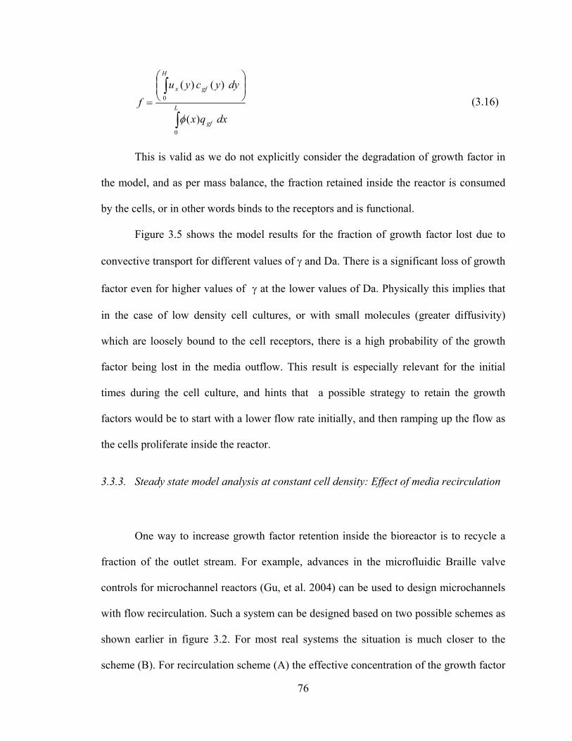
76
∫
∫ ⎟⎟⎠
⎞⎜⎜⎝
⎛
= L
gf
H
gfx
dxqx
dyycyuf
0
0
)(
)()(
φ (3.16)
This is valid as we do not explicitly consider the degradation of growth factor in
the model, and as per mass balance, the fraction retained inside the reactor is consumed
by the cells, or in other words binds to the receptors and is functional.
Figure 3.5 shows the model results for the fraction of growth factor lost due to
convective transport for different values of γ and Da. There is a significant loss of growth
factor even for higher values of γ at the lower values of Da. Physically this implies that
in the case of low density cell cultures, or with small molecules (greater diffusivity)
which are loosely bound to the cell receptors, there is a high probability of the growth
factor being lost in the media outflow. This result is especially relevant for the initial
times during the cell culture, and hints that a possible strategy to retain the growth
factors would be to start with a lower flow rate initially, and then ramping up the flow as
the cells proliferate inside the reactor.
3.3.3. Steady state model analysis at constant cell density: Effect of media recirculation
One way to increase growth factor retention inside the bioreactor is to recycle a
fraction of the outlet stream. For example, advances in the microfluidic Braille valve
controls for microchannel reactors (Gu, et al. 2004) can be used to design microchannels
with flow recirculation. Such a system can be designed based on two possible schemes as
shown earlier in figure 3.2. For most real systems the situation is much closer to the
scheme (B). For recirculation scheme (A) the effective concentration of the growth factor

77
inside the reactor would be a balance of the increasing effect brought about by
recirculation and the decreasing effect due to the increased flow as per figure 3.5.
Alternatively, scheme (B) would tend to increase the concentration without any flow
effect. Furthermore, model analysis of scheme (B) can give a clear understanding of the
effect of recirculation without the confounding effects of a changing effective flow rate
inside the reactor, and so we study the effect of recirculation as per scheme (B).
Figure 3.7a shows the effect of the recirculation ratio r on the axial distribution of
the growth factor concentration at the cell-media interface for scheme (B) for the case of
γ=1. As expected, an increased recirculation ratio increases the concentration of the
autocrine growth factor inside the reactor and also it is seen that the concentration of the
autocrine growth factor builds up as we move downstream. However it should be
considered that recycling the exit fluid will also, however, mean that effective
concentration of the nutrient in the bioreactor is lowered. Figure 3.7b shows the spatial
distribution of the nutrient concentration for different recirculation ratios for same
operating conditions. Clearly, the larger the recirculation ratio, the lower is the nutrient
concentration inside the reactor. While we gain in terms of growth factor retention by
recirculation, a key nutrient may be depleted. The choice of the fraction to recycle hence
will have to be optimized for adequate retention of growth factor and also adequate
nutrient availability. Figure 3.8 shows the effect of recirculation on both the growth
factor retained inside the reactor and the nutrient outlet concentration for a conservative
case of γ=1 and a constant Pe/α. The optimal recirculation ratio can be determined by
predefined thresholds of nutrient/growth factor concentrations that are required for
functioning of the cells. Clearly when both the criteria are not met with one operating
78
condition, it would be required to supplement the media with extra growth factor or
nutrient. Furthermore, 3.8 shows the effect of the Damkohler number on the location of
the optimal recirculation ratio. Clearly with larger values of Da, the depletion of the
nutrient is more significant, and so the optimal recirculation ratio would tend to be lower
than when operating at higher cell densities. Physically, it can be argued from the results
that cell culture processes with larger cell density can be controlled more effectively with
small amounts of recirculation for cases where the value of γ is close to unity.
Cell growth and differentiation is mostly governed by cell secreted molecules, for
example the role of BMP in osteoblast differentiation is well known. Furthermore
experiments with osteoblastic cell lines in microfluidic environment have revealed the
influence of media flow on the cell growth and differentiation (Leclerc et al, 2005).
Although the actual effect of growth factor washout cannot be interpreted from such
experiments due to confounding of various processes including cell-wash out, regulation
of growth factor secretion etc, we believe that going forward model based recirculation
strategies can help to efficiently cue the cells towards the desired behavior.
3.3.4. Unsteady state model analysis: Long term cell proliferation
The long term performance of the bioreactor can be studied by understanding the
cell response to the nutrient gradients inside the bioreactor. Figure 3.9 depicts the results
of the solution of the coupled model with cell proliferation and the nutrient mass balance.
The model results indicate that the nutrient gradients inside the bioreactor can affect the
cell density distribution as cells proliferate inside the reactor. The higher concentration of
the nutrient at the inlet favors rapid proliferation of the cells near upstream, which acts to

79
deplete the nutrient and thus the nutrient concentration decreases along the axial
dimension of the reactor. The cells downstream hence proliferate slowly, and in extreme
cases can also suffer from starvation resulting in cell death. Clearly, then, gradients in
nutrient concentration can limit the working volume of the reactor channel by selectively
proliferating only upstream sections of the channel. From figure 3.3, we know that the
nutrient gradients can be minimized by for example, increasing the inlet concentration
(decreasing Da), or increasing the flow rate (increasing Pe/α). More interestingly, it may
be sometimes desirable to have gradients of chemical signaling molecules inside the
channel; for example in applications involving tissue engineering of liver, the gradients
of oxygen inside the reactor can simulate an in vitro model of zonation which is
important in developing bio-artificial liver and also for studying drug metabolism in liver
(Allen & Bhatia, 2003). In this scenario, the model could also be used to develop an
operating strategy to ensure that all cells proliferate equally during the initial proliferation
stage, while appropriate environments can be provided at a later stage of development by
changing the operating conditions inside the reactor.
Experimental observations (Gu, et al. 2004) indicate that even when initially the
cells are seeded uniformly inside the channel, the cell density distribution evolves a
dependence on the axial dimension, presumably in response to the gradients of nutrient
concentrations inside the reactor as indicated by the model results presented here. Using
the information on cell characteristics and the model results as shown in 3.3, one could
design and operate the reactor to avoid cell density gradients in the reactor for such
systems. The model results can also provide useful diagnostic tools to better understand
the performance of the bioreactor. A difference in the immobilized cell density at the

80
upstream and downstream of the reactor could be indicative of the fact that there are
significant gradients in essential nutrients or growth factors (or possibly toxic metabolic
products) inside the reactor. Furthermore, higher upstream cell density probably means
that there are nutrient(s) limitations inside the reactor and hence the operating point
should be shifted so as to minimize the gradients inside the reactor. Alternatively, if the
cell density is higher downstream in the reactor, it could mean that an autocrine growth
factor is limiting or that there is a possible toxic effect of higher concentration of any
nutrient at the inlet, and hence a model based recirculation strategy based on figure 3.8
could be devised.
3.3.5. Effect of cell type heterogeneity
Novel tissue engineering applications involve the co-culturing of different cell
types to achieve a functional tissue or organ. The introduction of different cell types
inside the bioreactor can introduce several levels of complexities in the design and
operation of the bioreactor in terms of sustained viability, growth and function of all the
cell types. We demonstrate the use of the model by considering the case of cell
proliferation in a co-culture with two cell types with doubling times td1 and td2, and we
assume that there is a maximum carrying capacity of the reactor (Φ1 + Φ2)max.
Both nutrient and spatial limitations govern the time evolution of the individual
cell densities, and in general the composition of the cell co-culture will change over time.
As shown in figure 3.9 for the case of td1=16 h and t d2=32 h, when the initial cell
population is an equal mix of cell types 1 and 2 (Φ2/Φ1=1), the conditions favor the
proliferation of cell type 1 and the cell population becomes largely of cell type 1 over

81
time. Thus to achieve a long term co-culture of a specified composition, one must
determine the appropriate initial mix to seed the reactor. The model can be used to
calculate the initial cell densities of the individual cell type required to achieve the
specified target composition at confluence. For example, in the case described above in
figure 3.10, if we want equal proportion of both cell types, starting with initial cell
compositions of Φ2/Φ1~5, one can achieve a target composition of Φ2/Φ1~1.
Although the full set of model equations must be solved to arrive at the plots
shown in figure 3.9, one can obtain a useful estimate of the required initial densities of
cells to achieve a final target composition by considering spatial, but not nutrient,
limitations in the reactor (Table 3-B, case (e)). Indeed, assuming negligible cell death, we
can simplify the ODE to arrive at the following relationship between the cell densities of
the two types.
2
1
2
1
ΦΦ
=ΦΦ
add
(3.17)
where a is the ratio of the doubling times of the two cells types given by td2/td1. We have
used the fact that the growth rate in the exponential regime follows the simple
relationship μg,max = ln(2)/td. Equation (3.15) can be used to estimate the initial
composition required to achieve a target final composition in a simple manner without
going through the full model solution. For the present case, we can back calculate the
initial conditions required to achieve the final target composition (~ Φ1 = Φ2 = 5) for the
given value of parameter a (=2) which gives the value of Φ1,0 = 0.15, and Φ2,0 = 0.85
resulting in the ratio (Φ2/Φ1)τ=0 = 5.67. Hence, it can be seen that even in the presence of

82
the nutrient gradients (figure 3.9b), the estimate from the ODE model using the analysis
described above remains reasonable.
The ability to maintain a composition of cells in proliferating cell cultures can
prove to be crucial in some important tissue engineering applications, e.g. in culturing
primary cells consisting of adult stem cells (Koller, et al. 1997). Primary cells are
inherently heterogeneous and adult stem cells form a very small percentage (< 0.001%)
of the cell population. The survival and controlled differentiation of these stem cells may
require the presence of multiple cell types in a reactor. Model based analysis as described
here can help to understand and overcome some of the problems encountered in such
culture processes.
0.4. Conclusion
Microchannel reactors for tissue engineering are associated with a vast and
largely uncharacterized design space and the design and operation of these bioreactors
can be aided by mathematical modeling. We present here a coupled model for
nutrient/growth factor distribution and cell proliferation in the microchannel bioreactor
and use it to show how operating parameters (e.g. flow rate, recirculation) and design
parameters (e.g. channel height) can influence the cell growth in the bioreactor. We
believe that models formulated on the basis of known qualitative or quantitative
information on the systems of interest can be used to narrow the experimental design
space, and can help in design and optimization of the bioreactors along with offering an
insight into the fundamental functioning of such systems.

83
Table 3-A: Non-dimensional variables and groups
Dimensional variable/parameter Description Dimensionless
variable/parameter Definition
c Concentration C
C = c/cin OR
C = c/Km
x Axial distance X X = x/L
y Height dimension Y Y = y/H
ux Velocity U U = ux/<u>
t Time τ τ = t/td
φ Cell density Φ Φ = φ/φ0
k1 Cell growth model parameter K1 K1 = k1*cin
k2 Cell growth model parameter K2 K2 = k2*cin
k3 Cell growth model parameter K3 K3 = k3*(cin)2
Dimensionless groups Description Definition
α Geometric ratio α = L/H
Pe Peclet number Pe = <u>H/De
Da
Damkohler Number
Da = VmaxφH/(Decin) (Nutrient) OR
Daup = VmaxφH/(DeKm) (Growth factor, uptake) OR
Dain = qφH/(DeKm) (Growth factor, secretion)
Sh Sherwood Number Sh = kl,aH/De
γ Ratio of influx to
uptake of growth factor γ = Dain/Daup = q/Vmax
λ Ratio of time scales λ = L/ (td<u>)

84
Table 3-B: Model equations and boundary conditions
# Case Working/Dimensionless Equations Initial and boundary conditions
a General case
2
2
YC
PeXC
UC iii
∂
∂=
∂∂
+∂∂ α
τλ
jddjjgdj tkt Φ−Φ=
∂
Φ∂)()( ,μ
τ
Ci (X,Y,0) = 0
Ci (0,Y,τ) = Ci,in
)(),0,( CCShXYC sati −=
∂∂
τ
⎟⎠⎞
⎜⎝⎛ +
Φ=
∂∂
),1,(*
),(),1,(),1,(τ
τττxC
cK
XXCDaXYC
m
i1
Φj (X,0) = 1
b Steady state with constant cell density (Nutrient)
2
2
YC
PeXC
U ii
∂∂
=∂∂ α
Φ = 1
Ci (0,Y,τ) =1
0),0,( =∂∂
τXYCi OR for Gaseous nutrient
)(),0,( CCShXYC sati −=
∂∂
τ
⎟⎟⎠
⎞⎜⎜⎝
⎛+
=∂∂
),1,(
),1,(),1,(τ
ττxC
cK
XCDaXYC
in
m
i
c Steady state with constant cell density (Autocrine growth factor)
2
2
YC
PeXC
U ii
∂∂
=∂∂ α
Φ = 1
Ci (0,Y,τ) =0
0),0,( =∂∂
τXYCi
( ) ⎥⎦
⎤⎢⎣
⎡−
+=
∂∂
γτ
ττ),1,(1
),1,(),1,(xC
XCDaXYCi
d Pseudo steady state
2
2
YC
PeXC
U ii
∂∂
=∂∂ α
jddjjgdj tkt Φ−Φ=
∂
Φ∂)()( ,μ
τ
Ci (0,Y,τ) = Ci,in
0),0,( =∂∂
τXYCi
⎟⎟⎠
⎞⎜⎜⎝
⎛+
=∂∂
),1,(
),1,(),1,(τ
ττxC
cK
XCDaXYC
in
m
i
Φ(X,0) = 1 e Spatial limitations
only jddjjgdj tkt Φ−Φ=
∂
Φ∂)()( ,μ
τ
Φj (X,0) = 1
1 c* is the concentration scaling variable. It is equal to the inlet concentration cin for nutrients, and equal to MM parameter Km for the autocrine growth factor.
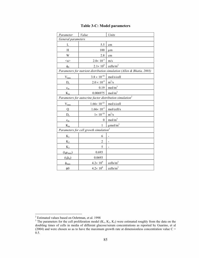
85
Table 3-C: Model parameters
Parameter Value Units General parameters
L 5.5 cm
H 100 μm
W 2.8 cm
<u> 2.0× 10⁻³ m/s
φ0 2.1× 10⁹ cells/m2 Parameters for nutrient distribution simulation (Allen & Bhatia, 2003)
Vmax 3.8 × 10-16 mol/s/cell
De 2.0 × 10⁻⁹ m2/s
cin 0.19 mol/m3
Km 0.006975 mol/m3 Parameters for autocrine factor distribution simulation2
Vmax 1.66× 10-22 mol/s/cell
Q 1.66× 10⁻² mol/cell/s
De 1× 10⁻¹⁰ m2/s
cin 0 mol/m3
Km 1 μmol/m3 Parameters for cell growth simulation3
K1 6 -
K2 2 -
K3 5 -
(tdμmax) 0.693
(tdkd) 0.0693
φmax 4.2× 109 cells/m2
φ0 4.2× 10⁸ cells/m2
2 Estimated values based on Oehrtman, et al. 1998 3 The parameters for the cell proliferation model (K1, K2, K3) were estimated roughly from the data on the doubling times of cells in media of different glucose/serum concentrations as reported by Guarino, et al (2004) and were chosen so as to have the maximum growth rate at dimensionless concentration value C = 0.5.

86
Figure 3.1: Schematic representation of rectangular microchannel bioreactor geometry model (side view). The media flows in the x direction and the cell population is assumed to be selectively located at the bottom of the channel (shown as shaded region) at y = H dividing the microchannel into two domains: the flow domain and the cell domain. Usually for monolayer cultures δ<<H, and the width of the channel (W) is large enough so that the model can be analyzed in two dimensions.
x
y
H
L
H + δ

87
Figure 3.2: Two possible schemes for recirculation. Q denotes the volumetric flow rate, c denotes the concentration and r is the recirculation ratio defined as per the figure. In scheme (A) the inlet flow rate is kept constant, so that the flow inside the channel is changed when the recycle fraction is changed, while in scheme (B), the flow across the microchannel is kept constant and the inlet flow is adjusted based on the recycle fraction.
(A)
(B)
Reactor Microchannel
Q, cin Q
(1+r)Q, c*
(1+r)Q, cout
Reactor Microchannel
(1-r)Q, cin (1-r)Q
rQ
Q, c* Q, cout
rQ

88
Figure 3.3: Steady state non dimensional exit concentration Cout at the cell-media interface (at X = 1, Y = 1) as a function of the non dimensional group Pe/α for constant cell density. The curves are shown for various values of Damkohler number (Da) shown in the figure. The base case parameter values (for Da = 0.21) are as per Table 3-C. The concentration is scaled w.r.t the inlet concentration set at cin = 190 μM.
0.0
0.1
0.2
0.3
0.4
0.5
0.6
0.7
0.8
0.9
1.0
0.0 1.0 2.0 3.0 4.0 5.0 6.0 7.0 8.0 9.0 10.0
Cou
t
Pe/α
0.1050.021
0.21
1.05
2.1

89
Figure 3.4: Steady state non dimensional exit concentration Cout of gaseous nutrients at the cell-media interface (at X = 1, Y = 1) as a function of the non dimensional group Pe/α for constant cell density and for non zero values of diffusive flux from the upper boundary. The curves are shown for various values of Sherwood number (Sh) shown in the figure. The base case parameter values are set at are as per Table 3-C and set at Da = 0.21. The concentration is scaled w.r.t the inlet concentration set at cin = 190 μM.
0
0.1
0.2
0.3
0.4
0.5
0.6
0.7
0.8
0.9
1
0 0.5 1 1.5 2Pe/α
Cout
Sh = 0Sh = 0.27Sh = 0.54Sh = 1.09
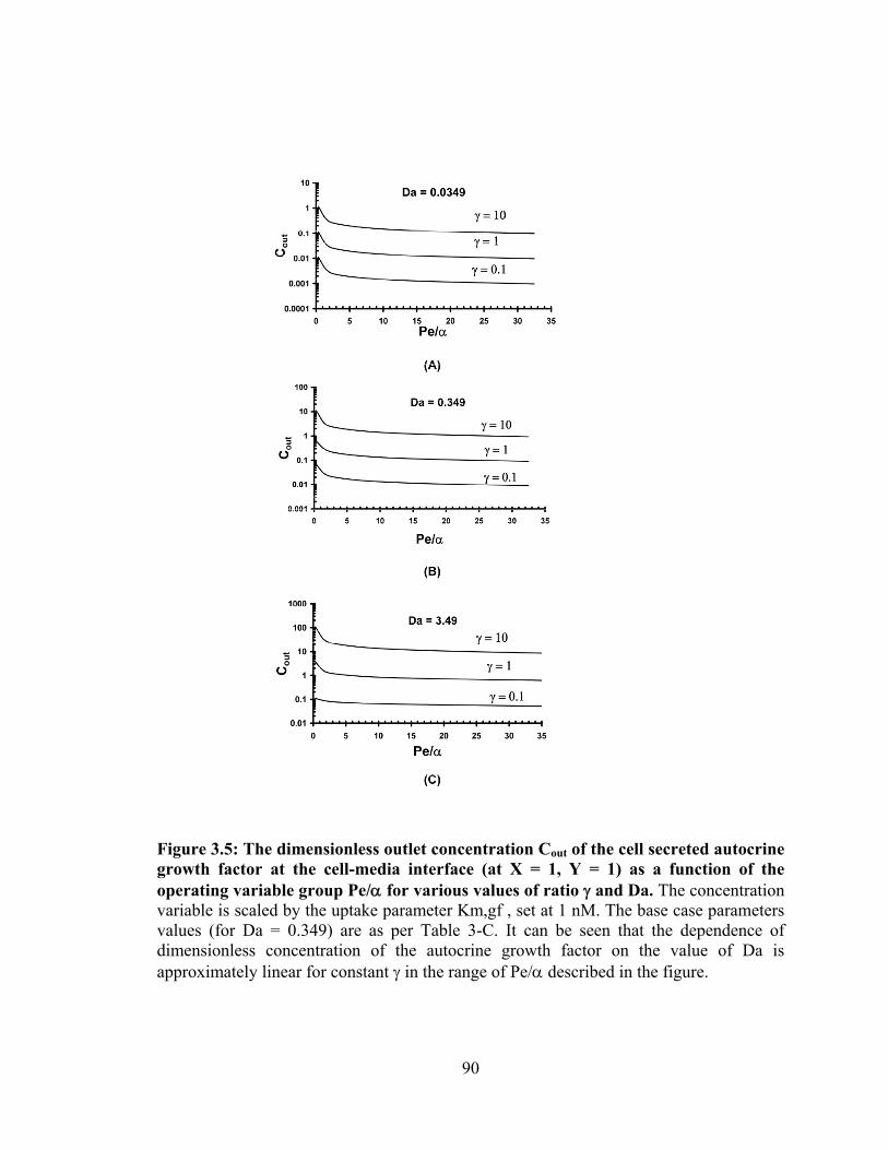
90
Figure 3.5: The dimensionless outlet concentration Cout of the cell secreted autocrine growth factor at the cell-media interface (at X = 1, Y = 1) as a function of the operating variable group Pe/α for various values of ratio γ and Da. The concentration variable is scaled by the uptake parameter Km,gf , set at 1 nM. The base case parameters values (for Da = 0.349) are as per Table 3-C. It can be seen that the dependence of dimensionless concentration of the autocrine growth factor on the value of Da is approximately linear for constant γ in the range of Pe/α described in the figure.

91
Figure 3.6: The fraction of the cell secreted autocrine growth factor lost as a function of the operating variable group Pe/α for various values of ratio γ and Da. The fraction is calculated from the results of the model using the relationship
∫
∫ ⎟⎟⎠
⎞⎜⎜⎝
⎛
= L
gf
H
x
dxq
cdyuf
0
0
φ , where the numerator is evaluated at x = L, and denominator in the cell
domain. qgf is the rate of secretion of the growth factor. The fraction lost varies over a very small range (0.95 -0.99) for values of Pe/α in the range 1.5-35 for Da = 0.0349 (not shown).
Da = 0.349
0.25
0.4
0.55
0.7
0.85
1
0 5 10 15 20 25 30 35
Pe/α
Frac
tion
Lost
, f
γ = 10
γ = 0.1
γ = 1
Da = 3.49
0.25
0.4
0.55
0.7
0.85
1
0 5 10 15 20 25 30 35
Pe/α
Frac
tion
Lost
, f
γ = 10
γ = 0.1
γ = 1

92
Figure 3.7: Effect of recirculation ratio r on the dimensionless concentration (C) of the autocrine growth (a) and nutrient concentration (b) along the dimensionless axial distance (X) at the cell media interface (Y =1). The results are shown for the base case parameters for both the nutrient and the autocrine growth factor concentrations as per Table 3-C.
(a)
00.10.20.30.40.50.60.70.80.9
1
0 0.1 0.2 0.3 0.4 0.5 0.6 0.7 0.8 0.9 1X
C
r = 0r = 0.25r = 0.5
00.10.20.30.40.50.60.70.80.9
1
0 0.1 0.2 0.3 0.4 0.5 0.6 0.7 0.8 0.9 1 X
C
r = 0r = 0.25r = 0.5
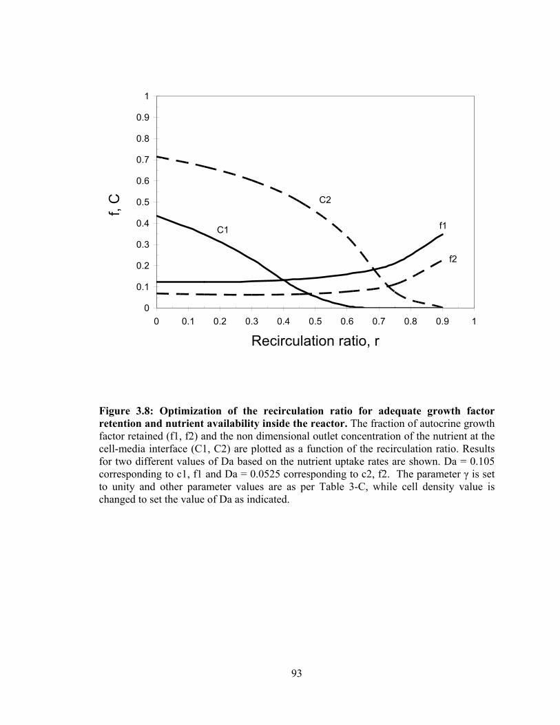
93
Figure 3.8: Optimization of the recirculation ratio for adequate growth factor retention and nutrient availability inside the reactor. The fraction of autocrine growth factor retained (f1, f2) and the non dimensional outlet concentration of the nutrient at the cell-media interface (C1, C2) are plotted as a function of the recirculation ratio. Results for two different values of Da based on the nutrient uptake rates are shown. Da = 0.105 corresponding to c1, f1 and Da = 0.0525 corresponding to c2, f2. The parameter γ is set to unity and other parameter values are as per Table 3-C, while cell density value is changed to set the value of Da as indicated.
0
0.1
0.2
0.3
0.4
0.5
0.6
0.7
0.8
0.9
1
0 0.1 0.2 0.3 0.4 0.5 0.6 0.7 0.8 0.9 1
Recirculation ratio, r
f, C C2
f1C1
f2

94
Figure 3.9: Effect of nutrient gradients on the cell density distribution inside the bioreactor. We show the impact of nutrient gradients using two example cases; case-1 (solid lines) with significant axial gradients, and case-2 (broken lines) with negligible depletion of the nutrient. The dimensionless concentration of nutrient at the cell-media interface along the non dimensional axial distance of the reactor is shown in figure (a), for various times (τ = 6, 12, 15) for both the cases. (b) shows the time evolution of cell density as a function of the non dimensional axial distance of reactor. Initially the cell density is assumed to be uniform (Φ = 1). Cell growth, reactor operation, and nutrient uptake parameters are as per Table 3-C.
0
0.1
0.2
0.3
0.4
0.5
0.6
0.7
0.8
0.9
1
0 0.1 0.2 0.3 0.4 0.5 0.6 0.7 0.8 0.9 1X
Dim
ensi
onle
ss o
utle
t con
cent
ratio
n (C
out)
Increasing τIncreasing
τ
(A)
(B)
0
1
2
3
4
5
6
7
8
9
10
0 0.1 0.2 0.3 0.4 0.5 0.6 0.7 0.8 0.9 1X
Dim
ensi
onle
ss c
ell d
ensi
ty Φ
τ = 0
τ = 6
τ = 6
τ = 12
τ = 15τ = 15
τ = 12

95
Figure 3.10: Effect of cell heterogeneity on the proliferation of cell co-culture of two cell types, with doubling times of td1=16 and td2=32 hours and with dimensionless bioreactor carrying capacity (Φ1 + Φ2)max= 10. (a) Both, the composition of the cell population represented by Φ2/Φ1 and the total cell density (Φ2 + Φ1) are shown as a function of dimensionless time τ ( = t/td1) for two different initial conditions. The cell density shown is averaged over the length of the reactor. Broken lines represent the dynamics of the culture starting at initial composition of by Φ2/Φ1=1, which also is the target composition (shown as the line Φ2/Φ1 = 1 in the figure). Solid lines are model results starting with an initial composition as estimated by model based on the doubling times. (Φ2=0.15, Φ1=0.85). (b) Dimensionless outlet concentration of the nutrient species at the cell-media interface for both the initial conditions. The maximum carrying capacity of the reactor by space considerations is 10 times the initial cell density and signifies confluence shown as the line Φ1+ Φ2 = 10 in the figure. The uptake parameters for the two cell types are Vmax,1= 1.9e-16 mol/s/cell, Vmax,2 = 9.5 e-17 mol/s/cell. The other parameters are as per Table 3-C.
0
1
2
3
4
5
6
0 3 6 9 12 15Dimensionless time, τ
Mea
n ce
ll de
nsity
ratio
( Φ2/ Φ
1)0
1
2
3
4
5
6
7
8
9
10
11
Mea
n to
tal c
ell d
ensi
ty
( Φ1+
Φ2)
Φ1 + Φ2 = 10
Φ2/Φ1 = 1
0
0.1
0.2
0.3
0.4
0.5
0.6
0.7
0.8
0.9
1
0 3 6 9 12 15
Dimensionless time, τ
Dim
ensi
onle
ss o
utle
t co
ncen
trat
ion
(Cou
t)
(A)
(B)
96
0.5. References
• Allen JW, Bhatia SN. 2003. Formation of Steady-State Oxygen Gradients In Vitro. Biotechnology and Bioengineering, 82(3):253-262.
• Allen JW, Khetani SR, Bhatia SN. 2005. In vitro zonation and toxicity in a hepatocyte bioreactor. Toxicol Sci 84(1):110-9.
• Andersson H, van den Berg A. 2004. Microfabrication and microfluidics for tissue engineering: state of the art and future opportunities. Lab Chip 4(2):98-103.
Bhalla US, Iyengar R. 1999. Emergent properties of networks of biological signaling pathways. Science 283: 381-387
• Ben-Abraham R, Gazit V, Vofsi O, Ben-Shlomo I, Reznick AZ, Katz Y. 2003. Beta-phenylpyruvate and glucose uptake in isolated mouse soleus muscle and cultured C2C12 muscle cells. J Cell Biochem 90(5):957-63.
• Botchwey EA, Dupree MA, Pollack SR, Levine EM, Laurencin CT. 2003. Tissue engineered bone: Measurement of nutrient transport in three-dimensional matrices. Journal of biomedical materials research 67A(1):357-367.
• da Silva CL, Goncalves R, Lemos F, Lemos MA, Zanjani ED, Almeida-Porada G, Cabral JM. 2003. Modelling of ex vivo expansion/maintenance of hematopoietic stem cells. Bioprocess Biosyst Eng 25(6):365-9.
• Galban CJ, Locke BR. 1999. Effects of spatial variation of cells and nutrient and product concentrations coupled with product inhibition on cell growth in a polymer scaffold. Biotechnol Bioeng 64(6):633-43.
• Ghanem A, Shuler ML. 2000. Characterization of a perfusion reactor utilizing mammalian cells on microcarrier beads. Biotechnol Prog 16(3):471-9.
• Gu W, Zhu X, Futai N, Cho BS, Takayama S. 2004. Computerized microfluidic cell culture using elastomeric channels and Braille displays. Proc Natl Acad Sci U S A 101(45):15861-6.
• Guarino RD, Dike LE, Haq TA, Rowley JA, Pitner JB, Timmins MR. 2004. Method for determining oxygen consumption rates of static cultures from microplate measurements of pericellular dissolved oxygen concentration. Biotechnol Bioeng 86(7):775-87.
• Horner M, Miller WM, Ottino JM, Papoutsakis ET. 1998. Transport in a Grooved Perfusion Flat-Bed Bioreactor for Cell Therapy Applications. Biotechnology Progress 14:689-698.

97
• Jorjani P, Ozturk SS. 1999. Effects of cell density and temperature on oxygen consumption rate for different mammalian cell lines. Biotechnol Bioeng 64(3):349-56.
• Koller MR, Emerson SG, Palsson BO. 1993. Large-scale expansion of human stem and progenitor cells from bone marrow mononuclear cells in continuous perfusion cultures. Blood 82(2):378-84.
• Koller MR, Manchel I, Palsson BO. 1997. Importance of parenchymal:stromal cell ratio for the ex vivo reconstitution of human hematopoiesis. Stem Cells 15(4):305-13.
• Lauffenburger D, Cozens C. 1989. Regulation of mammalian cell growth by autocrine growth factors: Analysis of consequences for inoculum cell density effects. Biotechnology and Bioengineering 33(11):1365-1378.
• Lauffenburger DA, Linderman JJ. 1993. Receptors: Models for Binding, Trafficking, and Signalling. Oxford University Press, Oxford.
• Leclerc E, Sakai Y, Fujii T. 2004. Microfluidic PDMS (polydimethylsiloxane) bioreactor for large-scale culture of hepatocytes. Biotechnol Prog 20(3):750-5.
• E.Leclerc, B.David, L.Griscom, B.Lepioufle, T.Fujii, P.Layrolle, C.Legallaisa. 2006. Study of osteoblastic cells in a microfluidic environment. Biomaterials 27(4):586-95
• Locker M, Kellermann O, Boucquey M, Khun H, Huerre M, Poliard A. 2004. Paracrine and autocrine signals promoting full chondrogenic differentiation of a mesoblastic cell line. J Bone Miner Res 19(1):100-10.
• Netti PA FT, Jain RK, 2003. Coupled macromolecular transport and gel mechanics: Poroviscoelastic approach. AIChE Journal 49(6):1580-1596
• Obradovic B, Meldon JH, Freed LE, Vunjak-Novakovic F. 2000. Glycosaminoglycan deposition in Engineered Cartilage: Experiments and Mathematical Model. AIChE Journal 46(9):1860-1871.
• Oehrtman GT, Wiley HS, Lauffenburger DA. 1998. Escape of autocrine ligands into extracellular medium: experimental test of theoretical model predictions. Biotechnol Bioeng 57(5):571-82.
• Palsson BO, Paek SH, Schwartz RM, Palsson M, Lee GM, Silver S, Emerson SG. 1993. Expansion of human bone marrow progenitor cells in a high cell density continuous perfusion system. Biotechnology (N Y) 11(3):368-72.
• Pathi P, Ma T, Locke BR. 2005. Role of nutrient supply on cell growth in bioreactor design for tissue engineering of hematopoietic cells. Biotechnol Bioeng 89(7):743-58.
• Rawadi G, Vayssiere B, Dunn F, Baron R, Roman-Roman S. 2003. BMP-2 controls

98
alkaline phosphatase expression and osteoblast mineralization by a Wnt autocrine loop. J Bone Miner Res 18(10):1842-53.
• Roy P, Baskaran H, Tilles AW, Yarmush ML, Toner M. 2001. Analysis of oxygen transport to hepatocytes in a flat-plate microchannel bioreactor. Ann Biomed Eng 29(11):947-55.
• Shvartsman SY, Wiley HS, Deen WM, Lauffenburger DA. 2001. Spatial range of autocrine signaling: modeling and computational analysis. Biophys J 81(4):1854-67.
• Wiley HS, Shvartsman SY, Lauffenburger DA. 2003. Computational modeling of the EGF-receptor system: a paradigm for systems biology. Trends Cell Biol 13(1):43-50.
• Williams KA, Saini S, Wick TM. 2002. Computational Fluid Dynamics Modeling of Steady-State Momentum and Mass Transport in a Bioreactor for Cartilage Tissue Engineering. Biotechnology Progress 18:951-963.
• Zandstra PW, Conneally E, Petzer AL, Piret JM, Eaves CJ. 1997. Cytokine manipulation of primitive human hematopoietic cell self-renewal. Proc Natl Acad Sci U S A 94(9):4698-703.

99
Chapter 4
4.Quantitative Inference of Cellular Parameters from
Microfluidic Cell Culture Systems
Chapter Summary
Microfluidic cell culture systems offer a convenient way to measure cell
biophysical parameters in conditions close to the physiological environment. In this
chapter, I demonstrate the application of a mathematical model describing the spatio-
temporal distribution of nutrient and growth factor concentrations in inferring cellular
oxygen uptake parameters from experimental measurements. I use experimental
measurements of oxygen concentrations in a poly(dimethylsiloxane) (PDMS)
microreactor culturing a human liver carcinoma cell line (HepG2) to infer quantitative
information on cellular uptake rates. Based on my model analysis, we have used a novel
microchannel design to avoid the parameter correlation problem associated with

100
simultaneous cellular uptake and diffusion of oxygen through the PDMS surface. It was
found that the cellular uptake of oxygen is dependent on the cell density and can be
modeled using a logistic equation. These results are significant not only for the
development of novel assays to quantitatively infer cell response to stimuli, but also for
the development, design, and optimization of novel in vitro systems for tissue
engineering.
4.1. Introduction
Microfluidics-based cell culture systems offer an inexpensive and attractive
option for culturing cells in conditions closer to physiological than static cultures (e.g.
small ratio of fluid volume to cell volume, fluid flow) and hence are favored for various
applications in biomedicine (Andersson and van den Berg 2004 ; Fisher and Peattie 2007
; Puleo, et al. 2007; Mehta et al.2008 ). Recent advances in microchannel cell culture
bioreactors have increased our ability to accurately characterize the microenvironment in
such systems by enabling control over the perfusion rate and measurement of molecular
concentrations in small samples. (Gu, et al. 2004 ; Situma, et al. 2006 ). These advances
have resulted in application of microfluidics-based systems to, for example, liver tissue
engineering and drug discovery (Kang, et al. 2008 ; Nahmias, et al. 2007 ; Viravaidya, et
al. 2004 ). However, the use of such systems for quantitative characterization of cellular
behavior remains limited. An inference procedure that can combine the mathematical
description (model) of processes occurring in microchannels with relevant experimental
measurements and subsequently extract quantitative information on key cellular
parameters would be of great significance in deciphering signaling pathways, optimizing

101
microfluidic devices for tissue engineering applications, and designing assays for
pharmacological applications. In this work, I focus on obtaining cellular parameters
describing oxygen uptake.
Oxygen is a metabolic and signaling molecule in cell culture systems, and the
oxygen consumption rate is an important metric to ascertain culture viability (Hynes, et
al. 2006 ). Information on the oxygen uptake rate of a cell culture is useful for designing
microchannel cell culture systems and also in development of various biomedical devices
including Bio-artificial liver (Balis, et al. 1999 ; Ostrovidov, et al. 2004 ; Park, et al.
2005). Typically, oxygen consumption rates in static cell cultures are measured by
tracking the oxygen concentration in the culture media for a regulated external oxygen
partial pressure (Foy, et al. 1994 ; Guarino, et al. 2004 ; Rotem, et al. 1992 ). The
applicability of the uptake rates measured in standard static cultures to physiological
conditions remains unknown. Recently, experimental techniques have been developed to
measure oxygen concentrations within microfluidic devices (Mehta, et al. 2007 ; Sin, et
al. 2004 ; Sud, et al. 2006 ). Mathematical models have also been constructed to analyze
the oxygen transfer and requirements for such perfusion based cell culture systems {{78
Roy,P. 2001; 77 Ghanem,A. 2000; 23 Mehta,K. 2006}}. However, there has been little
effort in using these models in their inverse form and developing quantitative inference
strategies to allow determination of cellular oxygen uptake parameters from experimental
data. Here, I demonstrate model-based inference of cellular uptake parameters; in the
future the pairing of quantitative assays with inference may allow the study of other
cellular responses.

102
Microfluidics-based cell culture systems are typically made from poly-dimethyl
siloxane (PDMS) in part due to its high oxygen permeability. However, the inference of
oxygen uptake rates from the experimental measurements in PDMS devices is made
difficult due to the intrinsic correlation of the model parameters characterizing the
diffusion of oxygen from PDMS surface and uptake of oxygen by cells. In the current
work, we have developed a simple experimental and computational procedure to
determine the oxygen uptake rate of a cellular culture in PDMS microchannels. I
demonstrate the performance of our method using measurements of oxygen uptake rate in
a PDMS microchannel culturing HepG2 liver cells.
4.2. Methods
4.2.1. Experimental Methods
Most of the the experimental work was performed in the research laboratory of
Prof. Shuichi Takayama by Dr. Geeta Mehta and her undergraduate associates. I am
including a brief description of the experimental methods for the sake of completion.
Microdevice Fabrication and Assembly
The microbioreactor was comprised of two compartments, a channel layer and a
PDMS-parylene C-PDMS membrane. The device was fabricated as previously described
(Mehta, et al. 2007 ). The microdevice design used for the experiments is shown in
Figure 4.1 and has a slanted channel connecting two parallel channels at the center of the
device. The cells are seeded in the slanted channel region, which is 200 μm high and 300
μm wide, while the remaining microchannels measure 30 μm high and 300 μm wide.
Fluid Flow by Braille Actuation

103
An array of 48 pin actuators adapted from a Braille display module (SC9, KGS,
Saitama, Japan) was used for fluid actuation(Futai, et al. 2006 ). The pin actuator module
was controlled with a computer via Universal Serial Bus (USB) through a finger-sized
stand alone custom controller circuit board (Olimex, Plovdiv, Bulgaria) (Futai, et al.
2006). The microfluidic bioreactor chip interfaces with the pin actuator module by simply
holding the chip in place such that the channels align with pins which push upward
closing the channel. The pin movements for valving and pumping were controlled with a
custom computer program written in C sharp. The average flow rates used for these
experiments were in the range of 0.09 to 31. 5 μm/sec. The flow rates were measured by
tracking 6 μm diameter fluorescent beads (Carnine, polystyrene microspheres, Molecular
Probes, Eugene, OR) using a digital CCD camera (Orca-ER, Hamamatsu Photonics,
Japan) and a fluorescence stereomicroscope (Nikon SMZ1500), as described in Mehta et
al. 2007. The image sequences were acquired at ~18 frames/sec to determine the velocity
of the microspheres at the center of the microchannels, which are representative of the
fluid velocity and were used to determine the average fluid flow rate. An entire pumping
cycle was used to measure each flow rate in order to compensate for backflow during
certain steps of a pumping cycle.
Cell culture
HepG2 cells (human hepatocellular carcinoma, ATCC, HB-8065) were cultured
in Dulbecco’s Modified Eagle’s Medium (DMEM, 11960, Gibco) with 15% Fetal bovine
serum (FBS, 10082, Gibco), 1%v/v antibiotic–antimicotic (15240, Gibco) and 1%v/v
GlutaMAX2-I Supplement (35050, Gibco) in a humidified 5% CO2 incubator.
Cell seeding in microdevices

104
Fibronectin (100 mg/ml, F2006, Sigma) was pipetted into the microdevices to
increase cell attachment and followed by a 30 minute absorption period. Media was then
introduced to the device and the chip was placed on an array of pin actuators adapted
from Braille displays for at least one hour to peristaltically pump fluid through the
channels. Cells (in DMEM) were seeded onto the chip through the cell seeding ports and
directed into the desired location by using Braille pumping and valving as previously
described (Mehta, et al. 2007 ). Cells were given 2-4 hours to attach under a no flow
condition and then the chip was perfused with media for 12-14 hours. The device was
maintained at 37 oC and 5% CO2.
Oxygen measurement
Dissolved oxygen concentration in microdevices was measured in real time using
an optics-based lifetime detection technique (Mehta, et al. 2007 ). An oxygen sensitive
dye, ruthenium tris(2,2’-dipyridyl) dichloride hexahydrate (RTDP) dissolved in the media
was excited by a blue LED in frequency domain by square waves generated by a function
generator. The emission signal was captured by a silicon PIN photodiode with
preamplifier and the data was acquired on a LabVIEW graphic user interface.
Oxygen concentration was determined at four points in the reactor as indicated in
4.1. We refer to the region where cells are cultured as section A of the channel (3 oxygen
measurement points) and the region downstream of the cell as section B (one oxygen
measurement point). Oxygen measurements made in section B are used to estimate the
mass transfer coefficient for oxygen diffusion through PDMS.
4.2.2. Mathematical model formulation

105
Figure 4.1 (C) shows the simplified rectangular geometry used for the model. As
in the previous chapter, the steady state concentration of oxygen (c) in the media in the
microchannel is described by the reaction-diffusion equation
ux∂c∂x
= De∂2c∂x 2 +
∂2c∂y 2
⎛
⎝ ⎜
⎞
⎠ ⎟
(4.1)
where De is the effective diffusivity of oxygen in the media and ux is the velocity. We
assume a low Reynolds number laminar unidirectional flow approximation, and the
velocity profile is estimated as (Bird, et al. 2001)
( )Hy
Hy
x uyu −= 16)( (4.2)
where, <u> is the average velocity, and H is the microchannel height. We restrict the
problem to two dimensions by neglecting the variation of oxygen concentration along the
width. We include the diffusive term in the direction of the flow (axial diffusion) because
we consider low media flow rates, although it can be neglected for relatively large flow
rates (<u> >> De/L). The inclusion of axial diffusion in the model improves the fit to
experimental data and is a significant addition to the previous model (Mehta and
Linderman 2006 ) as outlined in the earlier chapter.
The boundary conditions for (3.1) in Section A of the device (cell region) are

106
incyc =),0( (4.3)
0),( =∂∂ yLxc
(4.4)
FxycDe =
∂∂
− )0,( (4.5)
)(),( * cckHxycD lae −=
∂∂
− (4.6)
where cin is the inlet oxygen concentration and c* is the saturation oxygen concentration
at the solid (PDMS) – liquid (media) interface. We use a simple film model for the
diffusion process and the supply of oxygen from the top PDMS surface is modeled based
on an overall mass transfer co-efficient denoted by kla. We assume that there is negligible
diffusion from the bottom surface due to the presence of impermeable layer of parylene
C. F is the flux of oxygen (moles/m2-s) corresponding to the cellular uptake and is be
given by
φSOURF = (4.7)
where OURS is the specific oxygen uptake rate (uptake rate per cell) and φ represents the
cell density (cells/cm2)
In Section B there are no cells at the bottom of the microchannel, and hence that
boundary condition (Eqn. 3.5) is modified to the no flux condition
−De∂c∂y
(x,0) = 0 (4.8)
All other boundary and initial conditions (Eqns., 3, 4, and 6) remain as in Section A, with
the corresponding inlet concentration for section B equal to the concentration at the outlet

107
of the section A. The partial differential equation with non-linear boundary conditions
was solved using FEMLAB® (v3.3 & v3.4, COMSOL Inc), finite element-based
software. We verified the solution of the software by comparison with the analytical
solution of the simpler linear boundary condition problem.
Two possible relationships for the specific uptake rate (OURS) are considered
here. First, we consider the usual assumption that the specific uptake rate of oxygen
follows Michaelis-Menten kinetics with parameters Vmax and Km and is independent of
cell density (Jorjani and Ozturk 1999 ; Mehta and Linderman 2006 ). The total uptake
flux of oxygen for the cell culture is assumed to be a sum of the individual uptake rates,
e.g. a linear function of the total cell density φ (number of cells per unit area of the
channel bottom). This simplest relationship we consider is
⎟⎟⎠
⎞⎜⎜⎝
⎛+
=cKcV
OURm
Smax (4.9a)
We also consider the following alternative relationship. Because the uptake of
oxygen by cells is directly related to their growth and cell growth in spatially limited
conditions can be affected by the total cell density, the specific uptake rate of oxygen
may also depend on cell culture density. To describe this case, we incorporate a logistic
term to model the changes in the overall oxygen consumption based on the changes in the
growth rate via the total cell density. We hence propose a modified, cell density-
dependent specific uptake rate of oxygen as given by
⎟⎟⎠
⎞⎜⎜⎝
⎛−⎟⎟
⎠
⎞⎜⎜⎝
⎛+
=max
max 1φ
φcKcV
OURm
S (4.9b)
The parameter φmax represents the maximal cell density that can be cultured in the
reactor assuming no nutrient limitations. The inclusion of the logistic growth term was
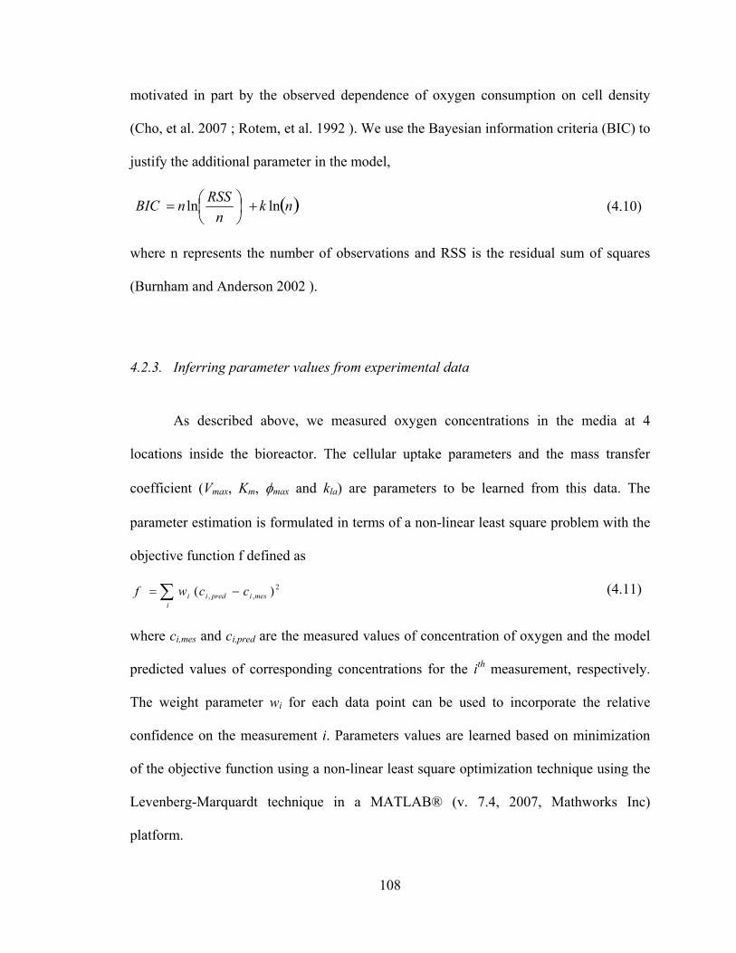
108
motivated in part by the observed dependence of oxygen consumption on cell density
(Cho, et al. 2007 ; Rotem, et al. 1992 ). We use the Bayesian information criteria (BIC) to
justify the additional parameter in the model,
( )nkn
RSSnBIC lnln +⎟⎠⎞
⎜⎝⎛= (4.10)
where n represents the number of observations and RSS is the residual sum of squares
(Burnham and Anderson 2002 ).
4.2.3. Inferring parameter values from experimental data
As described above, we measured oxygen concentrations in the media at 4
locations inside the bioreactor. The cellular uptake parameters and the mass transfer
coefficient (Vmax, Km, φmax and kla) are parameters to be learned from this data. The
parameter estimation is formulated in terms of a non-linear least square problem with the
objective function f defined as
) ( 2,, mesipredi
ii ccwf −= ∑ (4.11)
where ci,mes and ci,pred are the measured values of concentration of oxygen and the model
predicted values of corresponding concentrations for the ith measurement, respectively.
The weight parameter wi for each data point can be used to incorporate the relative
confidence on the measurement i. Parameters values are learned based on minimization
of the objective function using a non-linear least square optimization technique using the
Levenberg-Marquardt technique in a MATLAB® (v. 7.4, 2007, Mathworks Inc)
platform.

109
In principle the measurements of oxygen concentrations in section A are
sufficient to learn the parameters (Vmax, Km, φmax and kla) characterizing the system.
However, these parameters are usually highly correlated and it would require
modification of the inference procedure and a large number of measurements to learn
these parameters with a significant degree of confidence. It is hence advisable to have an
independent estimate of at least one of the two parameters Vmax and kla, as they have
highest degree of correlation. Thus we designed our reactor and experiments to allow
measurement of oxygen concentrations in a region containing no cells (section B). We
use the concentration measurements in section B of the reactor to determine kla and then
use this value and the concentration measurements in section A to learn Vmax, Km and
φmax.
The goodness of the fit was computed using the standard regression coefficient method
calculated as
∑∑
−
−−=
i
ipredi
cc
ccR 2
2,
2
)(
)(1
expi,
mesi,
(4.12)
where c is the mean experimental concentration, and the summation in Eqn. 3.11 is on
the experimental dataset under consideration. The correlation matrix (Cor) is used to
identify parameter values and its elements are computed from the covariance matrix
(Cov) given by

110
Cov=σe2(JTJ)−1 (4.13)
Cori, j =Covi, j
(Covi,iCov j , j )1/ 2 (4.14)
where n is the total number of data points (Bates and Watts 1988 ; Sadegh Zadeh, et al.
2006 ). σe is the standard deviation in the residual normalized by the total degrees of
freedom of the regression calculated as n minus the number of parameters regressed (n–
p) (Donaldson and Schnabel 1987 ).
4.2.4. Inferring confidence intervals for parameter values
The standard errors for this regression problem can be computed using the
covariance of parameters in the Cov matrix (Eqn. 3.12); however, considering that we
have errors in measurement in both dependent (c) and independent variables (chiefly <u>
and φ,), such a calculation can be inaccurate. Because the functional dependence is not
explicit, a Monte-Carlo approach should be used to compute the standard errors in
regression (Alper and Gelb 1991 ; Donaldson and Schnabel 1987 ; Motulsky and
Christopoulos 2004 ). The procedure for the simulations is followed as per Alber and
Gelb (Alper and Gelb 1991 ). New datasets are constructed by sampling the independent
variables from their individual distributions constructed from their measured variance,
and each of these datasets is used for regression to infer the parameters. The inferred set
of parameters can be used to estimate their distributions and also their confidence
intervals. Here, we sample the velocity values from a normal distribution with means and
the standard deviations estimated from our data. The value of the mass transfer
coefficient (kla) is estimated for each case using the measured oxygen concentrations in

111
section B, and subsequently the remaining parameters (Vmax, Km and/or φmax) are inferred
for each case of velocity and the kla value. The confidence interval of the inferred
parameters is reported as the standard deviations of the estimates.
4.3. Results and Discussion
4.3.1. Experimental measurements
Our experimental data on oxygen concentrations in the microdevice culturing
HepG2 cells is shown in Fig.4. 2. There is a drop in the oxygen concentration as we move
downstream, corresponding to the uptake of oxygen by cells, and this drop increases with
increasing cell density. Increasing the media flow rate (<u>) increases the overall
concentration of oxygen inside the channel as expected.
The increase in oxygen concentration in section B of the device (measurement at
x = 22.5 mm), a region in which cells are absent, provides direct evidence of the diffusive
flux of oxygen due to the permeability of the PDMS. Interestingly, the diffusion of
oxygen from the ambient air through the highly permeable PDMS devices, although
significant, is not sufficient to avoid gradients inside the microchannel.
4.3.2. Quantification of diffusion
Cells inside the microchannel are supplied oxygen by two modes – continuous
circulation of fresh media and diffusion from the ambient air via the PDMS surface.
Quantification of the specific oxygen uptake parameters (Vmax, Km and/or Φmax) by the
cells will entail the characterization of both these modes. The convective supply of

112
oxygen by the media can be calculated from the measured media flow rate and the
oxygen solubility, while the diffusion of oxygen from air is calculated based on the
estimation of the overall mass transfer coefficient kla.
The measurement of the oxygen concentration in section B (Fig. 4.2) can give an
independent estimate of the diffusive flux in the device as in that section there is no
uptake of oxygen by cells. Hence, we used the partial differential equation model and the
experimental data and formulated the optimization problem to estimate the overall mass
transfer coefficient (kla) from the experimental measurements from section B. The
agreement of the model and data is indicated in figure 4.3 and shows that the single
parameter (kla) film model of diffusive mass transfer of oxygen from PDMS surface is
sufficient to explain the diffusion process in the microdevice.
The mean value of the overall mass transfer coefficient was found to be 5.98 x 10-
8 m/s with standard deviation of 1.6 x 10⁻⁸. The standard deviation for the measurement
was estimated using the montecarlo procedure outlined earlier. Assuming normally
distributed errors in the measured variable (velocity, <u>), the fitting procedure was
repeated to estimate the standard deviation in kla and a plot of the probability distribution
of kla is shown in the inset (Fig. 4.3). We saw that the probability distribution for kla is
similar to the imposed distribution of <u>, and the measurement uncertainty of <u> is
directly reflected in the inference accuracy of kla. Interestingly, this approach can be used
to develop experimental protocols where the measurement accuracy for particular
variable is designed to achieve desired accuracy in the inferred parameter.

113
The estimated value of kla is lower than from what one would expect from virgin
PDMS, and we attribute it to the fact that the PDMS used for our experiments is plasma-
treated, which is known to lower the oxygen permeability (Houston, et al. 2002 ; Shiku,
et al. 2006 ). The dataset consists of multiple measurements with different devices and
cell cultures of different cell densities and hence the standard deviation is also indicative
of the good reproducibility of the device-making process.
4.3.3. Quantification of cellular uptake rates for experimental cell densities
We inferred the oxygen uptake rate parameters (Vmax and Km) for three different
values of cell density individually as per the uptake model described by Eqn. (3.9a) using
measured data (Fig. 4.1) from section A of the device. The goodness of the fit, as
indicated by the comparison of model and experimental results. is shown in Fig. 4.4. The
model is in good agreement of the experimental data (regression coefficients > 92%).
Table 4-A shows the inferred values of Km and Vmax for the three different cell
densities. The standard deviations in Km and Vmax for each of the three cell densities as
determined by the Monte Carlo procedure. We found that the values of Vmax vary
systematically with cell density. While the values of Km also vary for all the cell densities,
but the large standard deviations for this parameter suggests uncertainty in its values.
However, for the current experimental data, the concentrations of oxygen are much larger
than the Km values, (Km < c), and hence the specific oxygen uptake rate is largely
determined by Vmax (Eqn. 3.9a).
We found that the OURS for HepG2 cells vary between 1 x 10-17 to 9 x 10-17
mol/cell/s depending on the cell density. This rate is similar to that reported by other

114
researchers for HepG2 cell type via other measurement methods (Chin, et al. 2008 ; Liu,
et al. 1991 ). Furthermore, we found that the dependence of Vmax and hence the specific
oxygen uptake of cells on the cell density is in qualitative agreement with observations of
other researchers (Cho, et al. 2007 ; Rotem, et al. 1992 ).
4.3.4. Quantification of cellular uptake rates for unified model of oxygen uptake
The results in the previous section indicated that the specific oxygen uptake rate is
a function of cell culture density, and is lower for higher cell densities. At higher cell
densities, cells tend to grow more slowly and thus have lower metabolic activity; we
found a lower specific oxygen consumption rate. Similarly, at low cell density, when
cells tend to grow quickly and thus have a higher metabolic activity, we found higher
specific oxygen consumption. A logistic growth term, which is generally used to model
the dependence of the cell proliferation/growth rate on the instantaneous cell density,
hence should explain the dependence of our inferred cell uptake parameter on the cell
culture density. We, therefore, repeated the inference procedure with the unified model
described by Eqn. 3.9b.
The results for the fit with the new model are shown in Fig. 4.5. The inferred
values for the parameters are shown in Table 4-A. Again, as mentioned earlier, the value
of Vmax , which dominates the specific oxygen uptake rate (OURs) is in accordance with
the range of values found previously in literature, while the value of maximum cell
density Φmax is in agreement with experimentally observed maximum cell density in the
microchannel.

115
While there is an additional parameter (Φmax) for the model, we can now
simultaneously fit the data for all three cell densities (Fig. 4.5). The regression
coefficient for the new model is lower than the earlier model; however a direct
comparison of the two models is not possible by just considering the regression
coefficient, as they fit different number of datapoints, and also have different number of
parameters. Hence to verify that the additional parameter is justified, we used the
Bayesian information criterion and found the BIC score for our model (-55) is lower than
the scores of the model for three individual cell densities (-20, -27 and -25) justifying the
addition of the new parameter. The results of this analysis indicate that indeed, the
cellular uptake of oxygen is dependent on the total cell density, and hence it should be
considered while designing the oxygenation for a device meant to culture cells.
4.4. Conclusion
The motivation of this work was to develop a methodology to quantitatively
measure key cellular parameters in a specified media environment. We developed a
microfluidic device-based assay and accompanying model and inference procedure to
determine the cellular uptake rate of oxygen. By avoiding the simultaneous inference of
both the uptake and the diffusion parameters, the method used here minimizes errors
arising due to the correlation of the parameters. The independent inference of the mass
transfer coefficient is critical to the accurate inference of the cellular uptake parameters.
We also demonstrated a dependence of oxygen uptake on cell density and characterized a
new uptake model that accounts for this. Our model and associated parameter values can
be used for the design or optimization of microfluidic cell culture reactors. The method

116
and the device can be readily adapted to measure uptake rates of other soluble factors (e.g
nutrients, cell secreted signaling molecules) and also can be extended to other
systems/geometries. Furthermore, the use of model-based sensitivity studies as the Monte
Carlo simulations described here can enable the identification of variables that need to be
measured with specified accuracy to target a certain accuracy of the inferred parameter of
interest. We believe that the combination of models with new experimental devices can
help us develop novel, more accurate assays to measure the cellular properties of interest.

117
Table 4-A: Inferred parameter values and Regression Statistics4
Model - I Cell Density (φ) Vmax Km R2 BIC (x 103 cells/cm2) ( x 1017 mol/cell/s) (mol/m3)
167 1.12 [0.32]
0.12 [0.10] 95% -20
52.1 1.83 [0.57]
0.07 [0.09] 98% -27
9.9 5.74 [1.6]
0.11 [0.11] 94% -25
Model - II Cell Density Vmax Km φmax R2 BIC
(x 103 cells/cm2) ( x 1017 mol/cell/s) (mol/m3) (x 103 cells/cm2)
ALL 6.62 [1.2]
0.154 [0.087]
254 [3.4] 87% -55
4 The values inside the brackets [ ] below the reported value indicate the standard deviations in the base value ascertained by Monte Carlo simulations with 3 sets of 50 simulations each.
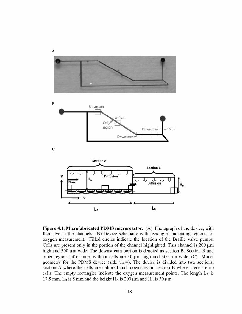
118
Figure 4.1: Microfabricated PDMS microreactor. (A) Photograph of the device, with food dye in the channels. (B) Device schematic with rectangles indicating regions for oxygen measurement. Filled circles indicate the location of the Braille valve pumps. Cells are present only in the portion of the channel highlighted. This channel is 200 μm high and 300 μm wide. The downstream portion is denoted as section B. Section B and other regions of channel without cells are 30 μm high and 300 μm wide. (C) Model geometry for the PDMS device (side view). The device is divided into two sections, section A where the cells are cultured and (downstream) section B where there are no cells. The empty rectangles indicate the oxygen measurement points. The length LA is 17.5 mm, LB is 5 mm and the height HA is 200 μm and HB is 30 μm.
A
B
y
Section A
Section B
x
HB
HA
LA LB
Flow
Diffusion
Diffusion
C

119
Figure 4.2: Oxygen concentrations in the microdevice during culture of HepG2 cells. The plots show the oxygen concentration measured in mg/L as a function of distance from the inlet. Experiments were performed at three cell densities: high (1.67 x 10⁵
cells/cm2), medium (5.2 x 10⁴ cells/cm2), and low (9.9 x 10³ cells/cm2). Four flow rates were tested and the average fluid velocity <u> is indicated. The origin or inlet is defined as the point at which the media first contacts cells as seen in Figure 4.1.

120
Figure 4.3: Determination of the mass transfer coefficient kla from oxygen concentration measurements and the model. A) shows the comparison of model and experimental data for three levels of cell density as indicated earlier. The experimentally measured scaled concentration of oxygen at the outlet of the reactor ( x = 22.5 mm ; scaled w.r.t inlet concentration) is plotted as a function of the predicted values for three cell densities circles - high (1.67 x 10⁵ cells/cm2), squares - medium (5.2 x 10⁴ cells/cm2), and stars - low (9.9 x 10³ cells/cm2). The experimental and the predicted values for all velocities are plotted with the agreement line (y=x). The best fit value for kla was 5.98 x 10⁻⁸ m/s. Three sets of 50 Monte-Carlo simulations was performed to ascertain the variation of kla for measurement uncertainty in the velocity assuming normally distributed errors with standard deviation equal to 30% of the mean. The standard deviation of the best fit kla values was found to be 1.5 x 10⁻⁸ m/s. Inset shows the cumulative probability distribution for the best fit kla values for all simulations. Note that the mean value of kla is centered, i.e has a probability of 50%. The mean regression coefficient for all the runs was 88%. All the experimental data taken in section B was used for the regression, with the inlet concentration as the concentration measured at x = 17.5 mm.

121
Figure 4.4: Comparison of predicted and observed oxygen concentrations for oxygen uptake model independent of cell density. A) Comparison of model and experimental data for three levels of cell density (circles, squares and stars for high, medium and low cell densities respectively) and for both locations (filled markers for x = 10 mm and hollow markers for x = 17.5 mm). The experimentally measured scaled concentration (scaled w.r.t inlet concentration) of oxygen at is plotted as a function of the predicted values. The experimental and the predicted values for all velocities are plotted with the agreement line (y=x). B) and C) show the comparison of the model predicted (lines) and experimental (points) scaled oxygen concentrations in the device as a function of the media velocity at locations x = 10 mm and x = 17.5 mm respectively. The experimental data in section A at three locations, x = 10 mm and x = 17.5 mm and the inlet, was used for the regression. The data for each cell density was fitted individually, hence a total of 8 points were used to infer 2 parameters. Inferred values of Vmax and Km along with the statistics for regression can be found in Table 4-A.

122
Figure 4.5: Model results with logistic growth factor densities for the proposed oxygen uptake model. A) shows the comparison of model and experimental data for three levels of cell density; High (circles), Medium (squares), and Low (stars) and for both locations (filled markers for x = 10 mm and hollow markers for x = 17.5 mm). The experimental data in section A at three locations, x = 10 mm and x = 17.5 mm and the inlet, was used for the regression. The data for all cell density was fitted simulatenously, hence a total of 32 points were used to infer 3 parameters. Inferred values of Vmax and Km along with the statistics for regression can be found in Table 4-A. B) and C) show the model (lines) and experimental results (points) as a function of the velocity for location x = 10 mm and x = 17.5 mm respectively.

123
4.5. References
Alper JS, Gelb RI. 1991. Monte Carlo method for the determination of confidence intervals: analysis of nonnormally distributed errors in sequential experiments. J Phys Chem 95:104-108.
Andersson H, van den Berg A. 2004. Microfabrication and microfluidics for tissue engineering: state of the art and future opportunities. Lab Chip 4:98-103.
Balis UJ, Behnia K, Dwarakanath B, Bhatia SN, Sullivan SJ, Yarmush ML, Toner M. 1999. Oxygen consumption characteristics of porcine hepatocytes. Metab Eng 1:49-62.
Bates DM, Watts DG. 1988. Nonlinear regression analysis and its applications. John Wiley & Sons.
Bird BR, Stewart WE, Lightfoot EN. 2001. Transport Phenomena. New York:John Wiley & Sons.
Burnham KP, Anderson DR. 2002. Model Selection and Multi-Model Inference - A Practical Information-Theoretic Approach. Springer. 488 p.
Chin K, Khattak SF, Bhatia SR, Roberts SC. 2008. Hydrogel-perfluorocarbon composite scaffold promotes oxygen transport to immobilized cells. Biotechnol Prog 24:358-366.
Cho CH, Park J, Nagrath D, Tilles AW, Berthiaume F, Toner M, Yarmush ML. 2007. Oxygen uptake rates and liver-specific functions of hepatocyte and 3T3 fibroblast co-cultures. Biotechnol Bioeng 97:188-199.
Donaldson JR, Schnabel RB. 1987. Computational Experience with Confidence Regions and Confidence Intervals for Nonlinear Least Squares. Technometrics 29:67-82.
Fisher RJ, Peattie RA. 2007. Controlling tissue microenvironments: biomimetics, transport phenomena, and reacting systems. Adv Biochem Eng Biotechnol 103:1-73.
Foy BD, Rotem A, Toner M, Tompkins RG, Yarmush ML. 1994. A device to measure the oxygen uptake rate of attached cells: importance in bioartificial organ design. Cell Transplant 3:515-527.
Futai N, Gu W, Song JW, Takayama S. 2006. Handheld recirculation system and customized media for microfluidic cell culture. Lab Chip 6:149-154.
Ghanem A, Shuler ML. 2000. Characterization of a perfusion reactor utilizing mammalian cells on microcarrier beads. Biotechnol Prog 16:471-479.

124
Gu W, Zhu X, Futai N, Cho BS, Takayama S. 2004. Computerized microfluidic cell culture using elastomeric channels and Braille displays. Proc Natl Acad Sci U S A 101:15861-15866.
Guarino RD, Dike LE, Haq TA, Rowley JA, Pitner JB, Timmins MR. 2004. Method for determining oxygen consumption rates of static cultures from microplate measurements of pericellular dissolved oxygen concentration. Biotechnol Bioeng 86:775-787.
Houston KS, Weinkauf DH, Stewart FF. 2002. Gas transport characteristics of plasma treated poly(dimethylsiloxane) and polyphosphazene membrane materials. Journal of Membrane Science 205:103-112.
Hynes J, Hill R, Papkovsky DB. 2006. The use of a fluorescence-based oxygen uptake assay in the analysis of cytotoxicity. Toxicol In Vitro 20:785-792.
Jorjani P, Ozturk SS. 1999. Effects of cell density and temperature on oxygen consumption rate for different mammalian cell lines. Biotechnol Bioeng 64:349-356.
Kang L, Chung BG, Langer R, Khademhosseini A. 2008. Microfluidics for drug discovery and development: from target selection to product lifecycle management. Drug Discov Today 13:1-13.
Liu JJ, Chen BS, Tsai TF, Wu YJ, Pang VF, Hsieh A, Hsieh JH, Chang TH. 1991. Long term and large-scale cultivation of human hepatoma Hep G2 cells in hollow fiber bioreactor. Cultivation of human hepatoma Hep G2 in hollow fiber bioreactor. Cytotechnology 5:129-139.
Mehta G, Mehta K, Sud D, Song JW, Bersano-Begey T, Futai N, Heo YS, Mycek MA, Linderman JJ, Takayama S. 2007. Quantitative measurement and control of oxygen levels in microfluidic poly(dimethylsiloxane) bioreactors during cell culture. Biomed Microdevices 9:123-134.
Mehta K, Linderman JJ. 2006. Model-based analysis and design of a microchannel reactor for tissue engineering. Biotechnol Bioeng 94:596-609.
Motulsky H, Christopoulos A. 2004. Fitting Models to Biological Data Using Linear and Nonlinear Regression. A Practical Guide to Curve Fitting. Oxford University Press. 352 p.
Nahmias Y, Berthiaume F, Yarmush ML. 2007. Integration of technologies for hepatic tissue engineering. Adv Biochem Eng Biotechnol 103:309-329.
Ostrovidov S, Jiang J, Sakai Y, Fujii T. 2004. Membrane-based PDMS microbioreactor for perfused 3D primary rat hepatocyte cultures. Biomed Microdevices 6:279-287.

125
Park J, Berthiaume F, Toner M, Yarmush ML, Tilles AW. 2005. Microfabricated grooved substrates as platforms for bioartificial liver reactors. Biotechnol Bioeng 90:632-644.
Puleo CM, Yeh HC, Wang TH. 2007. Applications of MEMS technologies in tissue engineering. Tissue Eng 13:2839-2854.
Rotem A, Toner M, Tompkins RG, Yarmush ML. 1992. Oxygen uptake rates in cultured rat hepatocytes. Biotechnol Bioeng 40:1286-1291.
Roy P, Baskaran H, Tilles AW, Yarmush ML, Toner M. 2001. Analysis of oxygen transport to hepatocytes in a flat-plate microchannel bioreactor. Ann Biomed Eng 29:947-955.
Sadegh Zadeh K, Montas HJ, Shirmohammadi A. 2006. Identification of biomolecule mass transport and binding rate parameters in living cells by inverse modeling. Theor Biol Med Model 3:36.
Shiku H, Saito T, Wu C, Yasukawa T, Yokoo M, Abe H, Matsue T, Yamada H. 2006. Oxygen Permeability of Surface-modified Poly(dimethylsiloxane) Characterized by Scanning Electrochemical Microscopy. Chem Lett 35:234-235.
Sin A, Chin KC, Jamil MF, Kostov Y, Rao G, Shuler ML. 2004. The design and fabrication of three-chamber microscale cell culture analog devices with integrated dissolved oxygen sensors. Biotechnol Prog 20:338-345.
Situma C, Hashimoto M, Soper SA. 2006. Merging microfluidics with microarray-based bioassays. Biomol Eng 23:213-231.
Sud D, Mehta G, Mehta K, Linderman J, Takayama S, Mycek MA. 2006. Optical imaging in microfluidic bioreactors enables oxygen monitoring for continuous cell culture. J Biomed Opt 11:050504.
Viravaidya K, Sin A, Shuler ML. 2004. Development of a microscale cell culture analog to probe naphthalene toxicity. Biotechnol Prog 20:316-323.

126
Chapter 5
5.A computational approach to inferring cellular protein binding
affinities from quantitative FRET imaging
Chapter Summary
Recently Fluorescence Resonance Energy Transfer (FRET) microscopy can
measure the spatial distribution of protein interactions inside live cells. Such experiments
give rise to complex data sets with many images of single cells, motivating data reduction
and abstraction. In particular, determination of the value of the equilibrium dissociation
constant (Kd) will provide a quantitative measure of protein-protein interactions that is
essential to reconstructing cellular signaling networks. In this chapter, I investigate the
feasibility of using quantitative FRET imaging of live cells to estimate the local value of
Kd for two interacting labeled molecules. An algorithm is developed to infer the values of

127
Kd using the intensity of individual voxels of three dimensional FRET microscopy
images. The performance of our algorithm is investigated using synthetic test data, both
in the absence and presence of endogenous (unlabeled) proteins. The influence of optical
blurring caused by the microscope (confocal or wide-field) and detection noise on the
accuracy of Kd inference is studied. I show that deconvolution of images followed by
analysis of intensity data at local level can improve the estimate of Kd. Finally, the
performance of this algorithm using cellular data on the interaction between YFP (yellow
fluorescent protein)-Rac and CFP (cyan fluorescent protein)-PBD in mammalian cells is
shown.
5.1. Introduction
Protein-protein interaction networks form a fundamental regulatory mechanism
controlling the behavior of living cells. Characterization of these interactions, in
particular the measurement of protein affinities, is of interest for various applications
including tissue engineering, drug discovery and development of predictive models of
cell behavior. While many methods have been developed to measure the binding
affinities of interacting proteins, including in vitro assays (Chen, et al. 2007 ; Kerppola
2006 ; Piehler 2005 ; Selbach and Mann 2006 ; Shoemaker and Panchenko 2007 ; You, et
al. 2006 ), methods for quantitative local characterization of protein-protein binding in
live cells still require improvement.
Fluorescence microscopy is the method of choice for direct visualization of
proteins in native cellular environments (Fernandez-Gonzalez, et al. 2006 ; Fricker, et al.
2006 ; Lippincott-Schwartz, et al. 2001 ; Thaler, et al. 2005 ), and recent developments in

128
imaging techniques promise measurement of protein interactions with improved spatial
and temporal resolution (Fernandez-Gonzalez, et al. 2006 ; Piehler 2005 ; Sako 2006 ).
Protein-protein binding inside live cells can be visualized by Fluorescence Resonance
Energy Transfer (FRET)(Kenworthy 2001 ). FRET is the non-radiative transfer of
fluorescence energy from an excited fluorescent donor to a nearby lower energy
fluorescent acceptor via dipole-dipole interactions. This process results in decreased
emission of the donor and increased emission from the acceptor. The range over which
FRET can occur is less than 10 nm and thus the appearance of FRET is indicative of
spatial proximity of the two interacting proteins. The spatial proximity can be used to
infer the association of donor and acceptor labeled proteins (Lakowicz 1999 ); however,
independent verification of the interaction may be required. In cellular systems, FRET
can be used to ascertain the binding of specific protein pairs by fluorescently labeling
them with different variants of fluorescent proteins. Typical experimental data in form of
large numbers of images of multiple cells make analyses difficult and time consuming.
While qualitative information on the binding affinity has been routinely inferred from the
images, methods for quantitative characterization of protein interactions are needed.
Determining the values of key physical parameters characterizing protein-protein
binding, e.g. the equilibrium dissociation constant Kd, from FRET experiments will
require additional steps beyond image acquisition. Microscope images are blurred by the
optical imaging process such that points within an image plane contain light from out-of
focus planes and adjacent points. Microscope blurring is characterized by the Point
Spread Function of the microscope (PSF), which is the image of a single point source.
This optical blurring limits the accuracy of intensity-based calculations. Confocal
129
microscopes reduce blurring as compared to conventional wide-field microscopes; but
significant optical distortion is still present. Image deconvolution algorithms can deblurr
data from both confocal and wide-field microscopes (McNally, et al. 1999 ; Swedlow
2007 ); however, their impact on the estimation of concentrations from image intensities
and hence Kd is not well understood. Further quantification of fluorescent images will
need a calibration function to map image intensities to molecular concentrations (Wu and
Pollard 2005 ). In the case of FRET microscopy, image intensities need to be corrected
for spectral overlap of the donor and acceptor emissions and possible direct excitation of
the acceptor at the donor excitation wavelength. Also, an independent estimate of FRET
efficiency (E) is needed to characterize protein binding. There are a number of algorithms
available for measurement of FRET as well as estimation of apparent FRET efficiencies
(Berney and Danuser 2003 ; Chen, et al. 2006 ; Chen and Periasamy 2006 ; Gordon, et al.
1998 ; Hoppe, et al. 2002 ; Hoppe 2007 ; Raicu, et al. 2005 ; van Rheenen, et al. 2004 ).
The presence of unlabelled proteins (endogenous, photobleached, or misfolded) which
can compete with labeled species for binding introduces an additional complication; there
have been efforts to estimate the FRET efficiency in this case (Wlodarczyk, et al. 2008 )
but the impact of such unlabelled proteins in inferring Kd remains unknown.
In this chapter, I describe my results which demonstrate the feasibility of inferring
local values of the apparent equilibrium disassociation constant (Kd) within a cell from
FRET images using a synthetic data set. I use a simultaneous image deconvolution and
spectral unmixing algorithm to accurately recover the concentration distribution of
proteins (Hoppe, et al. 2008 ) and study how the accuracy of the algorithm can aid in
estimation of local values of Kd. I investigate the impact of noise of the detection

130
systems and the presence of unlabelled (e.g. endogenous) species or multiple binding
affinities on the accuracy of Kd inference for both the wide-field microscope and also
confocal microscope. Finally, I apply this algorithm to infer Kd from image data on
binding of YFP (yellow fluorescent protein)-Rac and CFP (cyan fluorescent protein)-
PBD in mammalian cells.
5.2. Methods
5.2.1. Reaction System
We consider the case of a bimolecular elementary reaction of labeled acceptor
protein (A*) and donor-labeled protein (D*) tagged with variants of fluorescence protein
appropriate for FRET to occur:
**** DA DA ⎯⎯ →←+dK
where A*D* is the acceptor-donor complex. Binding is quantified by the equilibrium
dissociation constant (Kd) defined for a volume element v as
]D[A][D][A
**
**
=dK (5.1)
where [A*], [D*], and [A* D*] denote the concentrations of the labeled acceptor, donor
and complexes in the volume under consideration. We assume that the continuum
approximation holds within the volume, and hence Kd can be described by a mean value
rather than its probabilistic equivalent.
In a general case where there are significant amounts of unlabelled acceptor (A)
and/or donor (D) proteins present, binding reactions between labeled and unlabelled
species or between two unlabelled species can also occur:

131
A + D Kd
← → ⎯ ⎯ AD
A* + D Kd
← → ⎯ ⎯ A*D
A + D* Kd
← → ⎯ ⎯ AD*
All reactions between A and D species, whether labeled or not, are assumed to have the
same value of Kd and equilibrium relationships analogous to Eqn. (1) can be written for
each of these reactions.
5.2.2. FRET Imaging Experiment
The cell with tagged proteins is imaged using fluorescence microscopy to obtain
images with intensities corresponding to the concentrations of the acceptor, donor and
acceptor-donor complex proteins. In accordance with the nomenclature of Hoppe et al.
(Hoppe, et al. 2002 )[2], the following images of cellular contents are taken in a FRET
experiment:
IA: Image at acceptor excitation and acceptor emission (Acceptor image)
ID: Image at donor excitation and donor emission (Donor image)
IF: Image at donor excitation and acceptor emission (FRET image)
The images IA, ID and IF can be acquired on a conventional wide-field microscope or a
confocal microscope and they need to be analyzed further to gather information on the
concentrations of the individual species.
5.2.3. 3D-FRET Stoichiometry Reconstruction for Improved Local Concentration Estimates

132
We use the recently developed method termed 3D-FRET Stoichiometry (3DFSR)
to take 3D images corresponding to IA, ID and IF and, by accounting for optical blurring
due to the imaging process and donor-acceptor spectral overlap, obtain improved
estimates for the concentrations of acceptor [A*], donor [D*] and donor-acceptor complex
[A*D*] in individual 3-D image pixels (voxels). Briefly, iterative maximum likelihood
estimation is used for image deconvolution. An initial guess is convolved with the known
point spread function (PSF) of the microscope and mixed as per the spectral overlap of
donor-acceptor fluorophores to generate an estimate of the image which is then compared
with the measured image to generate the next iterate. The optimization is allowed to
proceed until a specified number (25) of iterations, the value of which is guided by our
previous work. The algorithm corrects for spectral overlap using the spectral mixing
model for FRET, which can be represented as
⎥⎥⎥
⎦
⎤
⎢⎢⎢
⎣
⎡
×⎥⎥⎥
⎦
⎤
⎢⎢⎢
⎣
⎡
−
−
=⎥⎥⎥
⎦
⎤
⎢⎢⎢
⎣
⎡
]DE[A][A][D
100
0
**tot
*tot
*
βξγξβα
γξξ
cIII
F
A
D
(5.2)
This equation relates the images (IA, ID and IF) to the concentrations of total (unbound +
bound) labeled acceptor and donor ([A*]tot and [D*]tot) and the concentration of the
acceptor-donor complex times the FRET efficiency E (E[A*D*]). In absence of any
spectral overlap, the matrix in Eqn. (2) would be an identity matrix. The constants in the
matrix are the characteristics of the microscope and fluorescent probes (Hoppe 2007 ).
The matrix operation and parameters are equivalent to FRET stoichiometry (Hoppe, et al.
2002 ), with the exception that ξ/γ as been replaced with ξ. The parameters used for our
computations are in accordance with Hoppe et al. (Hoppe 2007 )and are ξ = 0.2298, α =

133
0.025, β = 0.7275, γ = 0.0514. There are number of ways to independently estimate the
FRET efficiency with individual merits and demerits [3]. For the current work, we
assume that E is known. The factor c is the calibration constant necessary to obtain
absolute concentration values. Various approaches can be used to obtain c; however, the
estimation of c for local cellular sub compartments remains challenging (e.g. see
(Lippincott-Schwartz, et al. 2001 ), (Wu and Pollard 2005 ), (Fink, et al. 1998 )). For the
in silico imaging described here we assume that c = 1, while for the data on Rac-CFP
binding with PBD-YFP, we estimated the value of c from experiments as described
section 2.6.
5.2.4. Computing Kd from image data
For a general case when both labeled and unlabeled molecules are present, the
measured total labeled acceptor and donor concentrations include additional species:
]D[AD][A][A][A ****tot
* ++= (5.3)
]D[A][AD][D][D ****tot
* ++= (5.4)
Similarly, unlabelled total acceptor and donor concentrations can be expressed as
[AD]][AD[A][A] *tot ++= (5.5)
[AD]D][A[D][D] *tot ++= (5.6)
We define the variables rA and rD as the ratio of total labeled to unlabelled protein
concentrations for acceptor and donor inside the cell respectively:
tot
tot*
[A]][A
=Ar (5.7)

134
tot
tot*
[D]][D
=Dr (5.8)
We assume that estimates of rA and rD are available from independent population-level
experiments (e.g western blot analysis) or single cell experiments. Local values of rA and
rD within particular 3-D volume elements (voxels) can vary due to the uncertainty in the
measurement as well as fluctuations in the spatial distributions of the labeled and
unlabeled species.
Algebraic manipulation of Eqn. 4.1 (and analogous relationships with unlabeled
species) along with Eqns. 3-8 gives
( ) ( )][
][])[]([][])[]([**
**********
DArrDADAArDADADrK
DA
totDtotAd
−−−−= (5.9)
which allows a value for Kd to be calculated for each individual voxel. Individual voxel
data can be combined to generate a probability distribution of inferred Kd (normalized by
the total number of voxels in the original object) from the experimental data. The
probability that the calculated value of Kd falls within a fraction f of a given value Kd*, is
given by the area under the probability density distribution:
∫+
−
=+−∈**
**
)(]),[Pr( ****dd
dd
fKK
fKKddddddd dKKpfKKfKKK (5.10)
If the signal intensity in individual voxels is low, neighboring voxels may be binned to
form elementary volume compartments before calculation of Kd. Only those voxels (or
compartments) where both labeled proteins A* and D* are present are useful in
calculation of Kd and hence it is most efficient to perform calculations for only those

135
compartments. Furthermore, blurring redistributes light to empty voxels, resulting in
spurious estimates of Kd which are amplified by the non-linear form of Eqn. 9. Thus we
pre-select voxels for calculation of Kd based on the intensity/concentration of molecules
by using a threshold criteria to identify compartments i with useful data:
([A*],i> Γ*Max[A*]) AND ([D*]i > Γ*Max[D*]) (5.11)
Γ is the threshold parameter and defines the minimum intensity value as a fraction of the
maximum intensity value that should be present in the compartment for it to be used for
estimation of Kd. The intensity of the acceptor-donor complex is not included in the
criteria to avoid selection biases based on the value of Kd.
5.2.5. Generation of synthetic test data
We generate synthetic images to test our methods for inferring Kd. Synthetic data
generation consists of creating a cell object containing fluorescent molecules and
complexes and then simulating the imaging process by convoluting the object with the
PSF of a wide-field or confocal microscope.
First, a spherical cell object is generated using cubic 3D volume pixels (voxels).
Each voxel is randomly assigned discrete counts of labeled and unlabeled (if also present)
acceptor and donor proteins chosen from a uniform distribution over a specified interval.
The total numbers of labeled and unlabeled proteins in the object are determined from
assumed values of the ratios rA and rD. As rA and rD are parameters which can be
determined at best only on a whole cell averaged basis, for individual voxels we assume
that the ratio of labeled and unlabeled proteins is normally distributed with coefficient of
variation σr. Using these sampled values of rA and rD and the total numbers of acceptor

136
and donor proteins (A + A* and D+ D*) together with an assumed value of Kd, we
calculate the numbers of complexes (AD, A*D, AD*, A*D*) in each voxel so as to
satisfy Eqns. (3) - (8).
To simulate the imaging process, we mix the intensities on a voxel by voxel basis
to simulate spectral bleed-through, using information on the spectral overlap of CFP and
YFP to determine the mixed image as per the scheme outlined by Hoppe et al.(Hoppe et
al., 2008). In addition, we convolve this object with theoretical PSFs for either a wide-
field or confocal microscope. PSFs were generated in MATLAB 7.3 (MathWorks, Inc.,
USA) (Fig. 5.1). To simulate the spatial arrangement of multiple cells or compartments
within a single cell, images of 2 or 4 spheres with smaller radii were created. Their radii
were adjusted to keep the total volume constant. Each image is set to be equal to
100x100x100 voxels with each voxel a cube of 60 nm side.
Any imaging process with a detection device has associated inherent noise; the
presence of shot noise is unavoidable (Garini, et al. 2006 ). We simulate the shot noise in
our images by using a Poisson distributed detection noise model with variance and mean
equal to the original intensity of the object. The signal to noise ratio (SNR) is here
defined as the square root of the mean original intensity of the object, and we simulate
various noise levels by changing the intensity of the original object.
5.2.6. Live cell FRET imaging

137
The live cell image data was obtained by Dr. Adam Hoppe in the department of
microbiology and immunology at the university of Michigan. For the sake of completion
I am outlining a brief description of experimental procedure and the cell system.
COS7 cells were transfected as in (Hoppe, et al. 2008) with previously described
plasmids (Hoppe 2004) encoding YFP-Rac2(V12), CFP-PBD, CFP, YFP and YFP-CFP.
The cells with linked YFP-CFP were used as positive control, and cells expressing free
CFP and YFP molecules were used as negative control. All YFP molecules were actually
monomeric citrine, containing the Q69M (pH desensitizing) and A206K (monomeric)
mutations. PBD is the (p21 binding domain) from human PAK1. This domain provides
an excellent test system because it has been demonstrated numerous times to interact
exclusively with the small GTPases, Cdc42, Rac1 and Rac2 (Bokoch 2003 ;
DerMardirossian, et al. 2004 ).
Imaging was performed as described in (Hoppe, et al. 2008 )[4]. Briefly, a novel
high speed microscope was used to collect 3D-FRET microscopy data by acquiring IA, ID
and IF images at each z-plane of a living cell. Acquisition of each 3D dataset took
approximately 2.5 seconds. Estimates of [D*], [A*] and [DA*] were obtained by
reconstruction of these data with 3DFSR. The photobleaching correction, as estimated
from a representative experiment by the photon flux in each images IA, ID and IF
measured in successive Z-planes, was found to be less than 2% in each signal, resulting
in at the most 6% correction in the final value of Kd, and hence was neglected for the
current study.
To estimate the value of the calibration constant c, we imaged yeast cells expressing
a chromosomal YFP fusion to Arf1 (Arf1-YFP) present at 20,000 copies/cell
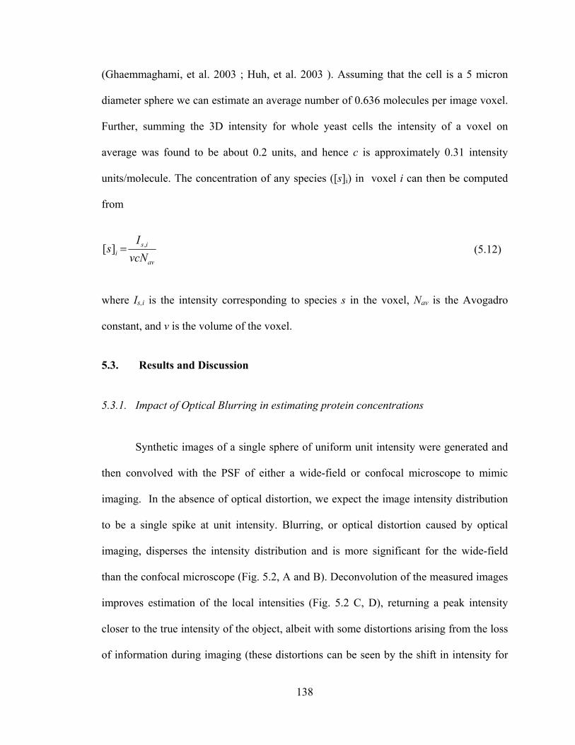
138
(Ghaemmaghami, et al. 2003 ; Huh, et al. 2003 ). Assuming that the cell is a 5 micron
diameter sphere we can estimate an average number of 0.636 molecules per image voxel.
Further, summing the 3D intensity for whole yeast cells the intensity of a voxel on
average was found to be about 0.2 units, and hence c is approximately 0.31 intensity
units/molecule. The concentration of any species ([s]i) in voxel i can then be computed
from
av
isi vcN
Is ,][ = (5.12)
where Is,i is the intensity corresponding to species s in the voxel, Nav is the Avogadro
constant, and v is the volume of the voxel.
5.3. Results and Discussion
5.3.1. Impact of Optical Blurring in estimating protein concentrations
Synthetic images of a single sphere of uniform unit intensity were generated and
then convolved with the PSF of either a wide-field or confocal microscope to mimic
imaging. In the absence of optical distortion, we expect the image intensity distribution
to be a single spike at unit intensity. Blurring, or optical distortion caused by optical
imaging, disperses the intensity distribution and is more significant for the wide-field
than the confocal microscope (Fig. 5.2, A and B). Deconvolution of the measured images
improves estimation of the local intensities (Fig. 5.2 C, D), returning a peak intensity
closer to the true intensity of the object, albeit with some distortions arising from the loss
of information during imaging (these distortions can be seen by the shift in intensity for

139
the reconstructed wide-field histogram (Fig. 5.2D) and multiple peaks in the
reconstructed confocal histogram (Fig. 5.2C)).
Recovery of true voxel intensities is also affected by the shape and spatial
arrangement of fluorophores. To investigate this, we repeated the convolution (imaging)
and deconvolution steps above with a 2 or 4 sphere arrangement (Fig. 5.1C) while
conserving the total volume of objects imaged. Fig. 5.2E shows the fraction of pixels
having intensity within 20% of the original object for the 1, 2 and 4 sphere systems.
Because spatial heterogeneity is increased, the intensity histogram is more dispersed for
multiple spheres than for a single larger sphere. This effect cannot be eliminated by
deconvolution; however, the deconvolved images are significantly more accurate than the
raw images. Deconvolution of acquired images can therefore improve the accuracy of
measurement of local molecular concentrations by estimating the true intensity of the
individual voxels. Deconvolution hence will be essential for estimation of Kd.
5.3.2. Inferring Kd from the image data
We next investigate the feasibility and accuracy of inferring Kd from measured
image data. First we considered a simple case in which all proteins under investigation
are labeled and there is no measurement noise. We assumed uniform concentrations of
acceptor, donor and acceptor-donor complex inside the 3D volume of the test object. The
test object is imaged by simulation using the 3D-FRET microscopy model (Hoppe, et al.
2008 )[4] and these images are reconstructed by 3DFSR to produce the corrected images
shown in Figs. 5.3A and 5.4A for wide-field and confocal microscopes, respectively.
Appropriate voxels were selected using the threshold criterion (Eqn. 5.11) and the

140
corresponding Kd probability distribution is calculated using Eqn. 5.9 (Figs. 5.3B and
5.4B). The fraction of voxels returning values of Kd within a specified fraction of the true
value are shown in Figs. 5.3C and 5.4C. The dispersion in the probability distribution is a
direct result of the optical distortion brought about by the imaging process. The
distributions have a maximum near the true Kd for both the confocal and the wide-field
microscopes, indicating that the proposed method is useful for identifying the local
binding affinity from image data, although optical distortion can limit its accuracy. The
effect of optical distortion on estimation of Kd increases with spatial heterogeneity (2 and
4 sphere system; Figs. 5.3 C and 5.4 C). In all cases, the confocal microscope allows
greater accuracy in measurement of Kd than the wide-field microscope.
Biological values of Kd are likely to vary widely. We repeated our inference
procedure for various values of Kd and found that the shape of the probability distribution
is unchanged. This is expected since the magnitude of intensities of the donor, acceptor,
and donor-acceptor complex images have no impact on deconvolution, and hence, in
absence of detection noise, while the absolute distortion does get scaled, the shape of the
curve does not change (data not shown).
To investigate the effect of detection noise on inference of Kd, we modeled the
image detection process with Poisson noise. The Kd probability distribution was
calculated from 3DFSR-reconstructed data with various noise levels Fig. 5.5 (A-C). As
expected, increasing noise disperses the probability distribution and limits the accuracy of
our inference. To quantify the accuracy we plot the probability of recovering the Kd
within a specified fraction of the true value (Fig. 5.5D). As shown in the figure, even at
low SNR, the algorithm can recover information on the true value of Kd.

141
5.3.3. Using thresholds to counter optical distortion and noise
Optical blurring can result in the assignment of low but non-zero intensity values
to voxels which originally have no source of fluorescence. Low voxel intensities may
also be the result of background noise. We use threshold criteria to exclude from
calculations any voxels that have intensities lower than a fraction Γ of the maximum
intensity of the acceptor and donor species in the deconvolved image data (Eqn. 11). Fig.
5.6 shows the effect of using thresholds on the Kd probability distribution for both
confocal and wide-field microscopes. Comparing the distributions obtained using
different threshold values (Fig. 5.6A, B), we can see that by limiting the calculations of
Kd to voxels/compartments with a sufficient number of acceptor and donor proteins, one
can improve the accuracy of Kd inference. This improvement is seen irrespective of the
type of microscope and also for the case with larger spatial heterogeneity (multiple
sphere system; data not shown).
Increasing the value of threshold parameter (Γ) will result in fewer compartments
used for computation, and hence the possible loss of meaningful data. On the other hand,
keeping the threshold to a lower value will result in a broader distribution owing to the
contribution of low intensity voxels. Fig. 5.6D shows the effect of increasing Γ on the
mean value of the Kd probability distribution. The results indicate that there is a
saturating effect of the threshold parameter above a critical value of the threshold. The
optimal value of the threshold parameter will depend on the microscope and cellular
system under investigation and could be found empirically e.g., by constructing the curve
similar to Fig. 5.6D.

142
5.3.4. Inferring Kd in the presence of multiple protein binding states
Multiple values of Kd for a particular protein-protein pair within a single cell may
be possible due to multiple protein states or cellular environments. To investigate the
performance of our Kd inference algorithm for such a case, we generated synthetic data
for a hypothetical case with two distinct binding constants occurring at different
concentration ratios (1:1 and 3:1) and used our algorithm to obtain the Kd probability
distribution (Fig. 5.7). To quantify the relative concentrations of each binding state, we
determined the fraction of the total voxels with a particular value of Kd. This will entail
the calculation of area under the probability distribution. However, since the spread of the
probability distribution depends on the absolute value of Kd, the correct approach is to
normalize the area under the curve by the value of Kd. Mathematically, it is equivalent to
calculating the area under the curve from a semi-log probability density distribution
A =p dKd
Kd∫ = pd log(Kd )∫ (5.13)
Fig. 5.7 shows that our algorithm can distinguish and correctly identify the
existence of the two different binding states as indicated by the two distinct peaks for
both confocal and wide-field microscopes. For the case where both the states are in equal
concentrations, the ratio of the area under the first peak to the area under the second peak
in the Kd probability distribution is 1.17 for the confocal (Fig. 5.7A) and 1.27 for the
wide-field image (Fig. 5.7B)5, reasonably close to the true value of unity. For the case
where the concentration ratios were adjusted to 3:1 in the original image, we found the
ratios of 3.22 for confocal (Fig. 5.7C) and 3.17 for wide-field image (Fig. 5.7D), again in
5 Area was computed from the semilog plot of the probability distribution with f = 0.1, 0.2 and 0.3 (see Eqn. 10) and averaging the three results for each case.

143
agreement with the true number (3.33). Thus, our algorithm can successfully identify the
relative concentrations of the two binding states. We note that the ability to distinguish
two values of Kd increases as they become more different from each other, and if they are
more spatially segregated.
5.3.5. Inferring Kd when unlabelled proteins are present
We extend our analysis to the case in which unlabelled proteins A and/or D are
present and compete with labeled species A* and D* for binding. We now need
independent measurements of the ratio of labeled to unlabelled proteins, rA and rD. (Eqns.
7 and 8), to infer binding affinity. In the limit where rA and rD are very large, there are
few unlabelled species present, and the system corresponds to the cases described in the
earlier sections.
Fig. 5.8 shows the performance of the inference procedure when unlabelled
proteins are present. A random variation of the parameters rA and rD based on a normal
distribution is superimposed to account for voxel-to-voxel variation in the number of
labeled and unlabeled molecules arising from diffusion. While the algorithm cannot
recover the true value of Kd for the case when rA and rD are small (< 0.05; data not
shown), the spread of the distribution is not affected when unlabeled proteins are present
and the distribution is similar to the case of no unlabelled species (Figs. 5.3, 5.4). Fig.
5.8 also shows the effect of these voxel-to-voxel variations on the inferred probability
distribution of Kd. Variations in parameters rA and rD will affect the accuracy of the

144
inferred Kd as per Eqn. 9, and hence we expect the probability distribution to be broader
for larger variation in rA and rD.
5.3.6. Application to cellular data on Rac-PBD binding
We applied our algorithm to FRET images obtained from imaging COS7 cells
expressing the constitutively active mutant YFP-Rac2(V12) which binds to co-expressed
CFP-PBD. Two negative controls, cells expressing free CFP and YFP-Rac2(V12) and
cells with free over-expressed CFP and YFP, were used. Linked CFP and YFP molecules
(CFP-YFP) was used as a positive control. Representative donor, acceptor, and FRET
images for all the four cases are shown in Fig. 5.9. We expect high affinity binding of
CFP-PBD with YFP-Rac2, (Fig. 5.9-A), approaching the positive control case where CFP
and YFP are linked and expressed in the cell (Fig. 5.9-D). In contrast, free CFP binds
poorly to YFP-Rac2(V12) (Fig. 5.9-B) or to free YFP (Fig. 5.9-C).
Next, we calculated Kd probability distributions from the images, neglecting
competition from unlabelled species under the assumption that the ectopically expressed
proteins were in excess. Figure 5.10 shows the computed probability distribution for all
four cases. Increasing the value of the threshold parameter Γ from 0.1 to 0.3 did not
significantly alter the location of the peak of the distribution (data not shown). We see a
single, sharp peak in the probability density distribution curve corresponding to the real
binding event of Rac-CFP with PBD-YFP (Fig 5.10A) at Kd ~ 6 μm, and a similar sharp
peak (at higher affinity) for the linked YFP and GFP case (Fig. 5.10D) at Kd ~ 1.4 μm . In
contrast, in the case of free CFP (Fig. 5.10B and C), we see a broad probability
distribution with a long tail. We attribute the small but non-zero affinity seen in the

145
negative controls (Fig. 5.10 B, C) to non-specific binding of the two molecules; the small
peak at very low affinity (Kd ~ 107μm) is partly due to the logarithmic binning used to
construct the probability distributions. We note that computational errors associated with
low intensity FRET images can make the accurate detection of low affinity binding
difficult. It is necessary to increase the number of iterations and the tolerance of the
deconvolution algorithm, as done here, to prevent the appearance of spurious peaks in the
probability distribution for the negative controls.
The probability distribution for the binding of Rac-CFP with PBD-YFP (Fig.
5.10A) can be used to compute a mean or cell-averaged value of Kd. The mean value of
Kd as measured by our algorithm is ~ 6 μM, somewhat higher than the reported in vitro
value of 0.2 μM (Hoppe 2003 ). The difference is likely at least in part real and due to
significant differences between a cellular and in vitro environment. Inaccuracies in
calibration and/or imaging and image processing may also contribute. However, our
results clearly indicate at least 3-5 orders of magnitude difference between the binding
affinities of the positive and negative control, confirming that the algorithm can identify
and also quantitatively distinguish the binding of Rac to PBD.
5.4. Conclusion
We have presented a method for inferring the local value of protein-protein
equilibrium dissociation constant Kd from FRET microscopy imaging of cells. We have
shown that deconvolution of both wide-field and confocal microscope image data is

146
essential to inferring local molecular concentrations, and hence the value of Kd, and our
algorithm can identify the existence of multiple binding states and their relative
abundance. Using synthetic test data, we show that our algorithm can provide accurate
values of Kd despite reasonable levels of noise and the presence of unlabelled proteins.
Our method builds on research done in the area of image deconvolution and
spectral unmixing for measuring FRET efficiency (Hoppe, et al. 2008 ) and the effect of
free donors and acceptors (Wlodarczyk, et al. 2008 ) by quantifying the protein
interactions via measurement of Kd. Our inference procedure utilizes the information
from small volume elements of the cell (voxels), providing a distribution probability
distribution for Kd and avoiding potential inaccuracies from averaging the signal from the
whole cell (Chen, et al. 2007 ). A key strength of our algorithm is the ability to quantify
local protein interactions, and thus it can also be applied when there is protein
sequestration or with non-cytosolic proteins. As imaging is conducted in a time frame
which is much smaller than typical protein turnover times, the algorithm will not be
affected by turnover. We have focused on intensity-based FRET measurements since they
allow measurement of [D], [A] and E[DA], which are not readily accessible by FLIM.
However, one can imagine ways in which the analysis could be extended to other types of
FRET experiments including FRET-FLIM based measurements of protein interactions
(Buranachai, et al. 2008 ; Lleres, et al. 2007 ).
The efficiency and accuracy of our approach can be affected by a number of
factors, apart from the usual parameters affecting FRET microscopy. Difficulty in
measuring the value of the calibration factor c is the primary limiting step in accurate
determination of the local value of Kd. The presence of a significant number of unlabelled

147
proteins adds the variances associated with the estimation of the local values of the ratio
parameters rA and rD to the prediction of the Kd value. Finally, our procedure involves
considerable computation as compared to the use of cell-averaging methods.
While FRET imaging is not a direct measure of the molecular interaction, it is one
of the better means of visualizing protein interactions in the native environment of the
cell and hence the ability to use FRET data to quantify the protein-protein interactions at
the subcellular scale is significant. Obtaining values of protein-protein binding affinities
may allow meaningful comparisons between the effects of different drugs or inhibitors,
giving useful insights into the mechanisms of their action. In addition, quantitative
values of protein-protein binding affinities are important for reconstructing protein
networks inside the cell. Analysis of FRET imaging data with the methods described here
might be further extended to analyze time course image data for the kinetic parameters of
protein-protein interactions.
Finally, FRET imaging can be performed with high three dimensional resolution
over time inside living cells. The terabytes of image data produced by these technologies
will far outstrip human capacity to interpret, digest, or analyze biochemical pathways.
Thus, the development of analysis tools to infer key biophysical quantities from these
image data, such as protein binding affinities described here, will be essential.

148
Figure 5.1: Point spread functions and synthetic test data. 3D Point Spread Functions (PSFs) for a wide-field (A) and confocal microscope (B) were used to generate model data. The 3D space had dimensions of 100x100x100. The x-y slice is at midplane along z (z = 50), and the x-z slice is shown at y = 50. The theoretical PSFs were generated for emission wavelength = 530 nm. NA = 1.2 and voxel size = 60x60x60 nm. Figures show color mapped images with a color map scale of [0 - 0.001] corresponding to [blue red]. (C) Synthetic spherical cells contained acceptor-donor interactions. The diameter of the single large sphere (left) was 50 pixels, equivalent to 3 µm diameter. For images containing 2 and 4 spheres, the cell diameter was adjusted to conserve total volume. The spheres were centered in z plane and were symmetrically arranged in the x-y plane.
(A)
(B)
y
x
z
x
y
x
z
x (C)
0.001
0.0
0.001
0.0

149
Figure 5.2: Deconvolution is essential for quantitative measurement of protein concentrations. The imaging process was simulated using a sphere of unit intensity and assuming a PSF for a confocal or wide-field microscope (Fig. 5.1). 3DFSR was used to deconvolve images. Confocal image and intensity histogram are shown prior to (A) and subsequent to (C) deconvolution. The intensity colormap is set to [0, 1.5] for all images for comparison. Wide-field image and intensity histogram for the intensity interval [0.1, 1.5] are shown prior to (B) and subsequent to (D) deconvolution. Solid line indicates the true intensity distribution. (E) The fraction of voxels within +/- 20% of the true value ([0.8, 1.2]) are plotted for both the confocal and wide-field microscope images, both before (blurred) and after deconvolution. The wide-field raw image before deconvolution has negligible voxels in the range, and hence don’t appear in the histogram. Results for the 2 and 4 sphere case (see Fig. 5.1) are also shown.
(A)
(C)
(B)
(D)
(E)
Confocal Widefield
z
x
y
x
z
x
y
x x
y
x
z
x
y
x
y
x
y
x
z
x
z
x
z
x
y
x
z
x
z
x
y
x
y
0.00.10.20.30.40.50.60.70.80.91.0
Deconvolved(Confocal)
Deconvolved(Widefield)
Blurred(Confocal)
Frac
tion
of p
ixel
s
124

150
Figure 5.3: Inferring Kd from wide-field image data: Effect of optical distortion. (A) Acceptor [A], donor [D], and FRET image, [DA] following imaging (convolution) by a wide-field microscope, spectral un-mixing, and deconvolution of synthetic images. The calculated Kd image is also shown. (B) The Kd probability distribution for the sphere in (A) was calculated. The solid vertical line indicates the true value of Kd and the dotted vertical lines indicates the interval +/- 10%. (C) To investigate the effect of spatial arrangement, calculations were also repeated for the 2 and 4 sphere arrangements of Fig. 5.1. The fraction of voxels with Kd within 10-40% of the true value are plotted for the 1, 2 and 4 sphere arrangements. The colormap is set to [0, 2] for all images, except the Kd image, where the colormap is set to [0, 7.5].
0.00.10.20.30.40.50.60.70.80.91.0
10% 20% 30% 40%
Frac
tion
of p
ixel
s
% of true Kd value
124
(B)
(A)
(C)
x
y
Acceptor Donor FRET
x
z
Kd
x
y
x
y
Acceptor Donor FRET
x
z
x
z
Kd

151
Figure 5.4: Inferring Kd from confocal image data: Effect of optical distortion. (A) Acceptor, donor, and FRET images following imaging (convolution) by a confocal microscope, spectral un-mixing, and deconvolution of synthetic images. The calculated Kd image is also shown. (B) The Kd probability distribution for the sphere in (A) was calculated. The solid vertical line indicates the true value of Kd and the dotted vertical lines indicates the interval +/- 10%. (C) To investigate the effect of spatial arrangement, calculations were also repeated for the 2 and 4 sphere arrangements of Fig. 5.1. The fraction of voxels with Kd within 10-40% of the true value are plotted for the 1, 2 and 4 sphere arrangements. The colormap is set to [0, 2] for all images, except the Kd image, where the colormap is set to [0, 7.5].
0.00.10.20.30.40.50.60.70.80.91.0
10% 20% 30% 40%
Frac
tion
of p
ixel
s
% of true Kd value
124
(B)
(A)
x
y
Acceptor Donor FRET
x
z
Kd
x
y
x
y
Acceptor Donor FRET
x
z
x
z
Kd
(C)

152
Figure 5.5: The effect of detection noise on inference of Kd. Poisson noise was superimposed on the convolved object to simulate detection noise. (A-C) The probability density distribution of Kd is plotted for various levels of noise: (A) SNR2 = 5, B) SNR2 = 20, C) SNR2 = 50. (D) Area under the probability density distribution curve within fraction f of the true value, where f is varied from 10% to 40%. Solid vertical lines in the plot (A-C) indicate the true value of Kd
0.0
0.2
0.4
0.6
0.8
1.0
5 10 20 50 100
Original intensity (SNR2)
Frac
tion
of v
oxel
s
10% 20%30% 40%
(D)
(A) (B) (C)

153
Figure 5.6: Using thresholding to improve Kd inference. The Kd probability distribution for confocal microscope for a single sphere was calculated using selected voxels according to a threshold criteria (Eqn. 11). Γ = 0.0 (solid line), 0.1 (dashed line) and 0.3 (dotted line) for various levels of noise: (A) SNR2 = 5 , B) SNR2 = 20, C) SNR2 = 50. ). The right portion of the curve is identical for all cases. The true Kd of the system is 5 units and is shown by the solid vertical line. (D) Calculated mean of the Kd probability distribution for various values of the threshold parameter Γ. Similar results are obtained with a wide-field microscope (not shown).
(A) (B) (C)
(D)

154
Figure 5.7: Inferring multiple values of Kd. Inferred Kd probability distributions are derived from synthetic data when the protein can bind with two possible values of Kd (Kd = 5 and Kd = 10). The 4 sphere system shown in Fig. 5.1C is used for the computations. Distributions are shown for confocal (A) and wide-field (B) microscopes with synthetic data generated so that 2 of the 4 spheres have acceptors and donors binding with affinity Kd = 5, and in the remaining 2 spheres proteins bind with affinity Kd = 10. (C) and (D) show the corresponding distributions derived from confocal and wide-field microscopes respectively, when the 3 of the 4 spheres have data corresponding to high affinity binding state (Kd = 5) and remaining 1 sphere has data corresponding to binding state Kd = 10. True values of Kd are shown by solid vertical lines.
log(Kd) log(Kd)
log(Kd) log(Kd)
(A) (B)
(C) (D)

155
Figure 5.8 : Effect of partial labeling of interacting proteins. The probability distribution of the inferred Kd is shown for rA = rD = 1. In the individual voxel the ratios were allowed to vary according to normal distribution with standard deviation 10% (A) and 30% (B). For low values of rA and rD (few labeled molecules), the algorithm will fail to recover the true values of Kd. (not shown). The figures were simulated for a confocal microscope PSF, and the true value of Kd was set at 5 units as shown by solid vertical lines.
(B)
(A)

156
Figure 5.9 : 3DFSR imaging of mammalian cells. Representative images of total donor [D*]tot, total acceptor [A*]tot and donor acceptor complex E[D*A*] after deconvolution and reconstruction from cells expressing different YFP and CFP constructs. A) Images of cell expressing YFP-Rac2(V12) and CFP-PBD. B) Images of cell expressing YFP-Rac2(V12) and free CFP (negative control). C) Images of cell expressing free CFP and free YFP (negative control). D) Images of cell expressing fused CFP-YFP (positive control). Images shown are x-y plane images at a representative z-plane and are grayscale with the same intensity map for the three images on the same row ([A*]tot, [D*A*]tot and E[D*A*]) to enable visual evaluation of binding affinity.
(A)
(B)
(C)
(D)
Acceptor Image [A*]
Donor Image [D*]
FRET image E[D*A*]

157
Figure 5.10 : Inferring Kd from 3DFSR images of mammalian cells. Inferred Kd probability distributions calculated for all four cases (Fig. 5.9A - D) are shown. A) YFP-Rac2(V12) + CFP-PBD, B) YFP-Rac2(V12) + CFP. C) YFP + CFP. D) CFP-YFP Probability distributions were constructed using a histogram method with bins of size 0.5 (μM) on the log scale. The curves shown for A) and B) are constructed from the values of 3 different experiments. The threshold value was fixed at Γ = 0.1. The mean value of Kd calculated from the distribution above based on calculations from individual pixels are 6.4 μM, 1720 μM, 129 μM and 1.19 μM, for the four cases respectively. It should be noted that the distributions for A-D are not normal, and hence the mean values are not representative of the distribution.
A) B)
D) C)

158
5.5. References
Berney C, Danuser G. 2003. FRET or no FRET: a quantitative comparison. Biophys J 84:3992-4010.
Bokoch GM. 2003. Biology of the p21-activated kinases. Annu Rev Biochem 72:743-781.
Buranachai C, Kamiyama D, Chiba A, Williams BD, Clegg RM. 2008. Rapid frequency-domain FLIM spinning disk confocal microscope: lifetime resolution, image improvement and wavelet analysis. J Fluoresc 18:929-942.
Chen H, Puhl HL,3rd, Ikeda SR. 2007. Estimating protein-protein interaction affinity in living cells using quantitative Forster resonance energy transfer measurements. J Biomed Opt 12:054011.
Chen H, Puhl HL,3rd, Koushik SV, Vogel SS, Ikeda SR. 2006. Measurement of FRET efficiency and ratio of donor to acceptor concentration in living cells. Biophys J 91:L39-41.
Chen Y, Periasamy A. 2006. Intensity range based quantitative FRET data analysis to localize protein molecules in live cell nuclei. J Fluoresc 16:95-104.
DerMardirossian C, Schnelzer A, Bokoch GM. 2004. Phosphorylation of RhoGDI by Pak1 mediates dissociation of Rac GTPase. Mol Cell 15:117-127.
Fernandez-Gonzalez R, Munoz-Barrutia A, Barcellos-Hoff MH, Ortiz-de-Solorzano C. 2006. Quantitative in vivo microscopy: the return from the 'omics'. Curr Opin Biotechnol 17:501-10.
Fink C, Morgan F, Loew LM. 1998. Intracellular fluorescent probe concentrations by confocal microscopy. Biophys J 75:1648-1658.
Fricker M, Runions J, Moore I. 2006. Quantitative fluorescence microscopy: from art to science. Annu Rev Plant Biol 57:79-107.
Garini Y, Young IT, McNamara G. 2006. Spectral imaging: principles and applications. Cytometry A 69:735-47.
Ghaemmaghami S, Huh WK, Bower K, Howson RW, Belle A, Dephoure N, O'Shea EK, Weissman JS. 2003. Global analysis of protein expression in yeast. Nature 425:737-741.

159
Gordon GW, Berry G, Liang XH, Levine B, Herman B. 1998. Quantitative fluorescence resonance energy transfer measurements using fluorescence microscopy. Biophys J 74:2702-13.
Hoppe A, Christensen K, Swanson JA. 2002. Fluorescence resonance energy transfer-based stoichiometry in living cells. Biophys J 83:3652-64.
Hoppe AD. 2003. Development of quantitative FRET microscopy for study of RHO GTPase and Phosphoninositide signaling in phagocytosis. 116 -118.
Hoppe AD, Shorte SL, Swanson JA, Heintzmann R. 2008. 3D-FRET Reconstruction Microscopy for Analysis of Dynamic Molecular Interactions in Live Cells. Biophys J 13:13.
Hoppe A. 2007. Quantitative FRET Microscopy of Live Cells. Imaging Cellular and Molecular Biological Functions. p 157-181.
Huh WK, Falvo JV, Gerke LC, Carroll AS, Howson RW, Weissman JS, O'Shea EK. 2003. Global analysis of protein localization in budding yeast. Nature 425:686-691.
Kenworthy AK. 2001. Imaging protein-protein interactions using fluorescence resonance energy transfer microscopy. Methods 24:289-96.
Kerppola TK. 2006. Complementary methods for studies of protein interactions in living cells. Nat Methods 3:969-71.
Lakowicz J. 1999. Principles of Fluorescence Spectroscopy. New York:Plenum.
Lippincott-Schwartz J, Snapp E, Kenworthy A. 2001. Studying protein dynamics in living cells. Nat Rev Mol Cell Biol 2:444-56.
Lleres D, Swift S, Lamond AI. 2007. Detecting protein-protein interactions in vivo with FRET using multiphoton fluorescence lifetime imaging microscopy (FLIM). Curr Protoc Cytom Chapter 12:Unit12.10.
McNally JG, Karpova T, Cooper J, Conchello JA. 1999. Three-dimensional imaging by deconvolution microscopy. Methods 19:373-85.
Piehler J. 2005. New methodologies for measuring protein interactions in vivo and in vitro. Curr Opin Struct Biol 15:4-14.
Raicu V, Jansma DB, Miller RJ, Friesen JD. 2005. Protein interaction quantified in vivo by spectrally resolved fluorescence resonance energy transfer. Biochem J 385:265-77.
Sako Y. 2006. Imaging single molecules in living cells for systems biology. Mol Syst Biol 2:56.

160
Selbach M, Mann M. 2006. Protein interaction screening by quantitative immunoprecipitation combined with knockdown (QUICK). Nat Methods 3:981-3.
Shoemaker BA, Panchenko AR. 2007. Deciphering protein-protein interactions. Part I. Experimental techniques and databases. PLoS Comput Biol 3:e42.
Swedlow JR. 2007. Quantitative fluorescence microscopy and image deconvolution. Methods Cell Biol 81:447-65.
Thaler C, Koushik SV, Blank PS, Vogel SS. 2005. Quantitative multiphoton spectral imaging and its use for measuring resonance energy transfer. Biophys J 89:2736-49.
van Rheenen J, Langeslag M, Jalink K. 2004. Correcting confocal acquisition to optimize imaging of fluorescence resonance energy transfer by sensitized emission. Biophys J 86:2517-29.
Wlodarczyk J, Woehler A, Kobe F, Ponimaskin E, Zeug A, Neher E. 2008. Analysis of FRET signals in the presence of free donors and acceptors. Biophys J 94:986-1000.
Wu JQ, Pollard TD. 2005. Counting cytokinesis proteins globally and locally in fission yeast. Science 310:310-4.
You X, Nguyen AW, Jabaiah A, Sheff MA, Thorn KS, Daugherty PS. 2006. Intracellular protein interaction mapping with FRET hybrids. Proc Natl Acad Sci U S A 103:18458-63.
•

161
Chapter 6
6.Conclusions and Future Directions
6.1. Summary of results
In this thesis I explored the application of computational modeling of the reaction-
diffusion systems governing the behavior of cellular systems. I have shown the utility of
my work in three distinct areas; first, microfluidics based cellular systems, second,
probing protein interactions in single cells using microscopy, and third in understanding
the mechanisms of stem cell proliferation in the context of the hematopoietic stem cell of
the bone marrow. I have applied my computational approach for both understanding the
fundamental mechanisms affecting the cellular systems and using them for novel designs,
as well as using inverse modeling to quantitatively infer properties of the cells and their
response to the microenvironment.
In chapter 2 of my thesis I have demonstrated the application of an agent based
model of adult hematopoietic system of the bone marrow. The model was formulated

162
based on the experimental observations of the hematopoietic cell behavior, and based on
the theoretical investigations I showed the relative importance of different mechanisms
which are known to play a role in the process of hematopoiesis.
In chapters 3 and 4 of the thesis I used the continuum reaction diffusion model to
characterize the microchannel devices that are preferred for culturing cells for
applications like tissue engineering and building biosensors. Using the model I identified
design criteria for developing new devices with target specifications. The model
investigated the impact of the perfusion associated ‘wash-out’ of cell secreted growth
factors and also applied the chemical engineering concept of recycle stream as a method
to retain the growth factors and outlines the optimization of recycle ratio. The model was
also investigated in its unsteady state form to arrive at useful rules of thumb governing
long-term culture of cells inside the bioreactor and also the strategy to optimize the
innoculum cell density for a specified final composition of the cells inside the bioreactor.
Next, using the inverse form of the model I outlined the method to quantitatively infer the
cellular uptake of oxygen in the culture using measurement data on oxygen concentration
in the culture. The model and the inference procedure were instrumental in identification
of dependency of the uptake rate on the cell density, and a novel model for uptake rate
was proposed.
In the penultimate chapter of my thesis, the focus was on sub cellular events,
specifically towards developing computational algorithms to infer protein binding
affinities from the live cell FRET imaging data. I showed, using the 3DFSR algorithm to
reconstruct the FRET images coupled with my computational algorithm, that the FRET
image data could be used to infer the local protein binding affinities. Further the key
163
finding of the investigation was the importance of image deconvolution in inferring the
local concentration from the fluorescence intensities, and the impact of unlabelled species
on the inferring protein binding. The feasibility of the procedure was finally showed by
analysis of preliminary image data of PBD-Rac binding in mammalian cells.
6.2. Future directions
The computational approaches used in this thesis can have potential extensions in
multiple directions within the central theme of developing quantitative tools for
biological reaction-diffusion systems. In this section I highlight a few of the natural
extensions to the work described in the thesis, and for the sake of clarity and conformity
with the division of chapters in this thesis, I classify them into three major areas. Finally I
mention some other extensions of this work in the broader area of computational biology.
6.2.1. Theoretical investigations into cell-cell interactions and the role of niche organization in adult stem cell systems
The agent based model described in chapter 2 is a novel effort to bring together
the experimental observations with varying degrees of quantification. I used it to probe
the fundamental mechanisms governing the stem cell systems. Although the model is
based on experimental observations, it is but preliminary; it does not attempt a direct
comparison with experimental results. The natural extension of the work for the adult
hematopoietic system, hence can take two directions. Firstly, the model output can be
tuned to more closely reflect the physiological system, thereby enabling model
verification using the existing experimental data. Secondly, more details can be added to

164
the model by accounting for known interactions/reactions and increasing the granularity
by explicitly accounting for different cells in the bone marrow. Recent sophisticated
experiments like e.g., the use of two photon microscopy to track the homing of the adult
human stem cells, can be used to provide useful information on the spatial dimensions
and the motility of the stem cells in the niche which can be used to accurately map the
monte-carlo time step to real time (Lo Celso, et al. 2009 ; Xie, et al. 2009 ). Addition of
the above two details would make it possible to compare the model predictions with the
experimental data in a quantitative fashion, and hence the model can be deployed in a
more predictive mode. Furthermore, the creation of such a model can be of importance in
devising in vitro systems for stem cell expansion.
The role of spatial organization in the control and regulation of hematopoietic
stem cell is but studied tacitly in the model as described in the thesis. One can think of an
equilibrium based explicit model of spatial organization of cells inside the niche upstream
of the current dynamic model to probe the role of the cellular organization in
hematopoiesis. The upstream model can be based on a modified cellular Potts model,
which has been extensively used by researchers in the chemotaxis or developmental
biology area (Chen, et al. 2007 ; Dan, et al. 2005 ; Lushnikov, et al. 2008 ). The
Hamiltonian for the cellular Potts model can be constructed using the experimentally
observed location, adhesion and proliferation behavior of the stem cells.
Another possible extension for the model is for applications involving the neural
stem cells and/or embryonic stem cells. Review of current literature on adult neural stem
cells reveals a striking similarity with the adult hematopoietic stem cell systems (Jackson,
et al. 2008 ; Jordan, et al. 2007 ; Moyse, et al. 2008). Further, the enormous therapeutic
165
potential of the embryonic stem cells and neural stem cells warrants reproducible and
robust methods for engineering these cells outside of the body to enable transplants
(Robertson, et al. 2008). The difficulty associated with experimental investigations in
such systems hence makes a strong case for development of mathematical models similar
to the ones described in this thesis which can help reduce the extensive experimentation
required to develop and optimize such stem cell engineering techniques. My work here
can be used as a good starting point, and also provides a framework from which these
models can be built .
6.2.2. Developing novel microfluidics-based devices for cell-based assays and tissue engineering
The current work has highlighted the use of models for designing and operating
microdevices for cell culture systems in from a general standpoint. Simplifying
assumptions were made to increase the applicability of the model results to most
microfluidics-based cell cultures. The ability to grow particular functional tissue systems
inside these devices, however, would require further considerations and extensions of the
model, both from the experimental as well as computational perspective.
Tissues are complex cellular systems with multiple cell types with multitude of
interactions among them, as well as with the microenvironment. Models for specific
types of tissues would require either relaxation of some of the assumptions used here, or
incorporation of newer physico-chemical mechanisms for a complete formulation. For
example, recent studies show that in developing functional bone tissue, it is known that
the flow characteristics can play a important role; the pulsatile/osciallatory nature of the
flow and the flow associated shear stress can significantly impact the growth and function
166
of the bone tissue (Du, et al. 2009a ; Du, et al. 2009b ; Jungreuthmayer, et al. 2008 ;
Kavlock and Goldstein 2008 ; Sharp, et al. 2009 ). Also, tissue engineering applications
require the use of scaffolds onto which the cells are seeded and grown. The interaction of
scaffolds with the cells adds a new dimension affecting the cell culture system
(Jungreuthmayer, et al. 2008 ; Yang, et al. 2009, Comisar, et al. 2007 ), and the
mechanisms of these interactions have to be incorporated into the model described in this
thesis. The flow pattern and shear stress can be considerably altered due to the presence
of the scaffold. While models have been developed to understand the flow and associated
stress (Maes, et al. 2009 ), such models have to be used in conjunction with the ones
described in this paper to arrive at predictive tools for building the optimal device for
bone tissue engineering. In a similar way the models and the analysis outlined in the
thesis can be extended to build novel systems for growing other functional tissues or
optimize the existing devices, e.g devices for liver tissue engineering (Altmann, et al.
2008 ; De Bartolo, et al. 2009 ; Provin, et al. 2008 ; Wen, et al. 2008 ).
The current model is built assuming a rectangular geometry of the perfusion
bioreactor. However advanced devices can have different geometries including
membrane separated ones to address specific issues of the tissue culture (e.g see
Marsano, et al. 2008 for cardiac tissue engineering; Mehta et al., 2009 for erythropoiesis
on a chip etc.) and hence another possible set of extensions to the model would be based
on relaxing the assumptions of the rectangular geometry. Further, as mentioned earlier,
the simplified laminar flow assumption would not hold with newer geometries, and hence
the model equations would have to be solved along with the equations for fluid flow.
167
Another application of the work described in the thesis involved using the inverse
form of the model to infer cellular properties. These properties can in turn be used to
characterize a more detailed model, or just to probe the fundamental behavior of the
system under consideration. In all, a new assay to quantitatively probe the cellular
function and response can be developed using a combined experimental and modeling
approach. Advances in the experimental techniques have already helped integrate
measurement techniques to dynamically monitor the cell culture in microfluidic devices,
e.g Vickerman and coworkers (Vickerman, et al. 2008 ) report a combined microfluidic
based device with real time imaging capabilities. Extending the models as described in
chapter 3-5 for such a system can enable quantifying the experimental observations.
6.2.3. Inferring biophysical parameters for cellular reactions from imaging data
The algorithm described in chapter 5 to infer sub-cellular protein binding
affinities was applied for Rac-PBD binding in mammalian cells. While we analyzed
equilibrium data for a simple bimolecular reaction, our analysis and development was by
no means restrictive, and can be easily be extended to systems with other reactions
schemes, and with multiple interacting protein pairs. Further, the analysis can be used for
time course image data to infer kinetic parameter of reactions occurring inside the cells.
A preliminary theoretical analysis of this work was done in this context for an example
system of quantifying the localization of protein in nucleus (results shown in appendix).
The next part of the work can involve extending the algorithm to infer the reaction
kinetics from the 4D image data. Such an extension can be made starting with a simpler
reaction system, and then a more detailed analysis of a small signaling pathway can be

168
done, which can be compared against available models to validate and understand our
ability to rightly model the reaction pathways inside the cell. Finally, this work can be
taken further to formulate an inverse problem strategy to infer and characterize the
reaction pathways inside the cell.
A possible extension for this project would be to use it to measure the binding
affinities of other binding systems, starting from protein-pairs that have known binding
affinities to understand the differences in the in vitro binding and the binding in cellular
environment. Further, this can be compared against a computational model to understand,
formulate, and validate the basic theory of reaction and diffusion in the cell. The model
can be developed based on the experimental system under consideration, based on any of
the excellent available models in the literature (Bhalla 2004a ; Bhalla 2004b ; Grima and
Schnell 2008 ; Wilkinson 2009 ).
Another direction to take this work to the next level would be from an
experimental perspective. As mentioned in chapter 5, calibration remains a critical step in
getting accurate quantitative information from the image data. Calibration using live cells
is a tough proposition from an experimental standpoint, as it is difficult to ascertain the
local concentrations of proteins in live cells (Wu and Pollard 2005 ), and the alternative
way of building small, microscopic entities with countable number of fluorescent
proteins is also a complicated task. Making small scale microfluidic-based designs can
be useful here as the small ‘wells’ can be etched out reproducibly in a device, and
microfluidics can be used to fill them with solutions with known concentrations of
fluorescently tagged proteins, making them ideal standards for generating calibration
data. The work done as a part of this thesis paves a way for such a system, as it can be

169
used to optimize the size and shape of the wells to give an optimal calibration system as
indicated by results in chapter 5.
6.3. Significance of current work
The work done as apart of this thesis falls under the broader, interdisciplinary
research area of computational biology. One of the major goals of the research in this
area is to fundamentally characterize the mechanisms underlying the behavior of cellular
systems and then use the knowledge to formulate a theoretical understanding. As
mentioned earlier, considering that reactions form the basic mechanisms by which the
cells communicate applications of standard chemical engineering principles to these
research problems and can offer a fresh and useful perspective.
More particularly, this thesis (Chapter 3, 4) shows how application of models
developed can reduce the time consuming and expensive experimentation required to
devise an optimal strategy to design novel systems for in vitro tissue engineering. I
believe that such a combined experimental-computational approach can be of critical
importance for generating next generation designs for growing functional biological
tissues. Furthermore, models developed in chapter 2, can help us identify and develop a
better understanding of difficult biological systems, which are not accessible from an
experimental standpoint. Similarly, the work presented in chapter 3 and 4 can be of
significance in developing next generation microfabricated systems for tissue
engineering. In chapter 5 of this thesis, I have shown the proof of concept analysis of
direct inference of protein binding affinities (Kd) from the experimental images captured
in course of FRET experiments. To the best of my knowledge, this is the first algorithm
170
attempting to quantitatively characterize the protein binding at a local, sub-cellular scale.
This work brings to light an important question: Is it possible to directly quantify the
rates of reactions occurring inside the cells from the spatio-temporal information of
molecules inside the cells? Are the reactions occurring in the cells reaction-limited, or are
they in a diffusion-controlled regime? While advances in microscopic techniques can
help us identify the spatial and temporal localization of molecules inside live cells, using
these data to characterize mathematical models of cellular signaling/reaction pathways is
not straightforward. This work, in terms of characterizing a simple equilibrium model, is
possibly the first step in answering these important questions.
The broad objective of my thesis is to develop a framework which applies
fundamental theoretical principles in conjunction with experimental observations to help
device better biomedical technologies. By developing this unified approach, I believe that
my work helps to answer existing outstanding questions in bio-chemical sciences as well
as open up newer exciting avenues of research.

171
6.4. References
Altmann B, Giselbrecht S, Weibezahn KF, Welle A, Gottwald E. 2008. The three-dimensional cultivation of the carcinoma cell line HepG2 in a perfused chip system leads to a more differentiated phenotype of the cells compared to monolayer culture. Biomed Mater 3:034120.
Bhalla US. 2004. Signaling in small subcellular volumes. I. Stochastic and diffusion effects on individual pathways. Biophys J 87:733-744.
Bhalla US. 2004. Signaling in small subcellular volumes. II. Stochastic and diffusion effects on synaptic network properties. Biophys J 87:745-753.
Chen N, Glazier JA, Izaguirre JA, Alber MS. 2007. A parallel implementation of the Cellular Potts Model for simulation of cell-based morphogenesis. Comput Phys Commun 176:670-681.
Comisar WA, Kazmers NH, Mooney DJ, Linderman JJ. 2007. Engineering RGD nanopatterned hydrogels to control preosteoblast behavior: a combined computational and experimental approach. Biomaterials 28:4409-4417.
Dan D, Mueller C, Chen K, Glazier JA. 2005. Solving the advection-diffusion equations in biological contexts using the cellular Potts model. Phys Rev E Stat Nonlin Soft Matter Phys 72:041909.
De Bartolo L, Salerno S, Curcio E, Piscioneri A, Rende M, Morelli S, Tasselli F, Bader A, Drioli E. 2009. Human hepatocyte functions in a crossed hollow fiber membrane bioreactor. Biomaterials 30:2531-2543.
Du D, Furukawa KS, Ushida T. 2009a. 3D culture of osteoblast-like cells by unidirectional or oscillatory flow for bone tissue engineering. Biotechnol Bioeng 102:1670-1678.
Du D, Furukawa KS, Ushida T. 2009b. Oscillatory perfusion culture of CaP-based tissue engineering bone with and without dexamethasone. Ann Biomed Eng 37:146-155.
Grima R, Schnell S. 2008. Modelling reaction kinetics inside cells. Essays Biochem 45:41-56.
Jackson EL, Alvarez-Buylla A. 2008. Characterization of adult neural stem cells and their relation to brain tumors. Cells Tissues Organs 188:212-224.
Jordan JD, Ma DK, Ming GL, Song H. 2007. Cellular niches for endogenous neural stem cells in the adult brain. CNS Neurol Disord Drug Targets 6:336-341.

172
Jungreuthmayer C, Donahue SW, Jaasma MJ, Al-Munajjed AA, Zanghellini J, Kelly DJ, O'Brien FJ. 2008. A Comparative Study of Shear Stresses in Collagen-Glycosaminoglycan and Calcium Phosphate Scaffolds in Bone Tissue-Engineering Bioreactors. Tissue Eng Part A
Kavlock KD, Goldstein AS. 2008. Effect of pulsatile flow on the osteogenic differentiation of bone marrow stromal cells in porous scaffolds. Biomed Sci Instrum 44:471-476.
Lo Celso C, Fleming HE, Wu JW, Zhao CX, Miake-Lye S, Fujisaki J, Cote D, Rowe DW, Lin CP, Scadden DT. 2009. Live-animal tracking of individual haematopoietic stem/progenitor cells in their niche. Nature 457:92-96.
Lushnikov PM, Chen N, Alber M. 2008. Macroscopic dynamics of biological cells interacting via chemotaxis and direct contact. Phys Rev E Stat Nonlin Soft Matter Phys 78:061904.
Maes F, Van Ransbeeck P, Van Oosterwyck H, Verdonck P. 2009. Modeling fluid flow through irregular scaffolds for perfusion bioreactors. Biotechnol Bioeng
Marsano A, Maidhof R, Tandon N, Gao J, Wang Y, Vunjak-Novakovic G. 2008. Engineering of functional contractile cardiac tissues cultured in a perfusion system. Conf Proc IEEE Eng Med Biol Soc 2008:3590-3593.
Moyse E, Segura S, Liard O, Mahaut S, Mechawar N. 2008. Microenvironmental determinants of adult neural stem cell proliferation and lineage commitment in the healthy and injured central nervous system. Curr Stem Cell Res Ther 3:163-184.
Provin C, Takano K, Sakai Y, Fujii T, Shirakashi R. 2008. A method for the design of 3D scaffolds for high-density cell attachment and determination of optimum perfusion culture conditions. J Biomech 41:1436-1449.
Robertson MJ, Gip P, Schaffer DV. 2008. Neural stem cell engineering: directed differentiation of adult and embryonic stem cells into neurons. Front Biosci 13:21-50.
Sharp LA, Lee YW, Goldstein AS. 2009. Effect of low-frequency pulsatile flow on expression of osteoblastic genes by bone marrow stromal cells. Ann Biomed Eng 37:445-453.
Vickerman V, Blundo J, Chung S, Kamm R. 2008. Design, fabrication and implementation of a novel multi-parameter control microfluidic platform for three-dimensional cell culture and real-time imaging. Lab Chip 8:1468-1477.
Wen F, Chang S, Toh YC, Arooz T, Zhuo L, Teoh SH, Yu H. 2008. Development of dual-compartment perfusion bioreactor for serial coculture of hepatocytes and stellate cells in poly(lactic-co-glycolic acid)-collagen scaffolds. J Biomed Mater Res B Appl Biomater 87:154-162.
173
Wilkinson DJ. 2009. Stochastic modelling for quantitative description of heterogeneous biological systems. Nat Rev Genet 10:122-133.
Wu JQ, Pollard TD. 2005. Counting cytokinesis proteins globally and locally in fission yeast. Science 310:310-4.
Xie Y, Yin T, Wiegraebe W, He XC, Miller D, Stark D, Perko K, Alexander R, Schwartz J, Grindley JC, Park J, Haug JS, Wunderlich JP, Li H, Zhang S, Johnson T, Feldman RA, Li L. 2009. Detection of functional haematopoietic stem cell niche using real-time imaging. Nature 457:97-101.
Yang J, Cao C, Wang W, Tong X, Shi D, Wu F, Zheng Q, Guo C, Pan Z, Gao C, Wang J. 2009. Proliferation and osteogenesis of immortalized bone marrow-derived mesenchymal stem cells in porous polylactic glycolic acid scaffolds under perfusion culture. J Biomed Mater Res A


![Reaction rates for mesoscopic reaction-diffusion … rates for mesoscopic reaction-diffusion kinetics ... function reaction dynamics (GFRD) algorithm [10–12]. ... REACTION RATES](https://img.dokumen.tips/doc/110x75/5b33d2bc7f8b9ae1108d85b3/reaction-rates-for-mesoscopic-reaction-diffusion-rates-for-mesoscopic-reaction-diffusion.jpg)