Computational modelling of left ventricular haemodynamics ... · Computational modelling of left ventricular haemodynamics based on magnetic ... Coherent vortex formation is observed

Computational modelling of left ventricular haemodynamics based on magnetic resonance imaging data

Nikoo R. Saber1 & A.D. Gosman2

1Graduate Aeronautical Laboratories, California Institute of Technology, Pasadena, CA, USA.2Department of Mechanical Engineering, Imperial College London, United Kingdom.

Abstract

A combined computational fl uid dynamics (CFD) and magnetic resonance imaging (MRI) methodology has been developed to simulate blood fl ow in a subject-specifi c left heart. The research continues from earlier experience in modelling the human left ventricle using time-varying anatomical MR scans. Breathing artefacts are reduced by means of an MR navigator echo sequence with feedback to the subject, allowing a near constant breath-hold diaphragm position. An improved interactive segmentation technique for the long- and short-axis anatomical slices is used. The computational domain is extended to include the proximal left atrium and ascending aorta as well as the left ventricle, and the mitral and aortic valve orifi ces are approximately represented. The CFD results show remarkable correspondence with the MR velocity data acquired for comparison purposes, as well as with previously published in vivo experiments (velocity and pressure). Coherent vortex formation is observed below the mitral valve, with a larger anterior vortex dominating the late diastolic phases. Some quantitative discrepancies exist between the CFD and MRI fl ow velocities, due to the limitations of the MR dataset in the valve region, heart rate differences in the anatomical and velocity acquisitions, and certain phenomena that were not simulated. The CFD results compare well with measured ranges in literature.

1 Introduction

The fl ow conditions and local blood fl ow patterns in the heart chambers are closely associated with many cardiac disorders [1]. To that end, there is an important body of work on blood fl ow within the heart [2–4]. In the past, progress in CFD modelling of cardiac haemodynamics has been impeded by a number of factors, including diffi culties in obtaining the necessary anatomical information, limitations in CFD methodology and insuffi cient computing power. These have tended to constrain the scope and realism of such studies, particularly in respect of over-idealized representation of the anatomy. This has been particularly true in the case of heart chambers, where the highly complex time-varying anatomical features make it dif-fi cult to create in vitro models which are suffi ciently similar in geometry to the real anatomy. As a consequence, research in heart modelling has been rather sparse and limited, the best focusing on simplifi ed models based on animal casts and cadavers. Very few investigators have used realistic in vivo data, for example [5]. Nonetheless, the large vessel studies to date have

WITPress_RRPS_ch003.indd 47WITPress_RRPS_ch003.indd 47 4/12/2008 3:42:39 PM4/12/2008 3:42:39 PM

www.witpress.com, ISSN 1755-8336 (on-line) WIT Transactions on State of the Art in Science and Engineering, Vol 35, © 2008 WIT Press

doi:10.2495/978-1-84564-096-5/03

48 REPAIR AND REDESIGN OF PHYSIOLOGICAL SYSTEMS

provided encouraging indications that CFD can provide more detailed qualitative and quantita-tive information about cardiovascular fl ows, leading to a better understanding [6], especially when employed in combination with MR imaging [4, 7]. Even in terms of visualization, CFD can assist conventional clinical fl ow monitoring techniques by providing additional information about the complex fl ow patterns. The understanding of these three-dimensional time-varying structures can be quite diffi cult, since the visualization modes are generally two-dimensional views of three-dimensional phenomena.

The research described here has as its objective the development of a combined CFD and MRI methodology for the simulation of patient-specifi c fl ow in the heart chambers. This is done through studies with healthy human subjects. The work thus differs from previous computational fl ow studies of the left ventricle, which have mostly been generic and idealized, or derived from animal casts, or comprised only of a specifi c portion of the cardiac cycle, e.g. fi lling [8, 9].

The present study continues from research previously reported by Saber et al. [10] with the incorporation of some important improvements. The aforementioned research built in turn on pilot studies [11, 12] involving MR geometry and fl ow measurements combined with CFD techniques; this approach has been adapted to the left ventricle in the present work. In summary, the proposed framework employed MRI scans of a human heart to obtain geometric data, which were then used for the CFD simulations. These latter were accom-plished by geometrical modelling of the ventricle using time-resolved anatomical slices of the ventricular geometry and imposition of infl ow and outfl ow conditions at orifi ces notionally representing the mitral and aortic valves. The predicted fl ow structure evolution and physiologically relevant fl ow characteristics were analysed and compared to existing information. The CFD model convincingly captured the three-dimensional contraction and expansion phases of endocardial motion in the left ventricle, allowing simulation of domi-nant fl ow features, such as the vortices and swirling structures. These results were qualita-tively consistent with previous physiological and clinical experiments on in vivo ventricular chambers, but the accuracy of the simulated velocities was limited largely by the anatomical shortcomings in the valve region. The study also indicated areas in which the methodology requires improvement and extension.

Despite being an important step in haemodynamical modelling, there were various defi cien-cies in the computational fl ow model of the left ventricle discussed by Saber et al. [10]. The use of diaphragm position gating via the post-navigator echo, in order to reduce breathing artefacts in the MR anatomy acquisition, prevented data acquisition towards the end of the pulse cycle [10, 13]. During this period, the navigator data were processed on-line, and simultaneous data acquisition was not possible. Furthermore, the level of spatial resolution prevented the detection of the valve areas, so detail in the basal region had to be approximated to an excessive degree for the model.

These shortcomings have been addressed in the new subject-specifi c model and CFD simulation. The main modifi cations are improved acquisition protocols and new segmentation methodology, allowing the inclusion of the proximal left atrium and ascending aorta, linked to the ventricle by better-defi ned valve regions. Whilst the details of the valve leafl ets still could not be resolved, good representations of the valve ring locations, morphology and motion were obtained, allowing more realistic representation of this region than in the previous study. The anatomy was determined using MRI as before and then represented by a body-fi tted moving mesh, including representation of the valve orifi ces, for the numerical solution of the Navier-Stokes fl ow equations [10].

Additionally, MR velocity images from the subject modelled were acquired in the oblique long-axis plane containing both valves. Comparisons have been made with these measurements and with published velocity and pressure data for the left ventricle.



COMPUTATIONAL MODELLING OF LEFT VENTRICULAR HAEMODYNAMICS 49

2 Methods

Magnetic resonance images of the left ventricle of a 26-year-old healthy female volunteer were acquired on a 1.5 Tesla MR scanner system (EDGE Powerdrive 250, Picker International Inc., Cleveland, OH), as used in our earlier study [10].

Preliminary short-axis pilot acquisitions located the plane passing through the mitral and aortic valves. This allowed location and acquisition of the oblique long-axis plane of the left ventricle, orthogonal to the above short-axis plane and passing through the mitral valve, apex and aortic valve [2]. Moreover, vertical and horizontal long-axis planes were acquired. A set of short-axis planes was acquired, parallel to the pilot short axis, in ten contiguous slices from above the top basal plane to the apex, ensuring that the main body of the left ventricle was entirely captured, and allowing inclusion of part of the left atrium and the ascending aorta. As before [10], the ventricular chamber itself was captured by either seven or eight of the total of the fi xed SA slice locations, depending on the phase. Figure 1 shows an image of the oblique long-axis plane seen as from below, with the subject’s posterior towards top left hand (LH) corner, left aspect towards lower LH corner. The endocardium is outlined, showing the apex at the bottom of the outline and the base at the top, with the ascending aorta to the right and left atrium to the left of the view.

Figure 1: Oblique long axis MR image plane through the subject’s heart, seen from below. Poste-rior aspect is towards upper left of image; anterior towards lower right. Manually traced outline indicates computational domain comprising left ventricle (LV) and proximal left atrium (LA) and ascending aorta (AA). LA is at top left of outline; AA is at top right (Reproduced from [14] with kind permission of Springer Science and Business Media).




The anatomical acquisitions employed for the determination of the ventricle geometry models were cardiac-gated (triggered from the R-wave of the ECG), using a cine segmented FLASH (Fast Low Angle SHot) sequence (TE 3.8 ms; inter-frame interval 35.6 ms; RF fl ip angle 25 deg; slice thickness 10 mm; FOV 400 mm2; in-plane resolution 1.56 mm). Gating delays for short- and long-axis acquisitions were identical. The post-navigator echo [13] was used to monitor the diaphragm position and respiration phase. Additional gating was then applied to accept data from only a narrow range of diaphragm positions, hence minimising respiratory motion artefacts in the image acquisition. However, on-line implementation of this on the Picker Edge scanner required a period of approximately 300 ms at the end of each ECG-gated cycle, during which image data could not be acquired, resulting in loss of important functional information [10]. To overcome this problem, the cine frames were triggered only every other cardiac cycle, allowing a complete set of frames to be acquired during the fi rst of successive pairs of cycles. In addition, a methodology combining breath holding with the navi-gator echoes was employed, incorporating verbal feedback to the subject being scanned. With this technique, the images could be acquired over multiple reproducible breath-holds. A total of 24 phases was acquired over two cycles in this manner, of which 16 covered one cardiac cycle with a period of 569.6 ms.

Velocity scans were acquired via the phase velocity mapping technique in the oblique long-axis plane, encoded in all three gradient directions (velocity window 200 cm/s for each component). MR velocity errors were expected to be within 5–10% of the window setting [11]. The velocity images, also acquired with the use of both the navigator and breath holding, were gated from the R-wave of the ECG. Once again, 16 phases were acquired to cover one cardiac cycle, but the subject’s average R-R interval had increased from 569.6 ms in the anatomical scan to 649.6 ms during the velocity scans, probably owing to different states of wakefulness.

2.1 Data processing and geometry reconstruction

A new semi-automatic technique, devised and incorporated in the CMRTools© suite, allowed a complete reconstruction of a left ventricle model, incorporating also proximal regions of the left atrium and ascending aorta [15]. Short- and long-axis images were displayed simultaneously, so segmentation in the two planes proceeded interactively, reducing registration errors [16]. For each phase, each control point on the endocardium was constrained to lie on the intersec-tions of the short- and long-axis views. Therefore, information from two images could be used simultaneously when placing each control point, and the post-segmentation reconciliation used previously [10] was not required. Short-axis slices provide good resolution through ‘infl ow enhancement’, since blood moves at a signifi cant rate perpendicular to the imaging plane, intro-ducing fresh signal and resulting in high-defi nition images. By contrast, long-axis slices tend to have low infl ow enhancement but suffer little from partial volume effects; thus, combining the two different slice orientations gave an improved segmented image.

The number of control points that could be determined from these data for each phase was insuffi cient to defi ne the ventricle geometry completely. Therefore, additional long-axis planes were reconstructed by fi tting further B-spline curves to the short-axis images; their planes lay perpendicular to the short-axis images, with radial orientations chosen to place them at regular intervals between the measured planes. These long-axis images benefi ted from the signifi cantly greater contrast between blood and endocardium in the short-axis images, as discussed above. This more comprehensive set of curves lying in the endocardial surface allowed the addition or manipulation of control points to obtain the desired boundary locations.




2.2 CFD methodology and computer code

The fl ow simulations were performed using the fi nite volume (FV) method [17], as imple-mented in the STAR-CD code (Computational Dynamics Ltd., London, UK), and fully described elsewhere [10]. Briefl y, the FV method used in the code solves the full Navier–Stokes equations by an effi cient implicit time-marching procedure, which allows the use of structured or unstruc-tured, body-fi tted moving meshes within the time-varying geometry.

2.3 Generation of computational mesh

Once the endocardial control point data had been extracted from the MR images, B-spline surfaces were fi tted to the points. Additional modifi cation was then required to smooth the union of the main ventricle volume with the infl ow and outfl ow tract domains, which could be attached to the main ventricular domain as part of the meshing procedure. Separate lay-ered multiblock hexahedral grids were fi tted to each of the three modelled sub-volumes for each phase, using an automated parametric procedure especially developed for this purpose, described and illustrated by Saber et al. [10]. Then, the atrial and aortic meshes were con-nected to the main ventricle mesh by the ’arbitrary interfacing’ feature of the code, which permits dissimilar meshes to be joined at a common interface, at which sliding may occur. The latter fl exibility greatly facilitated the calculation of the mesh motion, described below. The meshes at each of the odd-numbered measured phases, 1, 3, 5,…, 15, are shown in Figure 2.

Phase 7

Phase 15

Phase 5

Phase 13

Phase 3

Phase 11

Phase 1

Phase 9

Figure 2: Computational meshes formed for the odd-numbered measured phases in a cycle. Phases 1–7 systole; phases 9–15 diastole (Reproduced from [14] with kind permission of Springer Science and Business Media).




2.4 Wall and mesh motion

Further computational meshes were required at intermediate times between consecutive measured phases of the cardiac cycle, and were obtained by interpolating between the initial meshes created. It was necessary to specify the motion of the ventricle wall and mesh between the measurement phases. An assumed mode of movement of surface points was imposed, in which each point travelled inwards or outwards along a ray of fi xed angular position emanating from the centroid of the slice containing it [10].

Instead of the linear temporal interpolation scheme used previously [10], a second-order scheme, comprising piecewise quadratic ‘blending’, was developed [18]. This allowed continu-ous value and gradient interpolation for all three coordinate directions, the ‘values’ being the positions of the vertices and the ‘gradients’ their velocities. Thus, separate meshes were deve-loped for each of the 1600 time-steps required for each cycle in order to satisfy the Courant criterion [17] (see Section 2.6).

2.5 Boundary conditions

Since the anatomical short-axis slices extended beyond the ventricle base and included the infl ow and outfl ow tracts, the simulation domain included the mitral and aortic valves, but there was insuffi cient detail to show the exact locations of the valve rings. Moreover, no modelling of the valve leafl ets could be attempted, since the scans also did not provide this level of detail. Opening and closing orifi ces (‘pseudo valves’) were therefore set at the two basal boundaries to the domain, in the infl ow and outfl ow tracts (Figure 2). Each ‘pseudo-valve’ orifi ce was made to open and close instantaneously at the start and end of the appropriate phase of the cardiac cycle, marked by the change in sign in the rate of total volume change. A relative pressure boundary condition was set at whichever ‘pseudo-valve’ plane was open. This allowed the computation of pressure variations within the domain, relative to the boundary value. The relative pressure differences, which relate to the local velocity variations, may be compared with multi-sensor catheter measurements [19, 20].

The measured time-varying volume of the computational domain (Figure 3) allows the computation of volume rate of change. Since the FV solution method enforces overall mass conservation at each time step, this determines instantaneous volume fl ow rate in and out of the modelled region through the basal openings, and the instantaneous average infl ow and outfl ow velocities through these openings, dividing the volume fl ow rates by the cross-section areas. No through-plane instantaneous velocity distributions were acquired which could be used as velocity boundary conditions, so they were calculated from the uniform boundary pres-sure assumption and the internal pressure fi eld [10]. Independently of this, there were three reasons for the imposition of pressure boundary conditions instead of measured velocities: (1) the change of heart rate between the anatomy and velocity determinations; (2) the limited accuracy of the latter; (3) the movement of the ventricle (and mesh) relative to the fi xed measurement planes, precluding direct determination of the velocities on the inlet plane of the calculation.

The positions of the minimum areas in the mitral and aortic tracts approximated to the valve ring positions. For the simulations in this study, the mitral annulus area was slightly reduced from the outline obtained in the segmentation by the incorporation of a 1 mm rim at the junc-tion between the infl ow tract and ventricle, like an orifi ce plate, formed by impermeable cell surfaces, termed ‘baffl es’. This had the effect, like the valve leafl ets, of confi ning the infl ow jet and allowing space for the diastolic posterior vortex to develop in a realistic fashion.




In their measurements of the velocity through the mitral valve during late diastole, Kim et al. [2] noted velocity magnitudes at the mitral valve leafl et tips about 19% greater than that at the mitral annulus, owing to the contraction in cross-section. Fujimoto et al. [21] measured a similar increase of 15–20% in their MR measurements. The presence of the baffl es described above, in addition to confi ning the jet through the valve ring, was also expected to create a vena contracta downstream from the mitral ring and hence approximate the effects of the leafl ets just described.

Despite the various remaining shortcomings, the new model represents a signifi cant advance on our earlier one [10]. It appears from our results, shown later, that the details currently mod-elled allow adequate simulation of the main fl ow features, with some peripheral inaccuracies.

2.6 Flow simulation procedure

Blood was assumed to be a homogeneous Newtonian fl uid with a dynamic viscosity approxi-mated as 4×10−3 Pa.s. and a density of 1050 kg/m3. The simulations commenced from an ini-tially quiescent fl ow state and were continued for a number of full cardiac cycles in order to allow development of a fully periodic fl ow, representative of a regular heartbeat. It was found that the main features of the internal fl ow fi eld became repeatable within 4 cycles, but the slow end-diastolic vortical motions required 6 cycles to reach a repetitive state. Aspects of this are discussed in the next subsection and in the Results and Discussion sections.

The results reported here were obtained on a mesh with 90 layers, each comprising 500 cells, in the main body of the ventricle. In each of the tracts, 22 layers of 500 cells were used, resulting in a total of 67,000 cells in the entire computational domain. This produced adequate spatial resolu-tion (see below) when the second-order ‘MARS’ discretisation scheme [22] in the code was used. The size of the computational timestep was set at a value of 0.356 ms, hence maintaining the value of the Courant number in the simulations (the product of the timestep with the ratio of the local fl uid velocity and mesh spacing) to less than unity over most of the computational domain [17].

0 8 16 24 32Phase Number

4e-05

5e-05

6e-05

7e-05

8e-05

9e-05

0.0001

0.00011

Vol

ume

[m3 ]

MRIQuadratic interpolation

Systole Diastole

Figure 3: Variation of volume of computational mesh with phase number (time) (Reproduced from [14] with kind permission of Springer Science and Business Media).




2.7 Mesh and timestep sensitivity

Sensitivity tests showed that the total number of cells in the ventricular model and the chosen computational timesteps were suitable for the results to be grid- and timestep-independent to an acceptable level of tolerance. When the total number of cells was increased by a fac-tor of 1.533 = 3.375 to 226125, (50% decrease in the cell dimensions) and the timestep was decreased by a factor of 1.5 to 0.237 ms (to maintain cell Courant numbers below unity [17]), the fl ow maintained its overall structure in the ventricle model. The volume-averaged velocity in the fi ne mesh remained within 2% of the value for the coarser mesh, although the mass fl ow rate through the open valves differed by a maximum of 6–8% between the two cases in peak systole and peak diastole. The differences observed, however, resulted mainly from better fi tting of the mesh to the computational domain boundaries rather than better resolution of the discretized fl ow equations. Since the fi ner mesh conforms better to the boundaries, it occupies more volume, but given the MR measurement uncertainties, the associated computation time penalty was considered unjustifi ed.

3 Results

3.1 Cardiac output and ejection fraction

Figure 3 shows the modelled domain volume versus time variation for two cardiac cycles. The points indicate the measurement phases, and the lines are the quadratic interpolations. The instants of simulated valve opening and closure (at minimum and maximum volume: phases 7 and 16, respectively) are indicated in the plot. The increased rate of change at phase 14 (t = 462.8 ms) is probably related to atrial systole. The volume of the modelled ventricle is 59 ml at end-systole and 104 ml at end-diastole, giving a stroke volume of 45 ml. The end values are towards the upper limit of the normal range previously measured in females [23], but the ejection fraction was low at 43.3%; normal values are 53.9–75.6% [24]. This low ejec-tion fraction appears to be compensated by the high heart rate of the subject (about 105 beats per minute), giving a cardiac output of 4.725 l/min. The observed volumes are boosted by the inclusion of the papillary muscles within the apparent LV lumen, since they could not be resolved adequately by the MR images.

3.2 Quantitative comparison of calculated and measured fl ow fi elds

As already noted, the MR velocity scans in this study were acquired at a slower heart rate, and therefore with a larger interframe interval, compared with the anatomical scans. In both the fl ow and anatomical scans, one complete cardiac cycle was captured in 16 phases, but changes in heart rate are usually accompanied by changes in the relative lengths of systole and diastole as well as velocity changes [25]. Nevertheless, each acquired velocity phase appears to correspond with the equivalent anatomical phase (from which the simulations were derived) throughout the cardiac cycle. Our comparison of the CFD velocity results and the MR fl ow maps is based on this approximate correspondence.

Figure 4(a)–(e) contains the comparisons of the oblique long-axis views, containing both valve locations, with the MR velocity images on the left and the CFD results on the right, showing the main phases of systole (1–4) and diastole (9–14). The smaller diagram below each simulation indicates the phase on a plot of the volume variation. The view is as from




Figure 4: Vectors of simulated velocities (right-hand side) in the time-varying oblique long-axis plane compared with MR velocity vectors in the same plane (left-hand side). Views are as from above left, with the subject’s anterior aspect to the left and the subject’s left towards the bottom of the views. The velocity vector scale is constant through the MR plots, but in the simulations changes between systole and diastole. The smaller diagram below each simulation indicates the phase on a plot of the volume variation. Figure 4(a): phases 1–2; Figure 4(b): phases 3–4 (systole). Figure 4(c): phases 9–10; Figure 4(d): phases 11–12; Figure 4(e): phases 13–14 (diastole) (Reproduced from [14] with kind permission of Springer Science and Business Media).

(b)

0.5 m/s

(c)

1 m/s 1 m/s

(a)




above left, with the subject’s anterior aspect to the left of the views and the subject’s left towards the bottom. The endocardial outline derived from the anatomical scans is superim-posed on the measured vectors for comparison with the simulations. There are high-velocity vectors outside the ventricular region in the MR measurements, showing fl ow in neighbouring vessels or, in the upper RHS (right-hand side) of the fi gures, high noise levels in the low signal returned by lung tissue. Figure 5 shows diastolic short-axis views of the simulated fi elds, which will be commented on later.

The scale of the MR velocity vectors is the same for all phases and is indicated on Figure 4(a) (phase 1), whilst the scales of the simulation vectors are larger in diastole (scale arrows in Figure 4(a) (phase 1) and Figure 4(c) (phase 9)). The qualitative comparisons discussed below show good correspondence between the simulated and the measured fl ow structures. The dif-ferences in the heart rate during the acquisition of the MR anatomical and velocity data inhibit a straightforward quantitative comparison between the CFD and MRI fl ow results; moreover, the comparison is infl uenced differently in systole and diastole.

At peak systole the measured velocity was 1.25 m/s compared with 1.57 m/s simulated. A possible rationale may be given for this comparison. If both the cardiac output and the stroke volume were largely unchanged when the heart rate changed, the velocities might then be in approximately the inverse ratios of the cycle periods. The faster rate of change of ventricular

Figure 4: Continued

(e)

(d)




volume measured at the faster pulse rate correctly gives rise to higher velocities. The measured endocardial outlines match well with the velocity images when superimposed (Figure 4), giving some support for assuming the stroke volume was relatively unchanged. The ratio of cycle periods was 1.14 compared with a peak velocity ratio of 1.26, so the hypothesis is only weakly confi rmed. In fact, the cardiac outputs would not be identical in the two experiments, since differing degrees of wakefulness would require differing levels of cerebral fl ow.

At peak diastole the measured velocity magnitude at the level of the mitral ring was approxi-mately 0.50 m/s, fairly uniform across the jet, compared with 0.42 m/s in the simulation. The measured velocity in the jet was boosted by the reduced effective mitral ring area, resulting from the fl ow separation induced by the left inferior pulmonary vein fl ow, which enters the atrium near the mitral entrance (see Section 4). The mitral ring area itself is known to change during the cycle; it also descends and rises. This anatomical variation was measured and included in the model. The boosted peak MR velocity image levels in diastole suggest that the separation-induced reduction in effective mitral ring area had a greater effect than that of the change in pulse rate, reversing the direction of change seen in systole.

The typical velocity measurement uncertainty is 5% of the 200 cm/s window setting, i.e. 10 cm/s, a substantial fraction of the highest diastolic velocities. Therefore, when the velocity levels in the ventricular domain are small, the MR velocity uncertainties are comparable to the actual velocities. The accuracy of the simulated fl ow structure is directly affected by the accu-racy of the MR anatomical data and the derived wall motion.

Phase 13 Phase 14

Phase 15 Phase 16

Figure 5: Vectors of simulated diastolic velocities in a short-axis plane near the base for phases 13–16. The velocity scales are different for each of the phases; maximum velocities are phase 13: 0.30 m/s; phase 14: 0.30 m/s; phase 15: 0.30 m/s; phase 16: 0.23 m/s (Repro-duced from [14] with kind permission of Springer Science and Business Media).




4 Discussion

The simulated long-axis fl ow patterns of the model ventricle are closely similar in topology to the MR measurements in Figure 4(a)-(e) as well as to measurements by Kim et al. [2], notably during early diastolic fi lling, when the fl ow structure shows most detail.

The MRI and CFD results for systole (phases 1–4, Figure 4(a) and 4(b)) are generally similar except at phase 1, when the MR velocity images show both valves closed. For the later systolic phases of the cycle (peak-systole is at phase 3, Figure 4(b)), both sets of results show the fl ow converging towards the outfl ow tract with similar overall patterns. In the CFD model, it was required that at least one fl ow boundary was open at any given time during the simulations, in order to satisfy continuity in the incompressible fl ow, since the modelled volume rate of change was always non-zero. The accuracy of geometry determination from MR anatomy images did not allow identifi cation of periods of constant volume, when concurrent closure of both valves would have been possible.

In early diastole, both the CFD and MRI velocity plots show the fl ow entering the ventricle as a short plug of high-velocity fl uid (phase 10, Figure 4(c)), similar to the structure observed by Lemmon and Yoganathan [26] in their idealized numerical model of the left ventricle diastolic phase. The fl ow fi lls the infl ow orifi ce in the simulation and is fairly uniform entering the ventricle, but the open aortic root allows local fl ow development in a limited region. In the MR image for phase 10, when the incoming fl ow jet is displaced from the posterior wall of the main body of the ventricle, it attaches to the anterior wall, but by phase 11 (Figure 4(d)) it has separated again. Kim et al. [2] observed a similar phenomenon in their measurements: after peak diastole, the anterior mitral leafl et tip was seen to hit the septal wall (the anterior wall of the ventricle) and then retract, allowing the vortex to develop behind it, and subsequently causing the mitral infl ow vector to be angled more towards the posterior wall.

Thus, by phase 11 (Figure 4(d)) the incoming velocity profi les are skewed towards the pos-terior wall of the ventricle in both the CFD results and the MR measurements. Deeper into the ventricle, the fl ow in the CFD results is more directed towards this wall and less towards the apex. Both the anterior and posterior vortices below the mitral ring have started to form in both plots, but MR and CFD are not completely in phase. In the MR plots, a stream may be seen entering the atrium from the inferior left pulmonary vein; this causes a fl ow separation at the mitral ring, which persists into the ventricle and may infl uence the posterior vortex.

At phases 12 and 13 (Figure 4(d) and (e)), the separation induced by the pulmonary vein continues in the MR images, affecting the fl ow in the ventricle. The two diastolic mitral vortices have stabilized in both the CFD and the MR fl ow fi elds, with good correspondence. A similar recirculation pattern, beneath the leafl ets of the mitral valves, has been reported previously by Kim et al. [2] and Kilner et al. [27]. Phase 14, Figure 4(e), appears to represent the start of atrial contraction as mentioned earlier. The incoming fl ow jets in the MR images do not extend as far as the simulations along the longitudinal axis of the ventricle, but it should be recalled that the papillary muscles are not represented within the simulated ventricular lumen, distorting the apical geometry. The anterior vortex in both the MR measurements and the CFD simulations appears to be located just beneath the supposed position of the anterior leafl et of the mitral valve (phases 13 and 14 in Figure 4(e)), and the correspondence between the main vortical structures in MR and simulated fl ows is particularly notable in these phases.

Kilner et al. [27], in their study of a number of normal subjects, observed a transient vortex beneath the region of the posterior mitral valve leafl et, once again similar to our simulated results. Their observation of velocity components in a long-axis plane led them to believe that diastolic secondary fl ow might have the character of an asymmetric annular vortex. The present




simulated fl ow results in short-axis planes (Figure 5) show a dominant anterior vortex and a smaller-scale posterior vortex, but do not give clear indication of a contiguous annular vortex surrounding the jet.

4.1 Comparison with other data

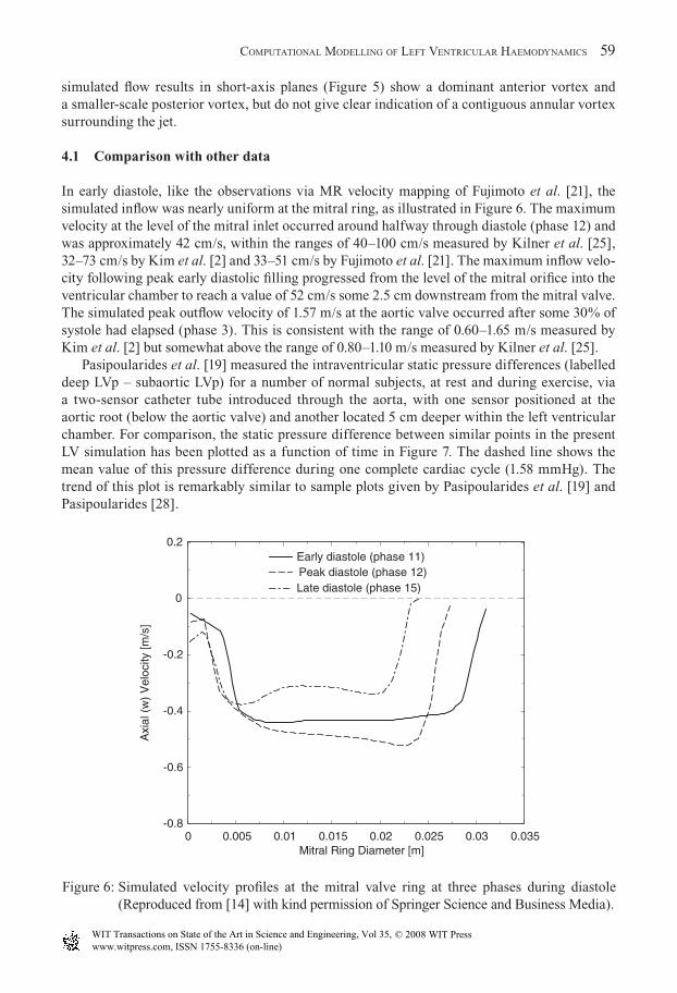
In early diastole, like the observations via MR velocity mapping of Fujimoto et al. [21], the simulated infl ow was nearly uniform at the mitral ring, as illustrated in Figure 6. The maximum velocity at the level of the mitral inlet occurred around halfway through diastole (phase 12) and was approximately 42 cm/s, within the ranges of 40–100 cm/s measured by Kilner et al. [25], 32–73 cm/s by Kim et al. [2] and 33–51 cm/s by Fujimoto et al. [21]. The maximum infl ow velo-city following peak early diastolic fi lling progressed from the level of the mitral orifi ce into the ventricular chamber to reach a value of 52 cm/s some 2.5 cm downstream from the mitral valve. The simulated peak outfl ow velocity of 1.57 m/s at the aortic valve occurred after some 30% of systole had elapsed (phase 3). This is consistent with the range of 0.60–1.65 m/s measured by Kim et al. [2] but somewhat above the range of 0.80–1.10 m/s measured by Kilner et al. [25].

Pasipoularides et al. [19] measured the intraventricular static pressure differences (labelled deep LVp – subaortic LVp) for a number of normal subjects, at rest and during exercise, via a two-sensor catheter tube introduced through the aorta, with one sensor positioned at the aortic root (below the aortic valve) and another located 5 cm deeper within the left ventricular chamber. For comparison, the static pressure difference between similar points in the present LV simulation has been plotted as a function of time in Figure 7. The dashed line shows the mean value of this pressure difference during one complete cardiac cycle (1.58 mmHg). The trend of this plot is remarkably similar to sample plots given by Pasipoularides et al. [19] and Pasipoularides [28].

0 0.005 0.01 0.015 0.02 0.025 0.03 0.035Mitral Ring Diameter [m]

-0.8

-0.6

-0.4

-0.2

0

0.2

Axi

al (

w)

Vel

ocity

[m/s

]

Early diastole (phase 11)Peak diastole (phase 12)Late diastole (phase 15)

Figure 6: Simulated velocity profi les at the mitral valve ring at three phases during diastole (Re produced from [14] with kind permission of Springer Science and Business Media).




At peak systole, the simulated peak positive pressure difference is about 9.3 mmHg, slightly outside the SD (standard deviation) of Pasipoularides’s measurements of 6.7 ± 1.9 (SD) mmHg at rest. This result is obviously infl uenced by the fast heart rate and high systolic velocities of the subject scanned for the present study. It was closer to submaximal exercise, in which Pasipoularides et al. [19] measured 10.0 ± 1.8 mmHg. During late systole, as the ejected fl ow retards, the simulations show the expected negative pressure difference between the two sensor locations with a peak value of -2 mmHg. During the early diastolic portion of the car-diac cycle, the pressure difference again becomes negative as the ventricular volume expands, subsequently declining towards zero. During late diastole, the pressure difference becomes positive as the incoming fl ow retards.

These intraventricular pressure differences are consistent with studies via cardiac cath-eterisation conducted not only by Pasipoularides [28] but by Smiseth et al. [20], and via CFD modelling by Georgiadis et al. [29]. They are related to the inertial resistance of blood to temporal and convective acceleration [12].

4.2 Physiological plausibility and signifi cance of fl ow predictions

It has been suggested by Kim et al. [2] that the motion of the mitral valve leafl ets promotes the development of ventricular vortices, as observed in their MR velocity maps. However, despite the absence of leafl et modelling in our simulations, the typical vortices were evident in the domain. Similarity of infl ow patterns between the CFD model and velocity images in this study and those quoted in literature suggests that the structure of the valve leafl ets is not essential for the genera-tion of these vortices. Clearly, it relates to the vorticity in the valve region, which is induced by the shear between the jet and the surrounding fl uid. The diastolic vortices have been attributed a

1 3 5 7 9 11 13 15Phase Number

-4

-2

0

2

4

6

8

10

∆P [m

m H

g]

Figure 7: Temporal variation of the simulated pressure difference between the aortic valve and a point located 5 cm deeper into the left ventricle (LV), representing the pressure difference recorded by a two-sensor catheter introduced into the LV via the aorta (Reproduced from [14] with kind permission of Springer Science and Business Media).




benefi cial role in terms of energy preservation and have been suggested to infl uence mitral valve motion [2], although Reul et al. [30] showed that they were unnecessary to the valve closure process. During exercise, when diastole is shorter, the dominant recirculation under the anterior leafl et appears to assist the redirection of infl owing blood towards the outfl ow tract [27].

By end-systole, much of the swirling motion in the computed fl ow has subsided and the outfl ow is almost unidirectional with fl ow converging towards the left ventricular outfl ow tract from the entire ventricular chamber. This is in line with expectations, as well as observations by Kim et al. [2]. The velocity distribution in the aortic annulus in normal subjects has been found to be slightly skewed [31]. The most likely explanation for this profi le is thought to be the position and angulation of the left ventricular outfl ow tract relative to the chamber [2]. Close observation of the velocity plots during late systole (Figure 4(c)) also shows a skew with higher velocity towards the anterior aspect.

4.3 Potential clinical applications

There are clinical implications for any deviation of the fl ow structure from that observed and measured. For example, in normal healthy subjects, cine velocity mapping has shown that the predominant direction of diastolic fl ow through the mitral valve is towards the apex during diastolic fi lling, and converging from the apex to fl ow out through the aortic valve in systole [32], similar to the fl ow simulation results of the present study. However, in patients with a severely dilated left ventricle (resulting from coronary heart disease), Mohiaddin’s MR velocity mapping [32] showed that the infl ow is directed not towards the apex, but towards the posterior wall, giving rise to a well-developed circular fl ow pattern turning back towards the septum and outfl ow tract and persisting through diastole to the next systolic phase. Some authors have used simple models to simulate these effects [10], but clearly the ability to represent them more accu-rately as with the present method has advantages, including the potential to perform ‘virtual surgery’, as explored in other areas of cardiovascular fl ow research [33].

5 Conclusions

A framework has been developed for the simulation of fl ow in the heart chambers and demon-strated by application to the left ventricle. The methodology relies on MR anatomical data and surface fi tting techniques to construct a dynamic geometrical model of the chamber anatomy, which is then fi tted with a moving mesh for CFD simulations by a semi-automatic parametric procedure. It also allows for future refi nement of the boundary conditions, by introducing valve leafl ets at the mitral orifi ce and extending the computational domain.

Computational fl ow simulations were conducted for a left ventricle model incorporating the infl ow (mitral) and outfl ow (aortic) tracts. The fl ow structure and its evolution were analysed in the numerical results and compared with existing measurements of physiologically relevant parameters. The model convincingly captured the 3D contraction and expansion phases of endocardial motion in the left ventricle. The time-varying volume of the model produced a physiologically plausible stroke volume and ejection fraction. The analysis also revealed that the dominant fl ow features from the simulations were qualitatively and quantitatively consistent with previous physiological and clinical experiments, as well as with velocity measurements acquired with the anatomical data for the present study.

Coherent vortex formation was observed immediately below the mitral valve, with a pair of counter-rotating vortices occurring during left ventricular diastole. Owing to heart rate differences




in the MR anatomical and velocity data acquisitions, and pulmonary vein fl ows in the atrium that were not modelled, some quantitative discrepancies existed between the fl ow velocities obtained from the simulation and the MR measurements. Thus, the differences could be explained by external phenomena observed in the measured data, and the simulated infl ow and outfl ow velocities throughout the cardiac cycle compared well with measured ranges quoted in literature.

Acknowledgments

The authors appreciate the generous support from the British Heart Foundation under Grant PG/97049. The cardiac MRI data was acquired at the Cardiovascular Magnetic Resonance Unit of the Royal Brompton Hospital; the help of Drs. David Firmin and Nigel Wood is gratefully acknowledged. The segmentation and reconstruction scheme is included in the CMRTools© software, developed mainly by Dr. G. Z. Yang. The second-order interpolation scheme was developed in consultation with Mr. Henry Weller at Imperial College London.

References

[1] Yellin, E.L., Nikolic, S. & Frater, R.W.M., Left ventricular fi lling dynamics and diastolic function. Progress in Cardiovascular Diseases, 32(4), pp. 247–271, 1990.

[2] Kim, W.Y., Walker, P.G., Pederson, E.M., Poulsen, J.K., Oyre, S., Houlind, K. & Yoganathan, A.P., Left ventricular blood fl ow patterns in normal subjects: A quantitative analysis by three-dimensional magnetic resonance velaocity mapping. Journal of the American College of Cardiology, 26(1), pp. 224–238, 1995.

[3] Levick, J.R., An Introduction to Cardiovascular Physiology, 2nd edn., Butterworth Heinemann, 1995.

[4] Long, Q., Xu, X.Y., Collins, M.W., Griffi th, T.M. & Bourne, M., The combination of magnetic resonance angiography and computational fl uid dynamics: A critical review. Critical Reviews in Biomedical Engineering, 26(4), pp. 227–274, 1998.

[5] Jones, T.N. & Metaxas, D.N., Patient-specifi c analysis of left ventricular blood fl ow. Proceedings of MICCAI’98, Springer LNCS, 1998.

[6] Peskin, C.S. & McQueen, D.M., A three-dimensional computational method for blood fl ow in the heart – i. immersed elastic fi bers in a viscous incompressible fl ow. Journal of Computational Physics, 81, pp. 372–405, 1989.

[7] Park, J., Metaxas, D., Young, A.A. & Axel, L., Deformable models with parameter functions for cardiac motion analysis from tagged MRI data. IEEE Transactions on Medical Imaging, 15(3), pp. 278–289, 1996.

[8] Cheng, Y., Oertel, H. & Schenkel, T., Fluid-structure coupled CFD simulation of the left ventricular fl ow during fi lling phase. Annals of Biomedical Engineering, 33(5), pp. 56–576, 2005.

[9] Domenichini, F., Pedrizzetti, G. & Baccani, B., Three-dimensional fi lling fl ow into a model left ventricle. Journal of Fluid Mechanics, 539, pp. 179–198, 2005.

[10] Saber, N.R., Gosman, A.D., Wood, N.B., Kilner, P.J., Charrier, C.L. & Firmin, D.N., Computational fl ow modelling of the left ventricle based on in vivo MRI data – initial experience. Annals of Biomedical Engineering, 29, pp. 275–283, 2001.

[11] Weston, S.J., Wood, N.B., Tabor, G., Gosman, A.D. & Firmin, D.N., Combined MRI and CFD analysis of fully developed steady and pulsatile laminar fl ow through a bend. Journal of Magnetic Resonance Imaging, 8(5), pp. 1158–1171, 1998.




[12] Wood, N.B., Aspects of fl uid dynamics applied to the larger arteries. Journal of Theoretical Biology, 199(2), pp. 137–161, 1999.

[13] Ehman, R.L. & Felmlee, J.P., Adaptive technique for high-defi nition MR imaging of moving structures. Radiology, 173(1), pp. 255–263, 1989.

[14] Saber, N.R., Wood, N.B., Gosman, A.D., Merrifi eld, R.D., Yang, G.Z., Charrier, C.L., Gatehouse, P.D. & Firmin, D.N., Progress towards patient-specifi c computational fl ow modeling of the left heart via combination of magnetic resonance imaging with computa-tional fl uid dynamics. Annals of Biomedical Engineering, 31, pp. 42–52, 2003.

[15] Foley, J.D., van Dam, A., Feiner, S.K. & Hughes, J.F., Computer Graphics: Principles and Practice, 2nd edn., Addison-Wesley, 1996.

[16] Rueckert, D. & Burger, Shape-base segmentation and tracking of the heart in 4d cardiac MR image. Proceedings of Medical Image Understanding and Analysis, Oxford, UK, pp. 193–196, 1997.

[17] Ferziger, J.H. & Perić, M., Computational Methods for Fluid Dynamics, Springer, 1997. [18] Saber, N.R., CFD Modelling of Blood Flow in the Human Left Ventricle Based on

Magnetic Resonance Imaging Data. Ph.D. thesis, Imperial College of Science, Technology and Medicine, 2001.

[19] Pasipoularides, A., Murgo, J.P., Miller, J.W. & Craig, W.E., Nonobstructive left ventricular ejection pressure gradients in man. Circulation Research, 61(2), pp. 220–227, 1987.

[20] Smiseth, O.A., Steine, K., Sandbæk, G., Stugaard, M. & Gjølberg, R.Ø., Mechanics of intraventricular fi lling: Study of lv early diastolic pressure gradients and fl ow velocities. American Journal of Physiology – H: Heart and Circulatory Physiology, 275(3), pp. H1062–H1069, 1998.

[21] Fujimoto, S., Mohiaddin, R.H., Parker, K.H. & Gibson, D.G., Magnetic resonance velocity mapping of normal human transmitral velocity profi les. Heart and Vessels, 10, pp. 236–240, 1995.

[22] Computational Dynamics Limited, STAR-CD Version 3.10A Manual – Methodology, 1999.

[23] Lorenz, C.H., Walker, E.S., Morgan, V.L., Klein, S.S. & Graham, T.P.J., Normal human right and left ventricular mass, systolic function, and gender differences by cine magnetic resonance imaging. Journal of Cardiovascular Magnetic Resonance, 1(1), pp. 7–21, 1999.

[24] Rominger, M.B., Bachmann, G.F., Pabst, W. & Rau, W.S., Right ventricular volumes and ejection fraction with fast cine MR imaging in breath-hold technique. Journal of Magnetic Resonance Imaging, 10, pp. 908–918, 1999.

[25] Kilner, P.J., Henein, M.Y. & Gibson, D.G., Our tortuous heart in dynamic mode – an echocardiograghic study of mitral fl ow and movement in exercising subjects. Heart and Vessels, 12, pp. 103–110, 1997.

[26] Lemmon, J.D. & Yoganathan, A.P., Computational modeling of left heart diastolic func-tion: Examination of ventricular dysfunction. Journal of Biomechanical Engineering, 122, pp. 297–303, 2000.

[27] Kilner, P.J., Yang, G.Z., Wilkes, A.J., Mohiaddin, R.H., Firmin, D.N. & Yacoub, M.H., Asymmetric redirection of fl ow through the heart. Nature, 404, pp. 759–761, 2000. Supplementary information available on http://www.nature.com.

[28] Pasipoularides, A., Clinical assessment of ventricular ejection dynamics with and without outfl ow obstruction. Journal of the American College of Cardiology, 15(4), pp. 859–882, 1990. From “Basic Concepts in Cardiology”, A. M. Katz, Guest Editor.

[29] Georgiadis, J.G., Wang, M. & Pasipoularides, A., Computational fl uid dynamics of left ventricular ejection. Annals of Biomedical Engineering, 20, pp. 81–97, 1992.




[30] Reul, H., Talukder, N. & Müller, Fluid mechanics of the natural mitral valve. Journal of Biomechanics, 14(5), pp. 361–372, 1981.

[31] Caro, C.G., Doorly, D.J., Tarnawski, M., Scott, K.T., Long, Q. & Dumoulin, C.L., Non-planar curvature and branching of arteries and non-planar-type fl ow. Proceedings of the Royal Society London [A], 452, pp. 185–197, 1996.

[32] Mohiaddin, R.H., Flow patterns in the dilated ischemic left ventricle studied by MR imaging with velocity vector mapping. Journal of Magnetic Resonance Imaging, 5, pp. 493–498, 1995.

[33] Taylor, C.A., Draney, M.T., Ku, J.P., Parker, D., Steele, B.N., Wang, K. & Zarins, C.K., Predictive medicine: Computational techniques in therapeutic decision-making. Computer Aided Surgery, 4(5), pp. 231–247, 1999.



Documents

Computational modelling of left ventricular haemodynamics ... · Computational modelling of left ventricular haemodynamics based on magnetic ... Coherent vortex formation is observed