Computational Modeling of Neuronal Systems(Advanced Topics in Mathematical Physiology: G63.2855.001, G80.3042.004)

Thursday, 9:30-11:20am, WWH Rm 1314.Prerequisites: familiarity with linear algebra, applied differential equations, statistics and probability. Grad credit: 3 points

John Rinzel, rinzel@cns.nyu.edu, x83308, Courant Rm 521, CNS Rm 1005

This course will focus on computational modeling of neuronal systems, from cellular to system level, from models of physiological mechanisms to more abstract models of information encoding and decoding. We will address the characterization of neuronal responses or identification of neuronal computations; how they evolve dynamically; how they are implemented in neural ware; and how they are manifested in human/animal behaviors. Modeling will involve deterministic and stochastic differential equations, information theory, and Bayesian estimation and decision theory. Lecturers from NYU working groups will present foundational material as well as current research. Examples will be from various neural contexts, including visual and auditory systems, decision-making, motor control, and learning and memory.

Students will undertake a course project to simulate a neural system, or to compare a model to neural data. Abstract (Nov 15), written report and oral presentation (Dec 13). There may be occasional homework.

Computational NeuroscienceWhat “computations” are done by a neural system?

How are they done?WHAT?

Feature detectors, eg visual system.Coincidence detection for sound localization.Memory storage.Code: firing rate, spike timing.

Statistics of spike trainsInformation theoryDecision theoryDescriptive models

HOW?Molecular & biophysical mechanisms at cell &

synaptic levels – firing properties, coupling.Subcircuits.System level.

Course Schedule. * JR awayIntroduction to mechanistic and descriptive modeling, encoding concepts.Sept 6 Rinzel: “Nonlinear neuronal dynamics I: mechanisms of cellular

excitability and oscillations”Sept 17 Rinzel: “Nonlinear neuronal dynamics II: networks.”Sept 20* Simoncelli: “Descriptive models of neural encoding: LNP cascade”Sept 27* Paninski: “Fitting LIF models to noisy spiking data”

Decision-making.Oct 4 Glimcher: “Neurobiology of decision making.”Oct 11 Daw: “Valuation and/or reinforcement learning”Oct 18 Rinzel: “Network models (XJ Wang et al) for decision making”

Vision.Oct 25 Movshon: "Cortical processing of visual motion signals"Nov 1 Rubin/Rinzel: “Dynamics of perceptual bistability”Nov 8* Cai/Rangan: “Large-scale model of cortical area V1.”Nov 15 Tranchina: “Synaptic depression: from stochastic to rate model;

application to a model of cortical suppression.”Nov 22 no class (Thanksgiving)

Synchronization/correlation.Nov 29 Pesaran: “Correlation between different brain areas”Dec 6 Reyes: “Feedforward propagation in layered networks”

Glimcher: Decisions, Uncertainty, and the Brain. The Science of Neuroeconomics

Nonlinear Dynamics of Neuronal Systems-- cellular level

John RinzelComputational Modeling of Neuronal Systems

Fall 2007

References on Nonlinear DynamicsRinzel & Ermentrout. Analysis of neural excitability and oscillations. In

Koch & Segev (see below). Also as “Meth3” on www.pitt.edu/~phase/

Borisyuk A & Rinzel J. Understanding neuronal dynamics by geometricaldissection of minimal models. In, Chow et al, eds: Models and Methods in Neurophysics (Les Houches Summer School 2003), Elsevier, 2005: 19-72.

Izhikevich, EM: Dynamical Systems in Neuroscience. The Geometry of Excitability and Bursting. MIT Press, 2007.

Edelstein-Keshet, L. Mathematical Models in Biology. Random House, 1988.

Strogatz, S. Nonlinear Dynamics and Chaos. Addison-Wesley, 1994.

References on Modeling Neuronal System Dynamics

Koch, C. Biophysics of Computation, Oxford Univ Press, 1998. Esp. Chap 7

Koch & Segev (eds): Methods in Neuronal Modeling, MIT Press, 1998.

Wilson, HR. Spikes, Decisions and Actions, Oxford Univ Press, 1999.

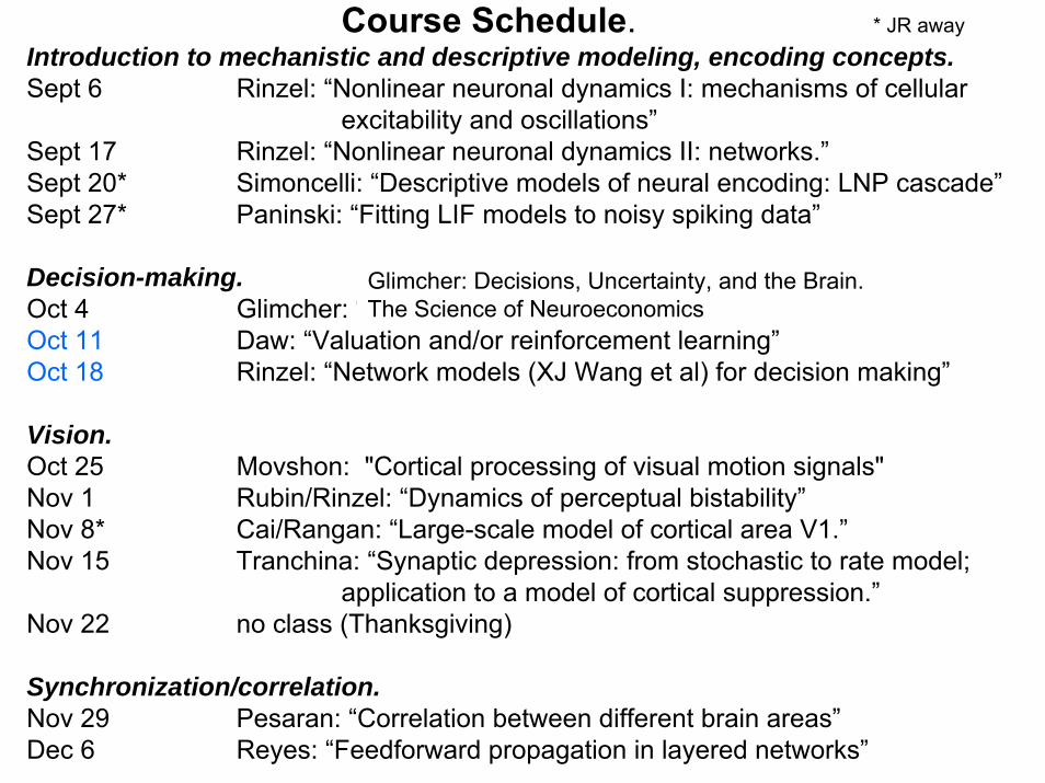
Dynamics of Excitability and Oscillations

Cellular level(spiking)

Network level (firing rate)

Hodgkin-Huxley model Wilson-Cowan model

Membrane currents Activity functions

Activity dynamics in the phase plane

Response modes: Onset of repetitive activity(bifurcations)

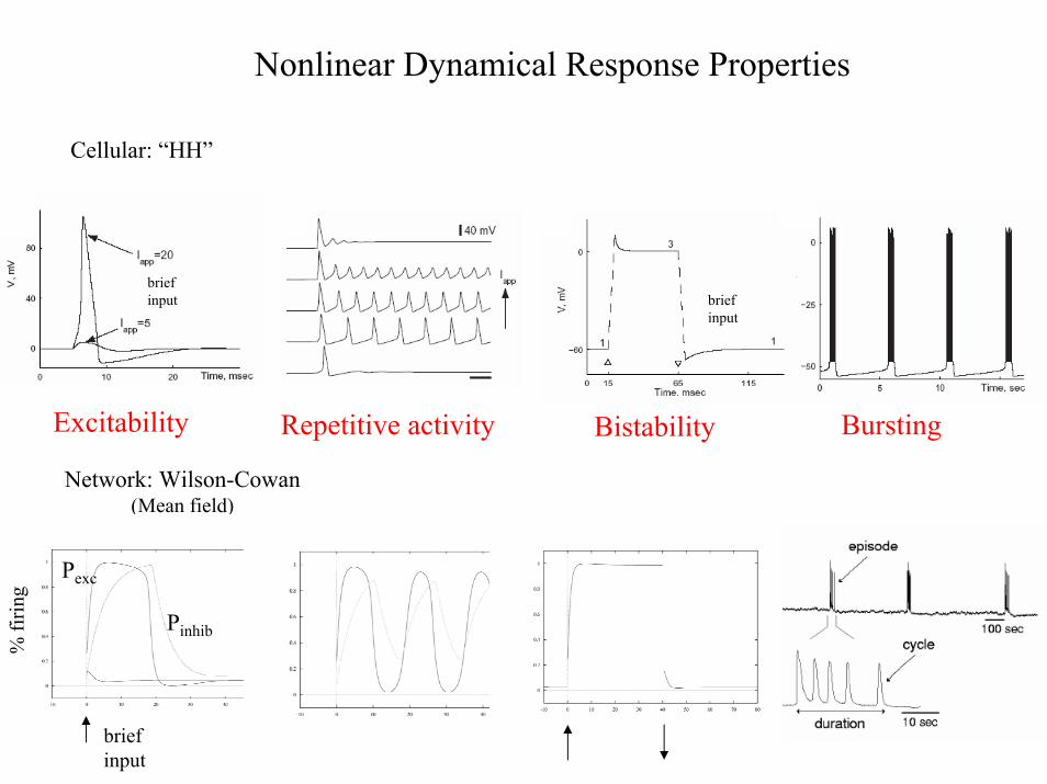
Nonlinear Dynamical Response Properties

Cellular: “HH”

briefinput brief

input

Excitability Repetitive activity Bistability Bursting

Network: Wilson-Cowan(Mean field)

% fi

ring

Pexc

Pinhib

briefinput

Auditory brain stem neurons fire phasically, not to slow inputs. Blocking I KLT may convert to tonic.

J Neurosci, 2002

Take Home Messages

Excitability/Oscillations : fast autocatalysis + slowernegative feedback

Value of reduced models

Time scales and dynamics

Phase space geometry

Different dynamic states – “Bifurcations”; concepts andmethods are general.

XPP software:http://www.pitt.edu/~phase/ (Bard Ermentrout’s home page)

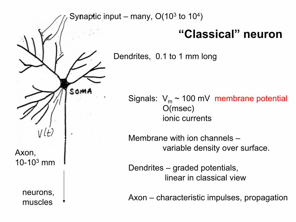
Synaptic input – many, O(103 to 104)

Dendrites, 0.1 to 1 mm long

Axon,10-103 mm

“Classical” neuron

Signals: Vm ~ 100 mV membrane potentialO(msec)ionic currents

Membrane with ion channels –variable density over surface.

Dendrites – graded potentials, linear in classical view

Axon – characteristic impulses, propagationneurons,muscles

Electrical Activity of Cells• V = V(x,t) , distribution within cell

• uniform or not?, propagation?•Coupling to other cells•Nonlinearities•Time scales

∂V ∂ t

∂2 V ∂ x2Cm +Iion(V)= + Iapp + coupling

Current balance equation for membrane:

capacitive channels cable properties other cells

d4Ri

∑ gc,j(Vj–V)

∑ gsyn,j(Vj(t)) (Vsyn-V)

Coupling: “electrical” - gap junctions

j

j

chemical synapsesother cells

= ∑ gk(V,W) (V–Vk )Iion = Iion(V,W)

kchannel types

∂W/∂ t = G(V,W) gating dynamics

generally nonlinear

Nobel Prize, 1959

Current Balance: (no coupling, no cable properties, “steady state” )

0≈ gK(V-VK) + gNa (V-VNa) + gL(V-VL)

V≈LNaK

LLNaNaKK

gggVgVgVg

++++

Replace E by V

HH Recipe:

V-clamp Iion components

Predict I-clamp behavior?

IK(t) is monotonic; activation gate, nINa(t) is transient; activation, m and

inactivation, h

e.g., gK(t) = IK(t) /(V-VK) = GK n4(t)with V=Vclamp

gating kinetics: dn/dt = α(V) (1-n) – β(V) n

= (n∞(V) – n)/τn(V)n∞(V) increases with V.

OFF ONP P*

α(V)

β(V)

mass action for “subunits” or HH-”particles”

INa(t) = GNam3(t) h(t) (V-VNa)

HH Equations

Cm dV/dt + GNa m3 h (V-VNa) + GK n4 (V-VK) +GL (V-VL) = Iapp [+d/(4R) ∂2V/∂x2]

dm/dt = [m∞(V)-m]/τm(V)dh/dt = [h∞(V) - h]/τh(V)dn/dt = [n∞(V) – n]/τn(V)

space-clampedφφφ

φ, temperaturecorrection factor= Q10**[(temp-tempref)/10]

HH: Q10=3

V

Reconstruct action potential

Time courseVelocityThresholdRefractory periodIon fluxesRepetitive firing?

1 µm2 has about100 Na+ and K+

channels.

HH model is a mean-field model that assumes an adequate density of channels.

Bullfrog sympathetic Ganglion “B” cell

Cell is “compact”, electrically … but notfor diffusion Ca 2+

MODEL:

“HH” circuit+ [Ca2+] int+ [K+] ext

gc & gAHP depend on [Ca2+] int

Yamada, Koch, Adams ‘89

Cortical Pyramidal Neuron

Complex dendritic branching Nonuniformly distributed channels

Pyramidal Neuron with axonal tree

Schwark & Jones, ‘89

Koch, Douglas,Wehmeier ‘90

HH action potential – biophysical time scales.

I-V relations: ISS(V) Iinst(V) steady state “instantaneous”

HH: ISS(V) = GNa m∞3(V) h∞(V) (V-VNa) + GK n∞4(V) (V-VK) +GL (V-VL)

Iinst(V) = GNa m∞3(V) h (V-VNa) + GK n (V-VK) +GL (V-VL)

fast slow, fixed at holding valuese.g., rest

Dissection of HH Action Potential

Fast/Slow Analysis - based on time scale differences

h, n are slow relativeto V,m

Idealize AP to 4 phasesV

th,n – constant during

upstroke and downstroke

V,m – “slaved” during plateauand recovery

h,n – constant during upstroke and downstroke

Upstroke…

R and E – stable

T - unstable

C dV/dt = - Iinst(V, m∞(V), hR, nR) + Iapp

R T E

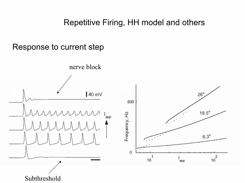
Repetitive Firing, HH model and others

Response to current step

nerve block

Subthreshold

Repetitive firing in HH and squid axon-- bistability near onset

Linear stability: eigenvalues of4x4 matrix. For reduced model w/ m=m∞(V): stability if∂Iinst/∂V + Cm/τn > 0.

Rinzel & Miller, ‘80

HH eqns Squid axon

Guttman, Lewis & Rinzel, ‘80

Interval of bistability

Bistability in motoneurons

2-compartment model; plateau generator in dendrite

Morris-Lecarmembrane model

Booth & Rinzel, ’95

Bistability in 2-compt model

Response to up/down ramp; hysteresis

Switching between states

Two-variable Model Phase Plane Analysis

ICa – fast, non-inactivatingIK -- “delayed” rectifier, like HH’s IK

Morris & Lecar, ’81 – barnacle musclel

VVK VL VCaVrest

negative feedback: slow

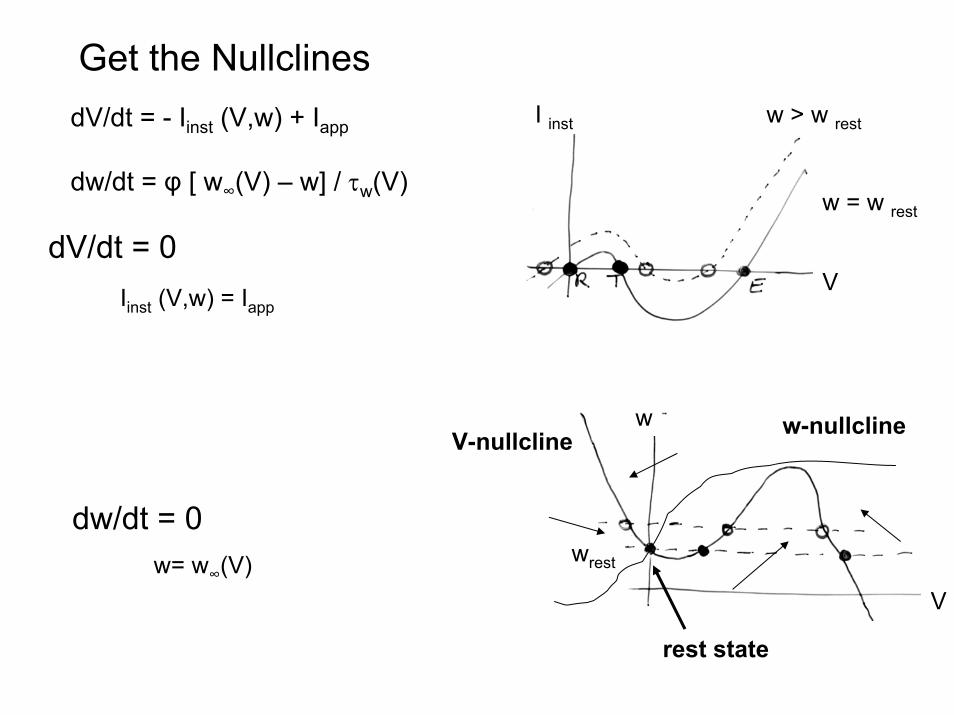
Get the NullclinesdV/dt = - Iinst (V,w) + Iapp

dw/dt = φ [ w∞(V) – w] / τw(V)

V

I inst

w = w rest

w > w rest

dV/dt = 0Iinst (V,w) = Iapp

w

wrest

V-nullcline

V

w-nullcline

rest state

w= w∞(V)

dw/dt = 0

Case of small φ

traj hugs V-nullcline -except for up/downjumps.

ML model- excitableregime

Onset is via Hopf bifurcation

Repetitive Activity in ML (& HH)

“Type II” onsetHodgkin ‘48

Anode Break Excitation or Post-Inhibtory Rebound (PIR)

IK - deactivated

Subthreshold nonlinearities:ipsp can enhance epsp, and lead to spiking

Post inhibitory facilitation, PIF,transient form of PIR

Model of “coincidence-detecting”cell in auditory brain stem. Has a subthreshold K+ current I KLT .

Theory PIF Experiment (Gerbil MSO, slice)

Competing factors:hyperpolar’zn (farther from Vth)and hyperexcitable (reduced w)

Dependence on τinh

Boosting Spontaneous Rate with Fast Inhibition, via PIF

Firing Response to Poisson-Gex train Enhanced by Inhibition (Poisson-Ginh)Gex only: Add Ginh: # of spikes: 10, 15

Std HH model; 100 Hz inputs; τex= τinh=1 ms

w/ R Dodla. PhysRev E, in press

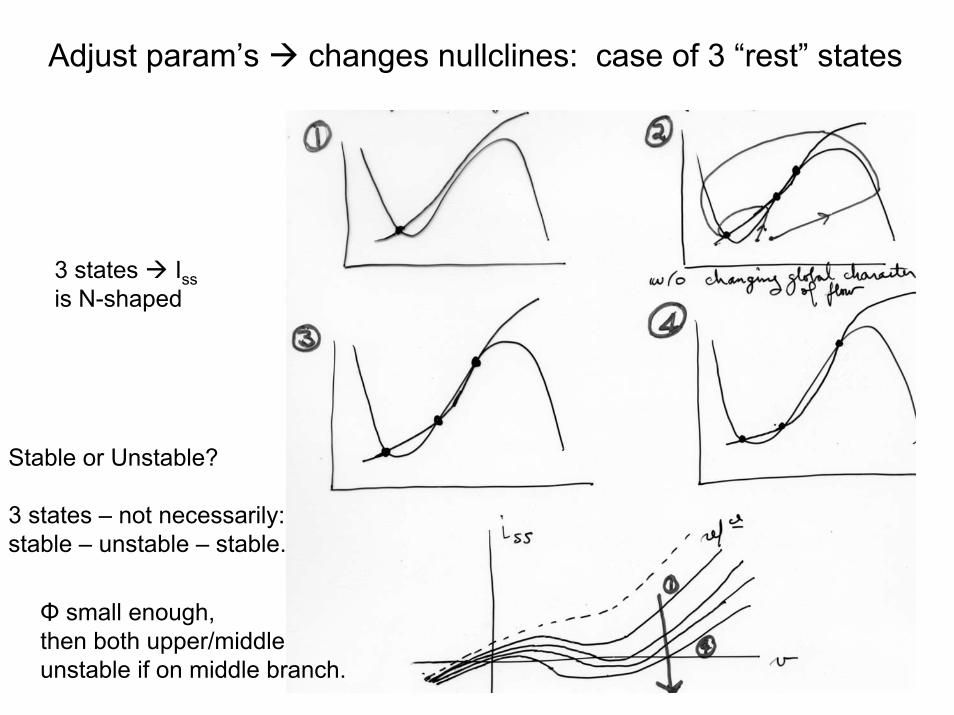
Adjust param’s changes nullclines: case of 3 “rest” states

Stable or Unstable?

3 states – not necessarily:stable – unstable – stable.

3 states Issis N-shaped

Φ small enough,then both upper/middle unstable if on middle branch.

ML: φ large 2 stable steady states

Neuron is bistable: plateau behavior.

Saddle point, with stable and unstable manifolds

V

t e.g., HH with VK = 24 mV

Iapp switching pulses

ML: φ small both upper states are unstable

Neuron is excitable with strict threshold.

thresholdseparatrix long

Latency

Vrest

saddle

IK-A can give long latency but not necessary.

Iss must be N-shaped.

Onset of Repetitive Firing – 3 rest states

SNIC- saddle-node on invariant circle

V

wIapp

excitable

saddle-node

limit cycle

homoclinic orbit;infinite period

emerge w/ large amplitude – zero frequency

Response/Bifurcation diagramML: φ small

freq ~√ I–I1

Firing frequency starts at 0. low freq but no conductancesvery slow

IK-A ? (Connor et al ’77)

“Type I” onsetHodgkin ‘48

Firing rate model (Amari-Wilson-Cowan) for dynamics of excitatory-inhibitory populations.

τe dre/dt = -re + Se(aee re - aei ri + Ie)

τi dri/dt = -ri + Si(aie re – aii ri + Ii)

ri(t), re(t) -- average firing rate (across population and “over spikes”)

τe , τi -- “recruitment” time scale

Se(input) , Si(input) – input/output relations, sigmoids

aee etc – “synaptic weights”

Wilson-Cowan Modeldynamics in the phase plane.

Je

Phase plane, nullclines for range of Je.

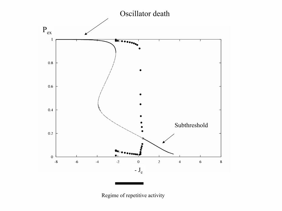
- Je

Pex

Oscillator death

Regime of repetitive activity

Subthreshold

Frequency

- Je

Type I

Type II

“Oscillator Death” but cells are firing

Transition from Excitable to Oscillatory

Type II, min freq ≠ 0Iss monotonicsubthreshold oscill’nsexcitable w/o distinct thresholdexcitable w/ finite latency

Same for W-C network models.

Type I, min freq = 0ISS N-shaped – 3 steady statesw/o subthreshold oscillationsexcitable w/ “all or none” (saddle) thresholdexcitable w/ infinite latency

Hodgkin ’48 – 2 classes of repetiitive firing; Also - Class I less regular ISI near threshold

Noise smooths the f-I relation

Type II

Type I

I app

frequency

FS cellnear threshold

RS cell, w/ noise FS cell, w/ noise

Take Home Message

Excitability/Oscillations : fast autocatalysis + slowernegative feedback

Value of reduced models

Time scales and dynamics

Phase space geometry

Different dynamic states – “Bifurcations”

XPP software:http://www.pitt.edu/~phase/ (Bard Ermentrout’s home page)