Embed Size (px)
Citation preview

1
Computational Methods for the Alignmentand Score-Informed Transcription of Piano
Music
By
Siying WANG
Submitted in partial fulfilment of the requirementsof the Degree of Doctor of Philosophy
London, UK
November 6, 2017
AUTHOR’S DECLARATION
I, Siying Wang, confirm that the research included within this thesis is my ownwork or that where it has been carried out in collaboration with, or supportedby others, that this is duly acknowledged below and my contribution indi-cated. Previously published material is also acknowledged below.
I attest that I have exercised reasonable care to ensure that the work is orig-inal, and does not to the best of my knowledge break any UK law, infringeany third party’s copyright or other Intellectual Property Right, or contain anyconfidential material.
I accept that the College has the right to use plagiarism detection software tocheck the electronic version of the thesis.
I confirm that this thesis has not been previously submitted for the award of adegree by this or any other university.
The copyright of this thesis rests with the author and no quotation from itor information derived from it may be published without the prior writtenconsent of the author.
SIGNATURE: .......................................... DATE: ..........................................
Details of collaboration and publications: See Section 1.3.
2

ABSTRACT
This thesis is concerned with computational methods for alignment and score-informed
transcription of piano music. Firstly, several methods are proposed to improve the align-
ment robustness and accuracy when various versions of one piece of music show complex
differences with respect to acoustic conditions or musical interpretation. Secondly, score
to performance alignment is applied to enable score-informed transcription.
Although music alignment methods have considerably improved in accuracy in re-
cent years, the task remains challenging. The research in this thesis aims to improve the
robustness for some cases where there are substantial differences between versions and
state-of-the-art methods may fail in identifying a correct alignment. This thesis first ex-
ploits the availability of multiple versions of the piece to be aligned. By processing these
jointly, the alignment process can be stabilised by exploiting additional examples of how
a section might be interpreted or which acoustic conditions may arise. Two methods are
proposed, progressive alignment and profile HMM, both adapted from the multiple bi-
ological sequence alignment task. Experiments demonstrate that these methods can in-
deed improve the alignment accuracy and robustness over comparable pairwise methods.
Secondly, this thesis presents a score to performance alignment method that can improve
the robustness in cases where some musical voices, such as the melody, are played asyn-
chronously to others – a stylistic device used in musical expression. The asynchronies be-
tween the melody and the accompaniment are handled by treating the voices as separate
timelines in a multi-dimensional variant of dynamic time warping (DTW). The method
measurably improves the alignment accuracy for pieces with asynchronous voices and
preserves the accuracy otherwise.
Once an accurate alignment between a score and an audio recording is available, the
score information can be exploited as prior knowledge in automatic music transcription
(AMT), for scenarios where score is available, such as music tutoring. Score-informed dic-
tionary learning is used to learn the spectral pattern of each pitch that describes the energy
distribution of the associated notes in the recording. More precisely, the dictionary learn-
ing process in non-negative matrix factorization (NMF) is constrained using the aligned
score. This way, by adapting the dictionary to a given recording, the proposed method
improves the accuracy over the state-of-the-art.
3

ACKNOWLEDGEMENTS
First and foremost, I would like to thank my two wonderful PhD supervisors - SebastianEwert and Simon Dixon. I have been feeling extremely lucky since the first day they agreedto supervise me. Back then, I was confused with my research topic and had strong self-doubt. I simply would not be able to accomplish the work in this thesis without theirinvaluable guidance and encouragement, support and faith in me. They shaped my un-derstanding of good research and showed me the spirit of scientists. I especially want tothank Sebastian for always making the time to discuss with me, despite being very busyhimself.
I want to express my gratitude to Professor Elaine Chew, for being my female rolemodel. I was inspired by Elaine’s attitude toward research and life in general and her ef-forts in gender equality.
The four years I spent in Queen Mary have always been enjoyable, thanks to my dearfriends here. Especially Yading, Chunyang, Chris and Shan. I will never forget the laughand tears we share together, the days and evenings we spent together working and chat-ting. I really appreciate that you are always there whenever I need, offering help and sug-gestions or simply listening. I would also like to thank Maria, Veronica, Mi, Tian, Beici,Simin, Katerina, Sid, Peter, Di, Mattias, Janis, Luwei, Matt, Eita for being great lab-matesand friends.
Thanks for Stella Sick and Werner Goebl for kindly providing the dataset.Last but not least, my deepest thanks go to my family for their unwavering support
and trust. Thanks to my parents for understanding and supporting me in pursuing mydream far from home. Thanks to Fran for your enduring trust, encouragement and caringfor me, for keeping me physically and mentally healthy, sometimes simply by draggingme out from work to a walk, also for proofreading my thesis, discussing with me about myresearch from time to time and always providing good advices.
This work was funded by the China Scholarship Council.
4

TABLE OF CONTENTS
Author’s Declaration 2
Abstract 3
Acknowledgements 4
Table of Contents 8
List of Tables 9
List of Figures 10
List of Symbols 13
1 Introduction 15
1.1 Motivation and Goals . . . . . . . . . . . . . . . . . . . . . . . . . . . . . . . . 15
1.2 Thesis Structure . . . . . . . . . . . . . . . . . . . . . . . . . . . . . . . . . . . 17
1.3 Associated Publications . . . . . . . . . . . . . . . . . . . . . . . . . . . . . . . 19
2 Background 22
2.1 Music Terminology . . . . . . . . . . . . . . . . . . . . . . . . . . . . . . . . . 22
2.1.1 Musical Score . . . . . . . . . . . . . . . . . . . . . . . . . . . . . . . . 23
2.1.2 Musical Performances and Expression . . . . . . . . . . . . . . . . . 24
2.1.3 MIDI Notation . . . . . . . . . . . . . . . . . . . . . . . . . . . . . . . 25
2.2 Feature Representation in Music Alignment . . . . . . . . . . . . . . . . . . . 25
2.2.1 Chroma-based Feature . . . . . . . . . . . . . . . . . . . . . . . . . . 27
5

TABLE OF CONTENTS 6
2.2.2 Decaying Locally adaptive Normalised Chroma Onset (DLNCO)
Features . . . . . . . . . . . . . . . . . . . . . . . . . . . . . . . . . . . 28
2.3 Alignment Methods . . . . . . . . . . . . . . . . . . . . . . . . . . . . . . . . . 29
2.3.1 Dynamic Programming . . . . . . . . . . . . . . . . . . . . . . . . . . 29
2.3.2 Probabilistic Modelling . . . . . . . . . . . . . . . . . . . . . . . . . . 37
2.3.3 Similarity between Dynamic Time Warping and Hidden Markov
Model . . . . . . . . . . . . . . . . . . . . . . . . . . . . . . . . . . . . 43
2.3.4 Other Techniques used in Music Alignment . . . . . . . . . . . . . . 44
2.4 Exploiting Score Information using Alignment Techniques in MIR . . . . . 44
2.4.1 Score-informed Expressive Parameter Extraction . . . . . . . . . . . 44
2.4.2 Score-informed Source Separation . . . . . . . . . . . . . . . . . . . 45
2.4.3 Score-informed Transcription . . . . . . . . . . . . . . . . . . . . . . 46
2.5 Discussion . . . . . . . . . . . . . . . . . . . . . . . . . . . . . . . . . . . . . . 48
3 Robust joint alignment of multiple performances 50
3.1 Introduction . . . . . . . . . . . . . . . . . . . . . . . . . . . . . . . . . . . . . 50
3.2 Motivation . . . . . . . . . . . . . . . . . . . . . . . . . . . . . . . . . . . . . . 51
3.3 Background on Multiple Sequence Alignment . . . . . . . . . . . . . . . . . 52
3.4 Methods for Joint Music Alignment . . . . . . . . . . . . . . . . . . . . . . . . 55
3.4.1 Progressive Alignment . . . . . . . . . . . . . . . . . . . . . . . . . . . 55
3.4.2 Probabilistic Profile . . . . . . . . . . . . . . . . . . . . . . . . . . . . 59
3.4.3 Accelerating Alignments Using Multi-Scale Dynamic Programming 66
3.5 Comparing Pairwise, Progressive and Profile-HMM Based Alignment . . . 67
3.5.1 Dataset and Settings . . . . . . . . . . . . . . . . . . . . . . . . . . . . 69
3.5.2 Comparison Between the Pairwise and Joint Alignments . . . . . . 70
3.5.3 Comparison of the Two Joint Alignment Methods . . . . . . . . . . . 73
3.6 Further Investigations of the Joint Alignment Method . . . . . . . . . . . . . 74
3.6.1 Subset Experiments . . . . . . . . . . . . . . . . . . . . . . . . . . . . 74
3.6.2 Gap Penalty . . . . . . . . . . . . . . . . . . . . . . . . . . . . . . . . . 76
3.6.3 Alignment Order . . . . . . . . . . . . . . . . . . . . . . . . . . . . . . 77
3.6.4 Viterbi Training . . . . . . . . . . . . . . . . . . . . . . . . . . . . . . . 79
3.6.5 Iterative Alignment . . . . . . . . . . . . . . . . . . . . . . . . . . . . . 80

TABLE OF CONTENTS 7
3.6.6 Further evaluation . . . . . . . . . . . . . . . . . . . . . . . . . . . . . 81
3.7 Conclusion . . . . . . . . . . . . . . . . . . . . . . . . . . . . . . . . . . . . . . 82
4 Compensating For Asynchronies Between Musical Voices In Score-
Performance Alignment 84
4.1 Introduction . . . . . . . . . . . . . . . . . . . . . . . . . . . . . . . . . . . . . 84
4.2 Motivation . . . . . . . . . . . . . . . . . . . . . . . . . . . . . . . . . . . . . . 85
4.3 Alignment Method . . . . . . . . . . . . . . . . . . . . . . . . . . . . . . . . . 87
4.3.1 Computing Features for Individual Voices . . . . . . . . . . . . . . . 88
4.3.2 Three-Dimensional Dynamic Time Warping . . . . . . . . . . . . . . 88
4.3.3 Path Constraints . . . . . . . . . . . . . . . . . . . . . . . . . . . . . . 90
4.4 Experiments . . . . . . . . . . . . . . . . . . . . . . . . . . . . . . . . . . . . . 93
4.4.1 Data Set . . . . . . . . . . . . . . . . . . . . . . . . . . . . . . . . . . . 93
4.4.2 Ground Truth Generation . . . . . . . . . . . . . . . . . . . . . . . . . 94
4.4.3 Evaluation Measure . . . . . . . . . . . . . . . . . . . . . . . . . . . . 95
4.4.4 Results . . . . . . . . . . . . . . . . . . . . . . . . . . . . . . . . . . . . 95
4.5 Conclusion and Future Work . . . . . . . . . . . . . . . . . . . . . . . . . . . . 98
5 Identifying Missing and Extra Notes in Piano Recordings Using Score-
Informed Dictionary Learning 100
5.1 Introduction . . . . . . . . . . . . . . . . . . . . . . . . . . . . . . . . . . . . . 100
5.2 Motivation . . . . . . . . . . . . . . . . . . . . . . . . . . . . . . . . . . . . . . 101
5.3 Baseline Method . . . . . . . . . . . . . . . . . . . . . . . . . . . . . . . . . . . 105
5.4 Analysis and Extensions . . . . . . . . . . . . . . . . . . . . . . . . . . . . . . 111
5.4.1 Example of Failure Using the Baseline Method . . . . . . . . . . . . 111
5.4.2 From Spectral Templates to Time-Frequency Patterns . . . . . . . . 113
5.4.3 From Hard to Soft Constraint Regions . . . . . . . . . . . . . . . . . . 114
5.4.4 Encouraging Temporal Continuity in A . . . . . . . . . . . . . . . . . 115
5.4.5 Encouraging Energy Decay in the Template Matrix . . . . . . . . . . 116
5.4.6 Parameter Estimation . . . . . . . . . . . . . . . . . . . . . . . . . . . 116
5.5 Experiments . . . . . . . . . . . . . . . . . . . . . . . . . . . . . . . . . . . . . 118
5.5.1 Dataset & Evaluation Measure . . . . . . . . . . . . . . . . . . . . . . 118

TABLE OF CONTENTS 8
5.5.2 Influence of Individual Parameters . . . . . . . . . . . . . . . . . . . 120
5.5.3 Comparison Between the Baseline Method and Extended Method . 124
5.6 Conclusion . . . . . . . . . . . . . . . . . . . . . . . . . . . . . . . . . . . . . . 125
6 Conclusion 127
6.1 Summary of Contributions . . . . . . . . . . . . . . . . . . . . . . . . . . . . . 127
6.2 Future Directions . . . . . . . . . . . . . . . . . . . . . . . . . . . . . . . . . . 129
6.3 Closing Remarks . . . . . . . . . . . . . . . . . . . . . . . . . . . . . . . . . . . 131
References 133

LIST OF TABLES
2.1 An example of LCS alignment . . . . . . . . . . . . . . . . . . . . . . . . . . . . . 33
3.1 Chopin Mazurkas and their identifiers used in the experiments . . . . . . . . . 69
3.2 Alignment error(mean and standard deviation of average beat deviation in mil-
liseconds) for four types of alignment methods and a random baseline. . . . . 71
3.3 Comparing the Pairwise II alignment method (Ewert et al., 2009b)), Profile
HMM and Progressive Alignment methods in terms of average note onset de-
viation (in milliseconds) . . . . . . . . . . . . . . . . . . . . . . . . . . . . . . . . 81
4.1 Experimental results for three excerpts played with strong asynchrony (upper)
and three pieces without asynchrony (lower). This table shows the number of
performances available and statistics of the alignment error in milliseconds for
the respective pieces. Both results for the 2D-DTW (Ewert et al., 2009b) and our
3D-DTW alignment method are computed separately for the melody (Mel) and
accompaniment (Acc). The error values of these two voices are averaged over
the number of notes to get the overall (OA) alignment error. The change in
alignment error achieved by 3D-DTW is shown in parentheses. . . . . . . . . . 96
5.1 Pieces for evaluation . . . . . . . . . . . . . . . . . . . . . . . . . . . . . . . . . . . 119
5.2 Average Evaluation Results of three Methods for Correctly Played Notes(C), Ex-
tra Notes (E) and Missing Notes (M) . . . . . . . . . . . . . . . . . . . . . . . . . . 125
9

LIST OF FIGURES
2.1 An example of a musical score . . . . . . . . . . . . . . . . . . . . . . . . . . . . . 23
2.2 General framework of music alignment . . . . . . . . . . . . . . . . . . . . . . . 26
2.3 Solving the Dynamic Programming problem with a look-up table . . . . . . . . 31
2.4 An example of DTW alignment for two performance excerpts of Chopin Op. 24
No.2 . . . . . . . . . . . . . . . . . . . . . . . . . . . . . . . . . . . . . . . . . . . . 35
2.5 Multiscale DTW . . . . . . . . . . . . . . . . . . . . . . . . . . . . . . . . . . . . . 36
2.6 An example of HMM model . . . . . . . . . . . . . . . . . . . . . . . . . . . . . . 39
2.7 Non-Negative Matrix Factorisation (NMF) . . . . . . . . . . . . . . . . . . . . . . 45
3.1 A real-world example of pairwise method failing to computer a correct alignment 51
3.2 An example of progressive alignment . . . . . . . . . . . . . . . . . . . . . . . . . 57
3.3 An example of replacing copies of elements with gap symbols after aligning a
new sequence X to the template F , where C (3,2) <C (2,2) and C (5,5) <C (5,4). 59
3.4 Topology of a Profile HMM (Durbin et al., 1999), showing rows of delete states (top),
insert states (middle) and match states (bottom) . . . . . . . . . . . . . . . . . . . . . 60
3.5 An example of Profile HMM . . . . . . . . . . . . . . . . . . . . . . . . . . . . . . 65
3.6 Comparison of the Pairwise II alignment method(Ewert et al., 2009b) with the
proposed progressive alignment method and profile HMM method . . . . . . . 71
3.7 Histograms of beat deviation using the Pairwise II alignment method (Ewert
et al., 2009b), the progressive alignment and profile HMM method. . . . . . . . 73
3.8 Comparison between the Pairwise II alignment method (Ewert et al., 2009b)
and two joint alignment methods for subset experiments. . . . . . . . . . . . . 75
10

LIST OF FIGURES 11
3.9 Average beat deviation (ABD) values for the five Mazurka pieces with progres-
sive alignment using a gap-less variant and different values of gap penalty,
compared with the Pairwise II alignment method(Ewert et al., 2009b). The
cross markers represent the mean ABD and the error bars show the standard
deviation. . . . . . . . . . . . . . . . . . . . . . . . . . . . . . . . . . . . . . . . . . 76
3.10 Average beat deviation (ABD) values for the five Mazurka pieces with progres-
sive alignment using different alignment orders and the iterative extension,
compared with the Pairwise II alignment method (Ewert et al., 2009b). . . . . 77
3.11 The convergence of average beat deviation with increasing number of itera-
tions for two model learning methods for the profile HMM. . . . . . . . . . . . 80
4.1 An example of asynchronies between the melody and the accompaniment . . 86
4.2 A three-dimensional cost tensor. . . . . . . . . . . . . . . . . . . . . . . . . . . . 89
4.3 Constraining the 3D-DTW alignment . . . . . . . . . . . . . . . . . . . . . . . . . 92
4.4 A GUI for manually correcting the alignment between the performance MIDI
and score MIDI . . . . . . . . . . . . . . . . . . . . . . . . . . . . . . . . . . . . . . 94
4.5 Comparison of the 2D-DTW with the proposed 3D-DTW alignment results. . . 97
4.6 Comparison between the ground truth (red) and detected asynchronies (green)
between the melody and the accompaniment for a performance of Chopin
Op. 3 No. 10 (first 21 measures). . . . . . . . . . . . . . . . . . . . . . . . . . . . . 98
5.1 Score-Informed Transcription . . . . . . . . . . . . . . . . . . . . . . . . . . . . . 102
5.2 Score-Informed Dictionary Learning . . . . . . . . . . . . . . . . . . . . . . . . . 106
5.3 Adaptive and pitch-dependent thresholding . . . . . . . . . . . . . . . . . . . . 109
5.4 A problematic case where the baseline method summarised in Section 5.3
failed while the proposed extensions work correctly . . . . . . . . . . . . . . . . 112
5.5 Plot of function f (x) = (γx −1)e(γx−1) for γ= 10. . . . . . . . . . . . . . . . . . . 117
5.6 Average accuracy as a function of different parameters. (a) activation con-
straint ζ1; (b) diagonal structure regulariser ζ2; (c) activation sparsity regu-
lariser ζ3; (d) spectral continuity regulariser; (e) template constraint η2; (f) de-
cay regulariser η3 . . . . . . . . . . . . . . . . . . . . . . . . . . . . . . . . . . . . 121

LIST OF FIGURES 12
5.7 Interaction between parameters ζ2 and η2 as they influence identification ac-
curacy for all three types of notes. . . . . . . . . . . . . . . . . . . . . . . . . . . . 124
LIST OF SYMBOLS
α The forward matrix in the Baum Welch Training procedure;
β The backward matrix in the Baum Welch Training procedure;
η The weight of regulariser term on the spectral template matrix;
F A feature space;
γ Its entry γn(i ) is defined as the probability of being in the state si at
the frame n given the model λ and the observation sequence O
λ A Hidden Markov Model (HMM);
A The index set of the attack templates for a pitch;
B The index set of the sustain templates for a pitch;
µ The mean vector of the Gaussian observation distribution in an
HMM;
Φ The size of constraint region in 3D-DTW;
π= (π0,π1, . . . ,πL) The initial state distribution in an HMM;
ψ A lookup table/matrix to store the best choice of each step in Dy-
namic Programming;
σ The covariance matrix of the Gaussian observation distribution in
an HMM;
Θ The maximally allowed asynchrony in 3D-DTW;
13

LIST OF SYMBOLS 14
ξ Its entry ξn(i , j ) is defined as the probability of being in the state si
at frame n and transiting to s j at time n +1, given the model λ and
the observation sequence O;
ζ The weight of regulariser term on the activation matrix;
A The activation matrix;
ai j The state transition probability;
bi (On) The observation probability;
C A dissimilarity/similarity matrix;
c A local dissimilarity/similarity measure on F ;
D A total dissimilarity/similarity matrix;
F The template data structure in a progressive alignment;
G The gap symbol in a progressive alignment;
K The number of versions of a piece used in a multiple alignment;
L The number of states in an HMM;
N The length of the observation sequence in an HMM;
O = (O1,O2, . . . ,ON ) An observation sequence in an HMM;
P The spectral template matrix;
p An alignment;
S = (s1, s2, . . . , sL) States in an HMM;
V The magnitude spectrogram;
w The weight to adjust the preference over the three step sizes in the
alignment;
X ,Y ,Z Feature sequences with their elements xn ∈F , ym ∈F and zl ∈F ;

CH
AP
TE
R
1INTRODUCTION
1.1 Motivation and Goals
The last few decades have seen a revolution in the way people interact with music, includ-
ing how we make, store, share, learn and enjoy music. These developments have led to
the explosive growth of digital music collections and music-related data. Music content
providers (e.g. Spotify, iTunes, Pandora) rely on their existence, while national libraries
and charitable organisations create and curate them in order to provide access to cul-
tural heritage. For one piece of music, large collections often contain various recordings,
videos, annotations and other metadata. In particular for Western classical music, there
are often multiple versions associated with any given piece of music, including different
editions of the sheet music, various types of symbolic representations (such as MIDI - Mu-
sical Instrument Digital Interface and MusicXML - Music Extensible Markup Language)
and multiple recordings of musical performances (in the form of audio recordings or MIDI
files).
To establish links between different versions of a piece of music, various music align-
ment methods have been proposed in recent years. The goal of music alignment is to
map each temporal position in one version of a piece of music to the corresponding po-
sition in another version of the same piece. During the last decades, such methods have
15

CHAPTER 1. INTRODUCTION 16
been of central importance for analysing, modelling and processing music signals. They
have enabled a multitude of applications, including automatic score following and page
turning (Arzt et al., 2014; Montecchio and Cont, 2011a), facilitated navigation in large col-
lections (Müller et al., 2010), the identification of cover songs (Serrà et al., 2008), query-
by-example retrieval (Casey et al., 2008) and the integration of prior knowledge in audio
source separation (Ewert et al., 2014).
Various alignment methods have been proposed, including Dynamic Time Warping
(DTW) (Hu et al., 2003), Hidden Markov and Semi-Markov Models (HMM) (Orio and
Déchelle, 2001), Conditional Random Fields (CRF) (Joder et al., 2011), general graphical
models (Raphael, 2004), and Particle Filter / Monte-Carlo Sampling (MCS) based meth-
ods (Montecchio and Cont, 2011a; Duan and Pardo, 2011). The performance of alignment
methods has improved considerably over the years. As shown in previous studies, cur-
rent methods yield a high accuracy in many cases (Joder et al., 2011; Ewert et al., 2009b;
Dixon and Widmer, 2005). However, the task remains challenging. For cases with strong
local differences between versions, even state-of-the-art methods may fail to identify the
correct alignment. Such strong local differences often stem from two aspects. On the one
hand, the acoustic conditions may vary regarding recording environment and instrumen-
tation. On the other hand, musicians can interpret a piece in diverse ways with respect
to the articulation, expressive timing, embellishments or the relative loudness of notes
(balance).
The first goal of this thesis is to improve the alignment robustness against such strong
local differences by developing novel alignment methods. Under this goal, the first idea is
to make use of the information provided by multiple versions of a piece of music to sta-
bilise the alignment process. Most state-of-art methods align two versions in a pairwise
fashion, which may not be robust enough against substantial local differences. However,
in many scenarios not only two but multiple versions of a given piece are available, espe-
cially for Western classical music. By processing multiple versions jointly, the alignment
process can be provided with additional examples of how a section might be interpreted or
which acoustic conditions may arise. This can help especially with sections where strong
local differences are shown between any two versions.
The second idea to improve robustness and accuracy stems from a commonly used

CHAPTER 1. INTRODUCTION 17
musical parameter: the asynchrony between voices. Current methods typically assume
that notes occurring simultaneously in the score are played concurrently in a perfor-
mance. However, musicians sometimes introduce asynchronies between simultaneous
notes as a device of music expression. Such asynchronies may locally lead to a measur-
able drop in alignment accuracy because they are not taken into consideration by current
methods. To handle such asynchronies, an idea presented in this thesis is to separate the
melody and accompaniment voices in the score and compute a three-dimensional align-
ment between the two score timelines and the audio timeline. To lower the computational
cost and improve the overall robustness, the standard two-dimensional alignment is used
to constrain the computation in the proposed method.
A more accurate and robust alignment as provided by the two above methods is useful
for various applications. One of them is to exploit the score information to analyse audio
recordings of the same piece. The second goal of this thesis is thus to apply score to au-
dio alignment to build a score-informed music transcription method. Automatic music
transcription aims at obtaining a high-level symbolic representation of the notes played
in a given audio recording. However, the performance of current methods is inadequate
for many applications. The idea presented in this thesis is to provide score information,
available in certain scenarios, as prior knowledge to the transcription system, in order to
boost its accuracy. Such a method is particularly interesting for a specific application: mu-
sic tutoring, in which the system provides feedback on when and how the student deviates
from the given score. The alignment between the audio recording and the corresponding
score indicates for each score note, an approximate time position in the audio. This infor-
mation is used to construct a transcription method that is tailored to the given recording
by a score-informed dictionary learning method.
Overall, this thesis aims to propose computational methods for both alignment and
score-informed transcription. Although the methods are applicable to other genres of
music, this thesis focuses on Western classical piano music.
1.2 Thesis Structure
The contribution of this thesis is two-fold. Firstly, it proposes novel alignment methods for
two different scenarios, in Chapter 3 and Chapter 4 respectively. Secondly, it applies the

CHAPTER 1. INTRODUCTION 18
alignment methods to build a score-informed music transcription system in Chapter 5.
This section describes the structure of this thesis and provides a brief introduction to each
chapter.
Chapter 1 is the introduction to the thesis. It explains its motivation and goals, fol-
lowed by a description of thesis structure. Associated publications are listed at the end
and their contributions to this thesis are specified.
Chapter 2 provides the background knowledge and core concepts which are used
throughout the thesis. Some general related work is also mentioned there, while works
specific to a certain chapter are discussed in the corresponding chapters. The chapter
starts with a summary of different representations of music and related terminology, in-
cluding the music score, the notion of performance and expression as well as MIDI nota-
tion. It then discusses two concepts used in alignment: feature representation and algo-
rithms/methods. As feature design is not the focus of this thesis, it only mentions features
commonly used in music alignment and describes the features used in Chapter 3 and
Chapter 4. A discussion of alignment methods is given afterwards. The main description
focuses on two categories of methods: Dynamic Programming and Probabilistic Mod-
elling, which are both used in later chapters. Last but not least, the chapter provides an
overview of score-informed Music Information Retrieval (MIR) research based on music
alignment techniques, including score-informed source separation and score-informed
music transcription to prepare the reader for Chapter 5.
Chapter 3 aims at increasing alignment robustness against strong local differences
by exploiting the availability of multiple versions of the piece to be aligned. Inspired by
the multiple sequence alignment problem in bio-informatics, this chapter proposes two
joint alignment methods to process multiple performances. The two proposed methods
are conceptually different but share some similarities from an algorithmic point of view.
Experiments show that both of them can improve the alignment accuracy and robust-
ness. Further, this chapter investigates their behaviours and compares them with respect
to their computational efficiency and alignment accuracy.
Chapter 4 focuses on improving the alignment accuracy for cases with strong asyn-
chronies between the melody and the accompaniment voice. It presents a novel score
to performance alignment method that treats the two score voices in separate timelines

CHAPTER 1. INTRODUCTION 19
and computes a joint three dimensional alignment using an extended version of Dynamic
Time Warping (DTW) between them and the audio timeline using information obtained
via classical DTW. Two types of constraints for the calculation of the cost matrix are pro-
posed to lower the computational costs and to improve the overall alignment accuracy.
Experiments show that the proposed method measurably improves the alignment accu-
racy for pieces with asynchronous voices and preserves the accuracy otherwise.
Chapter 5 presents a score-informed transcription system for identifying missing and
extra notes from piano recordings. To improve the accuracy of automatic music transcrip-
tion, the idea of this chapter is to exploit the music score as prior knowledge by applying
score to audio alignment. A score-informed dictionary learning method is used to con-
struct a transcription system that is tailored to the given audio recording. This chapter
also analyses a case where the system fails, and designs several countermeasures to im-
prove the performance. The influence of these extensions are investigated with further
experiments.
Chapter 6 concludes the thesis and discusses possible directions for future work.
1.3 Associated Publications
Most of the work in this thesis has been published in international peer-reviewed confer-
ences and journals, as listed below. How each paper relates to each chapter is specified
accordingly.
1. (Wang et al., 2014) S. Wang, S. Ewert, and S. Dixon. Robust Joint Alignment of Mul-
tiple Versions of A Piece of Music, Proceedings of the International Society for Music
Information Retrieval Conference (ISMIR), Taipei, Taiwan, 2014
This paper proposes a novel method to align multiple versions of a piece of music
in a joint manner, which stabilises the alignment process and leads to an increase
in alignment robustness. It is the basis of (Wang et al., 2016).
2. (Wang et al., 2016) S. Wang, S. Ewert, and S. Dixon. Robust and Efficient Joint Align-
ment of Multiple Musical Performances, IEEE/ACM Transactions on Audio, Speech
and Language Processing, 24(11), 2016
This paper extends (Wang et al., 2014). It presents two joint alignment methods,

CHAPTER 1. INTRODUCTION 20
progressive alignment and probabilistic profile, and discusses their fundamental
differences and similarities on an algorithmic level. It also provides an in-depth
analysis of both joint alignment methods and shows that both methods can im-
prove the alignment robustness as well as the accuracy over comparable pairwise
methods. It is the basis of Chapter 3.
3. (Wang et al., 2015) S. Wang, S. Ewert, and S. Dixon. Compensating For Asynchronies
Between Musical Voices In Score-Performance Alignment, Proceedings of the IEEE
International Conference on Acoustics, Speech, and Signal Processing (ICASSP),
Brisbane, Australia, 2015 (Best Student Paper Award for the Audio and Acoustic Sig-
nal Processing track)
This paper presents a score to audio alignment method that can handle asyn-
chronies between the melody and accompaniment by treating the voices as sepa-
rate timelines in a multi-dimensional variant of dynamic time warping (DTW). It is
the basis for Chapter 4.
4. (Ewert et al., 2016) S. Ewert, S. Wang, M. Müller and M. Sandler. Score-Informed
Identification of Missing and Extra Notes in Piano Recordings, Proceedings of the In-
ternational Society for Music Information Retrieval Conference (ISMIR), New York,
USA, 2016
This paper proposes a score-informed transcription method for identifying missing
and extra notes in piano recordings. The score information is used to constrain a
dictionary learning process based on non-negative matrix factorisation (NMF), so
that the learned dictionary is highly adapted to the given recording. This paper lays
the ground work for Chapter 5.
5. (Wang et al., 2017) S. Wang, S. Ewert, and S. Dixon. Identifying Missing and Ex-
tra Notes in Piano Recordings Using Score-Informed Dictionary Learning, IEEE/ACM
Transactions on Audio, Speech and Language Processing (Available online publica-
tion), 2017
This paper extends (Ewert et al., 2016). It identifies several systematic weaknesses in
the previous work and introduces three extensions as countermeasures to improve

CHAPTER 1. INTRODUCTION 21
the performance of the proposed system. The influence of each extension is investi-
gated, and experiments show that they indeed improve the accuracy for identifying
extra notes. It is the basis for Chapter 5.
For publications 1-3 and 5, I developed the corresponding methods, conducted all the
experiments and wrote the articles. Sebastian Ewert and Simon Dixon co-supervised my
work, providing ideas and suggestions for the method and experimental design, as well as
comments and corrections for the articles. For publication 4, Sebastian Ewert developed
the method, conducted the experiments and wrote the paper. I helped with the exper-
iments. Meinard Müller and Mark Sandler provided comments and corrections for the
article.

CH
AP
TE
R
2BACKGROUND
This chapter provides the background knowledge for this thesis. First, Section 2.1 will
introduce some music terminology used throughout the thesis in this thesis. Next, Sec-
tion 2.2 will describe audio features used in the music alignment task. A discussion of
music alignment methods will be given in Section 2.3, followed by an overview of score-
informed Music Information Retrieval (MIR) research based on music alignment tech-
niques in Section 2.4.
2.1 Music Terminology
A piece of music, especially Western classical music, is often associated with multiple ver-
sions or representations, including sheet music of different editions, symbolic representa-
tions of various types such as MIDI (Musical Instrument Digital Interface ) and MusicXML
(Music Extensible Markup Language), or audio recordings of different performances. Each
type of representation describes a different perspective on the piece and serves a different
purpose. Composers use the score representation to provide detailed instructions on how
to perform the music piece they created, while there is a certain degree of freedom for
performers to interpret with different musical expression. In the following, the concept
22

CHAPTER 2. BACKGROUND 23
Figure 2.1: An example of music score: Liszt, Franz, Étude en douze exercices, S.136, No.1(C major), bars 1-3
of musical score and performance will be introduced, followed by MIDI, a music notation
format used in this thesis.
2.1.1 Musical Score
A musical score is regarded as the most fixed reference for the Western classical reper-
toire (Howat, 1995). Among various genres, Western classical music (which is the genre
of interest in this thesis) has relatively little freedom in interpreting a piece and demands
for a stricter adherence to the score, compared to genres such as jazz which grant a larger
degree of improvisation (Cook, 2014; Miotto et al., 2010).
However, many details on the score are open to interpretation, especially the expres-
sive markings. Examples include tempo markings such as Vivace (meaning lively and fast)
and Ritardando (meaning gradually slowing down), dynamic markings such as p (mean-
ing soft) and mf (meaning medium loud), articulation markings such as staccato (mean-
ing shorten the note duration and separate from the following note) and fermata (mean-
ing a pause on the current note), ornament markings such as trills and grace notes, pedal
markings, or even descriptive words for expressive musical ideas such as arpeggio (mean-
ing broken chord) and con fuoco (meaning with fire). Figure 2.1 shows the first three bars
of Liszt’s Étude en douze exercices, S.136, No.1 (C major) with various music symbols.
These descriptive notations lead to many possible interpretations, subject to the playing
time, the circumstances, the performer and many other factors. For example, Debussy
explained for his descriptive or implicit pedalling notation (Nichols, 1992; Howat, 1995)
"Pedalling cannot be written down: it varies from one instrument to another,
from one room, or one hall, to another"

CHAPTER 2. BACKGROUND 24
Additionally, the score itself may vary between different editions, due to the composer’s
copying and revising processes, corrections or additions from editors, or printing conven-
tions (Howat, 1995).
2.1.2 Musical Performances and Expression
Many musicologists agree that the score is merely a "ghostly instantiation" of the musi-
cal work (Thomas and Smiraglia, 1998), while a performance of the piece is considered to
be a more complete rendition because it turns the abstract content in the score to a con-
crete realisation in real time. Musical works are collaborations between composers and
performers and they may accrue new meanings decades or even centuries after compo-
sition (Cook, 2014). Performers study the idiom of the composers through the score and
reproduce the music with their very own expression. In this sense, the score is a guidance
which cannot capture all the possible nuances of performances and every performance is
a new creation of the musical work.
Within the constraints set by the structure of a composition, the performer can ma-
nipulate various expressive features to shape the musical work (Clarke, 1995), including
tempo, timing, dynamics, timbre and articulation. For example, melody lead (which will
be discussed in Chapter 4), is an expressive feature in which the performer emphasises
the melody in multi-voice music by playing the melody louder and preceding other voices
by around 30ms (Goebl, 2000).
Since an early investigation led by Seashore (1938), music performance research has
been an active field for several decades (Fabian et al. (2014) have provided a comprehen-
sive overview). Modern computational methods enable the large scale measurement and
analysis of the nuances in musical expression, a process which previously was carried out
manually and thus was limited to small-scale studies (Goebl et al., 2008). One approach to
acquiring expression data is to use specifically equipped instruments, such as the Yamaha
Disklavier system and Bösendorfer’s SE and CEUS systems. They record the performance
not as an audio recording, but in some symbolic formats which describe each note event,
such as MIDI.

CHAPTER 2. BACKGROUND 25
2.1.3 MIDI Notation
The MIDI (Musical Instrument Digital Interface) standard specifies a protocol for commu-
nication between electronic instruments (Chapman and Chapman, 2000). Instead of the
sound waveform, MIDI carries the control data that encodes musical performance infor-
mation (Roads, 1996), such as the start and stop time of a note, its pitch and its velocity1
as well as clock messages for synchronisation purposes. The playback timbre and qual-
ity depends on the device that receives the MIDI message. Roads (1996) has provided a
comprehensive introduction to the MIDI standard.
MIDI is widely used as a symbolic representation of a musical score. It stores the inter-
nal structure of the score in a sequence of MIDI messages. Although it cannot represent
the graphical layout of the score and it is not able to store the expression markings, it is
lightweight and universally compatible, and therefore most online digital score resources
use the MIDI format. MIDI-format scores are used in the experiments in this thesis.
MIDI can also be used to record musical performances. MIDI compatible instruments
such as synthesiser keyboards or digital pianos are used to capture clean expressive data
from music performances in MIDI format, without the noise or reverberation which are
unavoidable in the audio recordings. Furthermore, by offerering playback of MIDI files,
the computer-monitored acoustic pianos such as the Yamaha Disklavier and Bösendor-
fer’s SE and CEUS series combine the sound quality of the acoustic piano and the ability
to record a performance in MIDI format. Such pianos are widely used in music perfor-
mance study(Goebl et al., 2008; Gabrielsson, 2003; Cook, 2014; Goebl, 2000) and even in
piano competitions2. In this thesis, MIDI representations of performances will be used as
ground truth annotations of the pitch and timing of notes, as well as to be synthesised to
audio for part of the evaluation.
2.2 Feature Representation in Music Alignment
As a fundamental problem in MIR, music alignment research has been active for sev-
eral decades. The general principle used by most music alignment methods consists of
1For a MIDI instrument that has velocity sensing, velocity is usually related to the speed with which theinstrument is being hit, thus the higher the velocity the louder the note. For example, for the Disklavier piano,the hammer velocity is recorded.
2www.piano-e-competition.com

CHAPTER 2. BACKGROUND 26
Figure 2.2: General framework of music alignment includes two steps: 1. Extract featuresfrom different versions of a piece of music with a common feature representation; 2. Alignfeature sequences in a suitable alignment method. Alignment can be applied in variousscenarios (such as automatic score following (Arzt et al., 2014) and page turning (Montec-chio and Cont, 2011a))
two main steps, illustrated in Figure 2.2. First, the files to be aligned including various
types of score and audio representations, are converted into feature sequences. Then the
feature sequences are compared to find an optimal mapping using some suitable align-
ment methods. Early approaches before the ’90s (Dannenberg, 1984; Vercoe, 1984) were
designed to align symbolic music representations such as MIDI. In recent years, the in-
crease in computational power has enabled the processing of audio signals, and thus the
last decades have seen efforts shifting towards robust feature representations and suitable
alignment methods for aligning audio recordings.
For the feature representation, a major aim is to find an optimal, application-specific
trade-off between the level of detail preserved in a feature and its robustness against noise
and other musically irrelevant signal properties. In this context, low-level spectral rep-
resentations have been used (Orio and Schwarz, 2001; Turetsky and Ellis, 2003; Cont,
2010) as well as musically motivated representations, especially pitch and chroma fea-
tures (Dannenberg and Hu, 2003; Müller et al., 2005; Cont, 2006). More recently, it was
found that accompanying such representations with features indicating onset positions
can be used to improve the alignment accuracy (Ewert et al., 2009b; Joder et al., 2011).
Other more recent developments are adaptive or employ learnt feature representations

CHAPTER 2. BACKGROUND 27
(Cont, 2006; Niedermayer, 2009a; Joder et al., 2013; Raffel and Ellis, 2015).
In the following, two types of features will be introduce, which will be used throughout
this thesis, chroma-based features and onset indicating features.
2.2.1 Chroma-based Feature
A fundamental phenomenon in music is "octave equivalence", i.e. the observation that
pitches exactly one or more octaves apart are musically equivalent in many ways and are
perceived as similar in "colour" by listeners. In the early 1960s, Shepard (1964) reported
the circularity in pitch perception. He represented the frequency of each pitch with two
dimensions, "height" and "tonality /tone chroma", which are essentially the "octave num-
ber" and "pitch class" in music theory. In a standard Western 12-tone system, each octave
consists of 12 pitches and pitches one or more octaves apart have the same chroma value,
from the set {C ,C #,D,D#,E ,F,F #,G ,G#, A, A#,B} (here C #/D[ etc are treated as equiva-
lent).
Given the cyclic property of pitch perception, it is appropriate to use chroma based
features in music processing. Fujishima (1999) proposed a Pitch Class Profile (PCP) fea-
ture, which maps spectrum bin indices to the corresponding chroma index, and which
the authors used in a chord recognition system. In the same year, Wakefield (1999) pre-
sented a very similar idea, the Chromagram, which maps the frequency dimension of the
spectrogram into 12 pitch classes. Since then, chroma based features have raised a con-
siderable amount of research interest and the following decade saw considerable efforts in
designing such features and improving their robustness. For example, Bartsch and Wake-
field (2001) employed beat-synchronous frame segmentation for the chroma feature, in
order to gain invariance to tempo changes. Gómez (2006) extended PCP to Harmonic
Pitch Class Profiles (HPCP), by weighting the contributions of each harmonic for each
pitch, to minimise the influence of tuning differences and inharmonicity. Müller and
Ewert (2010) proposed CRP (Chroma DCT-Reduced log Pitch) as a feature robust against
timbre variation which was achieved by discarding low-order cepstral coefficients which
contain information closely related to timbre.
Chroma based features have been used in various MIR tasks, as they encode harmonic
relationships (Bartsch and Wakefield, 2005) which are very important in analysing music
CHAPTER 2. BACKGROUND 28
signals. Applications include chord recognition (Peeters, 2006; Bello and Pickens, 2005;
Cho et al., 2010; Fujishima, 1999; Harte and Sandler, 2005; Mauch and Dixon, 2010; Sheh
and Ellis, 2003), music structural analysis (Bartsch and Wakefield, 2001, 2005; Chai, 2006;
Dannenberg and Goto, 2008; Paulus et al., 2010), as well as music matching and align-
ment (Kurth and Müller, 2008; Müller et al., 2005; Hu et al., 2003; Joder et al., 2010; Müller,
2007).
2.2.1.1 Chroma Energy Normalised Statistics (CENS) feature
Chapters 3 and 5 employ the CENS (Chroma Energy Normalised Statistics) feature, pro-
posed by Müller et al. (2005). It is obtained by calculating short-time statistics over the
chroma energy distribution, to increase the robustness against variations in timbre, dy-
namics and articulation. Specifically, the audio is firstly converted to a sequence of
chroma vectors. Each chroma vector is then normalised by the sum of its energy in all
12 chroma bands, in order to absorb variations in dynamics. Next, each chroma vector is
quantised to several levels. After that, the sequence of quantised chroma vectors is con-
volved component-wise by a Hann window and then downsampled. To this end, each
feature represents a weighted statistic of the energy distribution over the window size, to
smooth out the local time deviations.
2.2.2 Decaying Locally adaptive Normalised Chroma Onset (DLNCO) Features
Besides the widely used chroma features, the experiments of this thesis use another type
of feature: DLNCO (Decaying Locally adaptive Normalised Chroma Onset) feature. It was
proposed by Ewert et al. (2009b) and experiments showed that the combination of chroma
and DLNCO features largely improves alignment accuracy for music with clear note at-
tacks such as piano music.
To obtain the DLNCO feature, firstly a local energy curve is computed for each MIDI
pitch and the energy peaks are chosen as onset features. The pitch based onset features
from the same pitch class are summed up into 12-dimensional chroma onset features.
The analogy to chroma features is used to enhance the robustness against timbre variation
while still preserving a notion of which note was played. Next, the features are normalised

CHAPTER 2. BACKGROUND 29
in a locally adaptive fashion to further improve the robustness against local dynamic vari-
ation. At the end, an additional temporal decay structure is employed, so that when DL-
NCO feature sequences are compared using the Euclidean distance, a diagonal corridor of
low cost will appear where the onset vectors are similar, therefore only significant events
take effect on the cost matrix level.
2.3 Alignment Methods
After a suitable feature representation is chosen, different versions of a piece of music are
converted to sequences of this common feature representation. The next step is to align
the resulting feature sequences with a suitable method. Without losing the generality,
the following considers the case of aligning two versions of a piece of music. Let X :=(x1, x2, . . . , xN ) and Y := (y1, y2, . . . , yM ) be two feature sequences with xn , ym ∈F , where F
denotes a suitable feature space. An alignment between X and Y is defined as a sequence
p = (p1, . . . , pL) with p` = (n`,m`) ∈ [1 : N ]×[1 : M ] for ` ∈ [1 : L]. satisfying 1 = n1 ≤ n2 ≤. . . ≤ nL = N and 1 = m1 ≤ m2 ≤ . . . ≤ mL = M (boundary and monotonicity conditions), as
well as p`+1−p` ∈ {(1,0), (0,1), (1,1)} (step size condition). Each step p` matches elements
xn and ym .
Various alignment methods have been proposed, including Dynamic Time Warping
(DTW) (Müller, 2007), Hidden Markov Models (HMM) (Raphael, 1998), Conditional Ran-
dom Fields (CRF) (Joder et al., 2011), general graphical models (Raphael, 2004), and Par-
ticle Filter / Monte-Carlo Sampling (MCS) based methods (Montecchio and Cont, 2011a;
Duan and Pardo, 2011). The choice of methods varies with the application scenarios. For
example, when aligning symbolic music such as MIDI, string matching based methods
are often used (Dannenberg, 1984; Chen et al., 2014). In recent work, a convolutional neu-
ral network has been used in sheet music to audio alignment (Dorfer et al., 2016a). While
numerous methods have been used for the music alignment task, many of them fall into
two wide categories, Dynamic Programming and Probabilistic Modelling.
2.3.1 Dynamic Programming
Dynamic programming is an often used algorithmic approach to certain optimisation
problems. The main idea is to break down a problem to into sub-problems and combine

CHAPTER 2. BACKGROUND 30
their solutions successively to obtain the final solution for the original problem. In the
context where dynamic programming is applied, those sub-problems overlap with each
other in some sense. Instead of recomputing the solution to reoccurring sub-problems,
the algorithm stores the solution to a sub-problem in a look-up table and simply retrieves
the corresponding solution next time the same sub-problem occurs.
We can apply Dynamic Programming methods to the alignment problem by viewing
finding the best match between sequences as an optimisation problem. Its objective is
to obtain an optimal alignment minimising the dissimilarity or maximising the similarity
between features assigned to each other. Without loss of generality, we refer to similarity
in this section. The similarity is calculated by a certain similarity measure, depending on
the specific algorithm. The following paragraphs explain the idea behind using Dynamic
Programming for alignment and some specific algorithms will be described in the next
sections.
To align two feature sequences X and Y , let c : F ×F → R denote a local similarity
measure on F . Define a resulting (N ×M) similarity matrix C by C (n,m) := c(xn , ym). The
total similarity is the sum of the local similarity along the alignment path p. An alignment
with maximal total similarity among all possible alignments is called an optimal align-
ment.
To determine such an optimal alignment, one recursively computes an (N×M)-matrix
D , where the matrix entry D(n,m) is the total similarity of the optimal alignment between
(x1, . . . , xn) and (y1, . . . , ym). The choice of each step is recorded in a matrixψwhich is later
used to compute an optimal path via backtracking. More precisely, let
D(n,m) := max
D(n −1,m −1)+w1C (n,m), ψ[n,m] = 0(↖);
D(n −1,m)+w2C (n,m), ψ[n,m] = 1(←);
D(n,m −1)+w3C (n,m), ψ[n,m] = 2(↑)
(2.1)
for n,m > 1. Furthermore, D(n,1) := ∑nk=1 w2C (k,1) for n > 1, D(1,m) = ∑m
k=1 w3C (1,k)
for m > 1, and D(1,1) := C (1,1). The weights (w1, w2, w3) ∈ R3+ can be used to adjust the
preference over the three step sizes.
Here, we break the optimal path problem into sub-problems of the best choice for
each step, shown as Figure 2.3 (a). The matrix ψ is built up to store the solutions to each

CHAPTER 2. BACKGROUND 31
(a) (b)
Figure 2.3: Solving dynamic programming problem with a look up table: (a) Build a look-up table to store solutions of sub-problems in a bottom-up fashion; (b) Trace back to getthe optimal solution, see text for details.
sub-problem, in a bottom-up fashion. After filling each entry, an optimal alignment can
be constructed by tracing back the choices of steps we made, as illustrated in Figure 2.3
(b).
Dynamic Programming was first introduced for music alignment by Dannenberg
(1984), to align a symbolic performance with a score. Since then various DP based
methods have been applied in MIR. Examples include the Smith-Waterman algorithm
for cover song identification (Serrà and Gómez, 2008), Edit Distance in lyrics based mu-
sic retrieval (Müller et al., 2007), and Longest Common Subsequence (LCS) in melody
queries (Rho and Hwang, 2006). Dynamic Time Warping (DTW) is the most frequently
used DP method for music alignment/score following (Orio and Schwarz, 2001; Dannen-
berg and Hu, 2003; Dixon and Widmer, 2005; Macrae and Dixon, 2010; Ewert et al., 2009b;
Müller et al., 2006), where DTW is responsible for 50% of citations from 1995 to 2001 as
reported by Macrae (2012). The following will provide an overview of several DP methods,
starting with Longest Common Subsequence (LCS) and Dynamic Time Warping (DTW).
2.3.1.1 Longest Common Subsequence (LCS)
The Longest Common Subsequence (LCS) algorithm aims at finding the longest subse-
quence common to all sequences in a set. The elements of the subsequence must appear
in all sequences in the same order but not necessarily consecutively. For example, {C ,E ,D}
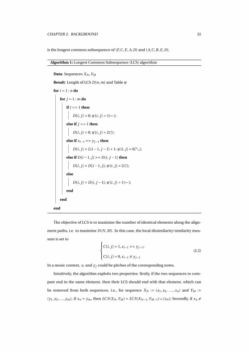
CHAPTER 2. BACKGROUND 32
is the longest common subsequence of {F,C ,E , A,D} and {A,C ,B ,E ,D}.
Algorithm 1: Longest Common Subsequence (LCS) algorithm
Data: Sequences XN ,YM
Result: Length of LCS D[n,m] and Table ψ
for i = 1 : n do
for j = 1 : m do
if i == 1 then
D[i , j ] = 0; ψ[i , j ] = 1(←);
else if j == 1 then
D[i , j ] = 0; ψ[i , j ] = 2(↑);
else if xi−1 == y j−1 then
D[i , j ] = L[i −1, j −1]+1; ψ[i , j ] = 0(↖);
else if D[i −1, j ] >= D[i , j −1] then
D[i , j ] = D[i −1, j ]; ψ[i , j ] = 2(↑);
else
D[i , j ] = D[i , j −1]; ψ[i , j ] = 1(←);
end
end
end
The objective of LCS is to maximise the number of identical elements along the align-
ment paths, i.e. to maximise D(N , M). In this case, the local dissimilarity/similarity mea-
sure is set to C [i , j ] = 1, xi−1 == y j−1;
C [i , j ] = 0, xi−1 6= y j−1
(2.2)
In a music context, xi and y j could be pitches of the corresponding notes.
Intuitively, the algorithm exploits two properties: firstly, if the two sequences to com-
pare end in the same element, then their LCS should end with that element, which can
be removed from both sequences, i.e., for sequence XN := (x1, x2, . . . , xn) and YM :=(y1, y2, . . . , ym), if xn = ym , then LC S(XN ,YM ) = LC S(XN−1,YM−1)∪ (xn); Secondly, if xn 6=

CHAPTER 2. BACKGROUND 33
ym , then LC S(XN ,YM ) is the longer one of LC S(XN−1,YM ) and LC S(XN ,YM−1). Therefore
we can break down the LCS problem into sub-problems and use dynamic programming
to build the solution in a bottom-up fashion, as shown in Algorithm 1.
By tracing back the Table T obtained by Algorithm 1, the Longest Common Subse-
quence can be derived easily, see an example in in Table 2.1.
As a strict matching algorithm where the local similarity measure is binary, LCS is of-
ten applied to file comparison and biological sequence analysis tasks. In a music context,
it is mainly used to align symbolic representations, such as score and performance data
in MIDI format.
y j F C E A D
xi 0 ← 0 ← 0 ← 0 ← 0 ← 0
A↑ ↑ ↑ ↑ ↖0 0 0 0 1 ← 1
C↑ ↑ ↖ ↑ ↑0 0 1 ← 1 1 1
B↑ ↑ ↑ ↑ ↑ ↑0 0 1 1 1 1
E↑ ↑ ↑ ↖0 0 1 2 ← 2 ← 2
D↑ ↑ ↑ ↑ ↑ ↖0 0 1 2 2 3
Table 2.1: An example of LCS alignment
2.3.1.2 Needleman-Wunsch (NW)
The Needleman-Wunsch algorithm (NW) (Needleman and Wunsch, 1970) was one of the
first dynamic programming algorithms to align biological sequences. Unlike LCS, it al-
lows matching non-identical elements which are biologically meaningful to be matched
together. Therefore the local similarity measure is not simply binary, instead, derived
by the evolutionary relationship of the biological sequences. It also introduces the con-
cept of "gap", which refers to the insertions and deletions in a sequence, which cannot
be matched with any elements in another sequence. Gaps are usually penalised with a

CHAPTER 2. BACKGROUND 34
constant cost d . Therefore, the total similarity matrix in Equation 2.1 is rewritten as
D(n,m) := max
D(n −1,m −1)+C (n,m),ψ[n,m] = 0(↖);
D(n −1,m)−d ,ψ[n,m] = 1(←);
D(n,m −1)−d ,ψ[n,m] = 2(↑)
(2.3)
In a music context, the Needleman-Wunsch algorithm is adapted in (Grachten et al.,
2013) to align recordings with structural differences by adding a penalty to skipping in the
alignment.
2.3.1.3 Dynamic Time Warping (DTW)
Dynamic time warping specialises in aligning temporal sequences. It has been well re-
searched as a tool to compare different speech patterns in the speech recognition com-
munity since the 1970s (Itakura, 1975; Rabiner and Juang, 1993). Later in 2001, it was in-
troduced for music alignment (Orio and Schwarz, 2001) and various extensions have been
proposed over the years. This section will introduce the concept of DTW firstly and skim
through some prominent extensions. For a comprehensive tutorial on DTW, see Chapter
4 of (Müller, 2007).
Basic algorithm
As the name suggests, Dynamic Time Warping compares sequences which are considered
to be a non-linear "warp" of each other in the time dimension. The algorithm aims at
finding a so called warping path that maps each time position in one version to the cor-
responding one in the other version. Therefore it can be used to measure the similarity
of time series independently of non-linear variations in the time dimension. It has been
applied in analysing various time series, including video, audio and graphics data.
In a music alignment context, the objective of DTW is to obtain an optimal alignment
minimising the total dissimilarity along the path p. The feature space F typically denotes
the space of normalised chroma features, the local cost measure c is usually a cosine (or
Euclidean) distance with weights set to (w1, w2, w3) = (2,1,1) to remove a bias for the di-
agonal direction (Dannenberg and Raphael, 2006; Dixon and Widmer, 2005). An example

CHAPTER 2. BACKGROUND 35
(a) CENS features for the performance of Milosz Magin
(b) CENS features for the performance of Gabor Csalog
(c) Cost matrix and Alignment path
Figure 2.4: An example of DTW alignment for two performance excerpts of Chopin Op. 24No.2
of aligning two audio performance excerpts with DTW is shown in Figure 2.4, where the
cosine distance c(xn , ym) = 1− ⟨xn ,ym⟩‖xn‖‖ym‖ is used.
Same as NW, DTW also allows non-identical matches. It also allows the map from one
to many, therefore there is no "gap" concept in DTW. That is because DTW is designed for
time series and it assumes the main local difference comes from tempo, where one fea-
ture of one version could be time-stretched to several features in another version. NW is
designed for biological sequences where the main local difference comes from mutation,
therefore insertion and deletion are penalised.
Extensions to Lower the Running Time
Since the cumulative cost matrix D is of size N∗M , the complexity of basic DTW algorithm
is quadratic, i.e. is in O(N M). Often, this is too high to be of practical use when aligning
features with a high temporal resolution or recordings having a long duration. Several
strategies have been proposed to make DTW-based methods more efficient. A straight-
forward way to reduce the search space is to use a constant global constraint region, such
as the Sakoe-Chiba (Sakoe and Chiba, 1978) bound or the Itakura parallelogram (Itakura,
1975). They force the alignment path to be within a fixed distance from the main diagonal
of the cumulative cost matrix. However, sometimes the optimal alignment may lie outside

CHAPTER 2. BACKGROUND 36
(a) (b) (c) (d)
Figure 2.5: Multiscale DTW: The alignment path (in white dot) is computed in one leveland projected to next level to construct the constraint (non-black region); The entries out-side the constraint is not computed (black region); From (a) to (d), the feature resolutionis increasing.
such global constraint. Later work proposed several strategies for more adaptive global or
local constraints (Müller et al., 2006; Salvador and Chan, 2004; Prätzlich et al., 2016; Dixon
and Widmer, 2005; Macrae and Dixon, 2010).
In particular, later chapters incorporate methods described in (Müller et al., 2006; Sal-
vador and Chan, 2004), referred to as multiscale DTW (FastDTW). The general idea is to
first compute a rough alignment at a low temporal resolution, which is then used to con-
strain the alignment process at higher resolutions, illustrated in Figure 2.5. This way, in
the cost matrix C and accumulative cost matrix D , only entries around the projected path
need to be computed. As shown in (Müller et al., 2006), this strategy is particularly useful
for music due to the high temporal correlation between neighbouring feature vectors, i.e.
the temporal feature resolution can be decreased without losing the information neces-
sary to find the correct path on the coarser level. In practise, it typically leads to a drop in
runtime by up to a factor of 30.
Extensions for Realtime Alignment
Many other techniques not only accelerate but enable a method to align sequences online
or in real-time. For example, the method presented in (Dixon and Widmer, 2005) employs
a greedy, locally optimal forward path estimation algorithm to constrain the alignment
path, while (Macrae and Dixon, 2010) employs a windowed variant of DTW integrating
ideas of the A∗ algorithm (Hart et al., 1968) to dynamic programming.
Extensions to Account for Structural Differences
Some extensions of DTW aim at addressing structural differences, i.e. the situation when

CHAPTER 2. BACKGROUND 37
musicians unexpectedly choose to repeat or skip an entire section. The method proposed
in (Arzt et al., 2008) caters for different choices musicians make in real-time by maintain-
ing multiple alignment instances. For off-line cases, (Fremerey et al., 2010) extends the
step size of DTW to include jumps between sections. (Müller and Appelt, 2008) analyses
the cost matrix between two versions before alignment and extract partial matches from
the alignment path.
2.3.1.4 Other Dynamic Programming Methods
There are some other dynamic programming based methods that have been applied to
music alignment. For example, the Smith-Waterman algorithm (Smith and Waterman,
1981) is a common local alignment method for biological sequence analysis and it was
used in (Ewert et al., 2009a) for partial alignment in the case of structural differences.
2.3.2 Probabilistic Modelling
It is natural to use dynamic programming if we think of finding the alignment path as an
optimisation problem. However, we could also interpret the task as a latent state estima-
tion problem by considering the pattern shared by all versions of a piece of music as the
latent/hidden states, while their feature sequences are our observations emitted from the
latent states. Following this train of thought, many probabilistic modelling methods have
been applied to the music alignment task. The following sections will introduce a widely
used and extended probabilistic modelling method, the Hidden Markov Model (HMM).
2.3.2.1 Hidden Markov Model (HMM)
This section will give a brief introduction to the standard Hidden Markov Model (HMM).
For more details, see tutorials of HMM (Rabiner, 1989; Stamp, 2004) .
As the name suggests, an HMM models a system which is assumed to be a Markov
process with hidden states. A Markov process is a stochastic process with the so called
Markov property, which we will see in more detail below. In a signal processing context,
a stochastic process is a system that evolves with time. The evolution in time is modelled
by the transitions between states. The Markov property regulates that the transition prob-
ability from the current state to the next state only depends on the current state and not

CHAPTER 2. BACKGROUND 38
on the past states. In an HMM, the states are hidden and can be observed only by the
random variables they emit according to certain probability distributions. To describe an
HMM model, the following notation is used:
L ← number of states;
S = (s1, s2, . . . , sL) ← states in the model;
N ← length of the observation sequence;
O = (O1,O2, . . . ,ON ) ← observation sequence;
ai j ← state transition probability from si to s j ;
π← initial state distribution;
bi (On) ← observation probability
In a music alignment context, the observation On is usually a feature vector, emitted by
state si with a certain probability distribution bi (On). The observation probability distri-
bution could either be discrete or continuous and here a continuous normal distribution
is discussed which is often used for time series,
bi (On) =N (On ;µi ,σ2i ) (2.4)
Figure. 2.6 shows an example HMM with a fully connected (ergodic) topology, meaning
every state can be reached from any state in a finite number of steps. There are other
types of topologies, such as a left-right HMM which only allows transition from left to
right, i.e. ai j = 0, j < i . It is often used when the number of states is relatively large or
avoid impractical or even infeasible parameter estimations.
An HMM can be applied to solve two problems in the music alignment task: decoding
and training. Decoding an alignment is to find the state sequence X := {x1, · · · , xN }, xi ⊂ S,
for i = 1, · · · , N , which is most likely to generate the given observation sequence O. Train-
ing is to adjust the parameters of the model λ = (a,b,π), so that it can best describe, or
maximise the probability of generating the observation sequences. The following will in-
troduce Viterbi decoding and Baum-Welch Traning for these two purposes.
Viterbi Decoding To find the best matched state sequence is an optimisation problem,
which can be solved with Dynamic Programming in the same fashion as introduced be-
fore. Instead of minimising the total cost as in DTW, here the goal is to maximise the prob-

CHAPTER 2. BACKGROUND 39
Figure 2.6: An example of HMM model
ability P (X |O,λ) which is equivalent to maximising P (X ,O|λ). To do so, define δn( j ) =maxP (x1, x2, · · · , xn = j ,O1,O2, · · · ,On |λ), i.e. δn( j ) is the highest probability given the ob-
servation until frame n. It can be calculated recursively as δn( j ) = maxi
[δn−1(i )ai j ]·b j (On)
and the choice of each step is recorded in another matrix ψn( j ) = argmaxiδn−1(i )ai j . At
the end, the best matched state sequence can be obtained by tracing back ψ. This proce-
dure is called Viterbi decoding (Rabiner, 1989).
Baum-Welch Training The Baum-Welch algorithm is often used in parameter estima-
tion for HMMs. The main idea is to use the Expectation-Maximisation algorithm to
find the Maximum Likelihood estimate of the model parameters. It iteratively performs
three processes: the forward procedure, the backward procedure and the parameter re-
estimation. The forward procedure computes a forward variable αi (n), defined as the
probability of the partial observation sequence until frame n and state Si at frame n, given
the model λ:
αi (n) = P (O1,O2 · · ·On , xn = si |λ) (2.5)
After initialisation αi (1) = πi bi (O1), i = 1,2 · · ·L , one computes αi (n) for n = 2,3 · · ·N and
i = 1,2 · · ·L recursively:
αi (n) = [L∑
j=1αn−1( j )a j i ]bi (On) (2.6)

CHAPTER 2. BACKGROUND 40
while terminates at P (O|λ) = ∑Li=1αi (N ). P (O|λ) is the model likelihood that the Baum-
Welch algorithm aims to maximise and it is used to define the termination criterion for
the iterative parameter estimation.
The backward procedure computes a backward variable βi (n) in a similar way. βi (n)
is the probability of the partial sequence from time n +1 to the end, given state Si at time
n and the model λ:
βi (n) = P (On +1,On +2 · · ·ON |xn = si ,λ) (2.7)
After initialisation βi (N ) = 1, i = 1,2 · · ·L, one computes βi (n) for n = N −1, N −2 · · ·1 and
i = 1,2 · · ·L recursively:
βi (n) =N∑
j=1ai j bi (Ot+1)β j (n +1) (2.8)
To re-estimate the parameters, define ξn(i , j ) as the probability of being in the state si
at time t and transiting to s j at time t+1, given the model λ and the observation sequence
O:
ξn(i , j ) = P (xn = si , xn+1 = s j |λ,O), (2.9)
which can be computed with the forward and backward variables:
ξn(i , j ) = αi (n)ai j b j (On+1)β j (n +1)
P (O|λ), (2.10)
Also define γn(i ) as the probability of being in the state si at the frame n given the model
λ and the observation sequence O, which is the sum of ξn(i , j ) over j ,
γn(i ) =L∑
j=1ξn(i , j ), (2.11)
The re-estimation of A and π is computed as:
πi = (expected frequency of state si at frame n = 1) = γ1(i ) (2.12)
ai j =expected number of transition from si to s j
expected number of transition from state si=
∑N−1n=1 ξn(i , j )∑N−1
n=1 γn(i )(2.13)
When the normal distribution is used as the observation probability distribution, i.e.
bi (On) = f (On |µi ,σ2i ), the re-estimation of B is computed as:
µi =∑N
n=1γn(i ) ·On∑Nn=1γn(i )
(2.14)
σ2i =
∑Nn=1γn(i ) · (On −µi )2∑N
n=1γn(i )(2.15)

CHAPTER 2. BACKGROUND 41
For a more complicated probability density function, one could use a M-component
Gaussian mixture model,
bi (O) =M∑
m=1ci mN (O;µi m ,σ2
i m), (2.16)
where ci m is the mixture coefficient for mth mixture in state i , for more detail see (Ra-
biner, 1989). In summary, the Baum-Welch training follows:
• Initialisation: λ= (A,B ,π);
• Recurrence:
– Calculate αi (n) and βi (n) with the forward-backward procedure;
– Calculate ξn(i , j ) and γn(i ) ;
– Re-estimate the model λ= (A, B , π);
• Termination condition: the model likelihood P (O|λ) stops increasing or is larger
than some predefined threshold or the maximum number of iterations is exceeded.
Viterbi Training As an alternative to the Baum-Welch algorithm, one can also use
Viterbi training (Durbin et al., 1999) to train the HMM. It replaces the forward-backward
procedure with Viterbi decoding to get the most likely state sequence and uses it to re-
estimate the model parameters in every iteration. This way, instead of a soft value encod-
ing the probability of being in a certain state at a certain time frame, the Viterbi decoding
makes a hard choice and sets the probability of the state-time pair to 1 if it is on the most
probable path, and to 0 otherwise. Compared to Baum-Welch, it does not aim to max-
imise the model likelihood and therefore the estimated parameters may not be as good
as the ones obtained from the Baum-Welch algorithm. However, since the continuous
model likelihood is not computed, Viterbi training tends to converges much faster than
Baum-Welch training.
Numerical Issues Note that the above computation will easily run into numerical issues.
For example, for the forward variable, since the transition probability is usually smaller
than 1, after multiplication for i = 1,2 · · · ,L and n = 1,2 · · · , N , the value of αi (n) expo-
nentially approaches zeros. If the absolute value is even smaller than the computer can

CHAPTER 2. BACKGROUND 42
actually represent, the true value will be replaced by zero. The solution to this underflow
error is to scale variables. For each n, define a scaling coefficient cn ,
cn = 1∑Li=1αi (n)
(2.17)
The forward and backward variables are scaled as αi (n) = cn ·αi (n) and βi (n) = cn ·βi (n).
Furthermore, the logarithm of P (O|λ) is computed as log[P (O|λ)] = −∑Nn=1 logcn . The
parameter re=estimation keeps the same after replacing the αi (n) and βi (n) with αi (n)
and βi (n) respectively. For details of the derivation, see (Rabiner, 1989; Stamp, 2004).
Adaptation to Music Tasks As a statistical modelling method for sequence analysis, the
HMM has been widely applied in various fields such as finance and biological sequence
analysis as well as speech recognition. It was introduced in the context of music alignment
in (Raphael, 1998) and has been widely studied and extended in MIR since then (Orio and
Déchelle, 2001; Cont, 2006; Miotto et al., 2010; Cont, 2010).
The HMM and its variations have been particularly popular in score-to-audio align-
ment tasks, as here each state intuitively corresponds to a note or a constellation of con-
current notes as specified by the score (Raphael, 1998; Orio and Déchelle, 2001; Cont et al.,
2005), while other assumptions about the music can be captured in higher-level HMM
structures. For examples, high-level states might encode the current tempo (Raphael,
2004), or each note-state can be subdivided into attack-decay-release sub-states (or simi-
lar temporal evolutions). Such high level structures lead to hierarchical HMMs and semi-
Markov graphical models, or generalisations thereof such as Dynamic Bayesian Networks
(DBNs) (Cont, 2010; Maezawa et al., 2014). It should be noted that many of these more
advanced models can still be represented as a standard HMM.
HMM based music alignment usually can work in real-time. The model is trained of-
fline and alignment is performed using online decoding methods (Raphael, 1998; Orio
and Déchelle, 2001; Pardo and Birmingham, 2005). On the contrary, the method proposed
in (Cont, 2010) avoids the need for offline training by using an anticipatory forward prop-
agation algorithm for real-time inference. To account for structural differences, possible
repeats and jumps according to the score could be encoded into the model through mod-
ification to the transition function (Pardo and Birmingham, 2005). However, the method
proposed in (Pardo and Birmingham, 2005) is only for symbolic music alignment.

CHAPTER 2. BACKGROUND 43
2.3.2.2 Other Probabilistic Modelling Methods
There are many other probabilistic modelling methods employed by the MIR commu-
nity for music alignment. Even before the HMM was introduced, Grubb and Dannenberg
(1997) proposed a stochastic method which models the score position with a continuous
probability density function, avoiding the problem of discrete states in contrast to a stan-
dard HMM.
Recently, conditional random fields (CRFs) have been used for music synchronisation
(Joder et al., 2011). As an advantage, CRFs loosen several limitations of HMM-based meth-
ods in contrast to more general DP methods, e.g. DTW. In particular, their use of so-called
feature-functions generalises the notion of observation probability and thus enables mea-
suring distances between features in a more general way than HMMs allow.
Conceptually quite different from the above are state-space methods, where states
such as position or tempo are elements of a continuous space. Transitions between states
are modelled using transition functions that, applied to the current state, yield the next
one (Duan and Pardo, 2011). Depending on specific properties of the sources of noise
in the model, one typically uses parameter estimation methods based on the Kalman fil-
ter, particle filter or more general Monte-Carlo sampling methods (Montecchio and Cont,
2011a).
2.3.3 Similarity between Dynamic Time Warping and Hidden Markov Model
Among various alignment methods, the most often used and extended ones are DTW and
HMM. They belongs to the above mentioned two categories respectively, with one being
described as an optimisation and the other as a probabilistic inference problem.
However, there are many similarities between them from an algorithmic point of view.
In particular, under certain conditions, DTW is equivalent to a negative log-likelihood im-
plementation of an HMM using multivariate Gaussian distributions for the observations.
This is the case if a Euclidean distance is used to compare features and additive is used
instead of multiplicative weights are used for different step sizes. With these limitations,
the application of a logarithm transforms the HMM-likelihood from a product of proba-
bilities to a sum of log-probabilities, which for the case of a Gaussian takes the form of a
Euclidean distance. One can show that the result is equivalent to DTW by interpreting the

CHAPTER 2. BACKGROUND 44
features of one DTW sequence as HMM states, using the features as the mean of the cor-
responding Gaussians and adding some non-emitting states to model certain step sizes
– see (Rabiner, 1989; Cox, 1990) for some discussion. Furthermore, both the calculation
of an optimal alignment path in DTW and the decoding of the most probable path are
instances of dynamic programming.
2.3.4 Other Techniques used in Music Alignment
Non-negative Matrix Factorisation (NMF) is applied in (Niedermayer, 2009b) as a post-
processing step in score to audio alignment to refine the mapped note onset positions.
NMF will be introduced in detail in Chapter 5. Recently, neural networks have been used
in a few works (Dorfer et al., 2016a,b) to map short music audio snippets to the corre-
sponding image location of a scanned sheet score.
2.4 Exploiting Score Information using Alignment Techniques in MIR
In music information retrieval (MIR) research, musical knowledge is often exploited to
improve the performance of a system. The score, as a natural source of music information,
has been used for a variety of tasks. This section will provide an overview of MIR research
which exploits score information based on alignment techniques.
2.4.1 Score-informed Expressive Parameter Extraction
A large body of work employs score to audio alignment techniques as a foundation for
extracting expressive parameters from recorded music performances. Here, score to audio
alignment is used to identify the rough time boundaries (onsets and/or offsets) for each
score note in a given audio recording, which then provides guidance for analysing the
audio performance.
For example, Scheirer (1995) proposed a method which employs the score to extract
onset and offset timing as well as dynamics for each score note from audio recordings of
musical performances. In this method, the tempo estimator is updated based on a linear
regression model of matched pairs of past score notes and detected onsets. Based on the
estimated tempo, a search window is chosen to extract onset, offset as well as dynamics

CHAPTER 2. BACKGROUND 45
Figure 2.7: Non-Negative Matrix Factorisation (NMF)
for each score note by spectral analysis. Earis (2007) used a similar idea to extract onset
time and dynamics from expressive performances, in which the manually aligned score
constrains the search window of the onset detection. This idea is also exploited in (Nieder-
mayer and Widmer, 2010), where NMF is used to refine the note onset position after auto-
matically aligning the given audio recording to the corresponding score. To estimate note
intensities in a music recording, Ewert and Müller (2011) proposed a parametrised spec-
trogram model, which is initialised using the aligned score for each note event. The model
parameters are estimated iteratively to minimise a distance between the audio and model
spectrogram. Most recently, a framework is proposed (Abeßer et al., 2017) for analysing
the tuning, intonation, pitch modulation and dynamics in Jazz recordings. It is based on
a score-informed solo and accompaniment separation. The use of score information can
help achieve a high quality source separation for music and it has attracted much research
interest in recent years. The following section will discuss it in more detail.
2.4.2 Score-informed Source Separation
Separating individual music sources from a mixture audio signal is a challenging task.
Usually music is distributed in a stereo format, that is to say, when there are several instru-
ments playing simultaneously, the signals from more than one instrument will be mixed
in the same channel (by recording with a single microphone or mixing down several chan-
nels afterwards). To boost the performance of the separation, many works use score in-
formation to help identify and locate sound events in the corresponding audio recording.
For example, a commonly used source separation method is Non-Negative Matrix Fac-
torisation (NMF), which decomposes an input spectrogram into the product of two non-
negative matrices, one containing spectral template vectors and the other encoding the

CHAPTER 2. BACKGROUND 46
activity of each template over time, demonstrated in Figure 2.7. For more details on NMF,
see (Lee and Seung, 2000). Essentially, NMF is an unsupervised learning process which
is expected to learn a dictionary consisting of the spectral patterns for individual compo-
nents in the input signal. (An individual component could be one pitch played by one
instrument.) However, the objective function of NMF is to minimise the distance between
the input spectrogram and the one reconstructed by multiplying the spectral template
matrix and the activation matrix. Therefore it may not produce a useful decomposition
even if the distance reaches a minimum in the learning process. However, from a machine
learning perspective, NMF belongs to the group of generative models, which often employ
interpretable parameters and thus enable a direct way to incorporate prior knowledge and
adapt the method to specific acoustic conditions (Ozerov et al., 2012; Ewert and Sandler,
2016). One rich source of prior information to guide the NMF learning process is the score.
After aligning the score to the given audio recording, one knows for each time position in
the recording, which instruments and which notes are expected to sound. The pitch and
timbre information can be used to constrain the spectral patterns for each component,
while the timing information (note boundaries) allows constraining the corresponding
activities for each component. For a comprehensive overview, see (Ewert et al., 2014).
Score-informed source separation techniques have been applied to note-based au-
dio editing (Driedger et al., 2013), remixing and upmixing of stereo music (Woodruff
et al., 2006), instrument-wise equalisation (Itoyama et al., 2008) and singing voice sep-
aration (Chan et al., 2015). The idea of score-informed dictionary learning can be adapted
to automatic music transcription (AMT). For example, for piano transcription, the com-
ponents of the expected dictionary could be the 88 piano pitches. The concept of score
informed transcription will be briefly introduced next.
2.4.3 Score-informed Transcription
The goal of automatic music transcription (AMT) is to obtain a high-level symbolic rep-
resentation of a given audio recording. As a fundamental problem in music processing, a
wide range of approaches has been proposed over the years, see (Klapuri and Davy, 2006;
Christensen and Jakobsson, 2009; Benetos et al., 2013) for more comprehensive overviews.
For example, Yeh et al. (2010) proposed a joint pitch estimation method by progressively

CHAPTER 2. BACKGROUND 47
combining F0 candidates into pitch or note objects. Further, various probabilistic models
have been employed for AMT, such as a method using maximum a posteriori (MAP) esti-
mation (Emiya et al., 2010) or methods based on non-parametric Bayesian models (Yoshii
and Goto, 2012). Modelled as a classification or regression task, transcription has also
been addressed by several discriminatively trained methods, using support vector ma-
chines (Poliner and Ellis, 2007), convolutional neural networks (Marolt, 2004; Kelz et al.,
2016), deep belief networks (Nam et al., 2011) or recurrent neural networks (Böck and
Schedl, 2012; Sigtia et al., 2015).
Among the various approaches, most state-of-the-art AMT methods are based on
spectrogram factorisation techniques, such as Non-negative Matrix Factorisation (NMF)
or its probabilistic formulation, Probabilistic Latent Component Analysis (PLCA) – see
(Virtanen et al., 2015) for an overview. NMF was introduced into AMT by Smaragdis and
Brown (2003) and many variants have been proposed in recent years. One type of vari-
ants regularise the learning procedure by adding constraints to spectral templates so as
to enforce a harmonic structure (Vincent et al., 2010; Bertin et al., 2010), or constraints
for the activity matrix to enhance temporal continuity and sparsity properties (Virtanen,
2007). Other variants such as non-negative matrix deconvolution (NMD) (Smaragdis,
2004) employ, instead of individual spectral template vectors as used in NMF, entire
spectro-temporal blocks as templates, each modelling a part of an entire segment in a
time-frequency representation. Since these blocks have a fixed size, NMD has mainly been
used for drum sound separation and transcription (Roebel et al., 2015). Shift-invariant
PLCA enhances NMF’s capability to represent changes in fundamental frequency by ef-
fectively coupling the parameter estimation for those templates associated with a specific
musical pitch (Benetos and Dixon, 2012). Finally, Markov constraints can be used to ex-
press that non-stationary sounds can often be modelled a sequence of specific spectral
templates, where the order is modelled using a graphical model (Ozerov et al., 2009; Bene-
tos and Dixon, 2013; Ewert et al., 2015); as discussed in (Ewert and Sandler, 2016), this
approach is particularly useful for modelling a few concurrent speakers but leads to vari-
ous numerical issues when applied to highly polyphonic sounds such as piano recordings.
However, despite being researched for several decades, current AMT methods are still
inadequate for many applications and seem to have reached a plateau in performance.

CHAPTER 2. BACKGROUND 48
To boost the accuracy, some works exploit the availability of additional information, such
as annotations made by users for the recording under analysis (Kirchhoff et al., 2012), or
single note recordings giving more details about the instrument in use and the recording
conditions (Klapuri and Davy, 2006; Ewert and Sandler, 2016). Another particular type of
prior knowledge is a musical score. Given the goal of AMT, score information may look like
the output rather than the prior knowledge. However, some applications, such as music
tutoring or performance analysis, aim to identify differences between the performance
and the given score. In these cases, score information is often available and can readily be
exploited to improve the AMT system.
Score-informed transcription is a relatively new concept. Benetos et al. (2012) pro-
posed such an AMT system to reduce the number of falsely detected notes by transcribing
both the performance recording and a synthesised recording of the score. The system then
discards the notes detected in both recordings which are not actually on the score. It can
be considered as a post-processing step to correct the results of a standard AMT method.
In contrast, Chapter 5 presents a method that integrates the score information directly
into the dictionary learning process so that the obtained spectral patterns are tuned to
the specific recording. The idea is inspired by score-informed source separation, intro-
duced in the previous section. Since the dictionary is highly adapted to the given audio
recording, it eliminates the requirement of single note recordings, in contrast to (Benetos
et al., 2012).
2.5 Discussion
This chapter reviewed the literature on music alignment and score-informed MIR re-
search which applies the alignment techniques. For one piece of music, there are often
various versions, including different forms of musical score and multiple recordings of
musical performances. Music alignment provides a way to establish links between these
different versions. Specifically, the goal of music alignment is to map each temporal posi-
tion in one version to the corresponding positions in other versions of the same piece. Fea-
ture representations used in music alignment and the related work on alignment methods
were discussed.

CHAPTER 2. BACKGROUND 49
Thanks to the considerable amount of research efforts over the years, various align-
ment methods have been proposed and current methods have achieved high accuracy
in many cases. However, musicians can interpret a piece in diverse ways, which leads to
complex differences on a musical level between individual performances. Additionally,
the wide range of possible acoustic conditions adds another layer of complexity to the
music alignment task. If such differences are substantial, even state-of-the-art methods
may fail in identifying a correct alignment. This thesis aims to improve the robustness for
some of these cases by developing novel sequence models and alignment methods that
can make use of specific information available in music synchronisation scenarios. Chap-
ter 3 and Chapter 4 will propose two strategies of improving the alignment robustness in
different scenarios.
By applying music alignment techniques, the score information can be exploited to as-
sist various MIR tasks, including expressive parameter extraction, source separation and
automatic music transcription. For automatic music transcription (AMT), the accuracy
of current methods are inadequate for many applications. To boost the accuracy of AMT,
Chapter 5 will apply the alignment techniques to exploit the score information in the dic-
tionary learning process.

CH
AP
TE
R
3ROBUST JOINT ALIGNMENT OF MULTIPLE
PERFORMANCES
3.1 Introduction
Chapter 2 reviewed various methods for aligning different versions of a piece of music.
The goal of most of these methods is to map each temporal position in one version of
a piece of music to the corresponding position in another version. Such pairwise align-
ment methods achieve high accuracy in many cases (Joder et al., 2011; Ewert et al., 2009b;
Dixon and Widmer, 2005). However, even the state-of-art still often fails to identify a cor-
rect alignment if versions differ substantially with respect to acoustic conditions or mu-
sical interpretation. To increase the robustness for these cases, this chapter exploits the
availability of multiple versions of the piece to be aligned. By processing these jointly,
the alignment process can be stabilised with additional examples of how a musician can
realise a section of a piece or which acoustic conditions might prevail in a recording.
The chapter is arranged as follows. First, the motivation of this work is discussed in
Section 3.2. As the proposed methods are inspired by the multiple sequence alignment
methods as used in biology, related work and some necessary background is given in Sec-
tion 3.3. Two proposed joint alignment methods are described in Section 3.4, based on
50

CHAPTER 3. ROBUST JOINT ALIGNMENT OF MULTIPLE PERFORMANCES 51
Figure 3.1: Alignment of two interpretations of Chopin Op. 24 No. 2, measures 52-57: (a)Score for the six measures. (b)/(c) CENS features (a variant of chroma features proposed in(Müller et al., 2005)) for interpretations by Luisada and Richter, respectively. (d) Alignmentresults for the pairwise (solid), proposed progressive alignment (dashed) and profile HMM(dotted); ground truth are given as corresponding beat positions from the two versions(red).
progressive alignment and profile HMM respectively. Their differences and similarities
are discussed in Section 3.5. An in-depth analysis of the behaviour of both joint alignment
methods is provided in Section 3.6. A conclusion is given in Section 3.7.
3.2 Motivation
As shown in Chapter 2, the objective of pairwise alignment is to find an alignment path
along which the two versions match best or more precisely, to minimise the total dissimi-
larity between features from both versions, subject to some path constraints . However, a
musician can interpret a piece in diverse ways, which can lead to substantial local differ-
ences between versions in terms of articulation and note lengths, ornamental notes (grace
notes, trills), or the relative loudness of notes (balance). Additionally, there could also be
complex differences in the acoustic environment, instrumentation and recording condi-
tions. Those differences can reduce the alignment accuracy of state-of-the-art methods
drastically.
CHAPTER 3. ROBUST JOINT ALIGNMENT OF MULTIPLE PERFORMANCES 52
Figure 3.1 shows a real-world example of a pair-wise method failing to compute a cor-
rect alignment between two recordings of Chopin’s Op. 24 No. 2. Chroma features for
both recordings shown in Figure 3.1b and c reveal acoustical (more noise in the C] and D
chroma bands in Figure 3.1c) and musical differences (more pronounced staccato on the
E and G notes in Figure 3.1b). Since the piece shows a repetitive pattern on the chroma
level, such differences cause a pairwise method (Ewert et al., 2009b) to compute an incor-
rect alignment between the two versions. The results are shown in Figure 3.1d as a grey
alignment path, which encodes corresponding positions between the two recordings as
computed by the method – note how the path deviates from the correct positions between
57.5–61.5 seconds (in the timeline of Luisada’s version).
To improve the alignment accuracy for such difficult cases, this chapter exploits the
fact that in many cases not only two but multiple versions of a piece are available. This is
the case, for example, in comparative performance analysis (Widmer et al., 2003; Sapp,
2007; Müller et al., 2009) and expressivity studies (Liem and Hanjalic, 2011), in music
production where corresponding audio takes need to be aligned (Montecchio and Cont,
2011b), when coordinating user-generated videos of a concert (Basaran et al., 2015) or
generating ground-truth for large scale distance learning (Raffel and Ellis, 2015). If multi-
ple versions are indeed available, the idea is to align them in a joint way, which facilitates
the synchronisation process as every additional version presents another example of how
a musician can realise a section of a piece or which acoustic conditions might prevail in a
recording.
Instead of only aligning two versions with strong local differences, including other
available versions can help stabilising the alignment process. As a first indication, this is
illustrated in Figure 3.1d: the results computed using the proposed joint alignment meth-
ods are shown as two additional paths (dashed and dotted), in which the overall robust-
ness and alignment accuracy is increased considerably.
3.3 Background on Multiple Sequence Alignment
The straightforward idea to align multiple versions is to extend dynamic programming
techniques (reviewed in Chapter 2) to multiple dimensions so that several sequences can

CHAPTER 3. ROBUST JOINT ALIGNMENT OF MULTIPLE PERFORMANCES 53
be aligned jointly. Instead of constructing a two-dimensional look-up table as in Fig-
ure 2.3, a multi-dimensional table can be built to store solutions to all sub-problems.
This has been demonstrated in the context of gesture recognition (Holt et al., 2007) and
multi-modal speech recognition (Wöllmer et al., 2009). However, it is easy to spot that the
computational complexity of this strategy will increase exponentially with the number of
sequences. Assuming that each sequence to be aligned is roughly of length N , the time
and memory requirement to align K versions is O(N K ). Path pruning techniques can be
used to mitigate such problems for small values of K as shown in the next chapter of this
thesis. But in general for large K , it can be very difficult to lower the computational costs
enough to become practically feasible and find accurate alignments at the same time.
On the other hand, a joint synchronisation of music recordings can be considered
as an instance of the multiple sequence alignment problem, a task well-studied in bio-
informatics (Durbin et al., 1999; Gusfield, 1997). For example, the MAFFT (Katoh and
Standley, 2013) and CLUSTAL (Sievers et al., 2011) families of algorithms have been in
development for almost three decades. While a lot of the functionality in such packages
is highly specific to the alignment of biological sequences such as DNA or protein se-
quences, some central ideas can be adapted for the music alignment task, taking music
specific properties into account.
Most of the multiple sequence alignment algorithms fall into two classes, progressive
alignment (PA) methods and probabilistic profile (PP) methods. PA methods begin with
a pairwise alignment of the most similar sequences, and progressively include more se-
quences typically ordered in a suitable way according to their alignment difficulty. More
precisely, the alignment process follows a previously built "guide tree", which orders the
sequences by an efficient clustering method based on the pairwise alignment score for
each pair. PP methods , one the other hand, are typically based on Hidden Markov Models
(HMM), where the hidden states represent the ancestral sequence of the sequences to be
aligned. Every time a new sequence is processed, the model is updated and it influences
the alignment of all sequences. On the contrary, in PA methods, the alignments of prior
sequences are fixed and will remain the same even if new information arrives. The heuris-
tics of PA methods often lead to a considerably higher computational efficiency compared
to the PP methods. However, as reported by Pais et al. (2014), PP methods were found to

CHAPTER 3. ROBUST JOINT ALIGNMENT OF MULTIPLE PERFORMANCES 54
yield a higher alignment accuracy in some bioinformatics tasks.
Music recordings, however, have properties quite different from biological sequences.
First, this work does not consider structural differences between performances (e.g. a
section being left out in one version), which is in stark contrast to biological sequences
where such fundamental differences are common. Second, music recordings change
more slowly over time leading to a high temporal correlation between neighbouring se-
quence elements, which again is quite different from protein sequences. Due to these
differences, it is interesting to test whether the two types of methods can benefit the align-
ment accuracy in a musical context and how they differ in behaviour in such a scenario.
This work adapts these two types of multiple sequence alignment methods to the music
context and their detailed description is given in the next section.
With respect to musical applications, aligning multiple performances of a piece of
music is a relatively novel concept in music processing and has only been exploited by
a few approaches. A generative note duration model is proposed by (Maezawa et al.,
2015) that couples parameters associated with tempo curves from different performances.
Arzt and Widmer (2015) use multiple performances to improve the accuracy in an on-line
score-following application by computing several pairwise alignments in parallel. Further,
Bergomi (2015) aligns multiple symbolic sequences for harmonic and motivic analysis.
In some sense, the idea of using multiple versions to improve the performance of mu-
sic alignment is similar to the co-segmentation problem in computer vision, where the
segmentation accuracy can often be improved by supplying the algorithm with additional
images that share certain foreground characteristics with a given image and segmenting
them jointly (Rother et al., 2006). In addition, Müller and Röder (2006) proposed a method
to identify the related motion capture data in some database, by learning a motion tem-
plate from existing motion data sequences. A motion template is an average of align-
ments between each existing motion sequence with a reference motion sequence. In a
way, the template captures the essence of all the existing data sequences. It can help im-
prove the accuracy of identification and the robustness against the large variations among
the motion sequences. The main difference between it and the idea of this Chapter is that,
the proposed methods in this Chapter do not require choosing a reference sequence be-
forehand which may lead to some loss of robustness. Instead, as described below, a data

CHAPTER 3. ROBUST JOINT ALIGNMENT OF MULTIPLE PERFORMANCES 55
structure that represents the consensus of all the available sequences is built gradually as
sequences are processed.
3.4 Methods for Joint Music Alignment
Essentially, both PA and PP methods build up a data structure successively representing an
average sequence or central consensus against which all given sequences can be aligned.
In biological sequence analysis, the consensus sequence can be viewed as the common
ancestor from which all sequences are descended. In a musical context, constructing this
consensus form can incorporate information from every single recording such that the
overall alignment becomes easier (as the influence of outlier information can be reduced)
and therefore becomes more accurate and robust. In the following, two conceptually dif-
ferent methods are presented for computing such a central consensus in a music syn-
chronisation scenario. Their differences include how the central consensus is represented
(keeping all information in contrast to averaging some) and how it is built up (early versus
late updates). Both of these affect the resulting alignment accuracy and computational
performance, as discussed in more detail below.
3.4.1 Progressive Alignment
The first method can be regarded as a member of the family of progressive alignment (PA)
algorithms in the context of bioinformatics (Katoh and Standley, 2013) and it takes the
form of a general dynamic programming approach. The idea is, instead of simultane-
ously aligning all feature sequences, to successively add the sequences to a data structure
referred to as the template. The template comprises a set of feature sequences that are
aligned to each other. More precisely, after computing an alignment between a new se-
quence and the template at each step, the sequence is added using the alignment infor-
mation to stretch both the template and the sequence. The stretching step causes all the
feature sequences in the template to have the same length, which enables efficient access
to aligned sequence elements. This is repeated until all sequences are contained in the
template, which allows for deriving pairwise alignments between any two sequences.
To describe the alignment procedure in more detail, assume that there are K different
versions of a piece and that their feature sequences are denoted by X k = (xk1 , . . . , xk
Nk) with

CHAPTER 3. ROBUST JOINT ALIGNMENT OF MULTIPLE PERFORMANCES 56
k ∈[1 : K ] and xkn ∈ F , where F denotes a suitable feature space. Further, the template
data structure is refereed to as F and initialised to X 1. As part of the alignment process,
the remaining feature sequences X 2, . . . , X K are aligned successively to F , updating F af-
ter each step. To this end, let X k denote the sequence to be aligned and F = ( f1, . . . , fM )
the current template of length M . Each fm ∈ (F ∪ {G})k−1 contains k −1 elements which
are either feature vectors or gap symbols G , where individual components are denoted by
f 1m , . . . , f k−1
m ∈ F ∪ {G}. The idea behind the gap symbol will be discussed below. Further,
to simplify the notation later, the sequence ( f r1 , . . . , f r
M ) is denoted by F r for r ∈ 1, . . . ,k −1.
An alignment between F and X k is defined as a sequence p = (p1, . . . , pL) with p` =(m`,n`) ∈ [1 : M ]×[1 : Nk ] for ` ∈ [1 : L] satisfying 1 = m1 ≤ m2 ≤ . . . ≤ mL = M and 1 =n1 ≤ n2 ≤ . . . ≤ nL = Nk (boundary and monotonicity conditions), as well as p`+1 − p` ∈{(1,1), (1,0), (0,1)} (step size condition). To compute an alignment p between F and X k , a
cost matrix C r ∈RM×Nk comparing each pair of elements in F r and X k is computed by:
C r (m,n) =
c( f r
m , xkn), f r
m 6=G ,
CG , f rm =G ,
(3.1)
where c : F×F →R is a suitable dissimilarity measure between feature vectors and CG > 0
is a constant referred to as the gap penalty. By combining these individual cost matrices
C r to a merged cost matrix C ∈ RM×Nk , a dissimilarity measure is obtained between every
sequence element in F and X k . A simple yet effective combination is averaging:
C (m,n) = 1
k −1
k−1∑r=1
C r (m,n). (3.2)
This process is illustrated with an example of aligning five synthetic recordings in
Figure 3.2, where a template (Figure 3.2a) containing four sequences of chroma-based
vectors (with yellow entries indicating gap symbols) is aligned to a fifth sequence (Fig-
ure 3.2b). The resulting four cost matrices C 1 to C 4 are shown in Figure 3.2c-f, using CG = 3
and a cosine distance c( f , x) = 2− ⟨ f ,x⟩‖ f ‖‖x‖
1. The resulting merged cost matrix C is shown
in Figure 3.2g.
By combining the information provided by each individual cost matrix, the influence
of strong local differences on the alignment, that often only occur between specific pairs of
1Here a constant 1 is added to the cosine distance, in order to make the distance of chroma-based featurescomparable with the Euclidean distance of DLNCO features, mentioned in 3.5.1.3.
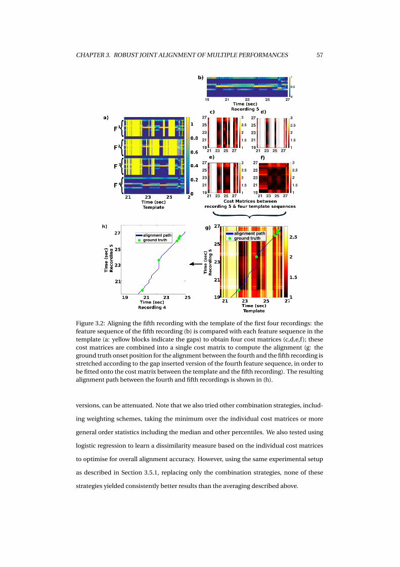
CHAPTER 3. ROBUST JOINT ALIGNMENT OF MULTIPLE PERFORMANCES 57
Figure 3.2: Aligning the fifth recording with the template of the first four recordings: thefeature sequence of the fifth recording (b) is compared with each feature sequence in thetemplate (a: yellow blocks indicate the gaps) to obtain four cost matrices (c,d,e,f); thesecost matrices are combined into a single cost matrix to compute the alignment (g: theground truth onset position for the alignment between the fourth and the fifth recording isstretched according to the gap inserted version of the fourth feature sequence, in order tobe fitted onto the cost matrix between the template and the fifth recording). The resultingalignment path between the fourth and fifth recordings is shown in (h).
versions, can be attenuated. Note that we also tried other combination strategies, includ-
ing weighting schemes, taking the minimum over the individual cost matrices or more
general order statistics including the median and other percentiles. We also tested using
logistic regression to learn a dissimilarity measure based on the individual cost matrices
to optimise for overall alignment accuracy. However, using the same experimental setup
as described in Section 3.5.1, replacing only the combination strategies, none of these
strategies yielded consistently better results than the averaging described above.
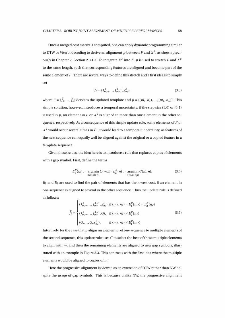
CHAPTER 3. ROBUST JOINT ALIGNMENT OF MULTIPLE PERFORMANCES 58
Once a merged cost matrix is computed, one can apply dynamic programming similar
to DTW or Viterbi decoding to derive an alignment p between F and X k , as shown previ-
ously in Chapter 2, Section 2.3.1.3. To integrate X k into F , p is used to stretch F and X k
to the same length, such that corresponding features are aligned and become part of the
same element of F . There are several ways to define this stretch and a first idea is to simply
set
f` = ( f 1m`
, . . . , f k−1m`
, xkn` ), (3.3)
where F = ( f1, . . . , fL) denotes the updated template and p = ((m1,n1), . . . , (mL ,nL)
). This
simple solution, however, introduces a temporal uncertainty: if the step size (1,0) or (0,1)
is used in p, an element in F or X k is aligned to more than one element in the other se-
quence, respectively. As a consequence of this simple update rule, some elements of F or
X k would occur several times in F . It would lead to a temporal uncertainty, as features of
the next sequence can equally well be aligned against the original or a copied feature in a
template sequence.
Given these issues, the idea here is to introduce a rule that replaces copies of elements
with a gap symbol. First, define the terms
E p1 (m) := argmin
{(m,n)∈p}C (m, n),E p
2 (n) := argmin{(m,n)∈p}
C (m,n). (3.4)
E1 and E2 are used to find the pair of elements that has the lowest cost, if an element in
one sequence is aligned to several in the other sequence. Thus the update rule is defined
as follows:
f` =
( f 1m`
, . . . , f k−1m`
, xkn` ), if (m`,n`) = E p
1 (m`) = E p2 (n`)
( f 1m`
, . . . , f k−1m`
,G), if (m`,n`) 6= E p2 (n`)
(G , . . . ,G , xkn` ), if (m`,n`) 6= E p
1 (m`)
(3.5)
Intuitively, for the case that p aligns an element m of one sequence to multiple elements of
the second sequence, this update rule uses C to select the best of these multiple elements
to align with m, and then the remaining elements are aligned to new gap symbols, illus-
trated with an example in Figure 3.3. This contrasts with the first idea where the multiple
elements would be aligned to copies of m.
Here the progressive alignment is viewed as an extension of DTW rather than NW de-
spite the usage of gap symbols. This is because unlike NW, the progressive alignment

CHAPTER 3. ROBUST JOINT ALIGNMENT OF MULTIPLE PERFORMANCES 59
Figure 3.3: An example of replacing copies of elements with gap symbols after aligning anew sequence X to the template F , where C (3,2) <C (2,2) and C (5,5) <C (5,4).
procedure does not open gaps when computing an alignment. Instead, gaps are opened
when integrating the newly aligned sequence X k into F according to the computed align-
ment path at each step. This way, the algorithm will not penalise the tempo difference
when computing an alignment. Rather, the gap is used when updating F , in order to avoid
temporal uncertainty in aligning the remaining sequences.
The importance of the gap symbol will be investigated in Section 3.6.2. Also, the order
in which feature sequences are aligned is crucial to the PA method and will be discussed
in Section 3.6.3.
3.4.2 Probabilistic Profile
Another central class of multiple sequence alignment methods are probabilistic profile
(PP) methods. For these methods, the central consensus data structure takes the form of a
Hidden Markov Model (HMM), in a specific configuration. Such a Profile HMM is adapted
to the music synchronisation scenario in the following; see also (Durbin et al., 1999) for
similar concepts used in bio-informatics.
The topology of the proposed profile HMM is illustrated in Figure 3.4. Overall, the
model contains three different types of states: Match states (M), Insert states (I) and Delete
states (D). Intuitively, the series of match states will encode the core of a consensus se-
quence representing the commonalities among different recordings, while the insert and
delete states are used to model the temporal diversity. To find appropriate parameters
for the various probability distributions involved, each given sequence is interpreted as
a noisy observation of the consensus sequence with insertions and deletions, and thus
can be used to train the model using a Baum-Welch procedure. Interpreted in this way, it
should be noted that the match states do not necessarily correspond to musical events like

CHAPTER 3. ROBUST JOINT ALIGNMENT OF MULTIPLE PERFORMANCES 60
Figure 3.4: Topology of a Profile HMM (Durbin et al., 1999), showing rows of delete states (top),insert states (middle) and match states (bottom)
specific chords or note constellations as specified by a score. Our goal is to train the model
using the given sequences, such that the final model captures a statistical description of
the consensus as well as the diversity among multiple versions, which provide a higher
robustness against large local discrepancies when the alignment for each pair is inferred
from the model.
To describe the model in more detail, the same notation as above is employed, i.e.
K different versions of a piece are assumed to be given with corresponding feature se-
quences denoted by X k = (xk1 , . . . , xk
Nk) for k ∈[1 : K ], where each xk
n ∈ F . Some general
concepts are similar to the standard HMM, which was described in Chapter 2. To de-
fine the structure of the profile HMM, the first step is to choose the length L of model:
The number of M and D states is L, respectively, while there are L + 1 I-states, com-
pare Figure 3.4. Note that L is the length of the model, not the length of a decoded se-
quence. Although L could simply be a constant (as often used in bio-informatics), ex-
periments described in the following sections show that the best results are obtained
by adapting L to the length of the given feature sequences. More precisely, it is set to
L = median(N1, . . . , NK ), which fixes the overall topology, shown in Figure 3.4. Compared
to other alternatives including the minimum, maximum and twice the maximum, the me-
dian led to a higher overall alignment accuracy in the experiments.
From a generative point of view, we start from a non-emitting Begin state. This way,
the first features of sequences are not forced to align together. From there we can enter
the first match state, the first insert state or the first delete state. If we enter the first match
state, we can draw a feature vector according to the corresponding observation probabil-
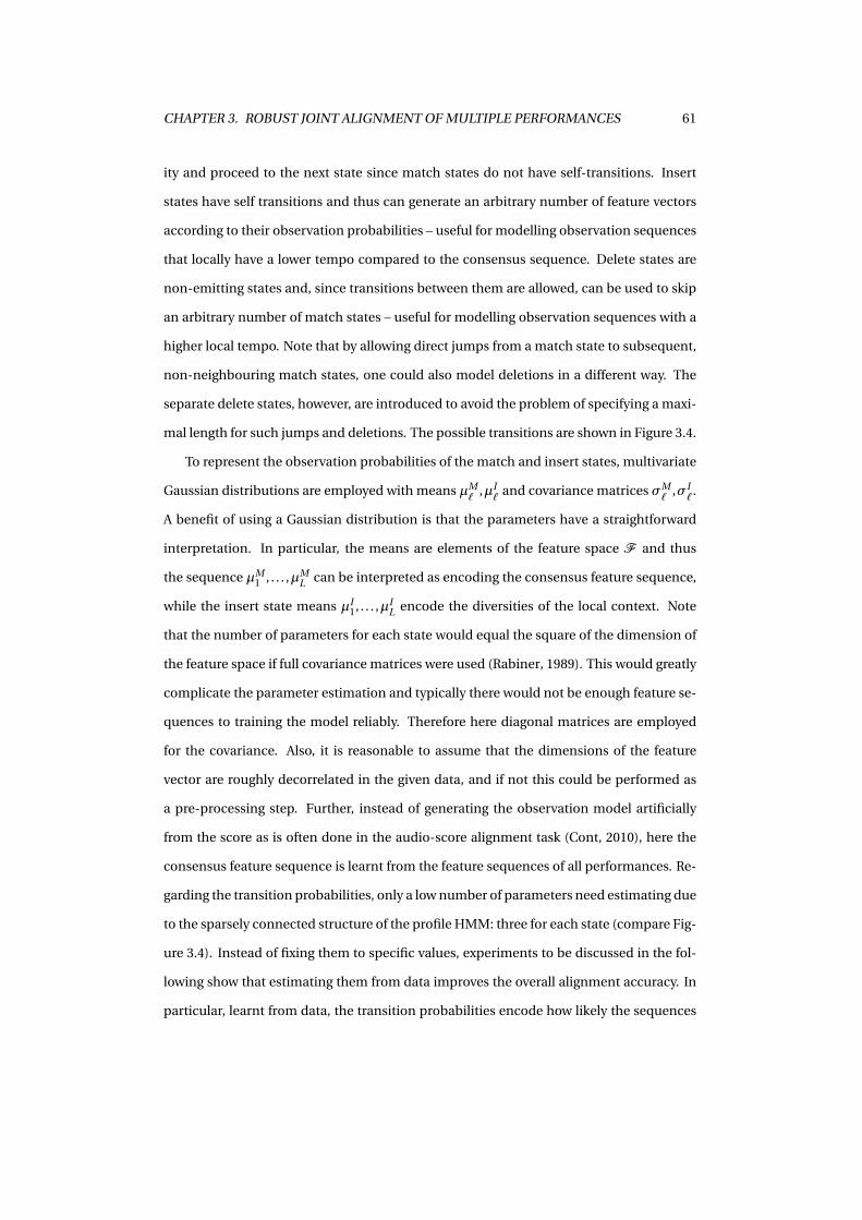
CHAPTER 3. ROBUST JOINT ALIGNMENT OF MULTIPLE PERFORMANCES 61
ity and proceed to the next state since match states do not have self-transitions. Insert
states have self transitions and thus can generate an arbitrary number of feature vectors
according to their observation probabilities – useful for modelling observation sequences
that locally have a lower tempo compared to the consensus sequence. Delete states are
non-emitting states and, since transitions between them are allowed, can be used to skip
an arbitrary number of match states – useful for modelling observation sequences with a
higher local tempo. Note that by allowing direct jumps from a match state to subsequent,
non-neighbouring match states, one could also model deletions in a different way. The
separate delete states, however, are introduced to avoid the problem of specifying a maxi-
mal length for such jumps and deletions. The possible transitions are shown in Figure 3.4.
To represent the observation probabilities of the match and insert states, multivariate
Gaussian distributions are employed with means µM`
,µI`
and covariance matrices σM`
,σI`
.
A benefit of using a Gaussian distribution is that the parameters have a straightforward
interpretation. In particular, the means are elements of the feature space F and thus
the sequence µM1 , . . . ,µM
L can be interpreted as encoding the consensus feature sequence,
while the insert state means µI1, . . . ,µI
L encode the diversities of the local context. Note
that the number of parameters for each state would equal the square of the dimension of
the feature space if full covariance matrices were used (Rabiner, 1989). This would greatly
complicate the parameter estimation and typically there would not be enough feature se-
quences to training the model reliably. Therefore here diagonal matrices are employed
for the covariance. Also, it is reasonable to assume that the dimensions of the feature
vector are roughly decorrelated in the given data, and if not this could be performed as
a pre-processing step. Further, instead of generating the observation model artificially
from the score as is often done in the audio-score alignment task (Cont, 2010), here the
consensus feature sequence is learnt from the feature sequences of all performances. Re-
garding the transition probabilities, only a low number of parameters need estimating due
to the sparsely connected structure of the profile HMM: three for each state (compare Fig-
ure 3.4). Instead of fixing them to specific values, experiments to be discussed in the fol-
lowing show that estimating them from data improves the overall alignment accuracy. In
particular, learnt from data, the transition probabilities encode how likely the sequences

CHAPTER 3. ROBUST JOINT ALIGNMENT OF MULTIPLE PERFORMANCES 62
are to deviate from the consensus sequence locally, thus provide additional guidance dur-
ing the alignment process.
Parameters of the model are estimated using a multiple sequence variant of the Baum-
Welch algorithm (Rabiner, 1989). The algorithm is similar to the Profile HMM used in the
biological sequence analysis (Durbin et al., 1999), for completeness of the discussion, it is
specified as below.
Firstly, the forward algorithm is adjusted according to the topology of the model. Un-
like the basic algorithm, here we have three forward variables, αMl (n), αIl (n), αDl (n), cor-
responding to three types of states, where αMl (n) represents the probability of the partial
observation sequence until state Ml at the feature frame n, given the model λ (αIl (n) and
αDl (n) are defined similarly). Let the first non-emitting Begin state be M0. The forward
variable is initialised as αM0 (0) = 1. The recursion steps to compute forward variables at
feature frames n = 1,2 · · ·Nk are:
αMl (n) = bMl (xn)[αMl−1 (n −1)aMl−1Ml +αIl−1 (n −1)aIl−1Ml +αDl−1 (n −1)aDl−1Ml ] (3.6)
αIl (n) = bIl (xn)[αMl (n −1)aMl Il +αIl (n −1)aIl Il +αDl (n −1)aDl Il ] (3.7)
αDl (n) =αMl−1 (n)aMl−1Dl +αIl−1 (n)aIl−1Dl +αDl−1 (n)aDl−1Dl (3.8)
where b represents the emission probability and a represents the transition probability.
The forward variable of the first insertion state is defined as αI0 (n) = bI0 (xn)aM0 I0 , while
the forward variable of the first delete state is defined as αD1 (n) = aM0D1 . The above re-
cursion steps terminate at the End state, defined as ML+1, where P (X |λ) =αML+1 (N +1) =αML (N )aML ML+1 +αIL (N )aIL ML+1 +αDL (N )aDL ML+1 .
Similarly, the backward algorithm is initialised as βML+1 (N +1) = 1 and the recursion
steps at the feature frames N , N −1 · · · ,0 are:
βMl (n) = bMl+1 (xn+1)βMl+1 (n +1)aMl Ml+1 +bIl (xn+1)βIl (n +1)aMl Il +βDl+1 (n)aMl Dl+1
(3.9)
βIl (n) = bMl+1 (xn+1)βMl+1 (n +1)aIl Ml+1 +bIl (xn+1)βIl (n +1)aIl Il +βDl+1 (n)aIl Dl+1
(3.10)
βDl (n) = bMl+1 (xn+1)βMl+1 (n +1)aDl Ml+1 +bIl (xn+1)βIl (n +1)aDl Il +βDl+1 (n)aDl Dl+1
(3.11)

CHAPTER 3. ROBUST JOINT ALIGNMENT OF MULTIPLE PERFORMANCES 63
To avoid the numerical issues mentioned in 2.3.2.1, the actual implementation com-
putes the above equations in the log domain. The forward and backward variables are
computed for each sequence. As mentioned in 2.3.2.1, the Baum-Welch training proce-
dure uses the Expectation-Maximisation algorithm. That is to say, the expectations are
calculated for each sequence and the maximisation step is performed on the accumu-
lated expectations of all sequences. The steps to re-estimate the model parameters are
specified as the following: Let the expected number of transition from state Sl : Ml , Il ,Dl
to state Ml+1,Il and Dl+1 for all sequences be ESl Ml+1 , ESl Il and ESl Dl+1 respectively, com-
puted as:
ESl Ml+1 =K∑k
1
P (X k |λ)
Nk∑n
bMl+1 (xkn+1)αk
Sl(n)βk
Ml+1(n +1)aSl Ml+1 (3.12)
ESl Il =K∑k
1
P (X k |λ)
Nk∑n
bIl (xkn+1)αk
Sl(n)βk
Il(n +1)aSl Il (3.13)
ESl Dl+1 =K∑k
1
P (X k |λ)
Nk∑nαk
Sl(n)βk
Dl+1(n)aSl Dl+1 (3.14)
The transition probabilities are then computed as:
aSl Ml+1 =ESl Ml+1
ESl Ml+1 +ESl Il +ESl Dl+1
(3.15)
aSl Il =ESl Il
ESl Ml+1 +ESl Il +ESl Dl+1
(3.16)
aSl Dl+1 =ESl Dl+1
ESl Ml+1 +ESl Il +ESl Dl+1
(3.17)
To re-estimate the means and covariance matrices of the observation probabilities,
the probability of being in the state Sl at the feature frame n given the model λ and the
observation sequence X k is represented by,
γkSl
(n) =αk
Sl(n)βk
Sl(i )
P (X k |λ)(3.18)
The means are computed as:
µMl =
∑Kk=1
∑Nkn=0γ
kMl
(n)xkn∑K
k=1
∑Nkn=0γ
kMl
(n)(3.19)
µIl =
∑Kk=1
∑Nkn=0γ
kIl
(n)xkn∑K
k=1
∑Nkn=0γ
kIl
(n)(3.20)

CHAPTER 3. ROBUST JOINT ALIGNMENT OF MULTIPLE PERFORMANCES 64
The covariances are computed as:
σMl =
∑Kk
∑Nkn γk
Ml(n)(xk
n −µMl )2∑K
k
∑Nkn γk
Ml(n)
(3.21)
σIl =
∑Kk
∑Nkn γk
Il(n)(xk
n −µIl )2∑K
k
∑Nkn γk
Il(n)
(3.22)
The multiple sequence variant of the Baum-Welch algorithm is summarised in Algo-
rithm 2:
Algorithm 2: A Multiple Sequence Variant of the Baum-Welch Algorithm
Data: Sequences X 1, X 2, · · ·X K
Result: New model parameters
Initialise the model parameters
repeat
for each sequence X k , k = 1,2 · · ·K do
Calculate the forward variable αkSl
(n) with Equations 3.6-3.8
Calculate the backward variable βkSl
(n) with Equations 3.9-3.11
Calculate γkSl
(n) with Equation 3.18
end
Re-estimate the model parameters with Equations 3.12-3.22
until the likelihood of the model∏K
k P (X k |λ) stops increasing or is larger than the
threshold or the maximum number of iterations is exceeded;
Since in a music synchronisation scenario the number of available sequences is typi-
cally several orders of magnitude smaller than in bioinformatics, the initialisation strategy
is crucial to avoid running into poor local maxima of the likelihood function. The highest
alignment accuracies are obtained using the following initialisation strategy: the match
and insert means are initialised using the feature vectors of a sequence whose length is
equal to the above chosen L. Excluding that sequence from the training procedure enables
the model to properly account for the other sequences without overfitting the initialising
sequence. Other strategies to obtain a proper initialisation led to lower alignment accu-
racies, including random initialisations as well as resampling all sequences to the same
length (corresponding to a linear stretch), followed by averaging. The covariance matrices

CHAPTER 3. ROBUST JOINT ALIGNMENT OF MULTIPLE PERFORMANCES 65
Figure 3.5: Emission probability matrices for match states with alignment path (blue) be-tween states and observations of (a) the fourth recording and (b) the fifth recording. Thevalues on colour bar are in log scale. Note that the extremely low probabilities (white area)on the top left and the bottom right corner result from the path constraint described inSection 3.4.3; (c) The resulting alignment path between the fourth and fifth recordings.
were uniformly initialised to a fixed, relatively high value as a measure to overcome over-
fitting. Additionally, to avoid the collapsing-Gaussian problem, the estimated variances
are constrained to a reasonable minimum (Durbin et al., 1999). The transition proba-
bilities were initialised uniformly, with the exception of match-match and delete-insert
transitions: the former are encouraged and the latter discouraged.
After training the profile HMM, alignments between the model and each sequence can
be obtained using the Viterbi algorithm. Pairwise alignments between any two sequences
can be derived using the model as a central intermediary. This last step is illustrated with
an example of aligning the same recordings also used in Figure 3.2. Figure 3.5a and b
shows the observation probabilities (log-scaled) for two sequences against a number of
match states based on the trained profile HMM. The optimal state sequence found via
Viterbi decoding for each sequence is illustrated as an alignment path in blue (alignments
against non-match states are not directly visible in the figure and the path is interpolated

CHAPTER 3. ROBUST JOINT ALIGNMENT OF MULTIPLE PERFORMANCES 66
accordingly). Each element in the computed path aligns a given feature vector in the first
sequence to states in the profile HMM, which then can be aligned to feature vectors in the
second sequence using the other alignment. The resulting pairwise alignment between
the given feature sequences is illustrated in Figure 3.5c.
3.4.3 Accelerating Alignments Using Multi-Scale Dynamic Programming
To obtain alignments of high accuracy, it is necessary to use features with a high temporal
resolution. The resulting increase in length of the feature sequences compared to lower
resolutions, however, also leads to a considerable increase of the computational cost for
the alignment methods described above. In particular, assuming that all sequences are
roughly of length N , the time and memory requirements of the dynamic programming
technique presented in Section 3.4.1 as well as of the Baum-Welch (in each iteration) and
Viterbi algorithms used in Section 3.4.2 are quadratic in N . Therefore, for large N , the
alignment problem can easily become computationally impractical or even infeasible.
To increase the computational efficiency, the multi-scale alignment strategy proposed
in the context of DTW (Müller et al., 2006; Salvador and Chan, 2004) is adapted for both
joint alignment methods, since progressive alignment and the Baum-Welch/Viterbi al-
gorithms share common algorithmic roots. For a description of this strategy, see Sec-
tion 2.3.1.3. Similarly to Müller et al. (2006) and Ewert et al. (2009b), a total of four differ-
ent feature resolutions are used here, with the lower three ones obtained from the highest
using low-pass filtering (smoothing) and down-sampling. The resulting temporal resolu-
tions are 1 sec, 0.5 sec, 0.1 sec and 0.02 sec. After computing an alignment (or a Baum-
Welch iteration) on a coarser level, the path is projected to the next finer resolution and
constrains alignments to run in a neighbourhood of the projected path, illustrated in Fig-
ure 2.5. This is illustrated in Figure 3.5a and b for the profile HMM: an alignment path
computed on a coarse level was projected to the final feature resolution, where it is used to
constrain which entries in the observation probability matrix are computed. Entries out-
side the constraint region are formally given an extremely low probability (white entries).
Similar constraint regions are also applied during the computation of the observation and
posterior probability matrices used in the Baum-Welch algorithm. The experiments show
similar speed-ups as reported by Müller et al. (2006), i.e. the resulting methods were typi-

CHAPTER 3. ROBUST JOINT ALIGNMENT OF MULTIPLE PERFORMANCES 67
cally faster by a factor of 40-100 depending on the length of the recordings used – without
a decrease in alignment accuracy.
3.5 Comparing Pairwise, Progressive and Profile-HMM Based
Alignment
The two methods described in Section 3.4 differ considerably on a formal level, with one
being described as an optimisation and the other as a probabilistic inference problem.
However, since they are extensions to DTW and HMM respectively, they share many sim-
ilarities on the algorithmic level, as discussed previously in Section 2.3.3.
Given these algorithmic similarities, it is interesting to note where the central concep-
tual differences between our two approaches are and how they could affect the alignment
results. A first difference is adaptability in size. The progressive method retains every fea-
ture sequence it encounters, gradually adapting the size of the template as needed. The
profile HMM has a fixed size and topology once the parameter L is set during the initiali-
sation. A second difference is early vs late merging. Here, the progressive method merges
information from features only at the distance level (computing the cost matrix C ), which
could be called late-merging. In contrast, the profile HMM learns a consensus in the form
of a sequence of means for the match states: for a given match state, the mean is com-
puted during the maximisation step in Baum-Welch as a weighted sum of feature vectors
(where the weights correspond to the posterior probabilities computed using the forward-
backward procedure). Therefore, the averaging of information is already done at the fea-
ture level, which could be called early-merging. A third difference is the distance measure.
In a progressive method one is free to choose or design a distance measure to compare
feature vectors. For example, as we will see in Section 3.5.1, the cosine distance is used for
CENS features and the Euclidean distance for DLNCO features. Note that DLNCO features
were designed to be used with the Euclidean distance, see Section 2.2.2. In a profile HMM,
distances correspond to observation probabilities and as such one typically has to choose
from specific families of distributions (like the Gaussian family). However, the parameters
of these distributions (e.g. the covariance matrices) can be learnt and adapted, which con-
ceptually can be regarded as local feature distances adapted to the sequence. A fourth dif-

CHAPTER 3. ROBUST JOINT ALIGNMENT OF MULTIPLE PERFORMANCES 68
ference is the greediness of updates. To process a single sequence, the progressive method
computes an alignment with the current template and updates the template before the
next sequence is processed. The profile HMM employs the forward-backward procedure
as part of Baum-Welch to compute the posterior, which conceptually can be interpreted
as computing a soft alignment between each given feature sequence and the states in the
profile HMM. Interpreted this way, in each iteration of Baum-Welch the profile HMM first
computes an alignment for every single sequence before it updates its parameters. In this
respect, the progressive method is more greedy than the profile HMM.
Overall, it is difficult to argue whether, for example, the increase in flexibility resulting
from adaptability in size could give our progressive method an advantage over our pro-
file HMM, or whether the greedy updates of the progressive method not only lower the
computational costs but also reduce its alignment accuracy (as the profile HMM updates
might be more robust due to taking all feature sequences into account). Therefore, this
section describes a series of experiments to assess the alignment quality of both methods
under real-world conditions. To maximise the comparability, the same features are used
for both methods and the parameter configuration is set to maximise the alignment ac-
curacy, as described below. Furthermore, to identify whether the methods indeed have
benefits over standard synchronisation methods, they are compared with the results of
two widely-used pairwise methods (Ewert et al., 2009b; Dixon and Widmer, 2005). While
the method presented by Dixon and Widmer (2005) uses a different set of features (a low
level spectral representation of the audio data, generated from a windowed FFT of the sig-
nal), the method of Ewert et al. (2009b) is directly comparable to our methods as the same
types of features are used. In the algorithmic aspect, the offline implementation of Dixon
and Widmer (2005) is used, which can be regarded as a standard DTW algorithm with the
path-adaptive constraint. Ewert et al. (2009b) uses the multiscale DTW (FastDTW) algo-
rithm (Müller et al., 2006), which constrains a standard DTW algorithm with the multiscale
strategy mentioned in Section 2.3.1.3 and Section 3.4.3.

CHAPTER 3. ROBUST JOINT ALIGNMENT OF MULTIPLE PERFORMANCES 69
Table 3.1: Chopin Mazurkas and their identifiers used in the experiments. The last twocolumns indicate the number of performances available for the respective piece and thenumber of evaluated unique pairs.
ID Piece No. Rec. No. PairsM17-4 Opus 17 No. 4 62 1891M24-2 Opus 24 No. 2 62 1891M30-2 Opus 30 No. 2 34 561M63-3 Opus 63 No. 3 81 3240M68-3 Opus 68 No. 3 49 1176
3.5.1 Dataset and Settings
3.5.1.1 Dataset
The dataset for evaluation consists of 288 recordings covering five of Chopin’s Mazurkas,
with 30-80 individual performances per piece, see Table 3.1. It is suitable for several rea-
sons. First, interpretations of Mazurkas are often quite expressive, leading to considerable
differences in terms of timing, dynamics, balance, articulation and playing style. Second,
the recordings were made in a time span ranging from 1931 to 2002 across a wide range
of venues, often resulting in extensive differences regarding the noise level, reverberation
and room acoustics, acoustical properties of the instrument in use, recording equipment
and audio quality as well as stylistic choices typical for a specific time period. Overall,
these differences present substantial challenges to an automatic alignment method.
Further, in this dataset corresponding positions across different performances were
manually annotated at the beat level as part of the Mazurka project2, which enables a
straightforward evaluation of automatic alignment methods as described next. Since han-
dling structural differences is out of the scope of this work, performances with structural
differences (such as additional repetitions of a part of a piece) are excluded from the ex-
periments.
3.5.1.2 Evaluation Measure
In order to evaluate the alignment accuracy, for each manually annotated beat position
in the one version, an alignment path is used to locate the corresponding position in the
other version. The absolute differences between the manually annotated beat positions
and those obtained from the alignment are computed and averaged for all beats. The
2http://www.mazurka.org.uk

CHAPTER 3. ROBUST JOINT ALIGNMENT OF MULTIPLE PERFORMANCES 70
average (in milli-seconds) is employed as the evaluation measure, which is referred to as
the average beat deviation (ABD) in the following. It is measured for each Mazurka and
each pair of recordings in our experiments. Note that the number of pairs for one Mazurka
is a binomial coefficient, for example, for M17-4 our setup contains 62 recordings, which
results in(62
2
) = 1891 unique pairs and corresponding ABD values, see Table 3.1. Further,
to increase the interpretability of the evaluation results, the results for a baseline method
that simply linearly stretches the shorter to the longer recording to obtain an alignment,
is also provided in Table 3.2.
3.5.1.3 Features and Parameters
The Pairwise method II (Ewert et al., 2009b) and two joint alignment methods all em-
ploy the same features, a combination of CENS (Müller et al., 2005), which is a type
of chroma feature with uniform energy distribution, and DLNCO features (Ewert et al.,
2009b), which estimate onset positions separately for each chroma, as discussed previ-
ously in Section 2.2. A 20ms temporal resolution is used for both features. Both the pair-
wise method and progressive alignment use the cosine distance for CENS and the Eu-
clidean distance for DLNCO, as proposed by Ewert et al. (2009b). Further, the weights
(w1, w2, w3) = (2,1.5,1.5) are set for both methods. The progressive alignment method
uses a gap penalty CG = 3.6 and sorts the feature sequences to be aligned according to
their length from short to long. (The influence of these parameters will be investigated in
more detail in Section 3.6.) The Pairwise I method, described by Dixon and Widmer (2005)
employs spectrogram-based features and the Euclidean distance to compare them. The
following experiments use its default settings.
3.5.2 Comparison Between the Pairwise and Joint Alignments
Before individual components of the proposed methods are investigated in more detail,
this section gives a general comparison of the alignment accuracy of the pairwise and
joint alignment methods. The distribution of the average beat deviation (ABD) values for
all pairs is summarised for each of the five Mazurkas separately in Table 3.2 as well as

CHAPTER 3. ROBUST JOINT ALIGNMENT OF MULTIPLE PERFORMANCES 71
Table 3.2: Alignment error(mean and standard deviation of average beat deviation in mil-liseconds) for four types of alignment methods and a random baseline.
Pairwise I Pairwise II Profile Progressive(Dixon and Widmer, 2005) (Ewert et al., 2009b) HMM Alignment Baseline
ID mean std mean std mean std mean std mean std
M17-4 116 638 68 19 62 12 59 12 3997 1908M24-2 79 35 39 20 33 9 31 6 2726 2485M30-2 69 121 30 8 32 7 30 5 2403 1401M63-3 181 1332 46 32 39 11 40 11 2874 1846M68-3 212 1444 58 23 51 19 46 13 1947 1177
Figure 3.6: Comparison of the pairwise alignment method(Ewert et al., 2009b) with theproposed progressive alignment method and profile HMM method. The boxplots illus-trate the distribution of the average beat deviation values for each Mazurka separately ona logarithmic scale.
in the boxplots3 shown in Fig. 3.6. As a reference, Table 3.2 also includes the results of
two pairwise methods, referred to as Pairwise I (Dixon and Widmer, 2005) and Pairwise II
(Ewert et al., 2009b), and the baseline method, which uses a linear stretch as discussed
in Section 3.5.1.2. Note that the std in Table 3.2 refers to the sample standard deviation
rather than the standard deviation of the mean.
As shown in Table 3.2, all alignment methods are better than the baseline and both
joint alignment method as well as the Pairwise II method are better than Pairwise I
method. Furthermore, both joint alignment methods reduce the mean ABD compared
to the Pairwise II method, for most pieces. For example, the mean ABD for M68-3 drops
from 58ms using pairwise alignment, to 51ms with the profile HMM alignment (decrease
by 12%), and even lower to 46ms with the progressive alignment (decrease by 21%). On av-
erage, the mean ABD drops by 12% using the profile HMM and by 15% using progressive
3Standard boxplots are used here: the box gives the 25th and 75th percentiles (p25 and p75), where thecentre bar indicates the median. The whiskers extend to the smallest data point greater than p25 - 1.5(p75 - p25)and the largest data point less than p75 + 1.5(p75 - p25), and the outliers are plotted as red crosses.

CHAPTER 3. ROBUST JOINT ALIGNMENT OF MULTIPLE PERFORMANCES 72
alignment. However, a more considerable improvement resulting from the joint align-
ment methods is a higher robustness. As can be seen from Fig. 3.6, the inter-quartile
range is smaller for all five pieces using either of the two joint alignment methods, and
the number of large-value outliers is drastically reduced. This improvement can also be
measured by the decrease of the standard deviation (std), which for M68-3 is 17% using
the profile HMM (drops from 23ms to 19ms) and 43% using progressive alignment (from
23ms to 13ms). This decrease is even greater for other Mazurkas (M24-2 and M63-3). On
average, the standard deviation of ABD is reduced by 51% using the profile HMM and 58%
using progressive alignment.
Overall, the two joint alignment methods are more stable compared to pairwise align-
ment, as both of them provide a higher robustness against large alignment errors, which
also leads to an increase in alignment accuracy. As an exception, the improvement on
M30-2 is limited, as the mean ABD using the progressive alignment is the same as us-
ing pairwise alignment (30ms), while the profile HMM is a bit worse (32ms), and the std
drops only slightly (from 8ms to 7ms using profile HMM and to 5ms using progressive
alignment). However, the experimental results indicate that this piece is relatively easy to
align, since the mean ABD using pairwise alignment is 30ms (which is already low com-
pared to the feature resolution level of 20ms) and the outliers are few and not as extreme
as in other pieces. In this case, there is less room for the joint alignment methods to im-
prove. This result matches the main effect observed from the joint alignment, which is a
gain in robustness against strongly incorrect alignments.
To test this hypothesis further, another experiment was conducted to show which er-
ror level is improved the most by the proposed methods. To this end, Fig. 3.7 shows a
histogram of the deviation for all individual beat pairs using all alignment pairs without
averaging (corresponding to around 2.5 million evaluated beat pairs). It shows that both
joint alignment methods reduce the number of alignment errors clearly in the range of
100ms - 1000ms beat deviation, compared to the Pairwise II alignment method.
The superior robustness of the proposed joint alignment methods over pairwise meth-
ods is also illustrated with an example aligning performances of Op. 24 No. 2 by Luisada
and Richter. Figure 3.1 shows an excerpt of the alignment which is problematic for Pair-
wise II method. As shown in the corresponding score, the six measures are mainly com-

CHAPTER 3. ROBUST JOINT ALIGNMENT OF MULTIPLE PERFORMANCES 73
10 20 30 50 70 100 200 300 500 700 1000 2000 3000 5000 700010000
Beat Deviation (ms)
100
101
102
103
104
105
Co
un
t
Pairwise
Progressive
Profile HMM
Figure 3.7: Histograms of beat deviation using the Pairwise II alignment method (Ewertet al., 2009b), the progressive alignment and profile HMM method.
posed of repeated notes or chords with expressive markings. In addition to differences in
balance (the relative loudness), as can be seen from the CENS features, the two performers
also play differently with regard to the timing. Furthermore, the two recordings contain
different degrees of noise. In the presence of the above differences, the pairwise method
fails to identify the correct alignment, see the solid path in Fig. 3.1, compared to the an-
notated beat positions (red dots). The other two alignments, which are shown as dashed
and dotted paths in Fig. 3.1, result from our two joint alignment methods. In computing
them, five other recordings are included and their information helps to stabilise the align-
ment. As a consequence, these two paths coincide almost always with the ground truth
annotations.
3.5.3 Comparison of the Two Joint Alignment Methods
As shown in Table 3.2 and Fig. 3.6, the two joint alignment methods have a similar align-
ment accuracy and robustness, with the profile HMM having a slightly higher mean and
std ABD for some pieces. To asses the relevance of these small differences, we would like
to conduct a significance testing to compare ABD values for all alignment pairs using the
PA and PP methods. Although the ABD values are not mutually independent, traditional
NHST (null hypothesis significance testing) might provide an idea of whether observed
differences are relevant. To this end, we perform a t-test as the ABD values seem to fol-
low a quasi-Gaussian distribution4. It indicates that there is a statistically significant dif-
4Both parametric and non-parametric tests require independence of samples which is not met in this case.The fact that a q-q (Quantile-Quantile) plot suggests a quasi-Gaussian distribution encourages us to use a simplet-test.
CHAPTER 3. ROBUST JOINT ALIGNMENT OF MULTIPLE PERFORMANCES 74
ference between the ABD values using the PA method (M = 42,SD = 14) and PP method
(M = 44,SD = 16); t (8758) = 20.4, p = 1e−90. However, despite the significance, the differ-
ence between the two is relatively small in this experiment, which is also reflected by Co-
hen’s measure for effect size: ds = 0.1, indicating that the statistical significance is mainly
reached due to the fairly large sample size. Therefore, the next section will describe a series
of experiments on both joint alignment methods, to better understand their behaviour in
other scenarios, to give an in-depth analysis of the influence of their parameters and to
show possible extensions to further improve their performance.
3.6 Further Investigations of the Joint Alignment Method
This section describes six groups of additional experiments to further understand the be-
haviour of our joint alignment methods. The investigation starts with the effect the num-
ber of available performances has on the proposed methods. Next, the influence of the
gap concept and the gap penalty parameter on the progressive alignment method is stud-
ied, followed by an analysis of the influence of the order in which recordings are aligned.
After that, as an alternative model training method to the Baum-Welch process, Viterbi
training is implemented in order to further accelerate the profile HMM. A reverse idea is
to include an iterative extension to the progressive alignment method, to study whether
it can be used to exchange computation time for an increase in alignment robustness. Fi-
nally, the evaluation results for new pieces with highly precise ground truth are provided
to further test how our methods behave under clean recording conditions (compared to
the highly varied acoustic scenarios available in the Mazurka dataset).
3.6.1 Subset Experiments
The previous experiments used large numbers (30 to 80) of performances of each piece to
perform joint alignments. However, there is not always such a large number of different
versions available for the same piece. Therefore, this experiment investigates how many
recordings are required to observe an improvement in robustness using the joint align-
ment methods compared to a pairwise method.
Experiments are performed with subsets of different sizes ranging from 3 to 10 record-
ings. For each size, 10 sets were randomly chosen from all the recordings of a given piece.

CHAPTER 3. ROBUST JOINT ALIGNMENT OF MULTIPLE PERFORMANCES 75
Figure 3.8: Comparison between the Pairwise II alignment method (Ewert et al., 2009b)and two joint alignment methods for subset experiments.
Numerical results for the Pairwise II alignment method (Ewert et al., 2009b) are compared
with both PA and PP methods in Fig. 3.8. As shown, the progressive alignment method
decreases the mean and std ABD for subsets of all sizes steadily, compared to the pair-
wise method. The difference when there are only three recordings available is relatively
small but still measurable, and it becomes more pronounced when more recordings are
included in the alignment procedure. The results indicate that progressive alignment can
improve the alignment accuracy and robustness even with a small set of recordings, i.e. it
is not necessary to have a large number of versions in order to benefit from the proposed
method.
On the other hand, the Profile HMM method is worse in terms of mean and std ABD
than both pairwise and progressive alignment methods when only a few recordings are
available. The main reason here is that the profile HMM employs training data to adjust
the internal sequence representation to the given data, and with so little training data this
capability simply cannot yet unfold its advantages. Its performance improves with larger
subsets, as more data is available for model training. This behaviour could indicate that
the increase in alignment accuracy for profile HMM based methods as reported in some
bio-informatics publications might only be achievable if a similar number of training se-
quences is available. Since there are often several thousand sequences available in bio-
informatics (Thompson et al., 2005), the situation is quite different to music processing
where such a high number cannot be expected.

CHAPTER 3. ROBUST JOINT ALIGNMENT OF MULTIPLE PERFORMANCES 76
Gap PenaltyPairwise Gap-less 1.2 2.4 3.6 4.8
Avera
ge B
eat
Devia
tio
n (
ms)
4
16
64
28
210
212
4
16
64
28
210
212
M17-4
M24-2
M30-2
M63-3
M68-3
Figure 3.9: Average beat deviation (ABD) values for the five Mazurka pieces with progres-sive alignment using a gap-less variant and different values of gap penalty, compared withthe Pairwise II alignment method(Ewert et al., 2009b). The cross markers represent themean ABD and the error bars show the standard deviation.
3.6.2 Gap Penalty
To avoid a possible temporal uncertainty caused by copying features, the progres-
sive alignment method inserts a special gap symbol when updating the template (Sec-
tion 3.4.1). The following studies the influence of these gaps on the alignment accuracy by
experimenting with different values of the gap penalty parameter and a gap-less variant.
For the gap-less variant, a simple strategy is employed, described in Section 3.4.1
where we set q` = (q1n` , . . . , qk−1
n` , xkm`
). As can be seen from Figure 3.9, compared with the
baseline pairwise method, this gap-less variant leads to small improvements, mostly with
respect to robustness as indicated by the decrease in dispersion. However, these improve-
ments are more pronounced using the proposed progressive method with a gap penalty
value of 3.6. Further, the gap-less variant does not reduce the mean ABD compared to the
pairwise alignment. This behaviour could indicate that copying the features to stretch the
newly aligned sequence, as done in the gap-less variant, indeed leads to a temporal uncer-
tainty in the features causing the loss of alignment accuracy compared to the gap-variant.
However, Figure 3.9 also indicates that the value of the gap penalty needs to be suffi-
ciently large, at least larger than the maximum value of the local cost measure (which is 3.0

CHAPTER 3. ROBUST JOINT ALIGNMENT OF MULTIPLE PERFORMANCES 77
Variants on Alignment Order and Iterative Alignment
Pairwise DESC.Length ASC.Length Cost ASC.Length+Iter Cost+Iter
Av
era
ge
Be
at
De
via
tio
n (
ms
)
10
20
30
40
50
60
70
80
90
M17-4M24-2M30-2M63-3M68-3
Figure 3.10: Average beat deviation (ABD) values for the five Mazurka pieces with pro-gressive alignment using different alignment orders and the iterative extension, comparedwith the Pairwise II alignment method (Ewert et al., 2009b).
in our case), to ensure every gap is sufficiently penalised. On the other hand, if the value
is too large, features in the new sequence xkm`
are not likely to get aligned to the ql if it
contains a gap which can lead to a loss of accuracy as well. 3.6 is found in the experiments
as a suitable value for the gap penalty during the development of the method using only
M17-4. As seen in Figure 3.9, this value yields the best results for the remaining Mazurkas
as well. Furthermore, it works well with additional pieces in Section 3.6.6.
3.6.3 Alignment Order
As described in Section 3.4.1, the template Z in our progressive method is built up grad-
ually by successively aligning the feature sequences X 1, . . . , X K . The order in which they
are aligned should be chosen with care for two reasons. Firstly, feature sequences at the
beginning have less information from other versions to stabilise the alignment. Secondly,
errors made at an early stage may propagate to the following alignments. Therefore, four
different ordering strategies are compared in the next experiments. The first strategy is
ordering versions randomly. The next two are length-based ordering strategies, where ver-
sions are sorted by their duration in ascending or descending order. The last strategy tries
to find an order for the sequences such that each sequence being aligned is the easiest to

CHAPTER 3. ROBUST JOINT ALIGNMENT OF MULTIPLE PERFORMANCES 78
be aligned among all remaining sequences, in some sense. More precisely, first an align-
ment is computed for each pair of recordings and a corresponding total cost using the
Pairwise II alignment method (Ewert et al., 2009b). Each cost is normalised by dividing it
by the length of the corresponding alignment path. The pair with the smallest normalised
cost defines the first two feature sequences to be aligned, i.e. X 1 and X 2. Next, X 3 is set to
the feature sequence where the sum of its normalised costs to X 1 and X 2 is the smallest
among all remaining sequences. Following this strategy, the next version is always chosen
as the one having the lowest sum of normalised costs between itself and each of the pre-
viously placed versions. This procedure is repeated until all recordings are sorted. Note
that this strategy is considerably more computationally expensive than the first three. In-
tuitively, it is similar to the idea of a "guide tree" in biological sequence alignment, which
is built before the sequence alignment to guide the alignment processing from the most
similar pair to the most distantly related, as mentioned in Section 3.3.
Results are shown in Fig. 3.10, where the random order strategy is excluded as the
resulting error was relatively high and would have occluded the nuances in the other
strategies. As indicated by the results, the alignment order is indeed important in pro-
gressive alignment. The progressive alignment with a descending length-based order
shows improvements in both accuracy and robustness over the pairwise method for most
pieces. The ascending length-based order leads to an even better result. The possible
reason could be that the template monotonically grows in length with each sequence be-
ing aligned: with a descending length based order, the difference in length between the
template and the sequence to be aligned will become large when aligning the last several
sequences, much larger than for the ascending length-based order where the template
length grows slowly with the sequences being aligned. That may lead to a slight drop in
alignment accuracy when aligning shorter sequences at the end as the DTW weights in
use have a slight bias in favour of the main diagonal direction, i.e. (w1 < w2 +w3) (Sec-
tion 3.5.1). Both the ascending length-based and the cost-based order strategy decrease
the mean ABD and the standard deviation without any significant differences between
them. However, the considerable difference in computational costs between these two
strategies makes the ascending length-based order preferable.

CHAPTER 3. ROBUST JOINT ALIGNMENT OF MULTIPLE PERFORMANCES 79
3.6.4 Viterbi Training
Since the progressive alignment and the profile HMM have comparable alignment accu-
racies on larger datasets (Section 3.5), their computational complexities are compared in
the following to see whether other factors contribute to choosing one approach over the
other when many versions of a piece are available. To this end, let K be the number of
recordings, each having about N features. To align the k-th recording to the template, the
progressive alignment method computes k−1 cost matrices each with a time and memory
requirement of O(N 2) (the acceleration technique described in Section 3.4.3 with a fixed
number of feature resolutions does not change the complexity level for this step). Since
this step is repeated for K times, K (K−1)2 cost matrices have to be computed and so the
method is in O(K 2N 2) (just as standard pairwise methods). A single Baum-Welch itera-
tion of the profile HMM computes K forward matrices and K backward matrices of size
3N 2 (since there are three states per feature in the profile HMM). If the number of Baum-
Welch iterations is set to a fixed value independent of the number of available recordings,
the overall complexity is in O(K N 2). Therefore, for a high number of recordings, the pro-
file HMM will eventually be the preferable approach, as the complexity is lower and with
a high number of recordings the difference in alignment accuracy between the PA and
PP method vanishes as well. In practice, with 10 Baum-Welch iterations, the runtime for
the profile HMM will be lower for more than ≈ 120 recordings, as in this case K becomes
higher than the ratio of constant factors influencing the absolute runtime of the profile
HMM to that of progressive alignment (assuming similar runtime costs for the observa-
tion probabilities and the local cost measure).
Choosing the number of iterations, however, depends on the convergence behaviour
of the method. Fig. 3.11 shows the average beat deviation for each piece after each Baum-
Welch iteration. As can be seen, the method typically converges rather quickly, with only
little change after the first five to ten iterations (which motivated us to limit the number of
iterations to 10 in the initial experiment).
A further technique often used in large scale procedures in speech processing to accel-
erate the training is Viterbi Training (Durbin et al., 1999), as mentioned in Section 2.3.2.1.
The forward-backward procedure is replaced with a simple Viterbi decoding therefore a
single iteration with Viterbi training is about twice as fast as one iteration of Baum-Welch.

CHAPTER 3. ROBUST JOINT ALIGNMENT OF MULTIPLE PERFORMANCES 80
Figure 3.11: The convergence of average beat deviation with increasing number of itera-tions for two model learning methods for the profile HMM.
In addition, Viterbi training often converges faster than Baum-Welch in terms of the num-
ber of iterations, at the cost of being more prone to local minima of the likelihood function.
Fig. 3.11 shows the convergence results using Viterbi Training in the proposed Pro-
file HMM method. It can be seen that the number of iterations necessary to reach con-
vergence using Viterbi Training is about the same as using Bauch-Welch. Further, there
is a slight but consistent loss of alignment accuracy, as expected, resulting from the use
of Viterbi training. Therefore, Viterbi Training could be most useful as an alternative to
Baum-Welch to accelerate the model training if the number of available recordings is very
high, however, at the cost of a slight drop in alignment accuracy.
3.6.5 Iterative Alignment
As mentioned in Section 3.5, progressive alignment is greedier regarding the updating
process. Intuitively, this greediness may lead to an accuracy drop, as reported in some
bio-informatics tasks. In particular, the first alignments need to be more reliable as they
have less information available and, at the same time, will influence the alignment with
all remaining sequences. To circumvent this potential problem, this section introduces an
iterative extension to the progressive alignment to further refine the template. The basic
idea is to remove individual versions from the template and re-align them to the remain-
ing template. Specifically, one version is taken out at a time, starting from the first one,
and the alignment is performed between this version and the template of the remaining
versions. The resulting template after re-alignment is evaluated by a score value, defined

CHAPTER 3. ROBUST JOINT ALIGNMENT OF MULTIPLE PERFORMANCES 81
Table 3.3: Comparing the Pairwise II alignment method (Ewert et al., 2009b)), Profile HMMand Progressive Alignment methods in terms of average note onset deviation (in millisec-onds)
Pairwise II Progessive Profile HMM
Piece mean std mean std mean std
KV331 21 4 21 4 20 4D783 27 7 24 4 27 8Etude 26 6 24 3 24 3
Ballade 30 8 29 5 31 8
as the sum of the alignment costs between all pairs in this template (which can easily be
extracted from the template). If the alignment score increases, the process restores the
previous template. The re-alignments are continued until no further improvement can be
achieved.
The iterative refinement process is tested with both ascending length based order and
cost based order. As shown in Fig. 3.10, the iterative process leads to slightly worse re-
sult with ascending length based order for some pieces. The possible reason is that the
iterative process has the disadvantage of descending length, i.e., the short pieces have to
be re-aligned to a long template. The performance of cost based order is improved by
the iterative process, to the similar level as ascending length based order without iterative
process. Overall, the experiments show that progressive alignment is able to deliver align-
ments of both high accuracy and robustness with a single pass using a suitable alignment
order.
3.6.6 Further evaluation
Although the Mazurka data is highly varied in terms of acoustic conditions and expres-
sive local tempo variations (Section 3.5.1), the pieces are all of the same style and by
one composer. Therefore, additional experiments were conducted with a set of four ex-
cerpts compiled by Goebl (1999a) from: Mozart Piano Sonata No. 11 in A major, KV331
first movement, Schubert German Dance D.783, No. 15, Chopin Etude in E major, Op.
10, No.3, and Chopin Ballade in F major, Op. 38. Each excerpt has 22 performances by
skilled pianists recorded on a Bösendorfer computer-monitored piano. Compared to the
Mazurka dataset, there are several major differences. First, all recordings were made using

CHAPTER 3. ROBUST JOINT ALIGNMENT OF MULTIPLE PERFORMANCES 82
the same instrument under the same recording conditions and at the same time, such that
the acoustic conditions do not differ within the dataset. Second, the recording quality is
very high and contains only little reverberation. Third, compared to the Mazurka pieces
with manually annotated beat positions, this dataset contains precise onset annotations
for each note. To account for the higher quality annotations, the evaluation measure is
changed from average beat deviation (ABD) to average note onset deviation in this sec-
tion.
By providing cleaner acoustic conditions, this dataset can be used to test whether our
methods also improve the alignment accuracy in less difficult scenarios, or whether a pair-
wise method can translate the clean conditions into higher accuracies than our proposed
methods. The results for the Pairwise II alignment method (Ewert et al., 2009b) and the
two joint alignment methods are shown in Table 3.3, where we used the same settings as
described in Section 3.5.1.3. First, we can see that the results reflect the recording quality
in this dataset, with relatively low alignment errors for all three methods. Further, we can
see that also using this dataset our joint alignment methods slightly improve the mean
of the alignment error, with the progressive alignment slightly ahead of the profile HMM.
More importantly, we observe a similar behaviour regarding the robustness of the align-
ments as before, with a considerably lower standard deviation for the joint methods: com-
pared to the pairwise method, progressive alignment again lowers the standard deviation
by between 38% and 50% – despite the higher audio quality. These results demonstrate
that our method indeed can be used to remove many outlier alignments, where the pair-
wise method fails to compute an accurate alignment.
3.7 Conclusion
This chapter introduced two methods for the joint alignment of multiple performances of
a piece of music: a progressive alignment (PA) and a probabilistic profile (PP) method. As
demonstrated by experiments using recordings of Chopin Mazurkas, both methods can
be used to improve the alignment accuracy and robustness over state-of-the-art pairwise
methods. An increase in accuracy using a method from the PP family over a member of
the PA family as reported in bioinformatics could not be observed in our music synchroni-
sation scenario. Moreover, although the theoretical complexity of the PP method is lower,

CHAPTER 3. ROBUST JOINT ALIGNMENT OF MULTIPLE PERFORMANCES 83
due to the constants involved and the typical sizes of datasets, it is unlikely that the PP
method would yield computational savings in practice. Additional experiments were con-
ducted to investigate the behaviour of the proposed joint alignment methods by testing
the influence of various parameters and to analyse the performance of various extensions
aiming to increase the alignment accuracy and computational efficiency. In particular,
experiments with smaller datasets showed that the PA method can outperform state-of-
the-art pairwise methods even if only a small set of recordings is available.

CH
AP
TE
R
4COMPENSATING FOR ASYNCHRONIES
BETWEEN MUSICAL VOICES IN
SCORE-PERFORMANCE ALIGNMENT
4.1 Introduction
The work in the last chapter improves the alignment robustness for cases where versions
of the same piece of music have substantial differences locally, with respect to acoustic
conditions or musical interpretations. This chapter continues this line of work and fo-
cuses on a special but important type of musical expression: asynchronies between mu-
sical voices in the context of score-to-performance alignment.
The goal of score-performance alignment is to align a given musical score to an audio
recording of a performance of the same piece. Current methods assume that notes occur-
ring simultaneously in the score are played concurrently in a performance. Musical voices
such as the melody, however, are often played asynchronously to other voices, which can
lead to significant local alignment errors. To handle asynchronies between the melody
and the accompaniment, this chapter presents a novel method that treats the voices as
separate timelines in a multi-dimensional variant of dynamic time warping (DTW). Ex-
84

CHAPTER 4. COMPENSATING FOR ASYNCHRONIES BETWEEN MUSICAL VOICES INSCORE-PERFORMANCE ALIGNMENT 85
periments show that the proposed method measurably improves the alignment accuracy
for pieces with asynchronous voices and preserves the accuracy otherwise.
This chapter is organised as follows. First, the motivation of this work is given in Sec-
tion 4.2. Next, technical details of the proposed method are described in Section 4.3. Sec-
tion 4.4 reports on the experimental results. Finally, conclusions and discussions of future
work are given in Section 4.5.
4.2 Motivation
In general, given a symbolic score representation (MIDI, MusicXML) and an audio record-
ing of one performance of a piece of music, the task of score to performance alignment
aims at linking each note event in the score to its corresponding position in the record-
ing. As mentioned in previous chapters, one main challenge stems from the diversity of
possible musical interpretations. Musicians shape a piece of music using various musical
parameters, including the playing style, expressive timing, or embellishments, leading to
complex differences between the score and the performance.
To increase overall robustness, many alignment methods make simplifying assump-
tions and disregard various musical parameters. For example, state-of-the-art methods
typically assume that notes occurring simultaneously in the score are also played concur-
rently during a performance (Joder et al., 2011; Ewert et al., 2009b; Dixon and Widmer,
2005). However, introducing asynchronies between simultaneous notes is considered an
important part of musical expression. For example, emphasising a musical voice such as
the melody by playing it earlier compared to other voices is a form of expression typically
referred to as melody lead (Goebl, 2001). While such asynchronies usually do not have a
strong effect on the alignment on a coarse level, the alignment accuracy on a finer, local
level can drop measurably as the asynchrony is not modelled by current methods.
Figure 4.1 shows an example of differences between score and performance due to
such asychronies. For the first bar of Chopin Op. 28 No. 15, the figure provides the score
on the upper left side as well as a piano roll representation of two MIDI files on the right
side. The top MIDI file is the score MIDI, where the simultaneous score notes are strictly
aligned in time. The bottom MIDI file shows a performance of the piece. The latter was
taken from the dataset used in the experiments described in Section 4.4 and was recorded

CHAPTER 4. COMPENSATING FOR ASYNCHRONIES BETWEEN MUSICAL VOICES INSCORE-PERFORMANCE ALIGNMENT 86
Figure 4.1: An example of asynchronies between the melody and the accompaniment inone performance of Chopin Op. 28 No. 15, 1st bar, while the corresponding notes are si-multaneous on the score.
on a Yamaha Disklavier. As can be seen, in the performance, the melody is played ahead
of the accompaniment voices by several tens of milliseconds.
To cope with possible asynchronies between the melody and the accompaniment, the
main idea of this work is to separate the score into two voices (or more generally into two
disjunct partitions) and to compute a joint three-dimensional alignment between the two
score timelines and the audio timeline. While, in this basic form, the additional degree
of freedom in the alignment can lead to measurable improvements in alignment accu-
racy on a fine level, it can also cause a loss of accuracy on a coarser, global level. There-
fore, to exploit the overall robustness of existing alignment methods, this work employs
a state-of-the-art method to compute a coarser alignment in a first step, which is then
used to constrain and guide the alignment in our proposed method. This way, the pro-
posed method not only combines the robustness of current methods with an improved
alignment accuracy, but also drastically lowers the computational cost for computing a
three-dimensional alignment (given the guiding alignment, from cubic to linear in the
length of the recording or score).

CHAPTER 4. COMPENSATING FOR ASYNCHRONIES BETWEEN MUSICAL VOICES INSCORE-PERFORMANCE ALIGNMENT 87
4.3 Alignment Method
There are various score to performance alignment methods as reviewed in Chapter 2,
however, most of them do not account for asynchronies between voices. An exception
was presented by Heijink et al. (2000) but only for aligning MIDI files. Further, Nieder-
mayer (2009b) proposed a post-processing step to refine the alignment locally on a note
level. Different from them, this work aims at handling asynchronies between the melody
and the accompaniment, as part of the alignment process.
To do so, it is necessary to treat the melody and the accompaniment on the score sep-
arately, so that they are not forced to align to the same temporal position, as notated by
the score. Therefore this idea requires a method to align three data streams, i.e., two score
voices and the audio. Interpreting the alignment as a multi-dimensional data series syn-
chronisation problem leads to two existing methods: the Asynchronous Hidden Markov
Model (AHMM) (Bengio, 2002) and the Multi-Dimensional Dynamic Time Warping (MD-
DTW)(Holt et al., 2007). These methods have been applied to various problems, including
audio-visual speech recognition, and in particular for bi-modal speech and gesture fusion
(Wöllmer et al., 2009). In the following, the proposed method is introduced as an exten-
sion to MD-DTW.
As discussed in Chapter 2, a general DTW approach for aligning a score and an audio
recording can be summarised in three simple steps. First, the score and the audio are con-
verted to a suitable, common feature representation. Second, by comparing each element
in the score feature sequence with each element in the audio sequence using a distance
measure, one obtains a distance or cost matrix. Third, based on such a matrix, dynamic
programming is applied to obtain a cost-minimising alignment path.
To model possible asynchronies between voices, all three steps of the procedure above
need to be modified. First, the score can no longer be treated as a single data stream. In-
stead, the voices have to be isolated from the score and features have to be derived for each
voice separately. Second, the comparison of features from all three sequences leads to a
three-dimensional cost matrix (or cost tensor). Third, the dynamic programming method
needs extending to three dimensions to deal with the three-dimensional cost matrix.

CHAPTER 4. COMPENSATING FOR ASYNCHRONIES BETWEEN MUSICAL VOICES INSCORE-PERFORMANCE ALIGNMENT 88
4.3.1 Computing Features for Individual Voices
While a musical score can often be separated into various combinations of voices, this
work focuses on the melody and accompaniment parts. From a musical point of view,
these voices are particularly important as asynchrony between them has been reported
and analysed in musicological studies (Goebl, 2001). Also from a numerical point of view
this is beneficial, as only three timelines need to be aligned, which limits the computa-
tional complexity of the alignment problem.
The melody and the accompaniment notes from the score are separated using the
skyline algorithm (extracting the highest note from all simultaneous note events as the
melody) (Uitdenbogerd and Zobel, 1999), which could be replaced by more complicated
methods, such as the contig mapping (Chew and Wu, 2005), in future work. Once sepa-
rated, the feature computation itself is similar to previous methods.
The feature sequences for the two score voices as well as the audio are computed
as X := (x1, x2, . . . , xK ), Y := (y1, y2, . . . , yK ) and Z := (z1, z2, . . . , zL) respectively, with
xn , ym , z` ∈F where F is a space containing two types of features similar to the methods
described in Chapter 2 and used in Chapter 3. However, instead of using CENS or DLNCO
features, which only preserve chroma information and discard octave relationships, this
work employs features of 88 dimensions, corresponding to the 88 piano pitches. The cal-
culation is essentially same as CENS and DLNCO features, but leaves out the final step of
summing over pitches in the same chroma. This change is used to improve the sensitiv-
ity regarding pitch differences, considering the fact that the melody and accompaniment
voice of the score often contain simultaneous notes of the same pitch class but on differ-
ent octaves. In summary, the first type of feature used in this work is an 88-dimensional
log-frequency feature, whose entries encode a short-time intensity in spectral bands with
centre frequencies corresponding to the fundamental frequency of the 88 keys on a grand
piano. The second 88-dimensional feature type indicates possible onset positions sepa-
rately for each key.
4.3.2 Three-Dimensional Dynamic Time Warping
In a standard DTW method, each element of one feature sequence is compared with one
from the other sequence, which results in a cost matrix. With three feature sequences,

CHAPTER 4. COMPENSATING FOR ASYNCHRONIES BETWEEN MUSICAL VOICES INSCORE-PERFORMANCE ALIGNMENT 89
(a) (b)
Figure 4.2: A three-dimensional cost tensor. (a) Three-dimensional alignment path of themelody (Mel), accompaniment (Acc) and audio; (b) Projections of the path (black) ontox-z (red), y-z (blue) and x-y (green) planes.
this idea is extended to a three dimensional cost tensor, see also Fig 4.2(a). More pre-
cisely, given the three feature sequences X ,Y and Z , define a (K ×K ×L) cost tensor C by
C (n,m,`) := c(xn + ym , z`), where c : F ×F → R≥0 denotes a local cost measure on F .
For n 6= m we combine a melody and an accompaniment feature from different positions
in the two score timelines into a single score feature, which is then compared to the au-
dio feature. In this case, the difference n −m encodes the asynchrony between the two
voices. In particular, the diagonal plane in the cost tensor (C (n,n,`) for n ∈ [1 : N ] and ` ∈[1 : L]) is essentially identical to a cost matrix between the complete score and the audio
as used in classical two-dimensional DTW, where the asynchrony is not allowed between
the two score voices. All entries in the cost tensor on planes parallel to the diagonal plane
have the same asynchrony between the two score voices (i.e. n −m is constant), compare
Fig. 4.3(a).
An alignment between X ,Y and Z is defined as a sequence p = (p1, . . . , pQ ) with pq =(nq ,mq ,`q ) ∈[1 : K ]×[1 : K ]×[1 : L] for q ∈ [1 : Q] satisfying p1 = (1,1,1) and pQ = (K ,K ,L) as
well as pq+1−pq ∈ {(1,0,0), (0,1,0), (0,0,1), (1,1,0), (1,0,1), (0,1,1), (1,1,1)} (step size condi-
tion). An alignment through the cost tensor aligning X ,Y and Z is illustrated in Fig 4.2(a).
The cost of an alignment is defined as∑Q
q=1 C (nq ,mq ,`q ) and an alignment having
minimal cost among all possible alignments is called an optimal alignment. To determine
such an optimal alignment, one can employ MD-DTW (Holt et al., 2007). In summary,

CHAPTER 4. COMPENSATING FOR ASYNCHRONIES BETWEEN MUSICAL VOICES INSCORE-PERFORMANCE ALIGNMENT 90
one recursively computes a (K ×K × L)-tensor D , where the entry D(n,m,`) is the cost
of an optimal alignment between (x1, . . . , xn), (y1, . . . , ym) and (z1, . . . , z`). Using dynamic
programming, this tensor can be recursively computed as follows:
D(n,m, l ) := min
D(n −1,m, l )+w1 C (n,m, l ),
D(n,m −1, l )+w2 C (n,m, l ),
D(n,m, l −1)+w3 C (n,m, l ),
D(n −1,m −1, l )+w4 C (n,m, l ),
D(n −1,m, l −1)+w5 C (n,m, l ),
D(n,m −1, l −1)+w6 C (n,m, l ),
D(n −1,m −1, l −1)+w7 C (n,m, l ),
for n,m, l > 1. Furthermore, D(n,1,1) := ∑nk=1 w1 C (k,1,1) for n > 1, D(1,m,1) =∑m
k=1 w2 C (1,k,1) for m > 1, D(1,1, l ) = ∑lk=1 w3 C (1,1,k) for l > 1, and D(1,1,1) :=
C (1,1,1). Calculations of entries on the x-y , x-z and y-z planes, i.e., D(n,m,1), D(n,1, l )
and D(1,m, l ), are equivalent to the accumulated cost matrix calculation in classical two-
dimensional DTW (Holt et al., 2007). The weights (w1, w2, w3, w4, w5, w6, w7) ∈ R7+ can be
set to adjust the preferences for the seven step sizes. Note that a bias for any direction is
removed by setting these weights to (w1, w2, w3, w4, w5, w6, w7) = (1,1,1,2,2,2,3). An opti-
mal alignment is obtained by tracing the minimising argument backwards from D(K ,K ,L)
to D(1,1,1). Its projections onto the x-z and y-z planes yield alignments between the
melody and the audio as well as the accompaniment and the audio, respectively. The pro-
jection onto the x-y plane corresponds to an alignment between the two score voices and
thus encodes the estimated local asynchrony between them; see Fig. 4.2(b).
4.3.3 Path Constraints
In principle, an asynchronous alignment could be computed using MD-DTW as described
above. In practice, however, there are additional factors which render this approach in-
feasible. On the one hand, the computational complexity of MD-DTW is considerable.
Assuming the sequences to be aligned are roughly of the same length L, the computa-
tional complexity of a three-dimensional dynamic programming algorithm is O(L3), as

CHAPTER 4. COMPENSATING FOR ASYNCHRONIES BETWEEN MUSICAL VOICES INSCORE-PERFORMANCE ALIGNMENT 91
mentioned in Chapter 3. As the asynchrony is usually at the level of several tens of mil-
liseconds, a high temporal resolution is required for the features used in the alignment.
Therefore the value of L is typically high and the alignment becomes practically infeasible
even for pieces of average length. On the other hand, splitting the score into two inde-
pendent voices results in the number of notes in each voice to be lower compared to the
full score. This becomes a problem, if the remaining notes do not provide enough infor-
mation to be discriminative in time. For example, if a chord is repeated consecutively in
the accompaniment, an asynchronous alignment might easily confuse one instance of the
chord for another, resulting in a substantial alignment error. This issue is referred to as the
loss-of-structure problem in the following. Note that previous approaches will not suffer
from this issue if the melody is discriminative enough.
Given the above issues, the following will introduce two extensions to MD-DTW, to
constrain the alignment. This strategy not only drastically lowers the computational cost
but also combines the robustness of previous approaches with an increased alignment
accuracy resulting from the proposed asynchronous alignment.
Asynchrony Constraints
The first constraint exploits the fact that in practice asynchronies between musical voices
are not arbitrarily high (Goebl, 2001), usually smaller than 200 milliseconds. Musicians
typically employ asynchronies to highlight certain elements in a piece, and if used in an
extreme way, the asynchrony might result in categorical changes to the rhythm. Applying
this knowledge, the amount of asynchrony between voices allowed in the alignment can
be limited to a certain range. To do so, the alignment path is forced to run closely to the
central diagonal plane in the cost tensor, compare Section 4.3.2.
More precisely, in order to compute the diagonal plane, features are combined without
any asynchrony between them (n = m as described above), and parallel planes use a non-
zero but constant asynchrony n −m. To implement a constraint on the asynchrony, only
entries on the planes where |n−m| <=Θ is satisfied are computed in C and D , whereΘ≥ 0
denotes the maximally allowed asynchrony. All entries not satisfying this constraint are
formally set to infinity. Fig. 4.3(a) shows the diagonal plane as well as two parallel planes
which satisfy the boundary case |n −m| =Θ for a given value of Θ. Other planes between

CHAPTER 4. COMPENSATING FOR ASYNCHRONIES BETWEEN MUSICAL VOICES INSCORE-PERFORMANCE ALIGNMENT 92
(a) (b)
Figure 4.3: Constraining the 3D-DTW alignment. (a) Diagonal plane in the cost tensorcorresponding to no asynchrony between voices, surrounded by two parallel planes cor-responding to regions with constant asynchrony. (b) The alignment (white) is constrainedto run in a neighbourhood (black) of a reference alignment, illustrated only on the diago-nal plane.
the two boundary planes are also computed. Note that, since Θ is a fixed parameter, the
number of parallel planes is fixed and the computational complexity is lowered from O(L3)
to O(L2). The second constraint to be described next lowers the complexity even further.
Reference Alignment Constraints
While the main purpose of the asynchrony constraint above is to lower the computational
complexity, it also yields improvement regarding the loss-of-structure issue as certain de-
generate alignments are automatically eliminated. However, depending on the value of
Θ, the asynchronous alignment might still be less robust than previous approaches. Addi-
tionally, the computational costs are still about 2 ·Θ times (the number of parallel planes
to be computed) higher than classical DTW. Therefore, this work introduces a second
constraint, which guides the alignment using a reference alignment computed using a
method based on classical DTW (Ewert et al., 2009b). More precisely, given a 2D reference
alignment p = (p1, . . . , pR ) with pr = (nr ,`r ), the entry (n,m,`) in C and D is computed
only if there is a pr with `r = ` and |nr −n| <Φ and |nr −m| <Φ, where Φ > 0 is the size
of the constraint region. This way, the reference alignment is essentially projected into
the 3D cost tensor and used to define a neighbourhood in which the alignment is forced
to run; see Fig 4.3(b) for an illustration. This approach resembles the general principle
behind multiscale DTW, described in Chapter 2.

CHAPTER 4. COMPENSATING FOR ASYNCHRONIES BETWEEN MUSICAL VOICES INSCORE-PERFORMANCE ALIGNMENT 93
Overall, sinceΦ is fixed, the alignment now restricted to a fixed area inside the bound-
ary set by Θ, which further reduces the computational complexity from O(L2) to O(L)
given the reference alignment. The method of computing the reference alignment em-
ploys a multiscale version of DTW as well, which additionally lowers the computational
cost of the entire system. Furthermore, by limiting both the allowed asynchrony and the
displacement from a reference alignment effectively mitigates the loss-of-structure prob-
lem, which is demonstrated by the experiments below.
4.4 Experiments
4.4.1 Data Set
The experiments were conducted with recordings of three pieces which are known to
contain strong asynchronies and three pieces played without asynchrony, to illustrate
the performance of our proposed method in both cases. The former three pieces are
Chopin Etude op. 10/3 (first 21 measures), Chopin Prelude op. 28/15 (first 27 measures)
and Chopin Nocturne op. 48/1 (first 24 measures). The other three are picked from Bach’s
Well-Tempered Clavier, BWV 848, BWV 849 and BWV 889. The corresponding scores (in
MIDI files) were obtained from the Mutopia project1, the KernScores website2 and the
MuseScore website3.
Since the evaluation of the proposed method requires the onset time for each indi-
vidual note as ground truth and suitable data sets are scarce, a mixed data source was
used. For Chopin Etude op. 10/3, a data set was used which consists of 22 performances
by skilled pianists recorded on a Bösendorfer computer-monitored piano. It includes both
an audio recording as well as a corresponding MIDI version for each performance (Goebl,
2001, 1999b). For the remaining five pieces, MIDI versions of performances were down-
loaded from the website of the Minnesota International Piano-e-Competition4. These
MIDI files were recorded on Yamaha Disklavier Pro pianos during annual competitions for
over ten years, which capture the detailed nuances of the performances. The audio ver-
sions were generated from the performance MIDI files using Native Instruments’s Vienna
1http://www.mutopiaproject.org2http://kern.ccarh.org3http://musescore.org4http://www.piano-e-competition.com/

CHAPTER 4. COMPENSATING FOR ASYNCHRONIES BETWEEN MUSICAL VOICES INSCORE-PERFORMANCE ALIGNMENT 94
Figure 4.4: A GUI for manually correcting the alignment between the performance MIDIand score MIDI. The performance MIDI is shown above and the score MIDI below. TheGUI lists the notes which have not been matched successfully by the automatic alignmentand highlights them on the MIDI graphs. By selecting corresponding notes on two MIDIgraphs, one can add, modify or delete a match. The sheet score image of the selected MIDIperiod is also shown as a reference.
Concert Grand VST plugin comprising samples for a Boesendorfer 290 with an uncom-
pressed size of almost 14 GB. The total number of performances for each piece is given in
Table 4.1.
4.4.2 Ground Truth Generation
For each audio recording, the data set contains the corresponding performance MIDI file,
which annotates when and which notes are played. Therefore the ground truth for eval-
uating the proposed method can be generated by aligning the performance MIDI with
the score MIDI of the same piece on a note level. To do so, an automatic alignment is per-
formed first, followed by manual correction. The automatic alignment applies the Longest
Common Subsequence (LCS) algorithm to align the pitch value sequences of the perfor-
mance and the score, and then refines the result according to the pitch and onset time
of each note. LCS is a common matching method for symbolic sequences, described in
Chapter 2. For the manual correction, a GUI tool is developed in Matlab, shown in Fig-

CHAPTER 4. COMPENSATING FOR ASYNCHRONIES BETWEEN MUSICAL VOICES INSCORE-PERFORMANCE ALIGNMENT 95
ure 4.4. By choosing the performance MIDI and the corresponding score MIDI, the tool
firstly performs the automatic alignment. It then renders the two MIDIs as piano rolls and
when a performance note is clicked, the corresponding score note match (if any) is high-
lighted with red circles. Also, it lists the notes which have not been matched successfully
and highlights them with different colours. To perform the manual correction, one can
select the corresponding notes on two piano rolls to add, modify or delete a match. If the
musicXML version of the corresponding score is available and it can be rendered as im-
age, by using the coordinate information contained in the musicXML, the GUI tool can
show the score image of the selected MIDI period as a reference for manual correction.
The tool currently cannot render the score image from musicXML so the rendering need
to be done external application. It could be an useful function to be integrated into the
tool in the future work.
4.4.3 Evaluation Measure
A ground truth alignment is generated by the procedure described in the last section for
each audio recording, in order to evaluate the proposed method as follows. The alignment
computed by the proposed method can be used to locate, for each note onset in the per-
formance, the corresponding position in the score. By comparing these positions with the
ground truth alignment, a note onset deviation is computed for each performance note.
The error of an alignment is then the average over the deviations for all performance notes,
specified in milliseconds. To indicate the influence of the proposed method in aligning
each voice, the alignment error is also computed for melody notes only or accompani-
ment notes only.
4.4.4 Results
Evaluation results of the proposed method are compared with a synchronisation method
based on classical 2D-DTW (Ewert et al., 2009b), which is also used to generate the
2D reference alignment for our 3D-DTW. In order to improve comparability, both
methods employ the same types of features and cost measures, with a temporal res-
olution of 20ms for the features. The weights for the proposed 3D-DTW are set to
(w1, w2, w3, w4, w5, w6, w7) = (1.5,1.5,1.5,2.5,2.5,2.5,3), and the weights for the 2D-DTW

CHAPTER 4. COMPENSATING FOR ASYNCHRONIES BETWEEN MUSICAL VOICES INSCORE-PERFORMANCE ALIGNMENT 96
2D-DTW(Ewert et al., 2009b)
3D-DTW
PieceNo.Rec Mel Acc OA Mel Acc OA
Op. 10/3 22 16 23 21 16 18 (-22%) 17 (-19%)Op. 28/15 5 16 45 37 16 25 (-44%) 22 (-41%)Op. 48/1 4 27 64 49 25 56 (-13%) 44 (-10%)
w/
Asy
n
Average 18 31 27 17 24 (-23%) 22 (-19%)
BWV 848 3 11 14 12 11 14 12BWV 849 2 21 29 26 21 28 25BWV 889 2 11 15 13 11 17 14
w/o
Asy
n
Average 14 19 16 14 19 16
Table 4.1: Experimental results for three excerpts played with strong asynchrony (upper)and three pieces without asynchrony (lower). This table shows the number of perfor-mances available and statistics of the alignment error in milliseconds for the respectivepieces. Both results for the 2D-DTW (Ewert et al., 2009b) and our 3D-DTW alignmentmethod are computed separately for the melody (Mel) and accompaniment (Acc). Theerror values of these two voices are averaged over the number of notes to get the overall(OA) alignment error. The change in alignment error achieved by 3D-DTW is shown inparentheses.
are set to (w1, w2, w3) = (2,1.5,1.5) 5. The maximally allowed asynchrony between the two
voices is set to 15 time frames (300 ms) and the size of the constraint region is set to 50
time frames (1 second) around the guiding path. 6
Table 4.1 summarises the evaluation results. Compared with the classical 2D-DTW
alignment method for the three pieces with strong asynchrony, the proposed method
mostly improves the alignment accuracy for the accompaniment part. For op. 10/3, the
overall alignment error for the accompaniment is 22% lower using 3D-DTW (23ms down
to 18ms) while the error for the melody remains the same on average. The decrease in
alignment error for the accompaniment is even greater for op. 28/15, by 44% (45ms down
to 25ms). For op. 48/1, the 3D-DTW method reduces the alignment error for the accompa-
niment by 13%, and slightly for the melody. A possible explanation for the improvement
being limited to the accompaniment could be that the melody is often played louder than
the rest to emphasise it. This way, the melody dominates the energy distribution in the
features and, not being able to differentiate between the two voices, classical DTW thus
tends to focus on the dominant voice. In contrast, the two score voices are treated as inde-
5The weights are set to bias the diagonals. Other choices of weights were tested for the 3D-DTW and exper-iments showed they didn’t lead to any improvement on accuracy.
6Larger maximally allowed asynchrony and constraint regions have been tested and experiments showedthat they led to higher computational cost without any accuracy improvement.

CHAPTER 4. COMPENSATING FOR ASYNCHRONIES BETWEEN MUSICAL VOICES INSCORE-PERFORMANCE ALIGNMENT 97
Figure 4.5: Comparison of the 2D-DTW alignment results with the proposed 3D-DTWalignment results. The boxplots illustrate the distribution of the alignment results in mil-liseconds for each piece separately.
pendent timelines in the proposed 3D-DTW alignment method, which reduces the local
alignment error for the accompaniment. Moreover, for the three pieces without asyn-
chrony, the average alignment error of the proposed method is the same as that of the
classical 2D-DTW alignment. The average overall alignment error is 16ms for both meth-
ods, which indicates that they are relatively easy to align considering the feature resolution
is 20ms.
These results indicate that the improvement in alignment accuracy provided by the
proposed method depends on the characteristics of the music piece to be aligned and
the amount of asynchrony played in the performances. That matched the goal of the pro-
posed method, i.e., compensating for the asynchronies between two voices while preserv-
ing both the alignment accuracy of non-asynchronous parts and the overall alignment
robustness.
The overall alignment error for the three pieces with strong asynchrony, drops from
27ms using 2D-DTW alignment to 22 ms using 3D-DTW alignment on average (decreases
by 19%). This drop can also be seen from the boxplots7 in Fig 4.5, which show the distri-
bution of the alignment error for all score-audio pairs for the three pieces. Note that the
above results were obtained by separating the melody and accompaniment notes from
the score using the skyline algorithm. Compared with results obtained using a manual
separation, the overall alignment error remained the same on average.
7Standard boxplots are used: the red bar indicates the median, the blue box gives the 25th and 75th per-centiles (p25 and p75), the black bars correspond to the smallest data point greater than p25−1.5(p75−p25) andthe largest data point less than p75 +1.5(p75 −p25). The red crosses are called outliers.

CHAPTER 4. COMPENSATING FOR ASYNCHRONIES BETWEEN MUSICAL VOICES INSCORE-PERFORMANCE ALIGNMENT 98
Figure 4.6: Comparison between the ground truth (red) and detected asynchronies (green)between the melody and the accompaniment for a performance of Chopin Op. 3 No. 10(first 21 measures).
4.5 Conclusion and Future Work
This chapter proposed a score-audio alignment method to compensate for asynchronies
between the melody and accompaniment. A 3D-DTW algorithm was proposed in which
the two score voices are treated as independent timelines. Further, the alignment was
constrained by a guiding alignment obtained via a classical 2D-DTW, providing improved
robustness and reduced computational complexity. Experiments demonstrated that the
proposed method can indeed improve the alignment accuracy for pieces with strong asyn-
chrony and preserves the accuracy otherwise, compared to a previously proposed align-
ment method using classical DTW.
There are several possible aspects for further investigation. As a by-product, the re-
sulting alignment can be used to indicate the positions where asynchrony occurs. Fig-
ure 4.6 shows an example of asynchronies obtained from the proposed alignment method
for a performance of Chopin Op. 3 No. 10 (first 21 measures). In initial experiments, the
proposed method achieved a precision of 0.44 and recall of 0.58 on average in detecting
positions with strong asynchrony. In the future, the proposed method can be improved
and developed as a tool to assist in the analysis of musical expression. Furthermore, the
method is currently only used for the asynchrony between the melody and the accom-

CHAPTER 4. COMPENSATING FOR ASYNCHRONIES BETWEEN MUSICAL VOICES INSCORE-PERFORMANCE ALIGNMENT 99
paniment. The improvement in alignment accuracy is limited as this type of asynchrony
is relatively small. However, the same idea can be applied to resolve other types of asyn-
chrony, such as breaking chords. Last but not least, the multi-dimensional DTW could
be adapted to different asynchronous data stream alignment problems, such as the asyn-
chrony between different instruments in a musical ensemble or the asynchrony between
the singing voice and the accompaniment in a karaoke setting.
CH
AP
TE
R
5IDENTIFYING MISSING AND EXTRA NOTES
IN PIANO RECORDINGS USING
SCORE-INFORMED DICTIONARY LEARNING
5.1 Introduction
The previous chapter proposed a score to audio alignment method, aiming to handle the
cases where musicians play with asynchrony between the melody and the accompani-
ment in the performance. A main application of score-audio alignment is to help extract
information from the audio by exploiting the aligned score, as discussed in Chapter 2. This
chapter presents such a score-informed automatic music transcription (AMT) approach
to identify the missing and extra notes from the audio recording of piano performances.
The goal of AMT is to obtain a high-level symbolic representation of the notes played
in a given audio recording. Despite being researched for several decades, current meth-
ods are still inadequate for many applications. To boost the accuracy of AMT, a recently
presented concept (Ewert et al., 2016) is to exploit the musical score as prior knowledge
for applications such as music tutoring. The aligned score is used to construct a transcrip-
tion method that is tailored to the given audio recording, by applying the score-informed
100
CHAPTER 5. IDENTIFYING MISSING AND EXTRA NOTES IN PIANO RECORDINGSUSING SCORE-INFORMED DICTIONARY LEARNING 101
dictionary technique. Based on this concept, the work in this chapter identifies several
systematic weaknesses of the system proposed in (Ewert et al., 2016) and presents coun-
termeasures to improve its performance. Firstly, the dictionary of spectral templates is ex-
tended to a dictionary of variable-length spectro-temporal patterns. Secondly, the score
information is integrated using soft rather than hard constraints, to better take into ac-
count that differences from the score indeed occur. Thirdly, new regularisers are intro-
duced to guide the learning process.
This chapter is organised as follows. Section 5.2 introduces the motivation and related
work. The previous work (Ewert et al., 2016) is described as a baseline method for this
chapter in Section 5.3. Section 5.4 provides analysis of the baseline method and proposes
several extensions accordingly. Section 5.5 reports systematic experiments to illustrate the
influence of individual parameters and provides additional insights into the behaviour of
the proposed methods. Finally, the conclusion is given in Section 5.6.
5.2 Motivation
Automatic music transcription (AMT) has been an active research area for several decades
and is often considered to be a key technology in music signal processing (Benetos et al.,
2013). Its applications range from content-based music retrieval and interactive music
interfaces (Benetos et al., 2013) to musicological analysis (Bello Correa, 2003), music edu-
cation (Dittmar et al., 2012) and note-based audio processing (Driedger et al., 2013). While
for certain applications the accuracy of state-of-the-art methods is sufficiently high, cur-
rent methods still do not reach the sophistication of a transcription made by human ex-
perts. In addition, current methods seem to have reached a plateau in performance and it
has become increasingly difficult to make significant improvements (Benetos et al., 2013).
Therefore, many interesting applications involving AMT technologies remain infeasible.
One way to boost the accuracy of an AMT system is to provide additional information,
e.g. originating from annotations interactively made by the user during the transcription
process (Kirchhoff et al., 2012), or single note recordings giving more details about the in-
strument in use and the recording conditions (Klapuri and Davy, 2006; Ewert and Sandler,
2016). This chapter investigates a particular type of prior knowledge available in a specific

CHAPTER 5. IDENTIFYING MISSING AND EXTRA NOTES IN PIANO RECORDINGSUSING SCORE-INFORMED DICTIONARY LEARNING 102
(a) Input: Audio Recording
(b) Input: Score Representation
(c) Output:Correctly-played Notes (green),
Missing Notes (red), Extra Notes (blue)
Figure 5.1: Score-Informed Transcription: Given (a) an audio recording and (b) the cor-responding score, identify (c) the correctly played score notes (green), the missing notes(red) and the extra notes (blue).
application scenario: a musical score. The scenario of a music tutoring application is ex-
plored here, in which the system evaluates a student’s performance with regards to how
faithfully the score was reproduced, in order to provide feedback on when and how the
student deviates. Fig. 5.1 provides an example of this scenario. Given a digital encoding of
the score of a piece of music (Fig. 5.1b) and an audio recording of a student playing that
piece (Fig. 5.1a), the goal (Fig. 5.1c) is to identify which score notes have been played cor-
rectly (green bars), which have not been played – missing notes (red bars) and which notes
have been played that are not found in the score – extra notes (blue bars) .
With a focus on music learning and tutoring, Dannenberg et al. (1990) use score fol-
lowing to match a student’s performance (given as a MIDI file) with the score and analyse
the performance based on the matching. Wang et al. (2012) introduce a system for detect-
ing pitch activity in violin performances, such that the result can be compared with the
corresponding score in order to give feedback on the student’s playing technique. How-
ever, in the piano tuition scenario explored by this chapter, the proposed method needs
accounting for the highly non-stationary nature of the piano sound production process
and the high level of polyphony in such recordings.
Theoretically, standard AMT methods could be employed in this context by using them
to generate a transcription from the audio and comparing the result with the given score.

CHAPTER 5. IDENTIFYING MISSING AND EXTRA NOTES IN PIANO RECORDINGSUSING SCORE-INFORMED DICTIONARY LEARNING 103
In practice, however, the error rates of existing methods are high and thus such a com-
parison would often be meaningless, with many detected extra and missing notes actu-
ally being transcription errors. Moreover, using standard AMT methods in such scenarios
would ignore the highly informative score. To make use of the score information, Benetos
et al. (2012) first align the score to the audio and then, after synthesising the score using
a wavetable method, transcribe both the real and the synthesised audio using an AMT
method. To lower the number of falsely detected notes for the real recording, the method
discards a detected note if the same note is also detected in the synthesised recording
while no corresponding note can be found in the score. Here, the underlying assumption
is that in such a situation, the combination of harmonic intervals might lead to uncer-
tainty in the spectrum, which could cause an error in their proposed method. Further-
more, the method requires the availability of single note recordings for the instrument to
be transcribed (under the same recording conditions) – a requirement not unrealistic to
fulfil in this application scenario but leading to additional demands for the user. Under
these additional constraints, the method lowered the number of transcription errors con-
siderably compared to standard AMT methods.
The main usage of the score by Benetos et al. (2012) is to post-process the transcrip-
tion results obtained via a standard AMT method. While this strategy leads to a certain
degree of success, Ewert et al. (2016) exploit the available score information to adapt the
transcription method itself to a given recording. The main idea is to obtain a system highly
tuned to transcribe exactly the piece at hand under the specific acoustic conditions in the
given recording. To this end, the score is used to modify two central components of an
AMT system: the set of spectral patterns used to identify note objects in a time-frequency
representation, and the subsequent note detection process. More precisely, similar to
strategies used in score-informed source separation, introduced in Chapter 2, the method
constrains the dictionary learning process in non-negative matrix factorisation (NMF) us-
ing the score information. This way, the method yields, for each pitch in the score tem-
plate vectors describing the spectral energy distribution in the recording associated with
notes of that pitch. After extrapolating the learned dictionary to pitches not in the score,
the adapted dictionary is used to compute unconstrained activations for all pitches over
time. Assuming that the number of playing mistakes is relatively low compared to the total

CHAPTER 5. IDENTIFYING MISSING AND EXTRA NOTES IN PIANO RECORDINGSUSING SCORE-INFORMED DICTIONARY LEARNING 104
number of notes, the score information is used to adapt the note detection process such
that the match between detected notes and score notes is maximised in a certain way. By
comparing the resulting final transcription to the score, the notes can be classified as ei-
ther correct, missing or extra. Integrating the score information into the method itself, the
method considerably improved upon the state of the art, even without the requirement to
provide single note recordings as in (Benetos et al., 2012).
To the best of the author’s knowledge, only the above two methods (Benetos et al.,
2012; Ewert et al., 2016) have aimed at exploiting the score information to improve upon
the standard AMT method in the scenario of a music tutoring application. The main
contributions of this chapter are the identification of several systematic weaknesses in
the signal model used by Ewert et al. (2016) and designing corresponding improvements.
First, the signal representation used by Ewert et al. (2016) is based on NMF, where spectral
and temporal properties are modelled independently (Smaragdis and Brown, 2003). As
demonstrated by Ozerov et al. (2009) and Benetos and Dixon (2013) this decoupling of
information is generally not appropriate for non-stationary sounds – for example, one
typically cannot express in standard NMF that a certain spectral template for the sus-
tain part of a note is expected a certain time after the attack. Therefore, incorporating
ideas presented by Ewert and Sandler (2016), this chapter extends the concept of a dic-
tionary of spectral templates used by Ewert et al. (2016) to a dictionary of variable-length
spectro-temporal patterns to better account for the highly non-stationary behaviour of
piano sounds. Similar to (Ewert and Sandler, 2016), the corresponding parameter esti-
mation process is guided using specific regularisers instead of explicit Markov constraints
(Ozerov et al., 2009; Benetos and Dixon, 2013), which circumvents various issues regard-
ing the computational efficiency and numerical properties associated with the latter, as
detailed in (Ewert and Sandler, 2016).
A second weakness of (Ewert et al., 2016) is that the score information is incorporated
into the NMF dictionary learning process using hard constraints – if the aligned score
specifies that a certain pitch is inactive at a given time, the learning process cannot over-
rule this information. As a consequence, the energy associated with extra notes must be
modelled with templates associated with other pitches, which in certain situations can in-
troduce errors into the learning process. As a countermeasure, this chapter incorporates

CHAPTER 5. IDENTIFYING MISSING AND EXTRA NOTES IN PIANO RECORDINGSUSING SCORE-INFORMED DICTIONARY LEARNING 105
the score information using soft constraints or regularisers into the learning process, ef-
fectively implementing rather a bias than a hard constraint. It can better account for the
case of a student locally deviating from the score. As a third extension, this chapter intro-
duces new regularisers in order to guide the learning process more explicitly, taking the
typical spectro-temporal progression of piano sounds better into account (Cheng et al.,
2015).
5.3 Baseline Method
This section describes the individual steps of the baseline method ((Ewert et al., 2016)).
It serves both as the algorithmic framework which will be analysed and extended signifi-
cantly in Section 5.4, and as a baseline for the experiments in Section 5.5. In the following,
the notation and model from (Ewert et al., 2016) are adapted to prepare for the extensions
to be introduced.
Step 1: Score-Audio Alignment
The first step is to align a score (given as a MIDI file) to an audio recording of a stu-
dent playing that score. The alignment provides for each score note, the corresponding
time position including onset and offset in the performance. By using the aligned score,
the influence of tempo variations on the proposed system is reduced. The alignment
method (Ewert et al., 2009b) used here is the same as the baseline method in the previous
chapters, with CENS and DLNCO features. Its accuracy is sufficient for the experiments
in this work despite the playing errors that are unexpected by the method (for each score
note onset, the alignment deviation is 23ms on average). In particular, the next steps do
not rely on an exact alignment but include generous temporal tolerances to account for
possible local alignment inaccuracies. However, other alignment techniques should be
employed to address cases of structural differences (Arzt et al., 2014; Müller and Appelt,
2008; Nakamura et al., 2014) or asynchronies between voices (Wang et al., 2015). This
chapter, however, focuses on play-through performances with missing and extra notes,
while more advanced scenarios could be explored by using suitable alignment technique
in this step.

CHAPTER 5. IDENTIFYING MISSING AND EXTRA NOTES IN PIANO RECORDINGSUSING SCORE-INFORMED DICTIONARY LEARNING 106
(a) (b)
(c) (d)
Figure 5.2: Score-Informed Dictionary Learning: Using multiplicative updates in non-negative ma-trix factorisation, constraints can easily be enforced by setting individual entries to zero (dark blue):(a) Templates and (b) activations after the initialisation; (c) Templates and (d) activations after theoptimisation process.
Step 2: Score-Informed Adaptive Dictionary Learning
The above alignment result provides for each score note, information on the expected
time position in the audio recording. With this information, this step learns how each
note manifests in a time-frequency representation of the audio recording, suitably adapt-
ing techniques used in score-informed source separation. In particular, it imposes score-
informed constraints on a model based on non-negative matrix factorisation (NMF) to
obtain a structured, pitch-based dictionary that is adapted to the specific audio recording
and can be used to model the input with high detail, as introduced in Chapter 2. The idea
of learning the detailed spectral dictionary from data allows the method to make fewer
general assumptions.
Let K be the number of different pitches in the model, and L the number of individual
spectral template vectors associated with a single pitch. Further, define P ∈ RM×(K ·L)≥0 as
the spectral dictionary matrix, where M is the number of frequency bins. Each column in
P defines a (spectral) template vector. Accordingly, let A ∈ R(K ·L)×N be the activity matrix,

CHAPTER 5. IDENTIFYING MISSING AND EXTRA NOTES IN PIANO RECORDINGSUSING SCORE-INFORMED DICTIONARY LEARNING 107
where N is the number of time frames in the given audio recording. A tensor-like nota-
tion is used in the following to access individual elements in P and A in the sense that
Pm,k,` := Pm,(k−1)·L+`. The magnitude spectrogram V ∈ RM×N of a given audio recording
is modelled by the product of P and A. As for the general NMF algorithm, the goal is to
obtain P and A minimising a distance between V and PA. More precisely, P and A are
derived by minimising a cost function c(P, A), which is a weighted sum of a reconstruction
error term d(V ||P, A), and regulariser terms encouraging a certain structure in the activa-
tions ci (A) and templates c j (P ),
c(P, A) = d(V ||P, A)+∑iζi ci (A)+∑
jη j c j (P ), (5.1)
where ζi and η j are the weights of the corresponding regulariser terms.
In contrast to the extensions introduced in the next section, the baseline method does
make heavy use of regularisers but incorporates the score information as hard constraints
into NMF. More precisely, only two spectral templates are allocated to each pitch in the
score, one for the attack and one for the sustain part, i.e. L = 2 and K is equal to the
number of unique pitches in the score. The constraints are implemented by setting cor-
responding entries in P or A to zero. Due to the use of multiplicative update rules, entries
set to zero will remain zero throughout the NMF learning process. This strategy can en-
force a harmonic structure in templates associated with the sustain part of a specific pitch
as follows: template entries between the positions of its harmonics are set to zero, as here
no or little energy is expected (Ewert et al., 2014; Raczynski et al., 2007). Leaving a small
non-zero neighbourhood around the expected partial positions enables learning of the
exact positions of each partial. The attack templates are initialised with a uniform energy
distribution to account for their broadband properties. Fig. 5.2(a) shows an example of
such template initialisations.
The activations are constrained by the same strategy using the score information. If a
pitch is expected to be inactive in a time segment according to the aligned score, the corre-
sponding activation entries are set to zero, while the remaining entries are initialised with
random positive values. As mentioned in the previous section, a generous tolerance of
±0.5s is used for the temporal boundaries of active pitches, in order to account for align-
ment inaccuracies. To account for a lack of constraints on the attack templates, the corre-

CHAPTER 5. IDENTIFYING MISSING AND EXTRA NOTES IN PIANO RECORDINGSUSING SCORE-INFORMED DICTIONARY LEARNING 108
sponding activations are only allowed in a close vicinity around expected onset positions,
see Fig. 5.2(b) for an example.
After these initialisations, the commonly used Lee-Seung update rules (Lee and Se-
ung, 2000) are employed to learn the unconstrained areas of the template matrix P and
activation matrix A. Until now, the cost function c(P, A) to minimise only contains a re-
construction error term in the form of a generalised Kullback-Leibler divergence:
d(V ||P, A) = ∑m,n
Vm,n log
(Vm,n
(PA)m,n
)−Vm,n + (PA)m,n (5.2)
However, experiments showed that using only d , the attack templates sometimes capture
too much of the energy associated with the sustain phase, which would interfere with the
later note detection process. To discourage peaks in the attack templates, which typically
correspond to partials of the sustain part, a spectral continuity regulariser is introduced
to encourage smoothness in amplitude along the frequency dimension:
c1(P ) =∑k
∑m
∑`∈A
(Pm,k,`−Pm−1,k,`)2 (5.3)
where A ⊂ {1, . . . ,L} denotes the index set of the attack templates for a pitch. It calculates
one form of the total variation in the frequency direction which can be minimised to en-
courage the energy in the attack templates to be distributed smoothly across the entire
frequency range.
Fig. 5.2(c) and (d) shows P and A after convergence. Compared with Fig. 5.2(a) and
(b), the unconstrained areas have been refined to reflect the acoustical properties of the
recording. Further, the attack templates show the broadband characteristics thanks to
the spectral continuity regulariser, while still capturing the non-uniform, pitch dependent
energy distribution typical for piano attacks.
Step 3: Dictionary Extrapolation and Residual Modelling
So far the dictionary only learned templates for pitches used in the score. Pitches outside
this set cannot properly be represented, which potentially includes extra notes played by
the student. Therefore this step extrapolates the learned dictionary to the full piano range,
in order to model pitches not used in the score. By employing a time-frequency represen-
tation V using a logarithmic frequency scale, the extrapolation can be implemented by
a simple shift operation: the template for a pitch not in the score is obtained by shifting

CHAPTER 5. IDENTIFYING MISSING AND EXTRA NOTES IN PIANO RECORDINGSUSING SCORE-INFORMED DICTIONARY LEARNING 109
Figure 5.3: Adaptive and pitch-dependent thresholding: The threshold for each pitch is chosenas the smallest one, that can maximise the F-measure obtained by comparing the detected onsetsagainst the aligned nominal score. The red entries show threshold candidates having maximal F-measure for a certain pitch and the green dot is the threshold chosen for this pitch.
the template of the closest pitch used in the score by the number of frequency bins corre-
sponding to the difference between the two pitches. This complete dictionary is then fixed
to compute a new and unconstrained activation matrix A for all pitches. A is initialised by
adding rows for the newly extrapolated pitches and adding a small value to all entries to
remove the zero constraints.
Step 4: Onset Detection Using Score-Informed Adaptive Thresholding
The result of the previous step is an activation matrix for a dictionary highly tuned to
model the given input recording. This step uses the score again to adapt the decision
process responsible for analysing the activation matrix and detecting onsets. A first idea
would be to detect peaks in the activations associated with attack templates of individual
pitches. However, while the learned attack templates are indeed pitch-dependent (com-
pare Fig. 5.2(c)), their energy distribution is relatively flat and often leads to confusion
about which templates should be active in a given frame. Therefore, this step analyses
only the activity for sustain templates. To this end, define A ∈ RK×N≥0 via Ak,n := Ak,2,n , i.e.
a version of A with the activities for attack templates removed.
Next, instead of using a global threshold for all pitches as is commonly done in stan-
dard AMT methods, pitch-dependent thresholds are chosen by exploiting the score infor-
mation again, to distinguish real onsets from spurious activity. In particular, as loudness
perception in the human auditory system is frequency dependent and highly complex for
non-sinusoidal sounds, a pianist is likely to play each key with a different intensity result-
ing in different energy levels. Therefore the transcription accuracy benefits directly if de-

CHAPTER 5. IDENTIFYING MISSING AND EXTRA NOTES IN PIANO RECORDINGSUSING SCORE-INFORMED DICTIONARY LEARNING 110
tection thresholds can be chosen independently. For each k that is associated with a pitch
used in the score, multiple candidates are generated to find a suitable threshold. These
candidates are uniformly distributed between 0 and maxn Ak,n . Each candidate is used
as a threshold on peak picking to detect onsets and an F-measure is calculated by com-
paring the detected onsets with the expected onset positions taken from the aligned score
(using a temporal tolerance1 of T1 = ±0.5s). Among all candidates, the lowest threshold
that maximises this F-measure is chosen, as illustrated in Fig. 5.3. Further, to improve the
robustness for pitches with few notes in the score, this F-measure is calculated jointly for
several neighbouring pitches. The threshold for a pitch not in the score is interpolated
from those for the two closest score pitches, or extrapolated from the closest score pitch if
two closest score pitch are both lower than the pitch. This procedure chooses thresholds
that produce the best match between the detected onsets and the given score .
Step 5: Score-Informed Onset Classification
With the thresholds chosen in the previous step, a final transcription result is produced
for the given recording. To classify the resulting onsets into correctly played notes, missing
notes and extra played notes, the last step compares the transcription result with the given
score to check for each detected onset whether there is a correspondence with the score
(again using a tolerance of T1 seconds as in the previous step). More precisely, if there
is a correspondence between a detected note onset and a note in the score, then the de-
tected note is classified as a correct note, otherwise as an extra note. On the other hand, if
there is no correspondence between a score note and any detected onset, then the score
note is classified as unplayed. In this case, the onset for the missing note is set using the
alignment result, i.e. the onset corresponds to the expected position in the performance.
Note that the correspondence is checked by a simple local search, which may lead to mis-
takes in the classification for cases such as repeated notes or arpeggiated chords. A more
sophisticated symbolic alignment method (such as (Nakamura et al., 2014)) may help to
avoid such mistakes. Fig. 5.1(c) illustrates a classification result using a different colour
for each class.
1T1 is mainly used to account for the alignment inaccuracies and it could be adjusted for different scenarios.For example, T1 should be increased if the student pulls apart concurrent notes because he/she cannot yet followthe rhythm faithfully.

CHAPTER 5. IDENTIFYING MISSING AND EXTRA NOTES IN PIANO RECORDINGSUSING SCORE-INFORMED DICTIONARY LEARNING 111
5.4 Analysis and Extensions
By using the score to adapt the transcription method itself to a given recording, the ap-
proach summarised in Section 5.3 considerably improves upon the state of the art (Bene-
tos et al., 2012) in the experiments described in Section. 5.5. However, there are several
conceptual weaknesses in the baseline method. This section will identify these weak-
nesses and design corresponding countermeasures to improve on the performance of the
baseline method.
5.4.1 Example of Failure Using the Baseline Method
The baseline method achieved a relatively high level of accuracy, and so this chapter fo-
cuses on cases where it failed. The first case is an excerpt from the piece in our dataset,
which led to the lowest accuracy in (Ewert et al., 2016). As illustrated in Fig. 5.4(a) and (b),
the system is confused by a systematic error in the student’s performance. More precisely,
misreading the key signature in the score (left of Fig. 5.4(a)), the student replaces all F#3
notes with F3 notes in the performance, as illustrated on the right of Fig. 5.4(a). With no
F#3 in the audio, the dictionary learning process fails to learn correct templates for the
F#3, instead it learns templates corresponding to the pitch F3. However, since the dic-
tionary interpolation step is not aware of this situation, the inaccurate F#3 templates are
shifted to represent the F3 templates as well. The resulting P after dictionary interpola-
tion is shown on the left of Fig. 5.4(b) – the template errors are visible as off-center peaks
in the partials of F3 and F#3, circled in yellow. The right of Fig. 5.4(b) shows the activa-
tions A obtained using this dictionary. We can clearly see spurious activations for F#3 and
missing activations for F3. Further, since the energy associated with the actually played
F3 notes is not modelled well using these templates, there are even additional incorrect
activations for the E3, which captures some of that residual energy. This systematic er-
ror is a worst-case scenario for the dictionary-learning method, as there is no correct data
from which the omitted pitch can be learned. Similar situations also arise if a pitch is used
only once (or a few times) on the score and the student makes a mistake playing this note
(e.g. forgetting to play a very high or low pitched note). To account for this and related
problems, several extensions are proposed in the next subsections.
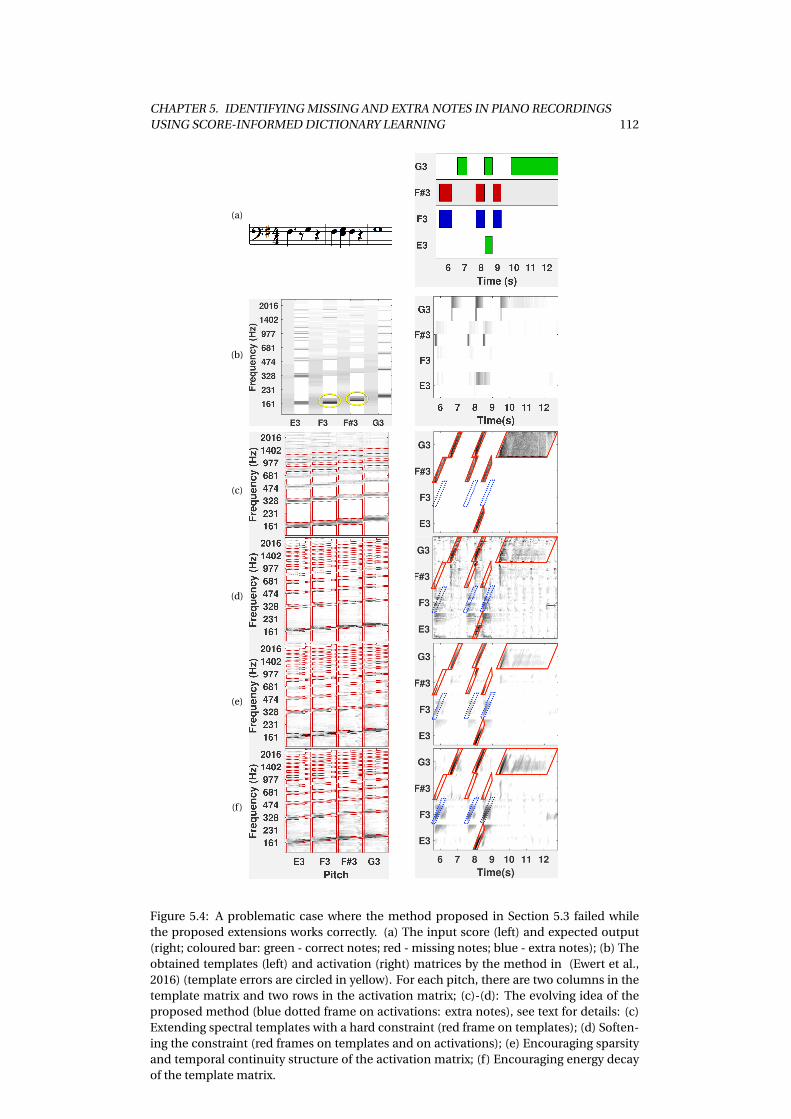
CHAPTER 5. IDENTIFYING MISSING AND EXTRA NOTES IN PIANO RECORDINGSUSING SCORE-INFORMED DICTIONARY LEARNING 112
(a)
(b)
(c)
(d)
(e)
(f)
Figure 5.4: A problematic case where the method proposed in Section 5.3 failed whilethe proposed extensions works correctly. (a) The input score (left) and expected output(right; coloured bar: green - correct notes; red - missing notes; blue - extra notes); (b) Theobtained templates (left) and activation (right) matrices by the method in (Ewert et al.,2016) (template errors are circled in yellow). For each pitch, there are two columns in thetemplate matrix and two rows in the activation matrix; (c)-(d): The evolving idea of theproposed method (blue dotted frame on activations: extra notes), see text for details: (c)Extending spectral templates with a hard constraint (red frame on templates); (d) Soften-ing the constraint (red frames on templates and on activations); (e) Encouraging sparsityand temporal continuity structure of the activation matrix; (f) Encouraging energy decayof the template matrix.

CHAPTER 5. IDENTIFYING MISSING AND EXTRA NOTES IN PIANO RECORDINGSUSING SCORE-INFORMED DICTIONARY LEARNING 113
5.4.2 From Spectral Templates to Time-Frequency Patterns
The signal model used in Section 5.3 is NMF-based. A unifying aspect of most NMF
and sparse coding methods is that time and frequency information are strictly separated.
Therefore the NMF-based method proposed in the last section can neither model that a
specific template for the sustain part follows an attack template after a certain amount of
time, nor that the energy in a note decays in a specific way (Cheng et al., 2015). To adapt
the model closer to the acoustic characteristics of piano, the first proposed extension ex-
pands the dictionary based on individual templates to a dictionary of time-frequency pat-
terns. In particular, instead of using L = 2 templates, L is now set to the average note length
in frames.2 For example, in Fig. 5.4(c)-(f), the pattern length is L = 29. With such a drastic
increase in the number of parameters, it is unclear whether the learning process will still
function correctly. However, the score provides strong guidance to the learning process in
the first place, which will be additionally supported by new regularisers defined below.
Similarly to the baseline method, different constraints are applied to the attack and
the sustain templates. The first two templates of the extended dictionary are used for
the attack, considering the attack part of a piano sound is much shorter than the sustain
part. Fig. 5.4(c) shows the zero-based constraints using red frames in P and in A (the blue
frames are only informational and indicate where the extra F3 notes are active). Note that
the temporal constraints in A now have a diagonal structure to account for the intended
spectro-temporal interpretation of each pattern: if the `-th template for a pitch is active
in frame n, the (`+1)-th template should be active in frame (n+1) (given that the note
is still active in frame (n+1)). The same cost function c(P, A) is used as in Section 5.3,
which includes a reconstruction error term d(V ||P, A) and a spectral continuity regulariser
c1(P ) on the attack templates. As can be seen from Fig. 5.4(c), the template matrix after
the dictionary learning step captures more details compared to the previously proposed
method (b). However, due to the hard constraints, there is no activation for the actually
played F3 notes. The F#3 notes that are on the score get activated with the result that the
F#3 templates learn to represent the pitch F3, as shown by the energy at the bottom of the
2Here we try to balance the ability of the model to capture complete notes and the computational complex-ity. Currently, for notes which are longer than L, their length cannot be correctly modelled. If L is set to a largervalue, the longer notes can be modelled with the cost of higher computational complexity. However, as this workfocuses on identifying the missing and extra notes, the note length is of low importance, therefore L is set to theaverage note length to improve the computational efficiency.

CHAPTER 5. IDENTIFYING MISSING AND EXTRA NOTES IN PIANO RECORDINGSUSING SCORE-INFORMED DICTIONARY LEARNING 114
first partial of F#3 in Fig. 5.4(c). So, while this new signal model has potential to represent
more detail, it does not resolve the above problem.
5.4.3 From Hard to Soft Constraint Regions
A main reason why the dictionary learning in Section 5.4.1 fails is that the templates
needed to represent the F3 cannot be activated due to the use of hard constraints (also
discussed in a source separation context by Driedger et al. (2013)). Therefore, this subsec-
tion proposes another extension to change the hard constraints used in Section 5.4.1 into
arbitrarily strong regularisers, which encourage zeros but allow for exceptions if neces-
sary. More precisely, instead of using hard zero-based constraints, this extension applies
terms encouraging sparsity (similar to (Virtanen, 2007)) to the score-specified constraint
regions:
c2(P ) := ∑m,k,`
Pm,k,` · (1−M Pm,k,`) (5.4)
c1(A) := ∑k,`,n
Ak,`,n · (1−M Ak,`,n) (5.5)
where M P∈{0,1}M×(K ·L) and M A∈{0,1}(K ·L)×N denote with ones the unconstrained areas
of P and A, respectively, shown by the red frames in Fig. 5.4(d). Further, this extension
additionally tapers the constraint region on P for each partial (note the gradually nar-
rowed shape of the red frames), which encourages harmonics to transition from being a
little more broadband at the beginning to completely harmonic at the end of the note. c2
and c1 are essentially (potentially strong) `1 regularisers that are selectively applied to the
zero-value regions encoded in M P and M A , respectively.
Using these soft constraints also allows the merging of the dictionary learning and ex-
trapolation procedures (steps 2 and 3): time-frequency patterns are learned during the
dictionary learning step for all pitches. Since the pitches not found in the score typically
also will not occur in the performance, it is necessary to apply additional constraints to
obtain correct results. The idea here is to couple the time-frequency pattern for a pitch
not used in the score with that for the closest pitch found in the score. This way, the pat-
tern for a non-score pitch is constrained to be a shifted version of that for a score pitch.
Technically, this is related to shift-invariant dictionary learning (Smaragdis et al., 2008)
and more precisely to transformation-invariant NMF (Eggert et al., 2004).

CHAPTER 5. IDENTIFYING MISSING AND EXTRA NOTES IN PIANO RECORDINGSUSING SCORE-INFORMED DICTIONARY LEARNING 115
As shown on the left of Fig. 5.4(d), due to these changes, templates for F#3 no longer
contain energy associated with the F3 (in P ) and are activated less overall (in A). However,
the whole activation matrix is not very structured and contains a lot of noise, rendering
onset detection quite difficult. Therefore, more regularisers are introduced next to en-
courage further structure in P and A.
5.4.4 Encouraging Temporal Continuity in A
As mentioned in Section 5.4.2, the temporal constraints in A have a diagonal structure
to account for the intended spectro-temporal interpretation of each pattern. To further
enhance diagonal structures and discourage vertical and horizontal structures as well as
unnecessary fluctuations between neighbouring entries, this subsection introduces the
following regulariser term, similar to (Ewert and Sandler, 2016) :
c2(A) = ∑k,`,n
(Ak,`+1,n+1 − Ak,`,n)2 (5.6)
It can be seen as an anisotropic variant of the the total variation regulariser used in image
processing (Chan et al., 2005) and is related to temporal smoothness terms as used in
(Virtanen, 2007).
Further, another regulariser on A is introduced to encourage sparseness across all en-
tries, in order to have fewer but stronger diagonals resulting from c2. Note that c1 is con-
fined to the constrained regions.
c3(A) = ∑k,`,n
Ak,`,n (5.7)
As shown in Fig. 5.4 (e), after learning, the activation matrix becomes cleaner compared
to (d) and we can see the diagonal structure of three played notes appearing for F3. Note
that these three notes are not on the score so they are not able to benefit from the temporal
constraints on A. In this case, the temporal continuity regulariser can help them obtain
the expected diagonal structure.
However, there is still energy at the F#3 pitch, which was not played. Another problem
is that, in the corresponding templates (shown on the left side of (e)), the energy does not
decay with time. For example, in the first partial of E3, F3 and F#3, the energy is higher
in the last several templates than in the earlier ones, which does not correspond with the
true temporal evolution of piano tones.

CHAPTER 5. IDENTIFYING MISSING AND EXTRA NOTES IN PIANO RECORDINGSUSING SCORE-INFORMED DICTIONARY LEARNING 116
5.4.5 Encouraging Energy Decay in the Template Matrix
The next regulariser imposes a decay structure onto the spectral templates associated with
the sustain phase:
c3(P ) =∑k
∑m
∑`∈B
f (Pm,k,`−Pm,k,`−1), (5.8)
where B ⊂ {1, . . . ,L} denotes the index set of the sustain templates of the time-frequency
pattern of one pitch. f (·) is a function encouraging a smooth decrease in energy while
penalising sudden energy increases in the time direction. It is chosen as,
f (x) = (γx −1)e(γx−1) (5.9)
with γ > 0 being a non-linear parameter, see also Fig. 5.5. Using the differentiable c3,
decreases in energy in the time direction are effectively not penalised, while increases are
strongly discouraged. As shown in Fig. 5.4, after learning, individual patterns in P show
energy decays in the time direction. With these more accurate patterns, the three played
F3 notes are finally active in the activation matrix, while the F#3 notes (not played) are
correctly no longer activated.
It should be noted that this regulariser is not intended to model all details of the de-
cay process found in piano sounds. In particular, different partials decay at different rates
and thus various decay patterns are possible. Further, the coupling between strings adds
another layer of complexity to the decay pattern of a piano note, resulting in beating and
other fluctuations in energy that overlay the overall energy decay (Cheng et al., 2016). In-
stead of modelling these details, the main purpose of this regulariser is to assist in the
identification of the main effect, i.e. a strong exponential energy decay. Moreover, be-
cause the use of the dictionary of time-frequency patterns, here the decay could be mod-
elled by the templates rather than the activations in contrast to (Cheng et al., 2016), which
is easier to be implemented together with other regularisers in this work.
5.4.6 Parameter Estimation
In order to obtain P and A, the parameter estimation step needs to minimise the following
cost function,
c(P, A) = d(V ||P, A)+ζ1c1 (A)+ζ2c2 (A)+ζ3c3 (A)+η1c1 (P )+η2c2 (P )+η3c3 (P ). (5.10)

CHAPTER 5. IDENTIFYING MISSING AND EXTRA NOTES IN PIANO RECORDINGSUSING SCORE-INFORMED DICTIONARY LEARNING 117
Figure 5.5: Plot of function f (x) = (γx −1)e(γx−1) for γ= 10.
A similar multiplicative updating strategy to (Virtanen, 2007) is applied to alternately up-
date P and A until convergence. The gradients of terms in the cost function with respect
to A are given by:
∇Ad(V ||P, A) = PT1−PT V
PA, (5.11)
∇Ac1 (A) = 1−MA , (5.12)
[∇Ac2 (A)]k,`,n = 4Ak,`,n −2Ak,`−1,n−1 −2Ak,`+1,n+1, (5.13)
∇Ac3 (A) = 1. (5.14)
The gradient of the cost function is written as the difference between element-wise posi-
tive terms and negative terms:
[∇Ac(P, A)]k,`,n = [∇Ac+(P, A)]k,`,n − [∇Ac−(P, A)]k,`,n , (5.15)
[∇Ac+(P, A)]k,`,n =∑m
Pm,k,`+ζ1 +4ζ2 Ak,`,n +ζ3, (5.16)
[∇Ac−(P, A)]k,`,n =∑m
Pm,k,`Vm,n
(PA)m,n+ζ1(MA)k,`,n +2ζ2(Ak,`−1,n−1 + Ak,`+1,n+1). (5.17)
The update rule for A is given by:
Ak,`,n ← Ak,`,n · [∇Ac−(P, A)]k,`,n
[∇Ac+(P, A)]k,`,n. (5.18)
Similarly, the gradient of the cost function with regard to P can be split as:
[∇P c+(P, A)]m,k,` =∑n
Ak,`,n +IA (`)4η1Pm,k,`+η2
+IB(`)η3γ2(Pm,k,`eγ(Pm,k,`−Pm,k,`−1)−1 +Pm,k,`eγ(Pm,k,`+1−Pm,k,`)−1
)(5.19)

CHAPTER 5. IDENTIFYING MISSING AND EXTRA NOTES IN PIANO RECORDINGSUSING SCORE-INFORMED DICTIONARY LEARNING 118
[∇P c−(P, A)]m,k,` =∑n
Ak,`,nVm,n
(PA)m,n+IA (`)2η1Pm+1,k,`+IA (`)2η1Pm−1,k,`+η2(MP )m,k,`
+IB(`)η3γ2(Pm,k,`−1eγ(Pm,k,`−Pm,k,`−1)−1 +Pm,k,`+1eγ(Pm,k,`+1−Pm,k,`)−1
)(5.20)
where IA and IB are the indicator functions for A and B, respectively. The update rule
for P is given by
Pm,k,`← Pm,k,` ·[∇P c−(P, A)]m,k,`
[∇P c+(P, A)]m,k,`.(5.21)
As mentioned in Section 5.4.3, each non-score pitch uses the shifted version of the tem-
plates for the closest score pitch. While this is not problematic for the update of A (by
actually creating a shifted copy), the update for P needs to be adapted as the shifted and
unshifted versions need to be coupled, i.e. have to be updated jointly. Fortunately, the gra-
dients given above for score and non-score pitches can easily be merged and thus be used
to create a joint update, see (Eggert et al., 2004) for details.
Once the activation matrix A is obtained, the same strategy as in Section 5.3 is used for
onset detection and note classification. The only difference is that, to get ˆAk,n for onset
detection, all activation values associated with pitch k in frame n are summed together,
i.e., ˆAk,n = ∑` Ak,`,n . It is because the activations resulting from the spectro-temporal
dictionary are more discriminative for the attack part compared to the baseline method
and it is useful to include the attack part in A as well.
5.5 Experiments
This section reports experiments conducted to investigate the influence of different ex-
tensions on the baseline method, as well as evaluate the performance of the method with
and without these extensions.
5.5.1 Dataset & Evaluation Measure
5.5.1.1 Dataset
Table 5.1 shows the dataset of seven pieces used for the evaluation, which are selected
from the Associated Board of the Royal Schools of Music 2011/12 syllabus for grades 1 and
2. The dataset is originally introduced by Benetos et al. (2012) and the pieces were played
on a Yamaha U3 Disklavier with intentional mistakes compared to the original score. In

CHAPTER 5. IDENTIFYING MISSING AND EXTRA NOTES IN PIANO RECORDINGSUSING SCORE-INFORMED DICTIONARY LEARNING 119
Table 5.1: Pieces for evaluation
ID Composer Title1 Josef Haydn Symphony No. 94: Andante (Hob I:94-02)2 James Hook Gavotta (Op. 81 No. 3)3 Pauline Hall Tarantella4 Felix Swinstead A Tender Flower5 Johann Krieger Sechs musicalische Partien: Bourrée6 Johannes Brahms The Sandman (WoO 31 No. 4)7 Tim Richards (arr.) Down by the Riverside
total, there are 1600 correctly played notes, 111 missing notes and 116 extra notes. For
each piece, there is one audio recording, one MIDI file of the original score, and three
MIDI files annotating the correctly played, missing and extra notes. These annotations
were reviewed and corrected manually by listening to the corresponding audio recordings
before the experiments described below. The corrected annotations are available online3.
5.5.1.2 Audio Input
The audio data has a sampling rate of 44100 samples per second. It was converted to a
spectrogram using a Hann window, with a window size of 4096 and 50% overlap. Using a
weighted sum, the spectrogram is converted to a log-frequency scale using a resolution of
36 bins per octave.
5.5.1.3 Evaluation Measure
To evaluate a method, four performance metrics are calculated, Precision, Recall, F-
Measure and Accuracy, as used in the MIREX evaluation campaign (Downie, 2008) – how-
ever, separately for each class of notes. To this end, the annotation MIDI files provide
for the correctly played and extra notes the onset positions in the performance. For
each missing note, the corresponding MIDI file provides an onset position indicating
where that note would have been expected in the performance. By comparing the on-
set positions obtained by a method and those annotated in the ground truth, the perfor-
mance metrics can be obtained separately for each class of notes. A temporal tolerance of
T2 =±0.2s is used to account for the local alignment difficulties caused by playing errors.
3https://code.soundsoftware.ac.uk/projects/score-informed-piano-transcription-dataset

CHAPTER 5. IDENTIFYING MISSING AND EXTRA NOTES IN PIANO RECORDINGSUSING SCORE-INFORMED DICTIONARY LEARNING 120
5.5.2 Influence of Individual Parameters
To indicate the influence of different terms in the cost function, six groups of experiments
are conducted for the six regularisers used in the proposed method. In each group, one
parameter is changed with all others fixed.
5.5.2.1 Soft Mask-Constraint Regulariser on Activation Matrix
The influence of the parameter ζ1 is illustrated in Fig. 5.6(a). The weight controls c1 which
corresponds to a soft mask-constraint on A. The best results are obtained for ζ1 = 10−3.5.
The average accuracy for all three note classes declines if the activity constraint becomes
too strong, i.e. if activity outside the expected positions is heavily penalised and thus extra
notes cannot be modelled anymore.
5.5.2.2 Diagonal Structure Regulariser on Activation Matrix
Fig. 5.6 (b) shows a plot of the average accuracy against different values for the weight
ζ2, which is associated with the diagonal structure regulariser c2. The average accuracy of
correctly played and missing notes only changes slightly for ζ2 ∈ [0,10−1]. On the contrary,
the average accuracy for extra notes grows considerably with ζ2, peaking at ζ2 = 10−1. The
overall best results are obtained for ζ2 = 10−1. These results seem to indicate that the score
information alone might not be enough to guide the learning process in such a way that a
physically correct diagonal structure occurs in the activations and that this regulariser is
indeed needed.
5.5.2.3 Sparsity Regulariser on Activation Matrix
The influence of parameter ζ3, which balances the sparsity regulariser on the activation
matrix, is shown in Fig. 5.6 (c). The overall best results are obtained for ζ3 = 0.1. While
the change of ζ3 only leads to small fluctuations in the accuracy of identifying missing
notes, it has a larger impact on identifying extra notes. A possible reason is that, when
ζ3 is too small, the activation matrix is too noisy for detecting extra notes and when ζ3 is
too large, the activations for extra notes are being heavily suppressed. In both cases, the
signal-to-noise ratio for extra notes is low.

CHAPTER 5. IDENTIFYING MISSING AND EXTRA NOTES IN PIANO RECORDINGSUSING SCORE-INFORMED DICTIONARY LEARNING 121
(a)
(b)
(c)
(d)
(e)
(f)
Figure 5.6: Average accuracy as a function of different parameters. (a) activation con-straint ζ1; (b) diagonal structure regulariser ζ2; (c) activation sparsity regulariser ζ3; (d)spectral continuity regulariser; (e) template constraint η2; (f ) decay regulariser η3

CHAPTER 5. IDENTIFYING MISSING AND EXTRA NOTES IN PIANO RECORDINGSUSING SCORE-INFORMED DICTIONARY LEARNING 122
5.5.2.4 Spectral Continuity Regulariser on Template Matrix
Fig. 5.6 (d) shows the influence of parameter η1, which controls the spectral continuity
regulariser on the template matrix. The change of η1 has little impact on identifying cor-
rect and missing notes, while the highest accuracy of identifying extra notes is obtained
for η1 = 10.
5.5.2.5 Soft Mask-Constraint Regulariser on Template Matrix
Fig. 5.6 (e) shows the average accuracy for different values of the parameter η2, i.e. the
weight balancing the importance of the term c2 which implements a soft mask-constraint
on P (see Section 5.4.3). The average accuracy of identifying extra and missing notes in-
creases with η2 and peaks at η2 = 1, while the average accuracy for correctly played notes
remains steady. If η2 is increased beyond this point, similar to the template constraint
term, the accuracy for all three note classes drops, especially for the extra and missing
note classes.
5.5.2.6 Decay Structure Regulariser on Template Matrix
The influence of the parameter η3, which balances the importance of the decay structure
regulariser c3, is illustrated in Fig. 5.6 (f). The average accuracy for the correctly played
note class remains relatively static after a short increase. The average accuracies for miss-
ing and extra notes show an upwards trend with η3 first, followed by a decrease for the
extra notes with η3 > 10−0.3 and a slight decrease for the missing notes with η3 > 100.7.
The overall best results are obtained for η3 = 10−0.3, which seems to represent a reason-
able trade-off between model capacity and learning stability.
5.5.2.7 Discussion
Overall, varying the parameters has the least influence on the class of correctly played
notes and the largest influence on the extra notes. This is not really surprising as the score
provides strong information about the correctly played notes and thus the regularisers
are not required to provide additional help. For unexpected events, such as extra notes,
however, the regularisers are of much higher importance.

CHAPTER 5. IDENTIFYING MISSING AND EXTRA NOTES IN PIANO RECORDINGSUSING SCORE-INFORMED DICTIONARY LEARNING 123
One surprising observation is that the influence of the mask-constraint c1 on A is not
more pronounced in the results, as it essentially carries much of the temporal informa-
tion provided by the score. Indeed, using a low value for ζ1 more noise was observed in A
and yet the results do not differ much. Several aspects are important to explain this be-
haviour. First, even with a low value for ζ1, the score information is still used to initialise
A – which already adds a strong bias for the final result (note that, from an optimisation
point of view, NMF is a bi-convex problem and as such the error surface contains vari-
ous local minima). A second important aspect is the adaptive thresholding, which is part
of the onset detection. While c1 incorporates the note information as a soft constraint,
the adaptive thresholding as described in Section 5.3 employs the same information in a
more binary form. In particular, the adaptive method takes the noise level in A into ac-
count when choosing a threshold. Therefore, the stability of our method with respect to ζ1
can partially be attributed to the quality of the adaptive thresholding and its noise insen-
sitivity. For more complex pieces beyond the beginner level (i.e. intermediate levels and
beyond), however, the noise level may have a stronger impact on the results – such sce-
narios, however, were not within the scope of this thesis. However, with additional data,
this might be an interesting direction for future investigation.
With six regularisers in total, the optimisation of the joint parameter space is not triv-
ial as parameters might influence each other. Even using only five different settings for
each parameter leads to 56 = 15625 different configurations in a grid search. To test each
configuration on all the pieces will take around 50 seconds, which will be summed up
to 9 days. However, assuming that most dependencies are already observable in pairs of
parameters (i.e. in contrast to dependencies that only occur comparing two groups of
parameters jointly), the search space can be decreased drastically. In particular, with six
parameters there are only(6
2
)= 15 different combinations. Testing five different values per
parameter leads to 25 configurations to be tested for each combination and thus to a to-
tal of 375 configurations and corresponding evaluations on the whole dataset, which will
take around 5 hours.
Overall, interaction effects were not found between most parameters, which justifies
optimising them individually. However, a somewhat complex interaction was shown be-
tween the template mask-constraint parameter η2 and the diagonal structure parameter

CHAPTER 5. IDENTIFYING MISSING AND EXTRA NOTES IN PIANO RECORDINGSUSING SCORE-INFORMED DICTIONARY LEARNING 124
Figure 5.7: Interaction between parameters ζ2 and η2 as they influence identification ac-curacy for all three types of notes.
ζ2. Fig. 5.7 shows various plots illustrating the performance of the proposed method for
several combinations of the two parameters – plotted separately for the three note classes.
If there would be no interaction, the plots would not cross. However, the interaction is ob-
served in particular for higher values of η2. For example, for extra notes, when the value of
η2 is high, the accuracy improves with higher values of ζ2. When the value of η2 is low, the
opposite happens. While this interaction might just be a property of our dataset and its
size, it might also be explained by the fact that a strong η2 leads to stronger constraints on
P , which might not always be appropriate. A stronger value for ζ2 might make sure in this
case that “unexplained" residual energy (resulting from enforcing incorrect constraints) is
suppressed in A by other means and thus does not lead to wrong detections.
5.5.3 Comparison Between the Baseline Method and Extended Method
This subsection compares the performance of the baseline method with the extended
method. The parameters for the extensions are set to a configuration found to perform

CHAPTER 5. IDENTIFYING MISSING AND EXTRA NOTES IN PIANO RECORDINGSUSING SCORE-INFORMED DICTIONARY LEARNING 125
Table 5.2: Average Evaluation Results of three Methods for Correctly Played Notes(C), ExtraNotes (E) and Missing Notes (M)
Method Class Prec. Recall F-Meas. Accur.
ExtendedC 0.996 0.989 0.992 0.984E 0.876 0.840 0.849 0.752M 0.895 0.980 0.932 0.869
BaselineC 0.994 0.991 0.993 0.986E 0.814 0.750 0.770 0.640M 0.928 0.970 0.945 0.899
Benetos et al. (2012)C - - - 0.932E - - - 0.605M - - - 0.492
well as described above: ζ1 = 10−3.5,ζ2 = 0.1,ζ3 = 0.1,η1 = 10,η2 = 1,η3 = 0.5.
The average evaluation results of all seven pieces are shown in Table 5.2. In particular,
the reported F-measure is an average over the individual F-measure values, rather than
computed from the average precision and recall given in Table 5.2. Table 5.2 also includes
the average accuracy of the method proposed by Benetos et al. (2012) as a reference, how-
ever, note that the evaluation for other two proposed methods uses a slightly modified
ground truth as mentioned in 5.5.1.
For the correctly played notes (C), the extended method and baseline method have
similar performances on all four evaluation measures. The extended method outperforms
the baseline method for the extra note class (E), on all the measures. For example, the av-
erage accuracy improves by 17%, from 0.640 to 0.752. As for the missing note class (M),
the extended method is slightly worse (by 2%) than the baseline method but still at a sim-
ilar level, comparing 0.869 with 0.899. Note that the amounts of missing notes and extras
notes are similar (see Section 5.5.1).
5.6 Conclusion
This chapter extended a score-informed transcription method to identify missing and
extra notes in piano recordings. By incorporating score information into the dictio-
nary learning process, the baseline method yields spectral patterns for each pitch closely
adapted to the given recording. To better account for the specific characteristics of pi-
ano sounds and local deviations of the performance from the score, this chapter intro-
duced several extensions to the baseline method. As demonstrated by experiments with a

CHAPTER 5. IDENTIFYING MISSING AND EXTRA NOTES IN PIANO RECORDINGSUSING SCORE-INFORMED DICTIONARY LEARNING 126
dataset of pieces for piano beginners, the extensions improve the accuracy in identifying
extra notes over the baseline method.
One issue that could be addressed in future work is the lack of data. Informally, experi-
ments showed that the proposed method performed differently depending on the amount
and the type of deviation the performance has from the given score. It would be interest-
ing to create a new dataset to test the proposed method across a variety of scenarios. For
example, in performance analysis, the number of playing mistakes can be expected to
be less compared to a music tutoring application, while deviations due to musical inter-
pretation might increase. Further, since the alignment method in use was not designed
to deal with local changes in the order of notes, such as broken or arpeggiated chords,
the score constraints might provide incorrect information to the transcription process in
such scenarios. Similarly, in the music tutoring application, an extremely large number of
errors might occur in some cases, which might lead to the alignment getting lost and thus
corrupting the transcription result. Therefore, future work could investigate strategies to
adapt the score information better to different application scenarios.
Another issue for future work is the computational complexity. Since the dictionary
is extended to L templates for each pitch (compared to two templates in the baseline
method), the computational cost for the dictionary learning step is L/2 times higher. For
example, for an recording of around 1 min in the experiment dataset, the computing time
of the proposed method is around 1 min, comparing to 7 seconds of the baseline method.
For a music tutoring system, there might be constraints on the run-time and thus it will be
beneficial to investigate strategies to lower the computational cost without affecting the
overall accuracy of the system.

CH
AP
TE
R
6CONCLUSION
This thesis proposed several novel computational methods in the context of music align-
ment and score-informed transcription. Two music alignment methods were presented in
Chapters 3 and 4, focusing on improving the robustness against local differences between
the versions to be aligned. Chapter 5 presented a score-informed transcription method
that applies score to performance alignment to exploit score information in the learning
process of a dictionary-based transcription method. In the following, Section 6.1 sum-
marises the main achievements of this thesis and Section 6.2 discusses some possible fu-
ture directions.
6.1 Summary of Contributions
Despite the fact that the accuracy of music alignment methods has improved consider-
ably in the last decade, the task of music alignment remains challenging, such as in the
cases where there are substantial local differences between versions. This thesis proposed
methods aiming to improve the alignment robustness for two scenarios. By applying an
accurate and robust alignment method, this thesis also presented a score-informed tran-
scription method.
127

CHAPTER 6. CONCLUSION 128
Most state-of-the-art methods employ pairwise alignment approaches and yield high
accuracy in many cases. However, they may fail when strong local differences occur be-
tween two versions. In contrast, the work presented in Chapter 3 exploits the fact that
there are often multiple versions of the piece of music available, and aligning them jointly
can stabilise the system with additional information of how one section might be inter-
preted or which acoustic conditions may arise. Two such joint alignment methods were
proposed, Progressive Alignment and Profile HMM. They were both inspired by the multi-
ple sequence alignment task in bio-informatics, but specifically adapted to take the char-
acteristics of music signals into account. Experiments with 376 recordings from 9 clas-
sical piano pieces showed that the two proposed methods not only decrease the overall
standard deviation of the alignment error, but also improve the average alignment accu-
racy. These results indicate that the proposed methods are particularly useful to effec-
tively reduce large alignment errors, i.e. to increase the overall alignment robustness. The
two proposed methods are conceptually different but share some algorithmic similari-
ties. Systematic experiments were performed to further understand their behaviour. They
showed that while both methods can improve the alignment robustness if a large num-
ber of versions are available, Progressive Alignment outperforms state-of-the-art pairwise
alignment methods even with a small set of versions (three or more).
Chapter 4 focused on improving alignment robustness in the presence of a particular
musical parameter: asychronies between musical voices. Most current alignment meth-
ods have made the simplifying assumption that simultaneous notes in the score are also
played concurrently in a performance. Musicians, however, sometimes incorporate asyn-
chronies between voices for expressive reasons. In such cases, the alignment accuracy of
current methods may drop measurably on a local level. To handle such asychronies be-
tween the melody and the accompaniment, Chapter 4 presented a novel method which
firstly separates a score into two voices, then jointly aligns them and the audio stream
with a three-dimensional Dynamic Time Warping algorithm. To avoid a loss of accuracy
caused by splitting the score information into two separate voices and to lower the com-
putational costs, two constraints were introduced in computing the three dimensional
cost matrix. The first one limits the amount of allowed asynchrony based on the fact that
the asynchronies in practice are not arbitrarily high. The second constraint is based on a

CHAPTER 6. CONCLUSION 129
projection of an alignment path obtained by a standard two dimensional method to the
three dimensional cost matrix. This way, the alignment path is forced to run close to the
projected path, providing improved robustness and a reduced computational complex-
ity. Experiments with three piano pieces by Chopin (with relatively strong asynchronies)
and three pieces from Bach’s Well-Tempered Clavier (with little asynchrony) showed that
the proposed method improves the alignment accuracy for the pieces with strong asyn-
chronies and preserves the alignment accuracy for those without.
By establishing links between different representations of the same piece of music,
alignment techniques enable various applications. One of them is to improve the accu-
racy of automatic music transcription by exploiting the score as prior knowledge, available
in certain scenarios such as music tutoring. After aligning the score to the given audio
recording, the idea is to build a score-informed dictionary learning process, yielding for
each pitch a spectral pattern closely adapted to the given recording. This way, a tran-
scription method is tailored to identify the missing and extra notes from the given audio
recording compared to the score. Chapter 5 presented such a score-informed transcrip-
tion system which extends the state-of-the-art approach (Ewert et al., 2016) to better ac-
count for the properties of piano sounds and the possible deviations of the performance
from the score. Experiments with a dataset of pieces for piano beginners showed that the
proposed method considerably improves the accuracy in identifying extra notes.
6.2 Future Directions
This section suggests several possible directions to extend or apply the work described in
this thesis.
Handling structural differences in joint alignment methods
The work presented in this thesis has not dealt with alignment in the case of structural dif-
ferences between performances. However, preliminary experiments have been performed
using the Progressive Alignment method proposed in Chapter 3 to align a set of perfor-
mances, including recordings with structural differences compared to the others. Despite
such structural differences, the method correctly aligned corresponding positions. If the
previously aligned template contains a certain section that the new performance to be

CHAPTER 6. CONCLUSION 130
aligned skips, the method inserts the corresponding gap symbols when the performance
is incorporated into the template. If the new performance contains an inserted section,
then the method opens the corresponding gaps in the template. However, if the inserted
section is a repeat, the method is currently unable to identify the section as such and thus
cannot align the repeated section correctly. To do so, a suitable repetitive structure extrac-
tion method could be applied; see (Paulus et al., 2010) for an overview.
Annotation transfer with joint alignment of multiple performances
The joint alignment methods proposed in Chapter 3 can be applied to transfer annota-
tions created for one performance to other versions. For instance, if one performance is
annotated with beat positions, the joint alignment method can be used to map the an-
notations to other performances of the same piece, instead of aligning all versions to the
annotated version using pairwise alignment. Aligning multiple versions simultaneously
by the joint alignment method can avoid the inconsistencies between different pairwise
alignments.
Handling asynchrony between different instruments
The work presented in Chapter 4 is concerned with the asynchrony between voices in
piano performances. This idea, however, can be extended to deal with scenarios with
asynchronies between instruments, such as in music ensembles, or asynchronies between
the human voice and the accompaniment in a karaoke setting.
Improving the score MIDI to performance MIDI alignment tool
To create the ground truth for experiments in Chapter 4, a graphical user interface was
developed in Matlab for manually correcting results of an automatic alignment between
a score and a performance MIDI file. It can read a score in MusicXML or MIDI format. If a
MusicXML version is available, the tool converts it to MIDI to perform the alignment, and
exploits the coordination information contained in the MusicXML to link each score note
to its corresponding score image location. This way, the tool can provide the appropriate
score excerpt as a reference for manual correction of the alignment.

CHAPTER 6. CONCLUSION 131
Currently, the tool has several weaknesses that could be addressed. Firstly, the auto-
matic alignment based on a simple LCS method could be improved. The method could be
replaced by a more sophisticated approach to reduce the amount of manual work needed.
Secondly, the tool could be implemented in a more suitable programming language rather
than Matlab. When dealing with long pieces of music, the current Matlab-based interface
has a slow response time.
Score-informed transcription of other instruments
The score-informed transcription system in Chapter 5 is specifically for piano recordings.
The idea, however, can be extended to other instruments, while taking their specific char-
acteristics into account. For example, for transcribing string instruments, variability in the
fundamental frequency could be captured by shift-invariant dictionary learning. With the
score as prior information, it is possible to learn instrument-specific dictionaries because
the expected time and pitch of instrumental activity is available for each instrument.
Score-informed performance analysis
The score-informed transcription system has the potential to be a basis for various per-
formance analysis tasks, as deviations of the performance from the score can be detected.
For the music tutoring application described in Chapter 5, the expected deviation is lim-
ited to missing and extra notes. However, in the case of more advanced performances,
deviations might be the result of deliberate playing techniques. Such scenarios would re-
quire a more fine-grained note-level alignment.
6.3 Closing Remarks
Music alignment, one of the fundamental steps of digital music analysis, modelling and
processing, has been actively researched in the last decades. Various methods have been
proposed and the state-of-the-art performance has already achieved high accuracy in
many cases. However, the robustness of current alignment methods may be challenged by
the variation of music expression and acoustic conditions. The work of this thesis made
efforts to improve robustness in two specific scenarios. The author hopes this thesis will

CHAPTER 6. CONCLUSION 132
inspires further research in the direction of building alignment methods that are robust to
a wide range of scenarios.
An accurate and robust alignment can establish links between different versions of
music, so as to enhance the experience of people interacting with music in real life appli-
cations. For example, Arzt et al. (2015) used automatic score following in a live concert,
where multiple performances were aligned to the score in parallel to provide additional in-
formation to improve the alignment robustness (a similar idea as Chapter 3). Music align-
ment can also assist performance analysis; for example, manual score to performance
alignment has been used in an online course about Haydn’s Op.20 No.5 string quartet1.
Meanwhile, there are quite a few commercial applications employ music alignment al-
gorithms for concert enhancement2 and piano learning assistance3,4. For piano learning
assistance apps3,4, the current use of music alignment is to provide score following func-
tionality for practice and performance analysis based on comparison with expert pianists.
For evaluating the student’s performance in the aspect of reproducing the score faithfully,
the piano learning assistance app (melomemo)4 requires wearable sensors or a camera to
capture the playing mistakes. The author believes the idea explored in Chapter 5, which
employs music alignment to build a score-informed transcription system for identifying
missing and extra notes from audio recordings has potential to benefit such music tutor-
ing applications. However, the work in this thesis is just an early step; the author hopes
it will inspire further research toward a mature system for identifying performance devia-
tions from the score.
1https://lagunita.stanford.edu/courses/course-v1:HumanitiesSciences+StringQuartet1+selfpaced/info
2https://www.philorch.org/concert/livenote#3http://tido-music.com/4http://www.raintai.com/index.html

REFERENCES
J. Abeßer, K. Frieler, E. Cano, M. Pfleiderer, and W.-G. Zaddach. Score-Informed Analysis
of Tuning, Intonation, Pitch Modulation, and Dynamics in Jazz Solos. IEEE/ACM Trans-
actions on Audio, Speech, and Language Processing, 25(1):168–177, 2017.
A. Arzt and G. Widmer. Real-time Music Tracking using Multiple Performances as a Ref-
erence. In Proceedings of the 16th International Society for Music Information Retrieval
Conference (ISMIR), pages 357–363, Málaga, Spain, 2015.
A. Arzt, G. Widmer, and S. Dixon. Automatic Page Turning for Musicians via Real-Time
Machine Listening. In Proceedings of the European Conference on Artificial Intelligence
(ECAI), pages 241–245, Patras, Greece, 2008.
A. Arzt, S. Böck, S. Flossmann, H. Frostel, M. Gasser, and G. Widmer. The Complete Clas-
sical Music Companion v0.9. In Proceedings of the AES International Conference on Se-
mantic Audio, pages 133–137, London, UK, 18–20 2014.
A. Arzt, H. Frostel, T. Gadermaier, M. Gasser, M. Grachten, and G. Widmer. Artificial Intel-
ligence in the Concertgebouw. In Proceedings of the 24th International Joint Conference
on Artificial Intelligence (IJCAI), pages 2424–2430, 2015.
D. Basaran, A. T. Cemgil, and E. AnarÎzm. A Probabilistic Model-Based Approach for Align-
ing Multiple Audio Sequences. IEEE/ACM Transactions on Audio, Speech and Language
Processing, 23(7):1160–1171, 2015.
M. A. Bartsch and G. H. Wakefield. To Catch a Chorus: Using Chroma-based Representa-
tions for Audio Thumbnailing. In Proceedings of the IEEE Workshop on Applications of
Signal Processing to Audio and Acoustics (WASPAA), pages 15–18, New Paltz, NY, USA,
2001.
133

M. A. Bartsch and G. H. Wakefield. Audio Thumbnailing of Popular Music Using Chroma-
based Representations. IEEE Transactions on Multimedia, 7(1):96–104, 2005.
J. P. Bello and J. Pickens. A Robust Mid-level Representation for Harmonic Content in
Music Signals. In Proceedings of the 6th International Conference on Music Information
Retrieval (ISMIR), pages 304–311, London, UK, 2005.
J. P. Bello Correa. Towards the Automated Analysis of Simple Polyphonic Music: A
Knowledge-based Approach. PhD thesis, University of London, 2003.
E. Benetos and S. Dixon. A Shift-Invariant Latent Variable Model for Automatic Music
Transcription. Computer Music Journal, 36(4):81–94, 2012.
E. Benetos and S. Dixon. Multiple-Instrument Polyphonic Music Transcription using
a Temporally Constrained Shift-Invariant Model. Journal of the Acoustical Society of
America, 133(3):1727–1741, 2013.
E. Benetos, A. Klapuri, and S. Dixon. Score-Informed Transcription for Automatic Piano
Tutoring. In Proceedings of the 20th European Signal Processing Conference (EUSIPCO),
pages 2153–2157, Bucharest, Romania, 2012.
E. Benetos, S. Dixon, D. Giannoulis, H. Kirchhoff, and A. Klapuri. Automatic Music Tran-
scription: Challenges and Future Directions. Journal of Intelligent Information Systems,
41(3):407–434, 2013.
S. Bengio. An Asynchronous Hidden Markov Model for Audio-Visual Speech Recognition.
In Advances in Neural Information Processing Systems 15 (NIPS), pages 1213–1220, Mon-
tréal, Canada, 2002.
M. G. Bergomi. Dynamical and Topological Tools for (Modern) Music Analysis. PhD thesis,
Université Pierre et Marie Curie (Paris 6), 2015.
N. Bertin, R. Badeau, and E. Vincent. Enforcing Harmonicity and Smoothness in Bayesian
Non-negative Matrix Factorization Applied to Polyphonic Music Transcription. IEEE
Transactions on Audio, Speech, and Language Processing, 18(3):538–549, 2010.
134

S. Böck and M. Schedl. Polyphonic Piano Note Transcription with Recurrent Neural Net-
works. In Proceedings of the IEEE International Conference on Acoustics, Speech and
Signal Processing (ICASSP), pages 121–124, Kyoto, Japan, 2012.
M. A. Casey, R. Veltkamp, M. Goto, M. Leman, C. Rhodes, and M. Slaney. Content-based
Music Information Retrieval: Current Directions and Future Challenges. Proceedings of
the IEEE, 96(4):668–696, 2008.
W. Chai. Semantic Segmentation and Summarization of Music: Methods Based on Tonal-
ity and Recurrent Structure. IEEE Signal Processing Magazine, 23(2):124–132, 2006.
T. Chan, S. Esedoglu, F. Park, and A. Yip. Recent Developments in Total Variation Image
Restoration. Mathematical Models of Computer Vision, 17, 2005.
T.-S. Chan, T.-C. Yeh, Z.-C. Fan, H.-W. Chen, L. Su, Y.-H. Yang, and R. Jang. Vocal Activity
Informed Singing Voice Separation with the iKala Dataset. In Proceedings of the IEEE In-
ternational Conference on Acoustics, Speech and Signal Processing (ICASSP), pages 718–
722, Brisbane, Australia, 2015.
N. P. Chapman and J. Chapman. Digital Multimedia. John Wiley & Sons, Inc., 2000.
C.-T. Chen, J.-S. R. Jang, and W. Liou. Improved Score-Performance Alignment Algorithms
on Polyphonic Music. In Proceedings of the IEEE International Conference on Acoustics,
Speech and Signal Processing (ICASSP), pages 1365–1369, Florence, Italy, 2014. IEEE.
T. Cheng, S. Dixon, and M. Mauch. Modelling the Decay of Piano Sounds. In Proceedings of
the IEEE International Conference on Acoustics, Speech, and Signal Processing (ICASSP),
pages 594–598, Brisbane, Australia, 2015.
T. Cheng, M. Mauch, E. Benetos, and S. Dixon. An Attack/Decay Model for Piano Tran-
scription. In Proceedings of the 17th International Society for Music Information Re-
trieval Conference (ISMIR), New York City, NY, USA, 2016.
E. Chew and X. Wu. Separating Voices in Polyphonic Music: A Contig Mapping Approach.
In Computer Music Modelling and Retrieval (CMMR), pages 1–20, Pisa, Italy, 2005.
135

T. Cho, R. J. Weiss, and J. P. Bello. Exploring Common Variations in State of the Art Chord
Recognition Systems. In Proceedings of the Sound and Music Computing Conference
(SMC), pages 1–8, Barcelona, Spain, 2010.
M. G. Christensen and A. Jakobsson. Multi-Pitch Estimation. Synthesis Lectures on Speech
and Audio Processing, Morgan and Claypool Publishers, 2009.
E. Clarke. Expression in Performance: Generativity, Perception and serniosis. In J. Rink,
editor, The Practice of Performance: Studies in Musical Interpretation, pages 21–54.
Cambridge University Press, Cambridge, UK, 1995.
A. Cont. Realtime Audio to Score Alignment for Polyphonic Music Instruments using
Sparse Non-Negative Constraints and Hierarchical HMMs. In Proceedings of the IEEE
International Conference on Acoustics, Speech and Signal Processing (ICASSP), volume 5,
Toulouse, France, 2006.
A. Cont. A Coupled Duration-Focused Architecture for Real-Time Music-to-Score Align-
ment. IEEE Transactions on Pattern Analysis and Machine Intelligence, 32(6):974–987,
2010.
A. Cont, D. Schwarz, and N. Schnell. Training IRCAM’s Score Follower. In Proceedings of
the IEEE International Conference on Acoustics, Speech and Signal Processing (ICASSP),
Philadelphia,PA, USA, 2005.
N. Cook. Beyond the Score: Music as Performance. Oxford University Press, 2014.
S. J. Cox. Hidden Markov Models for Automatic Speech Recognition: Theory and Applica-
tion. In C. Wheddon and R. Linggard, editors, Speech and Language Processing, pages
209–230. Chapman & Hall, London, UK, 1990.
R. B. Dannenberg. An On-Line Algorithm for Real-Time Accompaniment. In Proceedings
of the International Computer Music Conference (ICMC), pages 193–198, Paris, France,
1984.
R. B. Dannenberg and M. Goto. Music Structure Analysis from Acoustic Signals. In
D. Havelock, S. Kuwano, and M. Vorländer, editors, Handbook of Signal Processing in
Acoustics, volume 1, pages 305–331. Springer, New York City, NY, USA, 2008.
136

R. B. Dannenberg and N. Hu. Polyphonic audio matching for score following and intel-
ligent audio editors. In Proceedings of the International Computer Music Conference
(ICMC), pages 27–34, San Francisco, USA, 2003.
R. B. Dannenberg and C. Raphael. Music Score Alignment and Computer Accompani-
ment. Communications of the ACM, Special Issue: Music Information Retrieval, 49(8):
38–43, 2006.
R. B. Dannenberg, M. Sanchez, A. Joseph, P. Capell, R. Joseph, and R. Saul. A Computer-
based Multi-media Tutor for Beginning piano Students. Journal of New Music Research,
19(2-3):155–173, 1990.
C. Dittmar, E. Cano, J. Abeßer, and S. Grollmisch. Music Information Retrieval Meets Music
Education. In Multimodal Music Processing, volume 3 of Dagstuhl Follow-Ups, pages
95–120. Schloss Dagstuhl–Leibniz-Zentrum für Informatik, 2012.
S. Dixon and G. Widmer. MATCH: A Music Alignment Tool Chest. In Proceedings of the
6th International Conference on Music Information Retrieval (ISMIR), pages 492–497,
London, UK, 2005.
M. Dorfer, A. Arzt, and G. Widmer. Towards Score Following in Sheet Music Images. In
In Proceedings of 17th International Society for Music Information Retrieval Conference
(ISMIR), New York City, NY, USA, 2016a.
M. Dorfer, A. Arzt, and G. Widmer. Towards End-to-End Audio-Sheet-Music Retrieval. In
NIPS 2016 End-to-end Learning for Speech and Audio Processing Workshop, Barcelona,
Spain, 2016b.
J. S. Downie. The Music Information Retrieval Evaluation eXchange (2005–2007): A Win-
dow into Music Information Retrieval Research. Acoustical Science and Technology, 29
(4):247–255, 2008.
J. Driedger, H. Grohganz, T. Prätzlich, S. Ewert, and M. Müller. Score-Informed Audio
Decomposition and Applications. In Proceedings of the ACM International Conference
on Multimedia (ACM-MM), pages 541–544, Barcelona, Spain, 2013.
137

Z. Duan and B. Pardo. A State Space Model for Online Polyphonic Audio-Score Alignment.
In Proceedings of the IEEE International Conference on Acoustics, Speech, and Signal Pro-
cessing (ICASSP), pages 197–200, Prague, Czech Republic, 2011.
R. Durbin, S. R. Eddy, A. Krogh, and G. Mitchison. Biological Sequence Analysis : Prob-
abilistic Models of Proteins and Nucleic Acids. Cambridge University Press, New York,
USA, 1999.
A. Earis. An Algorithm to Extract Expressive Timing and Dynamics from Piano Recordings.
Musicae Scientiae, 11(2):155–82, 2007.
J. Eggert, H. Wersing, and E. Korner. Transformation-Invariant Representation and NMF.
In Proceedings of the 2004 IEEE International Joint Conference on Neural Networks,
pages 2535–2539, Budapest, Hungary, 2004.
V. Emiya, R. Badeau, and B. David. Multipitch Estimation of Piano Sounds using a New
Probabilistic Spectral Smoothness Principle. IEEE Transactions on Audio, Speech and
Language Processing, 18(6):1643–1654, 2010.
S. Ewert and M. Müller. Estimating Note Intensities In Music Recordings. In Proceedings of
the IEEE International Conference on Acoustics, Speech, and Signal Processing (ICASSP),
pages 385–388, Prague, Czech Republic, 2011.
S. Ewert and M. Sandler. Piano Transcription in the Studio Using an Extensible Alternat-
ing Directions Framework. IEEE/ACM Transactions on Audio, Speech, and Language
Processing, 24(11):1983–1997, 2016.
S. Ewert, M. Müller, and R. B. Dannenberg. Towards Reliable Partial Music Alignments Us-
ing Multiple Synchronization Strategies. In Proceedings of the International Workshop
on Adaptive Multimedia Retrieval (AMR), Lecture Notes in Computer Science (LNCS),
volume 6535, pages 35–48, Madrid, Spain, 2009a.
S. Ewert, M. Müller, and P. Grosche. High Resolution Audio Synchronization Using Chroma
Onset Features. In Proceedings of the IEEE International Conference on Acoustics,
Speech, and Signal Processing (ICASSP), pages 1869–1872, Taipei, Taiwan, 2009b.
138
S. Ewert, B. Pardo, M. Müller, and M. D. Plumbley. Score-Informed Source Separation for
Musical Audio Recordings: An Overview. IEEE Signal Processing Magazine, 31(3):116–
124, 2014.
S. Ewert, M. D. Plumbley, and M. Sandler. A Dynamic Programming Variant of Non-
Negative Matrix Deconvolution for the Transcription of Struck String Instruments. In
Proceedings of the IEEE International Conference on Acoustics, Speech, and Signal Pro-
cessing (ICASSP), pages 569–573, Brisbane, Australia, 2015.
S. Ewert, S. Wang, M. Müller, and M. Sandler. Score-Informed Identification of Missing
and Extra Notes in Piano Recordings. In Proceedings of the 17th International Society for
Music Information Retrieval Conference (ISMIR), pages 30–36, New York City, NY, USA,
2016.
D. Fabian, R. Timmers, and E. Schubert. Expressiveness in Music Performance: Empirical
Approaches across Styles and Cultures. Oxford University Press, USA, 2014.
C. Fremerey, M. Müller, and M. Clausen. Handling Repeats and Jumps in Score-
Performance Synchronization. In Proceedings of the 11th International Conference on
Music Information Retrieval (ISMIR), pages 243–248, Utrecht, The Netherlands, 2010.
T. Fujishima. Realtime Chord Recognition of Musical Sound: A System Using Common
Lisp Music. In Proceedings of the International Computer Music Conference (ICMC),
pages 464–467, Beijing, China, 1999.
A. Gabrielsson. Music Performance Research at the Millennium. Psychology of Music, 31
(3):221–272, 2003.
W. Goebl. Numerisch-klassifikatorische Interpretationsanalyse mit dem ‘Bösendorfer
Computerflügel’. Master’s thesis, Universität Wien, 1999a.
W. Goebl. The Vienna 4x22 Piano Corpus. http://dx.doi.org/10.21939/4X22, 1999b.
W. Goebl. Skilled Piano Performance: Melody Lead Caused by Dynamic Differentiation.
In Proceedings of the 6th International Conference on Music Perception and Cognition,
Keele, UK, 2000.
139

W. Goebl. Melody Lead in Piano Performance: Expressive Device or Artifact? The Journal
of the Acoustical Society of America, 110:563–572, 2001.
W. Goebl, S. Dixon, G. De Poli, A. Friberg, R. Bresin, and G. Widmer. Sense in Expressive
Music Performance: Data Acquisition, Computational Studies, and Models. In P. Polotti
and D. Rocchesso, editors, Sound to Sense-Sense to Sound: A State of the Art in Sound
and Music Computing, pages 195–242. Logos Verlag Berlin, 2008.
E. Gómez. Tonal Description of Polyphonic Audio for Music Content Processing. IN-
FORMS Journal on Computing, 18(3):294–304, 2006.
M. Grachten, M. Gasser, A. Arzt, and G. Widmer. Automatic Alignment of Music Perfor-
mances with Structural Differences. In Proceedings of 14th International Society for
Music Information Retrieval Conference (ISMIR), Curitiba, Brazil, 2013.
L. Grubb and R. B. Dannenberg. A Stochastic Method of Tracking a Vocal Performer. In
Proceedings of the International Computer Music Conference (ICMC), pages 301–308,
Ann Arbor, MI, USA, 1997.
D. Gusfield. Algorithms on Strings, Trees, and Sequences: Computer Science and Computa-
tional Biology. Cambridge University Press, New York, NY, USA, 1997.
P. E. Hart, N. J. Nilsson, and B. Raphael. A Formal Basis for the Heuristic Determination
of Minimum Cost Paths. IEEE Transactions on Systems Science and Cybernetics, 4(2):
100–107, 1968.
C. Harte and M. Sandler. Automatic Chord Identification Using a Quantised Chromagram.
In Proceedings of the 118th AES Convention, Barcelona, Spain, 2005.
H. Heijink, P. Desain, H. Honing, and L. Windsor. Make Me a Match: An Evaluation of
Different Approaches to Score-Performance Matching. Computer Music Journal, 24(1):
43–56, 2000.
G. Holt, M. Reinders, and E. Hendriks. Multi-Dimensional Dynamic Time Warping for
Gesture Recognition. In Advanced School for Computing and Imaging, Delft, The
Netherlands, 2007.
140

R. Howat. What Do We Perform? In J. Rink, editor, The Practice of Performance: Studies in
Musical Interpretation, pages 3–20. Cambridge University Press, Cambridge, UK, 1995.
N. Hu, R. B. Dannenberg, and G. Tzanetakis. Polyphonic Audio Matching and Alignment
for Music Retrieval. In Proceedings of the IEEE Workshop on Applications of Signal Pro-
cessing to Audio and Acoustics (WASPAA), New Paltz, NY, USA, 2003.
F. Itakura. Minimum Prediction Residual Principle Applied to Speech Recognition. IEEE
Transactions on Acoustics, Speech, and Signal Processing, 23(1):67–72, 1975.
K. Itoyama, M. Goto, K. Komatani, T. Ogata, and H. G. Okuno. Instrument Equalizer For
Query-By-Example Retrieval: Improving Sound Source Separation Based On Integrated
Harmonic And Inharmonic Models. In Proceedings of the 9th International Conference
for Music Information Retrieval (ISMIR), pages 133–138, Philadelphia, PA, USA, 2008.
C. Joder, S. Essid, and G. Richard. A Comparative Study of Tonal Acoustic Features for
a Symbolic Level Music-to-Score Alignment. In Proceedings of the IEEE International
Conference on Acoustics, Speech, and Signal Processing (ICASSP), Dallas, TX, USA, 2010.
C. Joder, S. Essid, and G. Richard. A Conditional Random Field Framework for Robust and
Scalable Audio-to-Score Matching. IEEE Transactions on Audio, Speech, and Language
Processing, 19(8):2385–2397, 2011.
C. Joder, S. Essid, and G. Richard. Learning Optimal Features for Polyphonic Audio-to-
Score Alignment. IEEE Transactions on Audio, Speech, and Language Processing, 21(10):
2118–2128, 2013.
K. Katoh and D. M. Standley. MAFFT Multiple Sequence Alignment Software Version 7:
Improvements in Performance and Usability. Molecular Biology and Evolution, 30(4):
772–780, 2013.
R. Kelz, M. Dorfer, F. Korzeniowski, S. Böck, A. Arzt, and G. Widmer. On the Potential
of Simple Framewise Approaches to Piano Transcription. In Proceedings of the 17th
International Society for Music Information Retrieval Conference (ISMIR), New York City,
NY, USA, 2016.
141

H. Kirchhoff, S. Dixon, and A. Klapuri. Multi-Template Shift-Variant Non-Negative Ma-
trix Deconvolution for Semi-Automatic Music Transcription. In Proceedings of the 13th
International Society for Music Information Retrieval Conference, pages 415–420, Porto,
Portugal, 2012.
A. P. Klapuri and M. Davy, editors. Signal Processing Methods for Music Transcription.
Springer, New York, 2006.
F. Kurth and M. Müller. Efficient Index-Based Audio Matching. IEEE Transactions on Au-
dio, Speech, and Language Processing, 16(2):382–395, 2008.
D. D. Lee and H. S. Seung. Algorithms for Non-Negative Matrix Factorization. In Advances
in Neural Information Processing Systems 13 (NIPS), pages 556–562, Denver, CO, USA,
2000.
C. C. S. Liem and A. Hanjalic. Expressive Timing From Cross-Performance And Audio-
Based Alignment Patterns: An Extended Case Study. In Proceedings of the 12th Interna-
tional Society for Music Information Retrieval Conference (ISMIR), pages 519–524, Mi-
ami, FL, USA, 2011.
R. Macrae. Linking Music Metadata. PhD thesis, Queen Mary University of London, 2012.
R. Macrae and S. Dixon. Accurate Real-time Windowed Time Warping. In Proceedings of
the 11th International Society for Music Information Retrieval Conference (ISMIR), pages
423–428, Utrecht, The Netherlands, 2010.
A. Maezawa, K. Itoyama, Y. Kazuyoshi, and H. G. Okuno. Bayesian Audio Alignment based
on a Unified Model of Music Composition and Performance. In Proceedings of the 15th
International Society for Music Information Retrieval Conference (ISMIR), pages 233–
238, Taipei, Taiwan, 2014.
A. Maezawa, K. Itoyama, K. Yoshii, and H. G. Okuno. Unified Inter- and Intra-Recording
Duration Model for Multiple Music Audio Alignment. In Proceedings of the IEEE Work-
shop on Applications of Signal Processing to Audio and Acoustics (WASPAA), pages 1–5,
New Paltz, NY, USA, 2015.
142

M. Marolt. A Connectionnist Approach to Automatic Transcription of Polyphonic Piano
Music. IEEE Transactions on Multimedia, 6(3):439–449, 2004.
M. Mauch and S. Dixon. Simultaneous Estimation of Chords and Musical Context from
Audio. IEEE Transactions on Audio, Speech, and Language Processing, 18(6):1280–1289,
2010.
R. Miotto, N. Montecchio, and N. Orio. Statistical Music Modeling Aimed at Identification
and Alignment. In Z. W. Ras and A. A. Wieczorkowska, editors, Advances in Music Infor-
mation Retrieval, volume 274 of Studies in Computational Intelligence, pages 187–212.
Springer, 2010.
N. Montecchio and A. Cont. A Unified Approach to Real Time Audio-to-Score and Audio-
to-Audio Alignment using Sequential Montecarlo Inference Techniques. In Proceed-
ings of the IEEE International Conference on Acoustics, Speech and Signal Processing
(ICASSP), pages 193–196, Prague, Czech Republic, 2011a.
N. Montecchio and A. Cont. Accelerating the Mixing Phase in Studio Recording Produc-
tions by Automatic Audio Alignment. In Proceedings of the 12th International Society for
Music Information Retrieval Conference (ISMIR), Miami, FL, United States, 2011b.
M. Müller. Information Retrieval for Music and Motion. Springer Verlag, 2007.
M. Müller and D. Appelt. Path-Constrained Partial Music Synchronization. In Proceed-
ings of the International Conference on Acoustics, Speech and Signal Processing (ICASSP),
pages 65–68, Las Vegas, NV, USA, 2008.
M. Müller and S. Ewert. Towards Timbre-Invariant Audio Features for Harmony-Based
Music. IEEE Transactions on Audio, Speech, and Language Processing, 18(3):649–662,
2010.
M. Müller and T. Röder. Motion Templates for Automatic Classification and Retrieval of
Motion Capture Data. In Proceedings of the ACM SIGGRAPH/Eurographics Symposium
on Computer Animation (SCA), pages 137–146, Vienna, Austria, 2006.
143

M. Müller, F. Kurth, and M. Clausen. Audio Matching via Chroma-Based Statistical Fea-
tures. In Proceedings of the 6th International Conference on Music Information Retrieval
(ISMIR), pages 288–295, London, UK, 2005.
M. Müller, H. Mattes, and F. Kurth. An Efficient Multiscale Approach to Audio Synchroniza-
tion. In Proceedings of the 7th International Conference on Music Information Retrieval
(ISMIR), pages 192–197, Victoria, Canada, 2006.
M. Müller, F. Kurth, D. Damm, C. Fremerey, and M. Clausen. Lyrics-based Audio Retrieval
and Multimodal Navigation in Music Collections. In Proceedings of the 11th European
Conference on Digital Libraries (ECDL), pages 112–123, Budapest, Hungary, 2007.
M. Müller, V. Konz, A. Scharfstein, S. Ewert, and M. Clausen. Towards Automated Extrac-
tion of Tempo Parameters from Expressive Music Recordings. In Proceedings of the 10th
International Society for Music Information Retrieval Conference (ISMIR), pages 69–74,
Kobe, Japan, 2009.
M. Müller, M. Clausen, V. Konz, S. Ewert, and C. Fremerey. A Multimodal Way of Expe-
riencing and Exploring Music. Interdisciplinary Science Reviews (ISR), 35(2):138–153,
2010.
E. Nakamura, T. Nakamura, Y. Saito, N. Ono, and S. Sagayama. Outer-Product Hidden
Markov Model and Polyphonic MIDI Score Following. Journal of New Music Research,
43(2):183–201, 2014.
J. Nam, J. Ngiam, H. Lee, and M. Slaney. A Classification-Based Polyphonic Piano Tran-
scription Approach Using Learned Feature Representations. In Proceedings of the 12th
International Society for Music Information Retrieval Conference, pages 175–180, Miami,
FL, USA, 2011.
S. B. Needleman and C. D. Wunsch. A General Method Applicable to the Search for Sim-
ilarities in the Amino Acid Sequence of Two Proteins. Journal of Molecular Biology, 48
(3):443–453, 1970.
R. Nichols. Debussy Remembered. Amadeus Press, 1992.
144

B. Niedermayer. Towards Audio To Score Alignment In The Symbolic Domain. In Proceed-
ings of the Sound and Music Computing Conference (SMC), pages 77–82, Porto, Portugal,
2009a.
B. Niedermayer. Improving Accuracy of Polyphonic Music-to-Score Alignment. In Pro-
ceedings of the 10th International Society for Music Information Retrieval Conference
(ISMIR), pages 585–590, Kobe, Japan, 2009b.
B. Niedermayer and G. Widmer. A Multi-pass Algorithm for Accurate Audio-to-Score
Alignment. In Proceedings of the 11th International Conference on Music Information
Retrieval (ISMIR), pages 417–422, Utrecht, The Netherlands, 2010.
N. Orio and F. Déchelle. Score Following Using Spectral Analysis and Hidden Markov Mod-
els. In Proceedings of the International Computer Music Conference (ICMC), pages 125–
129, Havana, Cuba, 2001.
N. Orio and D. Schwarz. Alignment of Monophonic and Polyphonic Music to a Score.
In Proceedings of the International Computer Music Conference (ICMC), pages 155–158,
Havana, Cuba, 2001.
A. Ozerov, C. Févotte, and M. Charbit. Factorial Scaled Hidden Markov Model for Poly-
phonic Audio Representation and Source Separation. In Proceedings of the IEEE Work-
shop on Applications of Signal Processing to Audio and Acoustics (WASPAA), pages 121–
124, New Paltz, NY, USA, 2009.
A. Ozerov, E. Vincent, and F. Bimbot. A General Flexible Framework for the Handling of
Prior Information in Audio Source Separation. IEEE Transactions on Audio, Speech, and
Language Processing, 20(4):1118–1133, 2012.
F. S.-M. Pais, P. de Cássia Ruy, G. Oliveira, and R. S. Coimbra. Assessing the Efficiency
of Multiple Sequence Alignment Programs. Algorithms for Molecular Biology, 9(1):1–8,
2014.
B. Pardo and W. Birmingham. Modeling Form for On-line Following of Musical Perfor-
mances. In Proceedings of the National Conference on Artificial Intelligence (AAAI), Pitts-
burgh, PA, USA, 2005.
145

J. Paulus, M. Müller, and A. P. Klapuri. Audio-based Music Structure Analysis. In Proceed-
ings of the 11th International Conference on Music Information Retrieval (ISMIR), pages
625–636, Utrecht, The Netherlands, 2010.
G. Peeters. Chroma-based Estimation of Musical Key from Audio-Signal Analysis. In Pro-
ceedings of the 7th International Conference on Music Information Retrieval (ISMIR),
pages 115–120, Victoria, Canada, 2006.
G. E. Poliner and D. P. W. Ellis. A Discriminative Model for Polyphonic Piano Transcription.
EURASIP Journal on Advances in Signal Processing, 2007(1), 2007.
T. Prätzlich, J. Driedger, and M. Müller. Memory-Restricted Multiscale Dynamic Time
Warping. In Proceedings of the IEEE International Conference on Acoustics, Speech, and
Signal Processing (ICASSP), pages 569–573, Shanghai, China, 2016.
L. Rabiner and B.-H. Juang. Fundamentals of Speech Recognition. Prentice Hall, 1993.
L. R. Rabiner. A Tutorial on Hidden Markov Models and Selected Applications in Speech
Recognition. Proceedings of the IEEE, 77(2):257–286, 1989.
S. A. Raczynski, N. Ono, and S. Sagayama. Multipitch Analysis with Harmonic Nonnega-
tive Matrix Approximation. In Proceedings of the 8th International Conference on Music
Information Retrieval (ISMIR), pages 381–386, Vienna, Austria, 2007.
C. Raffel and D. P. W. Ellis. Large-Scale Content-Based Matching of MIDI and Audio Files.
In Proceedings of the 16th International Society for Music Information Retrieval Confer-
ence (ISMIR), Málaga, Spain, 2015.
C. Raphael. Automatic Segmentation of Acoustic Musical Signals Using Hidden Markov
Models. IEEE Transactions on Pattern Analysis and Machine Intelligence, 21:360–370,
1998.
C. Raphael. A Hybrid Graphical Model for Aligning Polyphonic Audio with Musical Scores.
In Proceedings of the 5th International Conference on Music Information Retrieval (IS-
MIR), pages 387–394, Barcelona, Spain, 2004.
S. Rho and E. Hwang. FMF: Query Adaptive Melody Retrieval System. Journal of Systems
and Software, 79(1):43–56, 2006.
146

C. Roads. The Computer Music Tutorial. The MIT Press, 1996.
A. Roebel, J. Pons, M. Liuni, and M. Lagrangey. On Automatic Drum Transcription using
Non-Negative Matrix Deconvolution and Itakura Saito Divergence. In Proceedings of
the IEEE International Conference on Acoustics, Speech and Signal Processing (ICASSP),
pages 414–418, Brisbane, Australia, 2015.
C. Rother, T. Minka, A. Blake, and V. Kolmogorov. Cosegmentation of Image Pairs by His-
togram Matching – Incorporating a Global Constraint into MRFs. In IEEE Conference on
Computer Vision and Pattern Recognition (CVPR), pages 993–1000, New York City, NY,
USA, 2006. IEEE.
H. Sakoe and S. Chiba. Dynamic Programming Algorithm Optimization for Spoken Word
Recognition. IEEE Transactions on Acoustics, Speech, and Signal Processing, 26(1):43–49,
1978.
S. Salvador and P. Chan. FastDTW: Toward Accurate Dynamic Time Warping in Linear
Time and Space. In Proceedings of the KDD Workshop on Mining Temporal and Sequen-
tial Data, Seattle, WA, USA, 2004.
C. S. Sapp. Comparative Analysis of Multiple Musical Performances. In Proceedings of the
8th International Conference on Music Information Retrieval (ISMIR), pages 497–500,
Vienna, Austria, 2007.
E. Scheirer. Using Musical Knowledge to Extract Expressive Performance Information
from Audio Recordings. In International Joint Conferences on Artificial Intelligence (IJ-
CAI) – Workshop on Computational Auditory Scene Analysis, pages 153–160, Montréal,
Canada, 1995.
C. Seashore. Psychology of Music. Dover Books on Music. Dover Publications, 1938.
J. Serrà and E. Gómez. Audio Cover Song Identification Based on Tonal Sequence Align-
ment. In Proceedings of the IEEE International Conference on Acoustics, Speech, and
Signal Processing (ICASSP), pages 61–64, Las Vegas, NV, USA, 2008.
147

J. Serrà, E. Gómez, P. Herrera, and X. Serra. Chroma binary similarity and local alignment
applied to cover song identification. IEEE Transactions on Audio, Speech and Language
Processing, 16:1138–1151, 2008.
A. Sheh and D. P. W. Ellis. Chord Segmentation and Recognition Using EM-Trained Hidden
Markov Models. In Proceedings of the 4th International Conference on Music Informa-
tion Retrieval (ISMIR), pages 185–191, Baltimore, MD, USA, 2003.
R. N. Shepard. Circularity in Judgments of Relative Pitch. Journal of the Acoustic Society of
America, 36(12):2346–2353, 1964.
F. Sievers, A. Wilm, D. Dineen, T. J. Gibson, K. Karplus, W. Li, R. Lopez, H. McWilliam,
M. Remmert, J. Söding, J. D. Thompson, and D. G. Higgins. Fast, Scalable Generation
of High-Quality Protein Multiple Sequence Alignments using Clustal Omega. Molecular
Systems Biology, 7(1), 2011.
S. Sigtia, E. Benetos, and S. Dixon. An End-to-End Neural Network for Polyphonic Music
Transcription. IEEE/ACM Transactions on Audio, Speech, and Language Processing, 24
(5):927–939, 2015.
P. Smaragdis. Non-Negative Matrix Factor Deconvolution; Extraction of Multiple Sound
Sources from Monophonic Inputs. In Proceedings of the 5th International Conference on
Independent Component Analysis and Blind Signal Separation, pages 494–499, Granada,
Spain, 2004.
P. Smaragdis and J. C. Brown. Non-Negative Matrix Factorization for Polyphonic Music
Transcription. In Proceedings of the IEEE Workshop on Applications of Signal Processing
to Audio and Acoustics (WASPAA), pages 177–180, New Paltz, NY, USA, 2003.
P. Smaragdis, B. Raj, and M. Shashanka. Sparse and Shift-Invariant Fature Extraction from
Non-Negative Data. In Proceedings of the IEEE International Conference on Acoustics,
Speech, and Signal Processing (ICASSP), pages 2069–2072, Las Vegas, NV, USA, 2008.
T. F. Smith and M. S. Waterman. Identification of Common Molecular Subsequences. Jour-
nal of Molecular Biology, 147:195–197, 1981.
148

M. Stamp. A Revealing Introduction to Hidden Markov Models. Department of Computer
Science, San Jose State University, 2004.
D. H. Thomas and R. P. Smiraglia. Beyond the Score. Notes, 54(3):649–666, 1998.
J. D. Thompson, P. Koehl, R. Ripp, and O. Poch. BAliBASE 3.0: Latest Developments of the
Multiple Sequence Alignment Benchmark. Proteins: Structure, Function, and Bioinfor-
matics, 61(1):127–136, 2005.
R. J. Turetsky and D. P. W. Ellis. Ground-Truth Transcriptions of Real Music from Force-
Aligned MIDI Syntheses. In Proceedings of the 4th International Conference on Music
Information Retrieval (ISMIR), pages 135–141, Baltimore, MD, USA, 2003.
A. Uitdenbogerd and J. Zobel. Melodic Matching Techniques for Large Music Databases.
In Proceedings of the 7th ACM International Conference on Multimedia, pages 57–66,
Orlando, FL, USA, 1999.
B. Vercoe. The Synthetic Performer in the Context of Live Performance. In Proceedings
of the International Computer Music Conference (ICMC), pages 199–200, Paris, France,
1984.
E. Vincent, N. Bertin, and R. Badeau. Adaptive Harmonic Spectral Decomposition for Mul-
tiple Pitch Estimation. IEEE Transactions on Audio, Speech, and Language Processing,
18(3):528–537, 2010.
T. Virtanen. Monaural Sound Source Separation by Nonnegative Matrix Factorization with
Temporal Continuity and Sparseness Criteria. IEEE Transactions on Audio, Speech and
Language Processing, 15(3):1066–1074, 2007.
T. Virtanen, J. F. Gemmeke, B. Raj, and P. Smaragdis. Compositional Models for Audio Pro-
cessing: Uncovering the Structure of Sound Mixtures. IEEE Signal Processing Magazine,
32(2):125–144, 2015.
G. H. Wakefield. Mathematical Representation of Joint Time-Chroma Distributions. In
Proceedings of the SPIE International Symposium on Optical Science, Engineering, and
Instrumentation, pages 637–645, Denver, CO, USA, 1999.
149

J.-H. Wang, S.-A. Wang, W.-C. Chen, K.-N. Chang, and H.-Y. Chen. Real-Time Pitch Train-
ing System for Violin Learners. In Proceedings of the IEEE International Conference on
Multimedia and Expo Workshops (ICMEW), pages 163–168, Melbourne, Australia, 2012.
S. Wang, S. Ewert, and S. Dixon. Robust Joint Alignment of Multiple Versions of a Piece of
Music. In Proceedings of the 15th International Society for Music Information Retrieval
Conference (ISMIR), pages 83–88, Taipei, Taiwan, 2014.
S. Wang, S. Ewert, and S. Dixon. Compensating for Asynchronies between Musical Voices
in Score-Performance Alignment. In Proceedings of the IEEE International Conference
on Acoustics, Speech, and Signal Processing (ICASSP), pages 589–593, Brisbane, Aus-
tralia, 2015.
S. Wang, S. Ewert, and S. Dixon. Robust and Efficient Joint Alignment of Multiple Musical
Performances. IEEE/ACM Transactions on Audio, Speech, and Language Processing, 24
(11):2132–2145, 2016.
S. Wang, S. Ewert, and S. Dixon. Identifying Missing and Extra Notes in Piano Recordings
Using Score-Informed Dictionary Learning. IEEE/ACM Transactions on Audio, Speech,
and Language Processing, (Advance Online Publication), 2017.
G. Widmer, S. Dixon, W. Goebl, E. Pampalk, and A. Tobudic. In Search of the Horowitz
Factor. AI Magazine, 24(3):111–130, 2003.
M. Wöllmer, M. Al-Hames, F. Eyben, B. Schuller, and G. Rigoll. A Multidimensional Dy-
namic Time Warping Algorithm for Efficient Multimodal Fusion of Asynchronous Data
Streams. Neurocomputing, 73:366–380, 2009.
J. Woodruff, B. Pardo, and R. B. Dannenberg. Remixing Stereo Music with Score-Informed
Source Separation. In Proceedings of the 7th International Conference on Music Infor-
mation Retrieval (ISMIR), pages 314–319, Victoria, Canada, 2006.
C. Yeh, A. Roebel, and X. Rodet. Multiple Fundamental Frequency Estimation and
Polyphony Inference of Polyphonic Music Signals. IEEE Transactions on Audio, Speech,
and Language Processing, 18(6):1116–1126, 2010.
150

K. Yoshii and M. Goto. A Nonparametric Bayesian Multipitch Analyzer based on Infinite
Latent Harmonic Allocation. IEEE Transactions on Audio, Speech, and Language Pro-
cessing, 20(3):717–730, 2012.
151