1

© Eric Xing @ CMU, 2005-2009 1

Computational GenomicsComputational Genomics

1010--810/02810/02--710, Spring 2009710, Spring 2009

Parametric and nonparametric Parametric and nonparametric linkage analysislinkage analysis

Eric XingEric Xing

Lecture 22, April 8, 2009

Reading: handouts

© Eric Xing @ CMU, 2005-2009 2

agcggcatgcgcca…agcggcat

gcgcca…agcggcatgcgcca…agcggcat

gcgcca…agcggcatgcgcca…agcggcat

gcgcca…agcggcatgcgcca…agcggcat

gcgcca…agcggcatgcgcca…agcggcat

gcgcca…agcggcatgcgcca…agcggcat

gcgcca…

agcggcatgcgcca…agcggcat

gcgcca…agcggcatgcgcca…agcggcat

gcgcca…agcggcatgcgcca…agcggcat

gcgcca…agcggcatgcgcca…agcggcat

gcgcca…agcggcatgcgcca…agcggcat

gcgcca…agcggcatgcgcca…agcggcat

gcgcca…

??

A crime or mass-disaster scene

Given genetic fingerprints of F family pedigrees for alleged victims and genetic fingerprints of S samples found at a disaster site:

Who can you confirm died at the site?Who can you confirm died at the site? (legal)(legal)Who died at the site that is outside the alleged set?Who died at the site that is outside the alleged set? (law enforcement)(law enforcement)Cluster the remains for burial.Cluster the remains for burial. (closure)(closure)

2

© Eric Xing @ CMU, 2005-2009 3

Royal pedigree example

© Eric Xing @ CMU, 2005-2009 4

A a

A a

Mendel’s two lawsModern genetics began with Mendel’s experiments on garden peas. He studied seven contrasting pairs of characters, including:

The form of ripe seeds: round, wrinkledThe color of the seed albumen: yellow, greenThe length of the stem: long, short

Mendel’s first law: Characters are controlled by pairs of genes which separate during the formation of the reproductive cells (meiosis)

3

© Eric Xing @ CMU, 2005-2009 5

A a; B b

A B A b a B a b

Mendel’s two lawsMendel’s second law: When two or more pairs of gene segregate simultaneously, they do so independently.

© Eric Xing @ CMU, 2005-2009 6

Morgan’s fruitfly data (1909): 2,839 flies

Eye color A: red a: purpleWing length B: normal b: vestigial

AABB x aabb

AaBb x aabb

AaBb Aabb aaBb aabbExp 710 710 710 710Obs 1,339 151 154 1,195

“Exceptions” to Mendel’s Second Law

4

© Eric Xing @ CMU, 2005-2009 7

A A

B B

a a

b b×

F1: A a

B b

a a

b b×

F2:A a

B b

a a

b b

A a

b b

a a

B b

Crossover has taken place

Morgan’s explanation

© Eric Xing @ CMU, 2005-2009 8

RecombinationParental types: AaBb, aabbRecombinants: Aabb, aaBb

The proportion of recombinants between the two genes (or characters) is called the recombination fraction between these two genes.

Recombination fraction It is usually denoted by r or θ. For Morgan’s traits:

r = (151 + 154)/2839 = 0.107

If r < 1/2: two genes are said to be linked.If r = 1/2: independent segregation (Mendel’s second law).

Now we move on to (small) pedigrees.

5

© Eric Xing @ CMU, 2005-2009 9

Linkage AnalysisGoal: Identify the unknown disease locusIdea: Given pedigree data and a map of genetic markers, let’s look for the markers that are linked to the unknown disease locus (i.e. linkage between the disease locus and the marker locus)

Disease Locus

Marker near the disease locus (r<<0.5)

Markers far from the disease locus (r=0.5)

© Eric Xing @ CMU, 2005-2009 10

DNA Polymorphisms as Genetic Markers

MicrosatellitesMany alleles, very informative because of the high heterozygosity (the chance that a randomly selected person will be heterozygous)

SNPs (single nucleotide polymorphisms)Variation in a single nucleotideOnly two alleles at each locus, less informative than microsatellitesAdvantage: high-throughput genotyping technique is availableHaplotypes that combine multiple SNPs can be used as markers

6

© Eric Xing @ CMU, 2005-2009 11

Parametric vs. Nonparametric Linkage Analysis

Parametric Linkage AnalysisNeed to specify the disease model

Compute LOD-score based on the model for each markerMarkers with the high LOD-scores are considered as linked to disease locus

Highly effective for Mendelian disease caused by a single locusUsually based on a large pedigree

Nonparametric Linkage AnalysisNo need to specify the disease modelMultifactorial disease caused by multiple genesUsually based on a large number of small pedigrees with affected siblings and their parents

© Eric Xing @ CMU, 2005-2009 12

Parametric Method Based on LOD Scores

7

© Eric Xing @ CMU, 2005-2009 13

D d1

D d dd

21

One locus: founder probabilitiesFounders are individuals whose parents are not in the pedigree.

They may or may not be typed. Either way, we need to assign probabilities to their actual or possible genotypes. This is usually done by assuming Hardy-Weinberg equilibrium. If the frequencyof D is .01, H-W says

pr(Dd) = 2x.01x.99

Genotypes of founder couples are (usually) treated as independent.

pr(pop Dd , mom dd ) = (2x.01x.99)x(.99)2

© Eric Xing @ CMU, 2005-2009 14

D d D d

d d3

21

pr(kid 3 dd | pop 1 Dd & mom 2 Dd )

= 1/2 x 1/2

One locus: transmission probabilities

Children get their genes from their parents’ genes, independently, according to Mendel’s laws;

The inheritances are independent for different children.

8

© Eric Xing @ CMU, 2005-2009 15

D d D d

D dd d D D

1

4 53

2

One locus: transmission probabilities - II

pr(3 dd & 4 Dd & 5 DD | 1 Dd & 2 Dd ) = (1/2 x 1/2)x(2 x 1/2 x 1/2) x (1/2 x 1/2).

The factor 2 comes from summing over the two mutually exclusive and equiprobable ways 4 can get a D and a d.

© Eric Xing @ CMU, 2005-2009 16

DD

DD

One locus: penetranceprobabilities

Independent Pedetrance Model:Pedigree analyses usually suppose that, given the genotype at all loci, and in some cases age and sex, the chance of having a particular phenotype depends only on genotype at one locus, and is independent of all other factors: genotypes at other loci, environment, genotypes and phenotypes of relatives, etc.

Complete penetrance:

pr(affected | DD ) = 1Incomplete penetrance:

pr(affected | DD ) = .8

9

© Eric Xing @ CMU, 2005-2009 17

D D (45)

One locus: penetrance - IIAge and sex-dependent penetrance:

pr( affected | DD , male, 45 y.o. ) = .6

© Eric Xing @ CMU, 2005-2009 18

D d D d

D dd d D D

1

4 53

2

One locus: putting it all together

Assume Penetrances: pr(affected | dd ) = .1, pr(affected | Dd ) = .3 pr(affected | DD ) = .8, and that allele D has frequency .01.In general, shaded means affected, blank means unaffected.

The probability of this pedigree is the product: (2 x .01 x .99 x .7) x (2 x .01 x .99 x .3) x (1/2 x 1/2 x .9) x (2 x 1/2 x 1/2 x .7) x (1/2 x 1/2 x

.8)

10

© Eric Xing @ CMU, 2005-2009 19

One locus: putting it all together - II

To write the likelihood of a pedigree:we begin by multiplying founder gene frequencies, followed by founder penetrances. next we multiply transmission probabilities, followed by penetrance probabilities of offspring, using their independence given parental genotypes.If there are missing or incomplete data, we must sum over all mutually exclusive possibilities compatible with the observed data.

Two algorithms:The general strategy of beginning with founders, then non-founders, and multiplying and summing as appropriate, has been codified in what is known as the Elston-Stewart algorithmfor calculating probabilities over pedigrees. It is one of the two widely used approaches. The other is termed the Lander-Green algorithm and takes a quite different approach. Both are hidden Markov models, both have compute time/space limitations with multiple individuals/loci (see next) , and extending them beyond their current limits is the ongoing outstanding problem.

© Eric Xing @ CMU, 2005-2009 20

X1

X2

X3

X4 X5

X6

p(X1, X2, X3, X4, X5, X6) = p(X1) p(X2| X1)p(X3| X2) p(X4| X1)p(X5| X4)p(X6| X2, X5)

p(X6| X2, X5)

p(X1)

p(X5| X4)p(X4| X1)

p(X2| X1)

p(X3| X2)

Probabilistic Graphical Models

The joint distribution on (X1, X2,…, XN) factors according to the “parent-of” relations defined by the edges E :

11

© Eric Xing @ CMU, 2005-2009 21

Pedigree as Graphical Models: the allele network

A0

A1

AgB0

B1

Bg

M0

M1

F0

F1

Fg

C0

C1

Cg

Grandpa Grandma

Victim Spouse

Child

Sg

© Eric Xing @ CMU, 2005-2009 22

Possible Meiotic Products

Linkage DisequilibriumLD is the non-random association of alleles at different sites

Genetic recombination breaks down LD

12

© Eric Xing @ CMU, 2005-2009 23

Linkage Disequilibrium in Gene Mapping

© Eric Xing @ CMU, 2005-2009 24

21

D dT t

d dt t

D DT T

3

T t

D (1-θ)/2 θ/2 1/2

d θ/2 (1-θ)/2 1/2

1/2 1/2

no recomb.

Two loci: linkage and recombination

Son 3 produces sperm with D-T, D-t, d-T or d-t in proportions:

13

© Eric Xing @ CMU, 2005-2009 25

T t

D (1-θ)/2 θ/2 1/2

d θ/2 (1-θ)/2 1/2

1/2 1/2θ = 1/2 : independent assortment (cf Mendel) unlinked lociθ < 1/2 : linked loci θ ≈ 0 : tightly linked loci

Note: θ > 1/2 is never observed

If the loci are linked, then D-T and d-t are parental, and D-t and d-Tare recombinant haplotypes.

Two loci: linkage and recombination - II

Son produces sperm with DT, Dt, dT or dt in proportions:

© Eric Xing @ CMU, 2005-2009 26

ˆRecombination only discernible in the father. Here θ = 1/4 (why?)

This is called the phase-known double backcross pedigree.

D DT T

d dt t

D dt t

d dt t

D dT t

D dT t

D dT t

d dt t

Two loci: estimation of recombination fractions

14

© Eric Xing @ CMU, 2005-2009 27

D dT t

d dt t

D dT t

D dt T ?

Two loci: phaseSuppose we have data on two linked loci as follows:

Was the daughter’s D-T from her father a parental or recombinant combination?

This is the problem of phase: did father get D-T from one parent and d-t from the other? If so, then the daughter's paternally derived haplotype is parental. If father got D-t from one parent and d-T from the other, these would be parental, and daughter's paternally derived haplotype would be recombinant.

© Eric Xing @ CMU, 2005-2009 28

Two loci: dealing with phasePhase is usually regarded as unknown genetic information, specifically, in parental origin of alleles at heterozygous loci.Sometimes it can be inferred with certainty from genotype data on parents.Often it can be inferred with high probability from genotype data on several children.In general genotype data on relatives helps, but does not necessarily determine phase.In practice, probabilities must be calculated under all phases compatible with the observed data, and added together. The need to do so is the main reason linkage analysis is computationally intensive, especially with multilocus analyses.

15

© Eric Xing @ CMU, 2005-2009 29

Dd

Tt

Two loci: founder probabilitiesTwo-locus founder probabilities are typically calculated assuming linkage equilibrium, i.e. independence of genotypes across loci.If D and d have frequencies .01 and .99 at one locus, and Tand t have frequencies .25 and .75 at a second, linked locus, this assumption means that DT, Dt, dT and dt have frequencies .01 x .25, .01 x .75, .99 x .25 and .99 x .75 respectively. Together with Hardy-Weinberg, this implies that

pr(DdTt ) = (2 x .01 x .99) x (2 x .25 x .75)= 2 x (.01 x .25) x (.99 x .75) + 2 x (.01 x .75) x (.99 x .25).

This last expression adds haplotype pair probabilities.

© Eric Xing @ CMU, 2005-2009 30

D dT t

d dt t

D d T t

Two loci: transmission probabilities

Haplotype inheritance:Initially, this must be done with haplotypes, so that account can be taken of recombination. Then terms like that below are summed over possible phases.

Here only the father can exhibit recombination: mother is uninformative.

pr(kid DT/dt | pop DT/dt & mom dt/dt )= pr(kid DT | pop DT/dt ) x pr(kid dt | mom dt/dt )= (1-θ)/2 x 1.

16

© Eric Xing @ CMU, 2005-2009 31

Two Loci: PenetranceIn all standard linkage programs, different parts of phenotype are conditionally independent given all genotypes, and two-loci penetrances split into products of one-locus penetrances. Assuming the penetrances for DD, Dd and dd given earlier, and that T,t are two alleles at a co-dominant marker locus.

Pr( affected & Tt | DD, Tt ) = Pr(affected | DD, Tt ) ×Pr(Tt | DD, Tt )= 0.8 × 1

© Eric Xing @ CMU, 2005-2009 32

d dt t

D dT t

D dT t

D dt t

d dt t

D dT t

Pr (all data | θ ) = pr(parents' data | θ ) × pr(kids' data | parents' data, θ)= pr(parents' data) × {[((1-θ)/2)3 × θ/2]/2+ [(θ/2)3 × (1-θ)/2]/2}

ˆThis is then maximised in θ, in this case numerically. Here θ = 0.25

Two loci: phase unknown double backcross

We assume below pop is as likely to be DT / dt as Dt / dT.

17

© Eric Xing @ CMU, 2005-2009 33

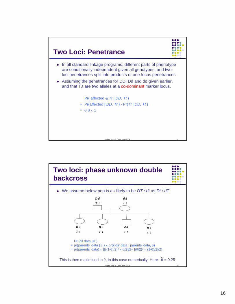
Log (base 10) odds or LOD scores

Suppose pr(data | θ) is the likelihood function of a recombination fraction θ generated by some 'data', and pr(data | 1/2) is the same likelihood when θ= 1/2.Statistical theory tells us that the ratio

L = pr(data | θ*) / pr(data | 1/2) provides a basis for deciding whether θ =θ* rather than θ = 1/2.

This can equally well be done with Log10L, i.e.LOD(θ*) = Log10{pr(data | θ*) / pr(data | 1/2)}

measures the relative strength of the data for θ = θ* rather than θ = 1/2. Usually we write θ, not θ* and calculate the function LOD(θ).

© Eric Xing @ CMU, 2005-2009 34

Facts about/interpretation of LOD scores

1. Positive LOD scores suggests stronger support for θ* than for 1/2, negative LOD scores the reverse.

2. Higher LOD scores means stronger support, lower means the reverse.

3. LODs are additive across independent pedigrees, and under certain circumstances can be calculated sequentially.

4. For a single two-point linkage analysis, the threshold LOD ≈ 3 has become the de facto standard for "establishing linkage", i.e. rejecting the null hypothesis of no linkage.

5. When more than one locus or model is examined, the remark in 4 must be modified, sometimes dramatically.

18

© Eric Xing @ CMU, 2005-2009 35

Assumptions underpinning most 2-point human linkage analyses

Founder Frequencies: Hardy-Weinberg, random mating at each locus. Linkage equilibrium across loci, known allele frequencies; founders independent.Transmission: Mendelian segregation, no mutation.Penetrance: single locus, no room for dependence on relatives' phenotypes or environment. Known (including phenocopy rate).Implicit: phenotype and genotype data correct, marker order and location correctComment: Some analyses are robust, others can be very sensitive to violations of some of these assumptions. Non-standard linkage analyses can be developed.

© Eric Xing @ CMU, 2005-2009 36

Beyond two-point human linkage analysis

The real challenge is multipoint linkage analysis, but going there would take more time than we have today.

Next in importance is dealing with two-locus penetrances.

19

© Eric Xing @ CMU, 2005-2009 37

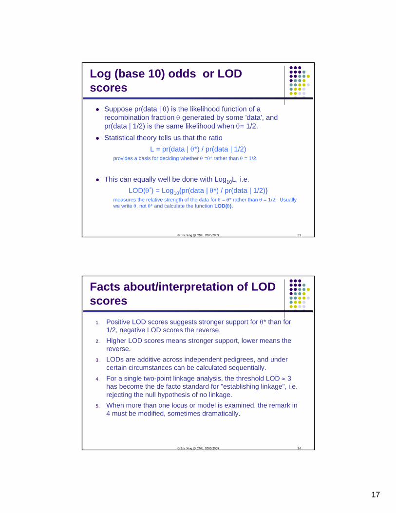
Nonparametric Methods for Linkage Analysis

© Eric Xing @ CMU, 2005-2009 38

Why Nonparametric Linkage Analysis?

Disadvantages of the LOD-score methodWhat if the model (allele frequency, penetrance etc.) is incorrect?Works well for single-locus and high-penetrance diseases, but many diseases are multifactorialData on large pedigrees are rare

Affected sib-pair analysisNonparametric method – no genetic modelData: Genotypes of affected pair of siblings and their parents

20

© Eric Xing @ CMU, 2005-2009 39

Affected Sib-Pair AnalysisIf the given genetic marker is linked to the disease locus, affected siblings share more identity-by-descent (IBD) alleles at the marker locus than expected. (i.e., affected siblings are likely to share the segment of the chromosome containing the disease locus.)

IBD (identity by descent) : Alleles are demonstrably copies of the same ancestral allele. IBS (identity by state) : Alleles look the same, but they are not derived from a known common ancestor

© Eric Xing @ CMU, 2005-2009 40

IBD and IBS

A1A3 A1A2

A1A1 A1A1

2 IBD, 2 IBS

A1A2 A2A3

A1A3 A1A2

1 IBD, 1IBS

A1A3 A2A3

A2A3 A1A3

0 IBD, 1 IBS

21

© Eric Xing @ CMU, 2005-2009 41

When There is No LinkageUnder the null hypothesis of no linkage between the marker locus and the disease locus (random segregation), the probabilities of a sib-pair sharing alleles IBD are given as:

P(0 IBD) = (1-0.5)*(1-0.5) = 0.25P(1 IBD) = 0.5*(1-0.5) + (1-0.5)*0.5 = 0.5P(2 IBD) = 0.5*0.5 = 0.25

Expected number of IBD alleles = 0*0.25+1*0.5+2*0.25 = 1

AB CD

Sib 1 Sib 2

AC (2 IBD)AD (1 IBD)BC (1 IBD)BD (0 IBD)

AC

© Eric Xing @ CMU, 2005-2009 42

When There is LinkageDominant disease

Pairs of siblings share one or two disease-related allelesExpected number of IBDs > 1

This can be detected in the linkage analysis

AB CD

Sib 1 Sib 2

AC (2 IBD)AD (1 IBD)

ACUnder the dominant disease model where A is linked to the disease locus, given Sib1 = (A,C), the only possible allele combinations for Sib2 are (A,C) or (A,D)

22

© Eric Xing @ CMU, 2005-2009 43

When There is LinkageRecessive disease

Pairs of siblings share both disease-related allelesExpected number of IBDs > 1

This can be detected in the linkage analysis

Parents are carriers

AB CD

Sib 1 Sib 2

AC (2 IBD)AC

Under the recessive disease model, given Sib1 = (A,C), the only possible allele combination for Sib2 is (A,C)

© Eric Xing @ CMU, 2005-2009 44

Data : genotypes of the pair of affected siblings and their parents

Two different approaches for hypothesis testingCompare the expected and observed frequency of siblings with 0, 1, and 2 IBDs under the null hypothesis H0 = (0.25, 0.5, 0.25)

χ2 test with 2 degrees of freedom

Compare the expected and observed average number of IBDs under the null hypothesis H0 = 1 (“mean test”)χ2 test with 1 degree of freedom

Note: we do not make assumptions on the genetics of disease (dominant or recessive)

Affected Sib-Pair Analysis

23

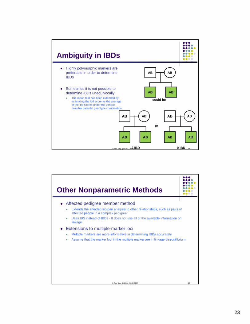
© Eric Xing @ CMU, 2005-2009 45

Ambiguity in IBDsHighly polymorphic markers are preferable in order to determine IBDs

Sometimes it is not possible to determine IBDs unequivocally

The mean test has been extended by estimating the ibd score as the average of the ibd scores under the various possible parental genotype combination

AB AB

AB AB

could be

AB AB

AB AB

0 IBD

AB AB

AB AB

2 IBD

or

© Eric Xing @ CMU, 2005-2009 46

Other Nonparametric MethodsAffected pedigree member method

Extends the affected sib-pair analysis to other relationships, such as pairs of affected people in a complex pedigreeUses IBS instead of IBDs - It does not use all of the available information on linkage

Extensions to multiple-marker lociMultiple markers are more informative in determining IBDs accuratelyAssume that the marker loci in the multiple marker are in linkage disequilibrium

24

© Eric Xing @ CMU, 2005-2009 47

Acknowledgements

Melanie Bahlo, WEHIHongyu Zhao, Yale

Karl Broman, Johns HopkinsNusrat Rabbee, UCB

© Eric Xing @ CMU, 2005-2009 48

Referenceswww.netspace.org/MendelWeb

HLK Whitehouse: Towards an Understanding of the Mechanism of Heredity, 3rd ed. Arnold 1973

Kenneth Lange: Mathematical and statistical methods for genetic analysis, Springer 1997

Elizabeth A Thompson: Statistical inference from genetic data on pedigrees, CBMS, IMS, 2000.

Jurg Ott : Analysis of human genetic linkage, 3rd ednJohns Hopkins University Press 1999

JD Terwilliger & J Ott : Handbook of human genetic linkage, Johns Hopkins University Press 1994