COMPUTATIONAL FLUID DYNAMIC MODELING TO IMPROVE THE

A Resource for the State of Florida

HURRICANE LOSS REDUCTION

FOR HOUSING IN FLORIDA:

COMPUTATIONAL FLUID DYNAMIC MODELING TO IMPROVE THE PERFORMANCE

OF THE WALL OF WIND

A Research Project Funded by The State of Florida Division of Emergency Management

Through Contract # 06RC-A%-13-00-05-261

Prepared by:

R. Panneer Selvam, Ph.D., PE James T. Womble Professor of Computational Mechanics and Nanotechnology Modeling

& Mita Sarkar MSCE, Graduate Student

Department of Civil Engineering, University of Arkansas

In Partnership with: The International Hurricane Research Center

Florida International University

August 2007

2

Computational Fluid Dynamic Modeling to Improve the Performance of Wall of Wind

Executive Summary A turbulence simulation system to reproduce conditions in the Atmospheric Boundary Layer (ABL) is needed to improve the performance of the Wall of Wind (WOW) full-scale testing apparatus. This can be achieved by using a system of rudders located directly in front of the propellers that are controlled and moved within a certain range to create turbulence. A computational fluid dynamics (CFD) analysis is needed to determine the configuration of the WOW system including the size of the rudders and the range of motion necessary to create such turbulence conditions. The below stated research is the first phase of the CFD analysis. 1. Turbulence Generation Using the Airfoil The flow around the airfoil is discretized using 161x72 grid system as shown in Fig. 1. The dimensions are non-dimensionalized with respect to the width of the chord B and the upstream velocity V. The airfoil is rotated using the non-dimensional reduced velocity u* = V/wB where w is the frequency of the airfoil rotation in radians/second. The airfoil is rotated about 0.3 units from the left edge. At this time the u* is considered to be 1.2 which is close to a period of 0.1 sec for a wind speed of 110 mph and a chord length of 25 inches. The time step used for the computer runs are 0.002 non-dimensional time. The numerical procedure used to compute the flow around the moving airfoil is similar to the one reported in Selvam et al. (2002a & b).The turbulence generated on the leeward side about 1 airfoil width from the tail of the airfoil is considered for comparison. The airfoil is rotated using a sine function with different amplitudes and frequencies.

Fig. 1: Velocity vector around the airfoil. The spacing shows the grid configuration. 1.1 Effect of Amplitude of Rotation on Turbulence Generation The maximum amplitude of the rotation is considered to be 6, 11 and 15 degrees and the frequency is kept constant ie u*=1.2. The predicted velocity in the x and y directions and the

3

corresponding amplitude of velocity for different frequencies are plotted in Fig. 1.1.1 and Fig. 1.1.2. The number of frequencies considered in the frequency domain is 40 and the computer model was run for 30 non-dimensional time units or 15000 time steps. From the figure one can see that maximum amplitudes increased from 0.08 to 0.1 in the x-direction and 0.06 to 0.17 in the y-direction. The magnitude of the high frequencies also increased. In the y-direction for higher angle of rotation there is a definite pattern of increase in the amplitude for high frequencies.

4

(a) Vx and Vy for 6 degrees

(b) Vx and Vy for 11 degrees

(c) Vx and Vy for 15 degrees

Fig. 1.1.1: Velocity plot in the x and y directions for 6, 11 and 15 degrees

5

(a)Velocity amplitudes in x and y for 6 degrees

(b) Velocity amplitudes in x and y for 11 degrees

(c) Velocity amplitudes in x and y for 15 degrees

Fig. 1.1.2: Amplitude for different frequencies in the x and y directions for 6, 11 and 15 degrees

6

(a) Velocity spectra in the x and y direction for 6 degrees

(b) Velocity spectra in the x and y direction for 11 degrees

(c) Velocity spectra in the x and y direction for 15 degrees

Fig. 1.1.3: Turbulent spectra plot in the x and y direction for 6, 11 and 15 degrees

7

1.2 Effect of Frequency on the Turbulence Generation To study the effect of frequency on turbulence generation the amplitude of the motion of the airfoil is kept at 15 degrees. The u* which is related to frequency is varied from 0.9 to 1.5. These runs are compared with results from the previous section runs for u*=1.2. In these runs it is found that when a time step of 0.002 is used the solution diverged. Next runs were made with 0.001 and results showed a converged solution. The computer generated velocities in the x and y directions and the corresponding amplitudes and spectral density for various frequencies are plotted in Fig. 1.2.1 to Fig. 1.2.3. It was found that for a higher u* (=1.5) the high frequency turbulence are far more developed than for lower u* values.

8

(a) Vx and Vy for u*=0.9

(b) Vx and Vy for u*=1.2

(c) Vx and Vy for u*=1.5

Fig. 1.2.1: Velocity plot in the x and y directions for reduced velocity u* of 0.9 and 1.5

9

(a) Velocity amplitudes in x and y for u*=0.9

(b) Velocity amplitudes in x and y for u*=1.2

(c) Velocity amplitudes in x and y for u*=1.5

Fig. 1.2.2: Amplitude for different frequencies in the x and y directions for reduced velocity u* of 0.9 and 1.5

10

(a) Velocity spectra in the x and y direction for u*=0.9

(b) Velocity spectra in the x and y direction for u*=1.2

(c) Velocity spectra in the x and y direction for u*=1.5

Fig. 1.2.3: Turbulent spectra plot in the x and y direction for reduced velocity u* of 0.9 and 1.5

11

2. Contraction Design for the Wall of Wind 2.1. Contraction design of WOW when units have constant cross section and parallel to each other Each Wall of Wind unit is comprised of three sections including the propeller, engine and diffuser. There are six Wall of Wind units in total. Every unit is 8 foot which is equal to 1 unit in computational length scale. The wind is flowing through each unit from left to right (along X axis). The unit (flow region) separating wall thickness is 0.015 (1.44 inches) units. There is mixing zone of 4 foot (0.5 units) in width below and above the fluid flow zones (unit) and right side of the fluid flow zone. The details of dimensions are shown in Fig. 2.1.

Fig. 2.1: Dimension details of domain

Four different cases were considered for this study:

• Case 1- units with out any gap between one unit to next;

• Case 2 - units with gap width 4.3 inches (0.045 units);

32’6”

20’

9.6’4.8’

3 units @ 8’ each

1 6’

4’

4’

12

• Case 3: units with gap width 10.1 inches (0.105 units);

• Case 4: units with gap width 2 foot (0.25 units).

Grid details were the same for all the cases. The smallest grid length along X axis and Y axis was 0.025 (2.4 inches) and 0.0075 (0.72 inches) units respectively. In the X-direction a uniform mesh length is used and in Y-direction a non-uniform mesh length is used. Smaller grids are used in and around the unit separating wall and gaps. The flow details for Case 1 to Case 4 are shown in Fig. 2.1.1 to Fig. 2.1.4 respectively. To get an idea about the volumetric flow rate or discharge in each unit before exit of unit, it is calculated at a distance of x = 1.95 units (15.6 foot) for every case and tabulated in Table 2.1.1.

Fig. 2.1.1.d. Zoomed view of velocity

vector in and around upper most gap Fig. 2.1.1.e. Zoomed view of velocity vector in and around lower most gap

Fig. 2.1.1.a. U-velocity contour Fig. 2.1.1.b. Pressure contour Fig. 2.1.1.c. Velocity vector with pressure contour legend

13

Fig. 2.1.1: Details of fluid flow in Units with out gap between neighboring units (Case 1)

Fig. 2.1.1.f. Zoomed view of velocity vector around upper gap of middle unit

Fig. 2.1.1.g. Zoomed view of velocity vector around lower gap of middle unit

Fig. 2.1.1.h. U velocity distribution along Y direction at the starting of gap (at x = 0.625 units)

Fig. 2.1.1.i. U velocity distribution along Y direction just before ending of gap (at x = 0.775 units)

Fig. 2.1.1.j. U velocity distribution along Y direction just before unit exit (at x = 1.95 units)

Fig. 2.1.1.k. U velocity distribution along Y direction just after unit exit (at x = 2.05 units)

14

Fig. 2.1.2.d. Zoomed view of velocity vector in and around the upper most gap

Fig. 2.1.2.e. Zoomed view of velocity vector in and around the lower most gap

Fig. 2.1.2.f. Zoomed view of velocity vector in around upper gap of middle unit

Fig. 2.1.2.g. Zoomed view of velocity vector in and around lower gap of middle unit

Fig. 2.1.2.a. U-velocity contour

Fig. 2.1.2.b. Pressure contour

Fig. 2.1.2.c. Velocity vector diagram with pressure contour legend

15

Fig.2.1.2: Details of fluid flow in units with gap between neighboring units for gap width 4.3 inch (0.045 units) (Case 2)








16


Fig. 2.1.3.e. Zoomed view of velocity vector in and around the lower most gap

Fig. 2.1.3.f. Zoomed view of velocity vector in and around the upper gap of middle unit

Fig. 2.1.3.g. Zoomed view of velocity vector in and around the lower gap of middle unit



17

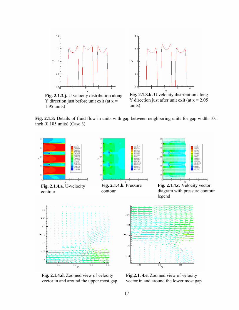
Fig. 2.1.3: Details of fluid flow in units with gap between neighboring units for gap width 10.1 inch (0.105 units) (Case 3)







Fig.2.1. 4.e. Zoomed view of velocity vector in and around the lower most gap

18

Fig. 2.1.4: Details of fluid flow in units with gap between neighboring units for gap width 2 foot (0.25 units) (Case 4)

Fig. 2.1.4.f. Zoomed view of velocity vector in and around the upper gap of middle unit

Fig. 2.1.4.g. Zoomed view of velocity vector in and around the lower gap of middle unit





19

From the pressure diagram and velocity vector for Case 1 (Fig.2.1.1.b-c), it is found that there is interaction between one Wall of Wind unit to the next. The velocity and pressure distribution (Fig.2.1.1.a-b) is similar in the two end units but it is different in middle unit. To understand the interactions between each Wall of Wind units the U (horizontal) velocity component distribution across the units at different x distances are drawn (Fig.2.1.1.h-k) and the zoomed view of velocity vector around the gaps are seen (Fig.2.1.1.d-g). Fig.2.1.1.d shows the zoomed view of velocity vector in and around the upper most gap and from this figure it is seen that a portion of air is going to mixing zone from the upper unit through the upper gap. It is also found that the air is going out from the lower unit to lower mixing zone (Fig.2.1.1.e). From Fig.2.1.1.f-g it is seen that at the start of the gap, wind is coming inside from both neighboring units due to boundary layer formation and interacting inside the gap and going out towards both units. It is further found that the discharge just before the exit from the unit is higher for the middle unit whereas it is less for the two end units (Table 2.1.1) which may be due to the flow from the end units to the mixing zone.

Case 2 is showing the effect of a smaller gap (gap width 4.3 inch) between each Wall of Wind unit. Comparing the Fig.2.1.1 and Fig.2.1.2, it is found that the smaller gap does not have significant effects on the interaction between one unit to next. The results for Case 2 are quite similar with Case 1. From these results it can be concluded that a smaller gap does not have significant effect on the interaction between Wall of Wind units.

Case 3 shows the effect of a gap width of 10.1 inches. Fig.2.1.3.a-k shows the flow details for this case. The gap is reducing the interaction between units and it is reducing the velocity in neighboring units. The wind is coming from neighboring units through the gaps and it is increasing the velocity within the gap and decreasing the velocity in the Wall of Wind units (Fig.2.1.3.f-g). From the zoomed view of the velocity vector of middle unit (Fig.2.1.3.f-g) it is clear that the velocity is higher in the gap and from the U velocity distribution at the starting of gap. In Fig.2.1.3.h-i, it is evident that the velocity in every unit is lesser after the gap. For this case the U velocity distribution just before exit of the unit is not same in every unit. The velocity is higher in middle unit than end units results volumetric flow rate higher in middle unit (Table 1).

Case 4 shows the effect of a gap width of 2 foot. Fig.2.1.4.a-k shows the flow details for this case. The gap effectively reduces the interaction between units and the U velocity in neighboring units. The wind is coming from the neighboring units through the gaps, thereby increasing the velocity in the gap and decreasing the velocity in units (Fig.2.1.4.f-g). From the zoomed view of velocity vector in and around the upper and lower gap of the middle unit (Fig.2.1.4.f-g) it is clear that the velocity is higher in gap. From the U velocity distribution at starting of gap and just before ending of gap (Fig.2.1.4.h-i), it is seen that the velocity in every unit is lesser after the gap. For this case the U velocity distribution just before exit of the unit is almost same in every unit (Fig.2.1.4.j). In addition the measured volumetric flow rate in every unit at the exit is almost same (Table 2.1.1).

20

Table 2.1.1: Calculated volumetric flow rate (discharge) just before exit of units (at x = 1.95 i.e. 16.5 ft) for different conditions

Unit 1 (lower) Unit 2 (middle) Unit 3 (upper) Case 1 (with out gap) 0.986 0.997 0.986 Case 2 (gap width 4.3 inch (0.045 units))

0.986 0.997 0.986

Case 3 (gap width 10 inch (0.105 units))

0.980 0.994 0.980

Case 4 (gap width 2 foot (0.25 units)) 0.969 0.968 0.969

Conclusions: 1. When there is no gap between neighboring units limited interaction exists. The flow

coming from lower and middle unit to the gap in between these two units and again going out from gap to these units and in this interaction process the U velocity is reduced in unit from 1.13 to 1.09 units (maximum U velocity). Similar interaction happens to the middle and upper units. The flow goes out from lower unit and upper unit to lower and upper mixing zone respectively through the gaps,

2. The gap between neighboring units reduces the interaction between one unit to next but interaction is there between unit and gap (Fig. 2.1.4.f-g). The higher gap width (gap with ≥ 10 inches) reduces the volumetric flow rate (discharge) in every unit (Table 1).

3. For lesser gap width (gap width < 10 inches) the flow pattern is similar to no gap between neighboring units’ case (comparing Fig.2.1.1 & Fig.2.1.2).

4. The volumetric flow rate (discharge) in each unit decreases with the increase in gap width (Table 2.1.1). The discharge decreases from 0.997 units to 0.969 units due to the increase in gape width from 0.0 to 0.25 units.

5. When the gap width is 25% (0.25 units) of unit width, the volumetric flow rate (discharge) in every unit is almost same as 0.969 units (Table 2.1.1).

2.2 Contraction design of WOW when the units are diffuser type: Every unit’s exit width is 8 foot which is equal to 1 unit in computational length scale. The wind is flowing through each unit from left to right (along X axis). There is mixing zone of around 4 foot (0.5 units) in width below and above the unit region. Right side of the unit region 8 foot space is considered for mixing and to develop the uniform flow. Fig. 2.2.1 shows the details of actual units’ orientation and length and exact unit orientation is used for computer model.

21

Fig.2.2.1: Details of contraction design domain

The U velocity component (velocity parallel to X axis) contour, pressure contour and velocity vector diagram are shown in Fig.2.2.2-2.2.4. Fig.2.2.5.a-d shows the zoomed view of velocity vector at different positions. It is found that the air coming from different unit is mixing in mixing region after exiting from the units. From the upper and lower unit, the wind is coming toward middle unit (Fig.2.2.3-4). From U velocity contour plot it is also found that at the right end of computational domain the wind velocity is more uniform (Fig.2.2.3). To see the mixing in more detail and conclude further the u, v velocity component and pressure contour will be plotted at different position along the units.

22

Fig.2.2.4: Velocity vector diagram with u-velocity contour legend

Fig.2.2.2: Pressure contour plot Fig.2.2.3: U velocity contour plot

23

Fig.2.2.5.d: Zoomed view of velocity vector at and around the exit of units

References

1. Selvam, R.P., Govindaswamy, S. and Bosch, H., Aeroelastic analysis of bridges using FEM and moving grids, Wind & Structures, Vol. 5, pp. 257-266, 2002a

2. Selvam, R.P., Computer modeling for bridge aerodynamics (invited paper), in Wind Engineering, by K. Kumar (Ed), Phoenix Publishing House, New Delhi, India, 2002b, pp. 11-25 .

Fig. 2.2.5.a. Zoomed view of velocity vector inside the lower unit

Fig. 2.2.5.b. Zoomed view of velocity vector inside the middle unit

Fig. 2.2.5.c. Zoomed view of velocity vector inside the upper unit

Documents

COMPUTATIONAL FLUID DYNAMIC MODELING TO IMPROVE THE