Computational Cosmology: From the Early Universe to … · Computational Cosmology: From the Early Universe to the Large Scale Structure 7 1 Introduction Numerical investigations

Computational Cosmology: From the Early Universe to the

Large Scale Structure

Peter AnninosUniversity of California

Lawrence Livermore National Laboratory7000 East Ave.

Livermore, CA 94550-9234U.S.A.

email: [email protected]

Accepted on 15 February 2001

Published on 20 March 2001

http://www.livingreviews.org/lrr-2001-2

Living Reviews in RelativityPublished by the Max Planck Institute for Gravitational Physics

Albert Einstein Institute, Germany

Abstract

In order to account for the observable Universe, any comprehensive theory or model ofcosmology must draw from many disciplines of physics, including gauge theories of strongand weak interactions, the hydrodynamics and microphysics of baryonic matter, electromag-netic fields, and spacetime curvature, for example. Although it is difficult to incorporate allthese physical elements into a single complete model of our Universe, advances in computingmethods and technologies have contributed significantly towards our understanding of cosmo-logical models, the Universe, and astrophysical processes within them. A sample of numericalcalculations (and numerical methods) applied to specific issues in cosmology are reviewed inthis article: from the Big Bang singularity dynamics to the fundamental interactions of grav-itational waves; from the quark-hadron phase transition to the large scale structure of theUniverse. The emphasis, although not exclusively, is on those calculations designed to testdifferent models of cosmology against the observed Universe.

c©Max Planck Society and the authors.Further information on copyright is given at

http://relativity.livingreviews.org/Info/Copyright/For permission to reproduce the article please contact [email protected].

http://relativity.livingreviews.org/Info/Copyright/

How to cite this article

Owing to the fact that a Living Reviews article can evolve over time, we recommend to cite thearticle as follows:

Peter Anninos,“Computational Cosmology: From the Early Universe to the Large Scale Structure”,

Living Rev. Relativity, 4, (2001), 2. [Online Article]: cited [<date>],http://www.livingreviews.org/lrr-2001-2

The date given as <date> then uniquely identifies the version of the article you are referring to.

Article Revisions

Living Reviews supports two different ways to keep its articles up-to-date:

Fast-track revision A fast-track revision provides the author with the opportunity to add shortnotices of current research results, trends and developments, or important publications tothe article. A fast-track revision is refereed by the responsible subject editor. If an articlehas undergone a fast-track revision, a summary of changes will be listed here.

Major update A major update will include substantial changes and additions and is subject tofull external refereeing. It is published with a new publication number.

For detailed documentation of an article’s evolution, please refer always to the history documentof the article’s online version at http://www.livingreviews.org/lrr-2001-2.

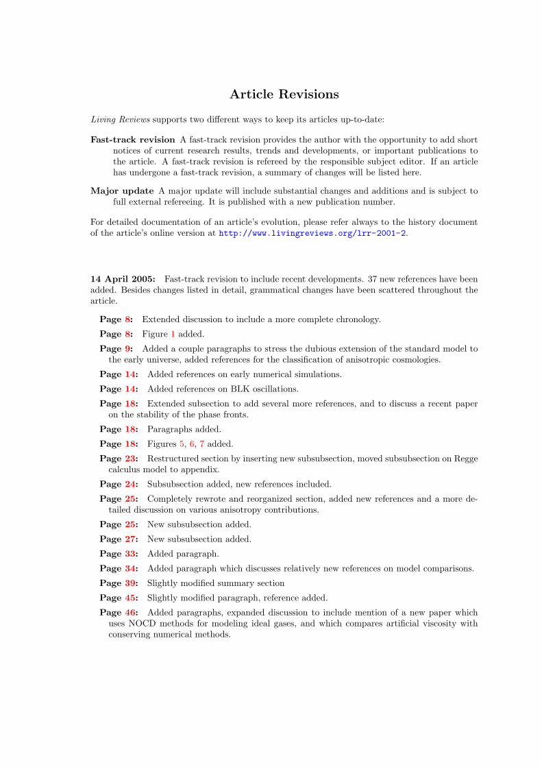
14 April 2005: Fast-track revision to include recent developments. 37 new references have beenadded. Besides changes listed in detail, grammatical changes have been scattered throughout thearticle.

Page 8: Extended discussion to include a more complete chronology.

Page 8: Figure 1 added.

Page 9: Added a couple paragraphs to stress the dubious extension of the standard model tothe early universe, added references for the classification of anisotropic cosmologies.

Page 14: Added references on early numerical simulations.

Page 14: Added references on BLK oscillations.

Page 18: Extended subsection to add several more references, and to discuss a recent paperon the stability of the phase fronts.

Page 18: Paragraphs added.

Page 18: Figures 5, 6, 7 added.

Page 23: Restructured section by inserting new subsubsection, moved subsubsection on Reggecalculus model to appendix.

Page 24: Subsubsection added, new references included.

Page 25: Completely rewrote and reorganized section, added new references and a more de-tailed discussion on various anisotropy contributions.

Page 25: New subsubsection added.

Page 27: New subsubsection added.

Page 33: Added paragraph.

Page 34: Added paragraph which discusses relatively new references on model comparisons.

Page 39: Slightly modified summary section

Page 45: Slightly modified paragraph, reference added.

Page 46: Added paragraphs, expanded discussion to include mention of a new paper whichuses NOCD methods for modeling ideal gases, and which compares artificial viscosity withconserving numerical methods.


Page 47: New section added to include the stress tensor for nonideal fluids with shear stress.

Page 49: Reorganized section by adding new subsubsection, added example of a typical chem-ical network useful for primordial cosmology.

Page 51: Reorganized section by adding new subsubsection, added reference.

Contents

1 Introduction 7

2 Background 82.1 A brief chronology . . . . . . . . . . . . . . . . . . . . . . . . . . . . . . . . . . . . 82.2 The standard model . . . . . . . . . . . . . . . . . . . . . . . . . . . . . . . . . . . 9

3 Relativistic Cosmology 133.1 Singularities . . . . . . . . . . . . . . . . . . . . . . . . . . . . . . . . . . . . . . . . 13

3.1.1 Mixmaster dynamics . . . . . . . . . . . . . . . . . . . . . . . . . . . . . . . 133.1.2 AVTD vs. BLK oscillatory behavior . . . . . . . . . . . . . . . . . . . . . . 14

3.2 Inflation . . . . . . . . . . . . . . . . . . . . . . . . . . . . . . . . . . . . . . . . . . 153.2.1 Plane symmetry . . . . . . . . . . . . . . . . . . . . . . . . . . . . . . . . . 153.2.2 Spherical symmetry . . . . . . . . . . . . . . . . . . . . . . . . . . . . . . . 153.2.3 Bianchi V . . . . . . . . . . . . . . . . . . . . . . . . . . . . . . . . . . . . . 163.2.4 Gravitational waves + cosmological constant . . . . . . . . . . . . . . . . . 163.2.5 3D inhomogeneous spacetimes . . . . . . . . . . . . . . . . . . . . . . . . . 16

3.3 Chaotic scalar field dynamics . . . . . . . . . . . . . . . . . . . . . . . . . . . . . . 163.4 Quark-hadron phase transition . . . . . . . . . . . . . . . . . . . . . . . . . . . . . 183.5 Nucleosynthesis . . . . . . . . . . . . . . . . . . . . . . . . . . . . . . . . . . . . . . 223.6 Cosmological gravitational waves . . . . . . . . . . . . . . . . . . . . . . . . . . . . 23

3.6.1 Planar symmetry . . . . . . . . . . . . . . . . . . . . . . . . . . . . . . . . . 233.6.2 Multi-dimensional vacuum cosmologies . . . . . . . . . . . . . . . . . . . . . 24

4 Physical Cosmology 254.1 Cosmic microwave background . . . . . . . . . . . . . . . . . . . . . . . . . . . . . 25

4.1.1 Primordial black body effects . . . . . . . . . . . . . . . . . . . . . . . . . . 254.1.2 Primary anisotropies . . . . . . . . . . . . . . . . . . . . . . . . . . . . . . . 274.1.3 Secondary anisotropies . . . . . . . . . . . . . . . . . . . . . . . . . . . . . . 274.1.4 Computing CMBR anisotropies with ray-tracing methods . . . . . . . . . . 29

4.2 Gravitational lensing . . . . . . . . . . . . . . . . . . . . . . . . . . . . . . . . . . . 314.3 First star formation . . . . . . . . . . . . . . . . . . . . . . . . . . . . . . . . . . . 314.4 Lyα forest . . . . . . . . . . . . . . . . . . . . . . . . . . . . . . . . . . . . . . . . . 334.5 Galaxy clusters . . . . . . . . . . . . . . . . . . . . . . . . . . . . . . . . . . . . . . 34

4.5.1 Internal structure . . . . . . . . . . . . . . . . . . . . . . . . . . . . . . . . . 344.5.2 Number density evolution . . . . . . . . . . . . . . . . . . . . . . . . . . . . 364.5.3 X-ray luminosity function . . . . . . . . . . . . . . . . . . . . . . . . . . . . 364.5.4 SZ effect . . . . . . . . . . . . . . . . . . . . . . . . . . . . . . . . . . . . . . 37

4.6 Cosmological sheets . . . . . . . . . . . . . . . . . . . . . . . . . . . . . . . . . . . 37

5 Summary 39

6 Appendix: Basic Equations and Numerical Methods 406.1 The Einstein equations . . . . . . . . . . . . . . . . . . . . . . . . . . . . . . . . . . 40

6.1.1 ADM formalism . . . . . . . . . . . . . . . . . . . . . . . . . . . . . . . . . 406.1.2 Kinematic conditions . . . . . . . . . . . . . . . . . . . . . . . . . . . . . . . 416.1.3 Symplectic formalism . . . . . . . . . . . . . . . . . . . . . . . . . . . . . . 426.1.4 Regge calculus model . . . . . . . . . . . . . . . . . . . . . . . . . . . . . . 42

6.2 Sources of matter . . . . . . . . . . . . . . . . . . . . . . . . . . . . . . . . . . . . . 436.2.1 Cosmological constant . . . . . . . . . . . . . . . . . . . . . . . . . . . . . . 43

6.2.2 Scalar field . . . . . . . . . . . . . . . . . . . . . . . . . . . . . . . . . . . . 436.2.3 Collisionless dust . . . . . . . . . . . . . . . . . . . . . . . . . . . . . . . . . 446.2.4 Ideal gas . . . . . . . . . . . . . . . . . . . . . . . . . . . . . . . . . . . . . . 456.2.5 Imperfect fluid . . . . . . . . . . . . . . . . . . . . . . . . . . . . . . . . . . 47

6.3 Constrained nonlinear initial data . . . . . . . . . . . . . . . . . . . . . . . . . . . . 476.4 Newtonian limit . . . . . . . . . . . . . . . . . . . . . . . . . . . . . . . . . . . . . . 48

6.4.1 Dark and baryonic matter equations . . . . . . . . . . . . . . . . . . . . . . 486.4.2 Primordial chemistry . . . . . . . . . . . . . . . . . . . . . . . . . . . . . . . 496.4.3 Numerical methods . . . . . . . . . . . . . . . . . . . . . . . . . . . . . . . . 516.4.4 Linear initial data . . . . . . . . . . . . . . . . . . . . . . . . . . . . . . . . 51

References 53

Computational Cosmology: From the Early Universe to the Large Scale Structure 7

1 Introduction

Numerical investigations of cosmological spacetimes can be categorized into two broad classesof calculations, distinguished by their computational goals: (i) geometrical and mathematicalprinciples of cosmological models, and (ii) physical and astrophysical cosmology. In the former,the emphasis is on the geometric framework in which astrophysical processes occur, for examplecosmological expansion, topological singularities, geometrodynamics in general, and classificationcharacteristics or invariants of the many models allowed by the theory of general relativity. In thelatter, the emphasis is on the cosmological and astrophysical processes in the real or observableUniverse, and the quest to determine the model which best describes our Universe. The former ispure in the sense that it concerns the fundamental nonlinear behavior of the Einstein equations andthe gravitational field. The latter is more complex as it addresses the composition, organization,and dynamics of the Universe from the small scales (fundamental particles and elements) to thelarge (galaxies and clusters of galaxies). However the distinction is not always so clear, andgeometric effects in the spacetime curvature can have significant consequences for the evolutionand observation of matter distributions.

Any comprehensive model of cosmology must therefore include nonlinear interactions betweendifferent matter sources and spacetime curvature. A realistic model of the Universe must alsocover large dynamical spatial and temporal scales, extreme temperature and density distributions,and highly dynamic atomic and molecular matter compositions. In addition, due to all the variedphysical processes of cosmological significance, one must draw from many disciplines of physics tomodel curvature anisotropies, gravitational waves, electromagnetic fields, nucleosynthesis, particlephysics, hydrodynamic fluids, etc. These phenomena are described in terms of coupled nonlinearpartial differential equations and must be solved numerically for general inhomogeneous spacetimes.The situation appears extremely complex, even with current technological and computational ad-vances. As a result, the codes and numerical methods that have been developed to date are designedto investigate very specific problems with either idealized symmetries or simplifying assumptionsregarding the metric behavior, the matter distribution/composition or the interactions among thematter types and spacetime curvature.

It is the purpose of this article to review published numerical cosmological calculations address-ing problems from the very early Universe to the present; from the purely geometrical dynamics ofthe initial singularity to the large scale structure of the Universe. There are three major sections:Section 2 where a brief overview is presented of various defining events occurring throughout thehistory of our Universe and in the context of the standard model, Section 3 where reviews of earlyUniverse and relativistic cosmological calculations are presented, and Section 4 which focuses onstructure formation in the post-recombination epoch and on testing cosmological models againstobservations. Following the summary paragraphs in Section 5, an appendix in Section 6 presentsthe basic Einstein equations, kinematic considerations, matter source equations with curvature,and the equations of perturbative physical cosmology on background isotropic models. Referencesto numerical methods are also supplied and reviewed for each case.

Living Reviews in Relativityhttp://www.livingreviews.org/lrr-2001-2


8 Peter Anninos

2 Background

2.1 A brief chronology

With current observational constraints, the physical state of our Universe, as understood in thecontext of the standard or Friedman–Lemaıtre–Robertson–Walker (FLRW) model, can be crudelyextrapolated back to ∼ 10−43 seconds after the Big Bang, before which the classical descriptionof general relativity is expected to give way to a quantum theory of gravity. As the time-line inFigure 1 shows, the Universe was a plasma of relativistic particles at the earliest times consistingof quarks, leptons, gauge bosons, and Higgs bosons represented by scalar fields with interactionand symmetry regulating potentials.

nucsyn

GUTgaugebosons

quarksgluonsleptons

neutronsprotonselectronsneutrinos

hydrogendeuteriumheliumlithium

structureformationstarts

starsgalaxiesclusters

-43 -34 -11 -5 1 11 13 17

31 26 15 13 10 5 4 0

28 23 11 8 6 1 0 -3

Planckera

Lepton/Quarkera

Radiationera

Matterera

n,p

ν

n,p

γ

R~t^1/2R~t^2/3

quantumgravity

Log(t,sec)

Log(E,ev)

Log(T,K)

,γ

EW SSB QH SSB mat dom decoupling present

Log(R)

inflation

Figure 1: A historical time-line showing the major evolutionary stages of our Universe accordingto the standard model, from the earliest moments of the Planck era to the present. The horizontalaxis represents logarithmic time in seconds (or equivalently energy in electron-Volts or temperaturein Kelvin), and the solid red line roughly models the radius of the Universe, showing the differentrates of expansion at different times: exponential during inflation, shallow power law during theradiation dominated era, and a somewhat steeper power law during the current matter dominatedphase.

It is believed that several spontaneous symmetry breaking (SSB) phase transitions occured inthe early Universe as it expanded and cooled, including the grand unification transition (GUT) at∼ 10−34 s after the Big Bang in which the strong nuclear force split off from the weak and electro-magnetic forces (this also marks an era of inflationary expansion and the origin of matter-antimatterasymmetry through baryon, charge conjugation, and charge + parity violating interactions andnonequilibrium effects); the electroweak (EW) SSB transition at ∼ 10−11 s when the weak nuclearforce split from the electromagnetic force; and the chiral or quantum chromodynamic (QCD) sym-metry breaking transition at ∼ 10−5 s during which quarks condensed into hadrons. The most




stable hadrons (baryons, or protons and neutrons comprised of three quarks) survived the subse-quent period of baryon-antibaryon annihilations, which continued until the Universe cooled to thepoint at which new baryon-antibaryon pairs could no longer be produced. This resulted in a largenumber of photons and relatively few surviving baryons. Topological defects, defined as stableconfigurations of matter in the symmetric (high temperature) phase, may persist after any of thephase transitions described above to influence the subsequent evolution of matter structures. Thenature of the defects is determined by the phase transition and the symmetry properties of thematter, and some examples include domain walls, cosmic strings, monopoles, and textures.

A period of primordial nucleosynthesis followed from ∼ 10−2 to ∼ 102 s during which light ele-ment abundances were synthesized to form 24% helium with trace amounts of deuterium, tritium,helium-3, and lithium. Observations of these relative abundances represent the earliest confirma-tion of the standard model. It is also during this stage that neutrinos (produced from proton-protonand proton-photon interactions, and from the collapse or quantum evaporation/annihilation oftopological defects) stopped interacting with other matter, such as neutrons, protons, and pho-tons. Neutrinos that existed at this time separated from these other forms of matter and traveledfreely through the Universe at very high velocities, near the speed of light.

By ∼ 1011 s, the matter density became equal to the radiation density as the Universe con-tinued to expand, identifying the start of the current matter-dominated era and the beginningof structure formation. Later, at ∼ 1013 s (3 × 105 yr), the free ions and electrons combined toform atoms, effectively decoupling the matter from the radiation field as the Universe cooled. Thisdecoupling or post-recombination epoch marks the surface of last scattering and the boundary ofthe observable (via photons) Universe, and plays an important role in the history of the CosmicMicrowave Background Radiation (CMBR). Assuming a hierarchical Cold Dark Matter (CDM)structure formation scenario, the subsequent development of our Universe is characterized by thegrowth of structures with increasing size. For example, the first stars are likely to have formedat t ∼ 108y from molecular gas clouds when the Jeans mass of the background baryonic fluid wasapproximately 104M, as indicated in Figure 2. This epoch of pop III star generation is followedby the formation of galaxies at t ∼ 109 yr and subsequently galaxy clusters. Though somewhatcontroversial, estimates of the current age of our Universe range from 10 to 20 Gy, with a present-day linear structure scale radius of about 8h−1 Mpc, where h is the Hubble parameter (comparedto 2 – 3 Mpc typical for the virial radius of rich galaxy clusters).

2.2 The standard model

The isotropic and homogeneous FLRW cosmological model has been so successful in describingthe observable Universe that it is commonly referred to as the “standard model”. Furthermore,and to its credit, the model is relatively simple so that it allows for calculations and predictionsto be made of the very early Universe, including primordial nucleosynthesis at 10−2 seconds afterthe Big Bang, and even particle interactions approaching the Planck scale at 10−43 s. At present,observational support for the standard model includes:

• the expansion of the Universe as verified by the redshifts in galaxy spectra and quantified bymeasurements of the Hubble constant H0 = 100h km s−1 Mpc−1, where 0.5 ≤ h ≤ 1 is theHubble constant;

• the deceleration parameter observed in distant galaxy spectra (although uncertainties aboutgalactic evolution, intrinsic luminosities, and standard candles prevent an accurate estimate);

• the large scale isotropy and homogeneity of the Universe based on temperature anisotropymeasurements of the microwave background radiation and peculiar velocity fields of galaxies(although the light distribution from bright galaxies is somewhat contradictory);



10 Peter Anninos

Redshift

Log10(Time) years

Average Baryonic Jeans Mass

DMgravitationalinstability

negligible photon/matterinteraction

H2 coolinginstability

adiabatic

T=1eVisothermal

(1+z)^(3/2)

(1+z)^(−3/2)

CLUSTERS

GALAXIES

LYA CLOUDS

FIRST STARS

1000 200 100 20 10 5 1 0

1

2

3

4

5

6

7

8

9

10

11

12

13

14

Log10(J

ean

s m

ass

/M*)

hΩ Β

1/2

nH+ 10^(−5)−−− = −−−−−−−−nH h ΩΒ

5 8 9 107

Figure 2: Schematic depicting the general sequence of events in the post-recombination Universe.The solid and dotted lines potentially track the Jeans mass of the average baryonic gas componentfrom the recombination epoch at z ∼ 103 to the current time. A residual ionization fraction ofnH+/nH ∼ 10−4 following recombination allows for Compton interactions with photons to z ∼ 200,during which the Jeans mass remains constant at 105M. The Jeans mass then decreases as theUniverse expands adiabatically until the first collapsed structures form sufficient amounts of hydro-gen molecules to trigger a cooling instability and produce pop III stars at z ∼ 20. Star formationactivity can then reheat the Universe and raise the mean Jeans mass to above 108M. This reheat-ing could affect the subsequent development of structures such as galaxies and the observed Lyαclouds.




• the age of the Universe which yields roughly consistent estimates between the look-back timeto the Big Bang in the FLRW model and observed data such as the oldest stars, radioactiveelements, and cooling of white dwarf stars;

• the cosmic microwave background radiation suggests that the Universe began from a hotBig Bang and the data is consistent with a mostly isotropic model and a black body attemperature 2.7 K;

• CMBR precision measurements suggest best fit cosmological parameters in accord with thecritical density standard model;

• the abundance of light elements such as 2H, 3He, 4He, and 7Li, as predicted from the FLRWmodel, is consistent with observations, provides a bound on the baryon density and baryon-to-photon ratio, and is the earliest confirmation of the standard model;

• the present mass density, as determined from measurements of luminous matter and galacticrotation curves, can be accounted for by the FLRW model with a single density parameter(Ω0) to specify the metric topology;

• the distribution of galaxies and larger scale structures can be reproduced by numerical sim-ulations in the context of inhomogeneous perturbations of the FLRW models;

• the detection of dark energy from observations of supernovae is generally consistent withaccepted FLRW model parameters and cold dark matter + cosmological constant numericalstructure formation models.

Because of these remarkable agreements between observation and theory, most work in the fieldof physical cosmology (see Section 4) has utilized the standard model as the background spacetimein which the large scale structure evolves, with the ambition to further constrain parameters andstructure formation scenarios through numerical simulations. The most widely accepted form ofthe model is described by a set of dimensionless density parameters which sum to

Ωb + Ωd + Ωγ + ΩΛ = Ω0, (1)

where the different components measure the present mean baryon density Ωb, the dark matterdensity Ωd, the radiation energy Ωγ , and the dark energy ΩΛ. The relative contributions of eachsource and their sum Ω0 (which determines the topological curvature of the model) remains one ofthe most important issues in modern computational and observational cosmology. The reader isreferred to [104] for a more in-depth review of the standard model, and to [128, 154] for a summaryof observed cosmological parameter constraints and best fit “concordance” models. Peebles andRatra [133] provide a comprehensive literature survey and an excellent review of the standardmodel, cosmological tests, and the evidence for dark energy and the cosmological constant.

However, some important unanswered questions about the standard model concern the natureof the special conditions that produced an essentially geometrically flat Universe that is also ho-mogeneous and isotropic to a high degree over large scales. In an affort to address these questions,it should be noted that many other cosmological models can be constructed with a late time be-havior similar enough to the standard model that it is difficult to exclude them with absolutecertainty. Consider, for example, the collection of homogeneous but arbitrarily anisotropic vacuumspacetimes known as the Bianchi models [141, 69]. There are nine unique models in this familyof cosmologies, ranging from simple Bianchi I models representing the Kasner class of spacetimes(the flat FLRW model, sometimes referred to as Type I-homogeneous, belongs to this group),to the more complex and chaotic Bianchi IX or Mixmaster model (which also includes the closedFLRW model, Type IX-homogeneous). Several of these models will be discussed in the first section



12 Peter Anninos

on relativistic cosmology (Section 3) dealing pre-dominately with the early Universe, where themodels differ the most.

Anisotropic solutions, as well as more general (and in some cases exact) inhomogeneous cosmo-logical models with initial singularities, can isotropize through anisotropic damping mechanismsand adiabatic cooling by the expansion of the Universe to resemble the standard FLRW modelat late times. Furthermore, if matter is included in these spacetimes, the effective energy ofanisotropy, which generally dominates matter energy at early times, tends to become less impor-tant over time as the Universe expands. The geometry in these matter-filled anisotropic spacetimesthus evolves towards an isotropic state. Quantum mechanical effects have also been proposed as apossible anisotropy damping mechanism that takes place in the early Universe to convert vacuumgeometric energy to radiation energy and create particles. All of this suggests that the early timebehavior and effects of local and global geometry are highly uncertain, despite the fact that thestandard FLRW model is generally accepted as accurate enough for the late time description ofour Universe.

Further detailed information on homogeneous (including Bianchi) universes, as well as moregeneral classes of inhomogeneous cosmological models can be found in [105, 158, 70].




3 Relativistic Cosmology

This section is organized to track the chronological events in the history of the early or relativisticUniverse, focusing mainly on four defining moments: (i) the Big Bang singularity and the dynamicsof the very early Universe, (ii) inflation and its generic nature, (iii) QCD phase transitions, and (iv)primordial nucleosynthesis and the freeze-out of the light elements. The late or post-recombinationepoch is reserved to a separate Section 4.

3.1 Singularities

3.1.1 Mixmaster dynamics

Belinsky, Lifshitz, and Khalatnikov (BLK) [32, 33] and Misner [119] discovered that the Einsteinequations in the vacuum homogeneous Bianchi type IX (or Mixmaster) cosmology exhibit complexbehavior and are sensitive to initial conditions as the Big Bang singularity is approached. Inparticular, the solutions near the singularity are described qualitatively by a discrete map [30, 32]representing different sequences of Kasner spacetimes

ds2 = −dt2 + t2p1dx2 + t2p2dy2 + t2p3dz2, (2)

with time changing exponents pi, but otherwise constrained by p1 + p2 + p3 = p21 + p2

2 + p23 = 1.

Because this discrete mapping of Kasner epochs is chaotic, the Mixmaster dynamics is presumedto be chaotic as well.

Figure 3: Contour plot of the Bianchi type IX potential V , where β± are the anisotropy canonicalcoordinates. Seven level surfaces are shown at equally spaced decades ranging from 10−1 to 105.For large isocontours (V > 1), the potential is open and exhibits a strong triangular symmetrywith three narrow channels extending to spatial infinity. For V < 1, the potential closes and isapproximately circular for β± 1.

Mixmaster behavior can be studied in the context of Hamiltonian dynamics, with a Hamilto-nian [120]

2H = −p2Ω + p2

+ + p2− + e4α(V − 1), (3)



14 Peter Anninos

and a semi-bounded potential arising from the spatial scalar curvature (whose level curves areplotted in Figure 3)

V = 1 +13e−8β+ +

23e4β+

[cosh(4

√3β−)− 1

]− 4

3e−2β+ cosh(2

√3β−), (4)

where eα and β± are the scale factor and anisotropies, and pα and p± are the correspondingconjugate variables. A solution of this Hamiltonian system is an infinite sequence of Kasnerepochs with parameters that change when the phase space trajectories bounce off the potentialwalls, which become exponentially steep as the system evolves towards the singularity.

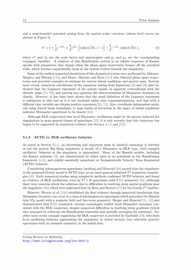
Some of the earliest numerical simulations of this dynamical system were performed by Matzner,Shepley, and Warren [116], and Moser, Matzner and Ryan [123] who followed phase space trajec-tories and provided examples of solutions for various initial conditions and special cases. Several,more recent, numerical calculations of the equations arising from Equations (3) and (4) have in-dicated that the Liapunov exponents of the system vanish, in apparent contradiction with thediscrete maps [53, 89], and putting into question the characterization of Mixmaster dynamics aschaotic. However, it has since been shown that the usual definition of the Liapunov exponentsis ambiguous in this case as it is not invariant under time reparametrizations, and that with adifferent time variable one obtains positive exponents [35, 73]. Also, coordinate independent meth-ods using fractal basin boundaries to map basins of attraction in the space of initial conditionsindicates Mixmaster spacetimes to be chaotic [64].

Although BLK conjectured that local Mixmaster oscillations might be the generic behavior forsingularities in more general classes of spacetimes [33], it is only recently that this conjecture hasbegun to be supported by numerical evidence (see Section 3.1.2 and [37]).

3.1.2 AVTD vs. BLK oscillatory behavior

As noted in Section 3.1.1, an interesting and important issue in classical cosmology is whetheror not the generic Big Bang singularity is locally of a Mixmaster or BLK type, with complexoscillatory behavior as the singularity is approached. Many of the Bianchi models, includingthe Kasner solutions (2), are characterized by either open or no potentials in the Hamiltonianframework [141], and exhibit essentially monotonic or Asymptotically Velocity Term Dominated(AVTD) behavior.

Considering inhomogeneous spacetimes, Isenberg and Moncrief [98] proved that the singularityin the polarized Gowdy model is AVTD type, as are more general polarized T 2 symmetric cosmolo-gies [38]. Early numerical studies using symplectic methods confirmed AVTD behavior and foundno evidence of BLK oscillations, even in T 3 × R spacetimes with U(1) symmetry [36] (althoughthere were concerns about the solutions due to difficulties in resolving steep spatial gradients nearthe singularity [36], which were addressed later by Hern and Stewart [87] for the Gowdy T 3 models).

However, Weaver et al. [160] established the first evidence through numerical simulations thatMixmaster dynamics can occur in a class of inhomogeneous spacetimes which generalize the Bianchitype VI0 model with a magnetic field and two-torus symmetry. Berger and Moncrief [41, 42] alsodemonstrated that U(1) symmetric vacuum cosmologies exhibit local Mixmaster dynamics con-sistent with the BLK conjecture, despite numerical difficulties in resolving steep gradients (whichthey managed by enforcing the Hamiltonian constraint and spatially averaging the solutions). An-other more recent example supporting the BLK conjecture is provided by Garfinkle [79], who findslocal oscillating behavior approaching the singularity in closed vacuum (but otherwise generic)spacetimes with no assumed symmetry in the initial data.




3.2 Inflation

The inflation paradigm is frequently invoked to explain the flatness (Ω0 ≈ 1 in the context of theFLRW model) and nearly isotropic nature of the Universe at large scales, attributing them to anera of exponential expansion at about 10−34 s after the Big Bang. This expansion acts as a strongdampening mechanism to random curvature or density fluctuations, and may be a generic attractorin the space of initial conditions. An essential component needed to trigger this inflationary phaseis a scalar or inflaton field φ representing spin zero particles. The vacuum energy of the field actsas an effective cosmological constant that regulates GUT symmetry breaking, particle creation,and the reheating of the Universe through an interaction potential V (φ) derived from the form ofsymmetry breaking that occurs as the temperature of the Universe decreases.

Early analytic studies focused on simplified models, treating the interaction potential as flatnear its local maximum where the field does not evolve significantly and where the formal analogyto an effective cosmological constant approximation is more precise. However, to properly accountfor the complexity of inflaton fields, the full dynamical equations (see Section 6.2.2) must beconsidered together with consistent curvature, matter and other scalar field couplings. Also, manydifferent theories of inflation and vacuum potentials have been proposed (see, for example, a recentreview by Lyth and Riotto [113] and an introductory article by Liddle [111]), and it is not likelythat simplified models can elucidate the full nonlinear complexity of scalar fields (see Section 3.3)nor the generic nature of inflation.

In order to study whether inflation can occur for arbitrary anisotropic and inhomogeneous data,many numerical simulations have been carried out with different symmetries, matter types andperturbations. A sample of such calculations is described in the following paragraphs.

3.2.1 Plane symmetry

Kurki-Suonio et al. [106] extended the planar cosmological code of Centrella and Wilson [59, 60] (seeSection 3.6.1) to include a scalar field and simulate the onset of inflation in the early Universe withan inhomogeneous Higgs field and a perfect fluid with a radiation equation of state p = ρ/3, wherep is the pressure and ρ is the energy density. Their results suggest that whether inflation occursor not can be sensitive to the shape of the potential φ. In particular, if the shape is flat enoughand satisfies the slow-roll conditions (essentially upper bounds on ∂V/∂φ and ∂2V/∂φ2 [104] nearthe false vacuum φ ∼ 0), even large initial fluctuations of the Higgs field do not prevent inflation.They considered two different forms of the potential: a Coleman–Weinberg type with interactionstrength λ and distance between true and false vacua σ

V (φ) = λφ4

[ln

(φ2

σ2

)− 1

2

]+λσ4

2, (5)

which is very flat near the false vacuum and does inflate; and a rounder “φ4” type

V (φ) = λ(φ2 − σ2)2, (6)

which, for their parameter combinations, does not.

3.2.2 Spherical symmetry

Goldwirth and Piran [83] studied the onset of inflation with inhomogeneous initial conditions forclosed, spherically symmetric spacetimes containing a massive scalar field and radiation field sources(described by a massless scalar field). In all the cases they considered, the radiation field dampsquickly and only an inhomogeneous massive scalar field remains to inflate the Universe. They findthat small inhomogeneities tend to reduce the amount of inflation and large initial inhomogeneities



16 Peter Anninos

can even suppress the onset of inflation. Their calculations indicate that the scalar field must have“suitable” initial values (local conditions for which an equivalent homogeneous Universe will inflate)over a domain of several horizon lengths in order to trigger inflation.

3.2.3 Bianchi V

Anninos et al. [14] investigated the simplest Bianchi model (type V) background that admitsvelocities or tilt in order to address the question of how the Universe can choose a uniform referenceframe at the exit from inflation, since the de Sitter metric does not have a preferred frame. Theyfind that inflation does not isotropize the Universe in the short wavelength limit. However, ifinflation persists, the wave behavior eventually freezes in and all velocities go to zero at least asrapidly as tanhβ ∼ R−1, where β is the relativistic tilt angle (a measure of velocity), and R is atypical scale associated with the radius of the Universe. Their results indicate that the velocitieseventually go to zero as inflation carries all spatial variations outside the horizon, and that theanswer to the posed question is that memory is retained and the Universe is never really de Sitter.

3.2.4 Gravitational waves + cosmological constant

In addition to the inflaton field, one can consider other sources of inhomogeneity, such as gravita-tional waves. Although linear waves in de Sitter space will decay exponentially and disappear, itis unclear what will happen if strong waves exist. Shinkai and Maeda [148] investigated the cosmicno-hair conjecture with gravitational waves and a cosmological constant (Λ) in 1D plane symmetricvacuum spacetimes, setting up Gaussian pulse wave data with amplitudes 0.02Λ ≤ max(

√I) ≤ 80Λ

and widths 0.08 lH ≤ l ≤ 2.5 lH, where I is the invariant constructed from the 3-Riemann tensorand lH =

√3/Λ is the horizon scale. They also considered colliding plane waves with amplitudes

40Λ ≤ max(√I) ≤ 125Λ and widths 0.08 lH ≤ l ≤ 0.1 lH. They find that for any large amplitude

or small width inhomogeneity in their parameter sets, the nonlinearity of gravity has little effectand the spacetime always evolves towards de Sitter.

3.2.5 3D inhomogeneous spacetimes

The previous paragraphs discussed results from highly symmetric spacetimes, but the possibilityof inflation remains to be established for more general inhomogeneous and nonperturbative data.In an effort to address this issue, Kurki-Suonio et al. [107] investigated fully three-dimensionalinhomogeneous spacetimes with a chaotic inflationary potential V (φ) = λφ4/4. They consideredbasically two types of runs: small and large scale. For the small scale runs, the grid dimensions wereinitially set equal to the Hubble length so the inhomogeneities are well inside the horizon and thedynamical time scale is shorter than the expansion or Hubble time. As a result, the perturbationsoscillate and damp, while the field evolves and the spacetime inflates. For the large scale runs,the inhomogeneities are outside the horizon and they do not oscillate. They maintain their shapewithout damping and, because larger values of φ lead to faster expansion, the inhomogeneity in theexpansion becomes steeper in time since the regions of large φ and high inflation stay correlated.Both runs produce enough inflation to solve the flatness problem.

3.3 Chaotic scalar field dynamics

Many studies of cosmological models generally reduce complex physical systems to simplified oreven analytically integrable systems. In sufficiently simple models the dynamical behavior (or fate)of the Universe can be predicted from a given set of initial conditions. However, the Universe iscomposed of many different nonlinear interacting fields including the inflaton field which can exhibitcomplex chaotic behavior. For example, Cornish and Levin [63] consider a homogenous isotropic




closed FLRW model with various conformal and minimally coupled scalar fields (see Section 6.2.2).They find that even these relatively simple models exhibit chaotic transients in their early pre-inflationary evolution. This behavior in exiting the Planck era is characterized by fractal basins ofattraction, with attractor states being to (i) inflate forever, (ii) inflate over a short period of timethen collapse, or (iii) collapse without inflating. Monerat et al. [122] investigated the dynamicsof the pre-inflationary phase of the Universe and its exit to inflation in a closed FLRW modelwith radiation and a minimally coupled scalar field. They observe complex behavior associatedwith saddle-type critical points in phase space that give rise to deSitter attractors with multiplechaotic exits to inflation that depend on the structure of the scalar field potential. These resultssuggest that distinctions between exits to inflation may be manifested in the process of reheatingand as a selected spectrum of inhomogeneous perturbations influenced by resonance mechanismsin curvature oscillations. This could possibly lead to fractal patterns in the density spectrum,gravitational waves, cosmic microwave background radiation (CMBR) field, or galaxy distributionthat depend on specific details including the number of fields, the nature of the fields, and theirinteraction potentials.

(c)

(b)

(a)

Figure 4: Fractal structure of the transition between reflected and captured states for colliding kink-antikink solitons in the parameter space of impact velocity for a λ(φ2−1)2 scalar field potential. Thetop image (a) shows the 2-bounce windows in dark with the rightmost region (v/c > 0.25) repre-senting the single-bounce regime above which no captured state exists, and the leftmost white region(v/c < 0.19) representing the captured state below which no reflection windows exist. Between thesetwo marker velocities, there are 2-bounce reflection states of decreasing widths separated by regionsof bion formation. Zooming in on the domain outlined by the dashed box, a self-similar structureis apparent in the middle image (b), where now the dark regions represent 3-bounce windows ofdecreasing widths. Zooming in once again on the boundaries of these 3-bounce windows, a similarstructure is found as shown in the bottom image (c) but with 4-bounce reflection windows. Thispattern of self-similarity characterized by n-bounce windows is observed at all scales investigatednumerically.

Chaotic behavior can also be found in more general applications of scalar field dynamics. An-ninos et al. [20] investigated the nonlinear behavior of colliding kink-antikink solitons or domainwalls described by a single real scalar field with self-interaction potential λ(φ2−1)2. Domain wallscan form as topological defects during the spontaneous symmetry breaking period associated withphase transitions, and can seed density fluctuations in the large scale structure. For collisionaltime scales much smaller than the cosmological expansion, they find that whether a kink-antikinkcollision results in a bound state or a two-soliton solution depends on a fractal structure observed



18 Peter Anninos

in the impact velocity parameter space. The fractal structure arises from a resonance condition as-sociated with energy exchanges between translational modes and internal shape-mode oscillations.The impact parameter space is a complex self-similar fractal composed of sequences of differentn-bounce (the number of bounces or oscillations in the transient semi-coherent state) reflectionwindows separated by regions of oscillating bion states (see Figure 4). They compute the Lya-punov exponents for parameters in which a bound state forms to demonstrate the chaotic natureof the bion oscillations.

3.4 Quark-hadron phase transition

The standard picture of cosmology assumes that a phase transition (associated with chiral sym-metry breaking following the electroweak transition) occurred at approximately 10−5 s after theBig Bang to convert a plasma of free quarks and gluons into hadrons. Although this transitioncan be of significant cosmological importance, it is not known with certainty whether it is of firstorder or higher, and what the astrophysical consequences might be on the subsequent state of theUniverse. For example, the transition may play a potentially observable role in the generation ofprimordial magnetic fields. The QCD transition may also give rise to important baryon numberinhomogeneities which can affect the distribution of light element abundances from primordial BigBang nucleosynthesis. The distribution of baryons may be influenced hydrodynamically by thecompeting effects of phase mixing and phase separation, which arise from any inherent instabilityof the interface surfaces separating regions of different phase. Unstable modes, if they exist, willdistort phase boundaries and induce mixing and diffusive homogenization through hydrodynamicturbulence [102, 112, 95, 4, 137].

In an effort to support and expand theoretical studies, a number of one-dimensional numericalsimulations have been carried out to explore the behavior of growing hadron bubbles and decayingquark droplets in simplified and isolated geometries. For example, Rezolla et al. [138] considereda first order phase transition and the nucleation of hadronic bubbles in a supercooled quark-gluon plasma, solving the relativistic Lagrangian equations for disconnected and evaporating quarkregions during the final stages of the phase transition. They investigated numerically a singleisolated quark drop with an initial radius large enough so that surface effects can be neglected.The droplet evolves as a self-similar solution until it evaporates to a sufficiently small radius thatsurface effects break the similarity solution and increase the evaporation rate. Their simulationsindicate that, in neglecting long-range energy and momentum transfer (by electromagneticallyinteracting particles) and assuming that baryon number is transported with the hydrodynamicalflux, the baryon number concentration is similar to what is predicted by chemical equilibriumcalculations.

Kurki-Suonio and Laine [108] studied the growth of bubbles and the decay of droplets usinga one-dimensional spherically symmetric code that accounts for a phenomenological model of themicroscopic entropy generated at the phase transition surface. Incorporating the small scale effectsof finite wall width and surface tension, but neglecting entropy and baryon flow through the dropletwall, they simulate the process by which nucleating bubbles grow and evolve to a similarity solution.They also compute the evaporation of quark droplets as they deviate from similarity solutions atlate times due to surface tension and wall effects.

Ignatius et al. [96] carried out parameter studies of bubble growth for both the QCD andelectroweak transitions in planar symmetry, demonstrating that hadron bubbles reach a stationarysimilarity state after a short time when bubbles grow at constant velocity. They investigated thestationary state using numerical and analytic methods, accounting also for preheating caused byshock fronts.

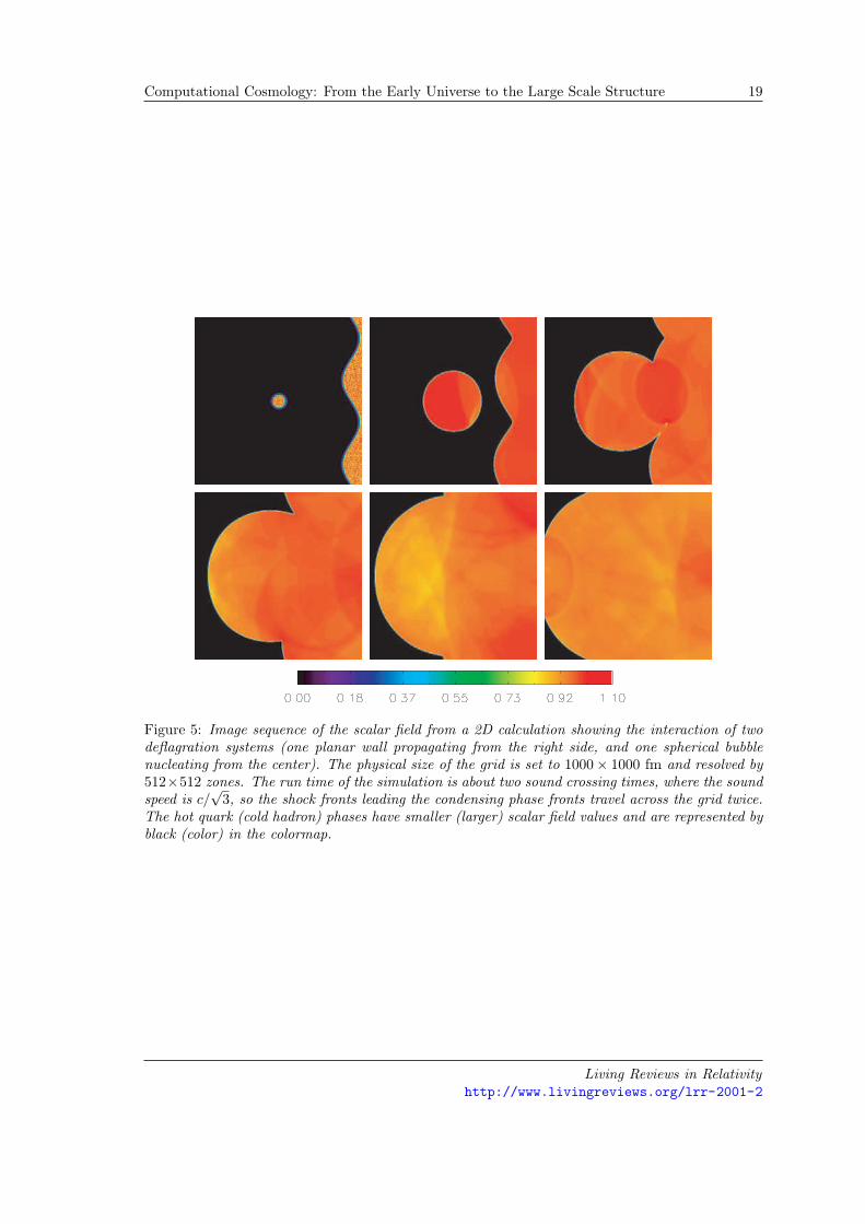
Fragile and Anninos [76] performed two-dimensional simulations of first order QCD transitionsto explore the nature of interface boundaries beyond linear stability analysis, and determine if they




Figure 5: Image sequence of the scalar field from a 2D calculation showing the interaction of twodeflagration systems (one planar wall propagating from the right side, and one spherical bubblenucleating from the center). The physical size of the grid is set to 1000× 1000 fm and resolved by512×512 zones. The run time of the simulation is about two sound crossing times, where the soundspeed is c/

√3, so the shock fronts leading the condensing phase fronts travel across the grid twice.

The hot quark (cold hadron) phases have smaller (larger) scalar field values and are represented byblack (color) in the colormap.



20 Peter Anninos

Figure 6: Image sequence of the scalar field from a 2D calculation showing the interaction of twodetonation systems (one planar wall propagating from the right side, and one spherical bubblenucleating from the center). The physical size of the grid is set to 1000× 1000 fm and resolved by1024× 1024 zones. The run time of the simulation is about two sound crossing times.




Figure 7: Image sequence of the scalar field from a 2D calculation showing the interaction of shockand rarefaction waves with a deflagration wall (initiated at the left side) and a detonation wall(starting from the right). A shock and rarefaction wave travel to the right and left, respectively,from the temperature discontinuity located initially at the grid center (the right half of the grid isat a higher temperature). The physical size of the domain is set to 1806.1×451.53 fm and resolvedby 2048× 512 zones. The run time of the simulation is about two sound crossing times.



22 Peter Anninos

are stable when the full nonlinearities of the relativistic scalar field and hydrodynamic system ofequations are accounted for. They used results from linear perturbation theory to define initialfluctuations on either side of the phase fronts and evolved the data numerically in time for bothdeflagration and detonation configurations. No evidence of mixing instabilities or hydrodynamicturbulence was found in any of the cases they considered, despite the fact that they investigated theparameter space predicted to be potentially unstable according to linear analysis. They also inves-tigated whether phase mixing can occur through a turbulence-type mechanism triggered by shockproximity or disruption of phase fronts. They considered three basic cases (see image sequences inFigures 5, 6, and 7 below): interactions between planar and spherical deflagration bubbles, colli-sions between planar and spherical detonation bubbles, and a third case simulating the interactionbetween both deflagration and detonation systems initially at two different thermal states. Theirresults are consistent with the standard picture of cosmological phase transitions in which hadronbubbles expand as spherical condensation fronts, undergoing regular (non-turbulent) coalescence,and eventually leading to collapsing spherical quark droplets in a medium of hadrons. This isgenerally true even in the detonation cases which are complicated by greater entropy heating fromshock interactions contributing to the irregular destruction of hadrons and the creation of quarknuggets.

However, Fragile and Anninos also note a deflagration ‘instability’ or acceleration mechanismevident in their third case for which they assume an initial thermal discontinuity in space separatingdifferent regions of nucleating hadron bubbles. The passage of a rarefaction wave (generated at thethermal discontinuity) through a slowly propagating deflagration can significantly accelerate thecondensation process, suggesting that the dominant modes of condensation in an early Universewhich super-cools at different rates within causally connected domains may be through super-sonic detonations or fast moving (nearly sonic) deflagrations. A similar speculation was made byKamionkowski and Freese [102] who suggested that deflagrations become unstable to perturbationsand are converted to detonations by turbulent surface distortion effects. However, in the simu-lations, deflagrations are accelerated not from turbulent mixing and surface distortion, but fromenhanced super-cooling by rarefaction waves. In multi-dimensions, the acceleration mechanism canbe exaggerated further by upwind phase mergers due to transverse flow, surface distortion, andmode dissipation effects, a combination that may result in supersonic front propagation speeds,even if the nucleation process began as a slowly propagating deflagration.

3.5 Nucleosynthesis

Observations of the light elements produced during Big Bang nucleosynthesis following the quark/hadron phase transition (roughly 10−2 – 102 s after the Big Bang) are in good agreement with thestandard model of our Universe (see Section 2.2). However, it is interesting to investigate othermore general models to assert the role of shear and curvature on the nucleosynthesis process, andplace limits on deviations from the standard model.

Rothman and Matzner [140] considered primordial nucleosynthesis in anisotropic cosmologies,solving the strong reaction equations leading to 4He. They find that the concentration of 4Heincreases with increasing shear due to time scale effects and the competition between dissipationand enhanced reaction rates from photon heating and neutrino blue shifts. Their results have beenused to place a limit on anisotropy at the epoch of nucleosynthesis. Kurki-Suonio and Matzner [109]extended this work to include 30 strong 2-particle reactions involving nuclei with mass numbersA ≤ 7, and to demonstrate the effects of anisotropy on the cosmologically significant isotopes 2H,3He, 4He and 7Li as a function of the baryon to photon ratio. They conclude that the effect ofanisotropy on 2H and 3He is not significant, and the abundances of 4He and 7Li increase withanisotropy in accord with [140].

Furthermore, it is possible that neutron diffusion, the process whereby neutrons diffuse out from




regions of very high baryon density just before nucleosynthesis, can affect the neutron to protonratio in such a way as to enhance deuterium and reduce 4He compared to a homogeneous model.However, plane symmetric, general relativistic simulations with neutron diffusion [110] show thatthe neutrons diffuse back into the high density regions once nucleosynthesis begins there – therebywiping out the effect. As a result, although inhomogeneities influence the element abundances,they do so at a much smaller degree then previously speculated. The numerical simulations alsodemonstrate that, because of the back diffusion, a cosmological model with a critical baryon densitycannot be made consistent with helium and deuterium observations, even with substantial baryoninhomogeneities and the anticipated neutron diffusion effect.

3.6 Cosmological gravitational waves

Gravitational waves are an inevitable product of the Einstein equations, and one can expect awide spectrum of wave signals propagating throughout our Universe due to anisotropic and inho-mogeneous metric and matter fluctuations, collapsing matter structures, ringing black holes, andcolliding neutron stars, for example. The discussion here is restricted to the pure vacuum fielddynamics and the fundamental nonlinear behavior of gravitational waves in numerically generatedcosmological spacetimes.

3.6.1 Planar symmetry

Centrella and Matzner [57, 58] studied a class of plane symmetric cosmologies representing gravi-tational inhomogeneities in the form of shocks or discontinuities separating two vacuum expandingKasner cosmologies (2). By a suitable choice of parameters, the constraint equations can be satis-fied at the initial time with a Euclidean 3-surface and an algebraic matching of parameters acrossthe different Kasner regions that gives rise to a discontinuous extrinsic curvature tensor. Theyperformed both numerical calculations and analytical estimates using a Green’s function analysisto establish and verify (despite the numerical difficulties in evolving discontinuous data) certainaspects of the solutions, including gravitational wave interactions, the formation of tails, and thesingularity behavior of colliding waves in expanding vacuum cosmologies.

Shortly thereafter, Centrella and Wilson [59, 60] developed a polarized plane symmetric code forcosmology, adding also hydrodynamic sources with artificial viscosity methods for shock capturingand Barton’s method for monotonic transport [162]. The evolutions are fully constrained (solvingboth the momentum and Hamiltonian constraints at each time step) and use the mean curvatureslicing condition. This work was subsequently extended by Anninos et al. [9, 11, 7], implementingmore robust numerical methods, an improved parametric treatment of the initial value problem,and generic unpolarized metrics.

In applications of these codes, Centrella [61] investigated nonlinear gravitational waves inMinkowski space and compared the full numerical solutions against a first order perturbationsolution to benchmark certain numerical issues such as numerical damping and dispersion. Asecond order perturbation analysis was used to model the transition into the nonlinear regime.Anninos et al. [10] considered small and large perturbations in the two degenerate Kasner models:p1 = p3 = 0 or 2/3, and p2 = 1 or −1/3, respectively, where pi are parameters in the Kasner met-ric (2). Carrying out a second order perturbation expansion and computing the Newman–Penrose(NP) scalars, Riemann invariants and Bel–Robinson vector, they demonstrated, for their particularclass of spacetimes, that the nonlinear behavior is in the Coulomb (or background) part representedby the leading order term in the NP scalar Ψ2, and not in the gravitational wave component. Forstanding-wave perturbations, the dominant second order effects in their variables are an enhancedmonotonic increase in the background expansion rate, and the generation of oscillatory behavior inthe background spacetime with frequencies equal to the harmonics of the first order standing-wavesolution.



24 Peter Anninos

Expanding these investigations of the Coulomb nonlinearity, Anninos and McKinney [16] useda gauge invariant perturbation formalism to construct constrained initial data for general relativis-tic cosmological sheets formed from the gravitational collapse of an ideal gas in a critically closedFLRW “background” model. They compared results to the Newtonian Zel’dovich [165] solutionover a broad range of field strengths and flows, and showed that the enhanced growth rates ofnonlinear modes (in both the gas density and Riemann curvature invariants) accelerate the col-lapse process significantly compared to Newtonian and perturbation theory. They also computedthe back-reaction of these structures to the mean cosmological expansion rate and found only asmall effect, even for cases with long wavelengths and large amplitudes. These structures were de-termined to produce time-dependent gravitational potential signatures in the CMBR (essentiallyfully relativistic Rees–Sciama effects) comparable to, but still dominated by, the large scale Sachs–Wolfe anisotropies. This confirmed, and is consistent with, the assumptions built into Newtoniancalculations of this effect.

3.6.2 Multi-dimensional vacuum cosmologies

Two additional examples of general relativistic codes developed for the purpose of investigatingdynamical behaviors in non-flat, vacuum, cosmological topologies are attributed to Holcomb [91]and Ove [129]. Holcomb considered vacuum axisymmetric models to study the structure of GeneralRelativity and the properties of gravitational waves in non-asymptotically flat spacetimes. Thecode was based on the ADM 3 +1 formalism and used Kasner matching conditions at the outeredges of the mesh, mean curvature slicing, and a shift vector to enforce the isothermal gaugein order to simplify the metric and to put it in a form that resembles quasi-isotropic coordinates.However, a numerical instability was observed in cases where the mesh domain exceeded the horizonsize. This was attributed to the particular gauge chosen, which does not appear well-suited to theKasner metric as it results in super-luminal coordinate velocities beyond the horizon scale.

Ove developed an independent code based on the ADM formalism to study cosmic censorshipissues, including the nature of singular behavior allowed by the Einstein equations, the role ofsymmetry in the creation of singularities, the stability of Cauchy horizons, and whether blackholes or a ring singularity can be formed by the collision of strong gravitational waves. Oveadopted periodic boundary conditions with 3-torus topology and a single Killing field, and thereforegeneralizes to two dimensions the planar codes discussed in the previous section. This code alsoused a variant of constant mean curvature slicing, was fully constrained at each time cycle, andthe shift vector was chosen to put the metric into a (time-dependent) conformally flat form at eachspatial hypersurface.




4 Physical Cosmology

The phrase “physical cosmology” is generally associated with the large (galaxy and cluster) scalestructure of the post-recombination epoch where gravitational effects are modeled approximately byNewtonian physics on an uniformly expanding, matter dominated FLRW background. A discussionof the large scale structure is included in this review since any viable model of our Universe whichallows a regime where strongly general relativistic effects are important must match onto theweakly relativistic (or Newtonian) regime. Also, since certain aspects of this regime are directlyobservable, one can hope to constrain or rule out various cosmological models and/or parameters,including the density (Ω0), Hubble (H0 = 100h km s−1 Mpc−1), and cosmological (Λ) constants.

Due to the vast body of literature on numerical simulations dealing with the post-recombinationepoch, only a very small fraction of published work can be reviewed in this paper. Hence, thefollowing summary is limited to cover just a few aspects of computational physical cosmology,and in particular those that can potentially be used to discriminate between cosmological modelparameters, even within the realm of the standard model.

For a general overview of theoretical and observational issues associated with structure forma-tion, the reader is referred to [132, 131], and to [45] for a broad review of numerical simulations(and methods) of structure formation.

4.1 Cosmic microwave background

The Cosmic Microwave Background Radiation (CMBR) is a direct relic of the early Universe, andcurrently provides the deepest probe of evolving cosmological structures. Although the CMBRis primarily a uniform black body spectrum throughout all space, fluctuations or anisotropies inthe spectrum can be observed at very small levels to correlate with the matter density distribu-tion. Comparisons between observations and simulations generally support the mostly isotropic,standard Big Bang model, and can be used to constrain the various proposed matter evolutionscenarios and cosmological parameters. For example, sky survey satellite observations [34, 149]suggest a flat Λ-dominated Universe with scale-invariant Gaussian fluctuations that is consistentwith numerical simulations of large sale structure formation (e.g., galaxy clusters, Lyα forest).

As shown in the timeline of Figure 8, CMBR signatures can be generally classified into twomain components: primary and secondary anisotropies, separated by a Surface of Last Scattering(SoLS). Both of these components include contributions from two distinctive phases: a surfacemarking the threshold of decoupling of ions and electrons from hydrogen atoms in primary signals,and a surface of reionization marking the start of multiphase secondary contributions throughnonlinear structure evolution, star formation, and radiative feedback from the small scales to thelarge.

4.1.1 Primordial black body effects

The black body spectrum of the isotropic background is essentially due to thermal equilibriumprior to the decoupling of ions and electrons, and few photon-matter interactions after that. Atsufficiently high temperatures, prior to the decoupling epoch, matter was completely ionized intofree protons, neutrons, and electrons. The CMB photons easily scatter off electrons, and frequentscattering produces a blackbody spectrum of photons through three main processes that occurfaster than the Universe expands:

• Compton scattering in which photons transfer their momentum and energy to electrons ifthey have significant energy in the electron’s rest frame. This is approximated by Thomsonscattering if the photon’s energy is much less than the rest mass. Inverse Compton scatteringis also possible in which sufficiently energetic (relativistic) electrons can blueshift photons.



26 Peter Anninos

Figure 8: Historical time-line of the cosmic microwave background radiation showing the start ofphoton/nuclei combination, the surface of last scattering (SoLS), and the epoch of reionizationdue to early star formation. The times are represented in years (to the right) and redshift (tothe left). Primary anisotropies are collectively attributed to the early effects at the last scatteringsurface and the large scale Sachs–Wolfe effect. Secondary anisotropies arise from path integrationeffects, reionization smearing, and higher order interactions with the evolving nonlinear structuresat relatively low redshifts.




• Double Compton scattering can both produce and absorb photons, and thus is able to ther-malize photons to a Planck spectrum (unlike Compton scattering which conserves photonnumber, and, although it preserves a Planck spectrum, relaxes to a Bose–Einstein distribu-tion).

• Bremsstrahlung emission of electromagnetic radiation due to the acceleration of electrons inthe vicinity of ions. This also occurs in reverse (free-free absorption) since charged particlescan absorb photons. In contrast to Coulomb scattering, which maintains thermal equilibriumamong baryons without affecting photons, Bremsstrahlung tends to relax photons to a Planckdistribution.

Although the CMBR is a unique and deep probe of both the thermal history of the earlyUniverse and primordial perturbations in the matter distribution, the associated anisotropies arenot exclusively primordial in nature. Important modifications to the CMBR spectrum, from bothprimary and secondary components, can arise from large scale coherent structures, even well afterthe photons decouple from the matter at redshift z ∼ 103, due to gravitational redshifting, lensing,and scattering effects.

4.1.2 Primary anisotropies

The most important contributions to primary anisotropies between the start of decoupling and thesurface of last scattering include the following effects:

• Sachs–Wolfe (SW) effect: Gravitational redshift of photons between potentials at the SoLSand the present. It is the dominant effect at large angular scales comparable to the horizonsize at decoupling (θ ∼ 2 Ω1/2).

• Doppler effect: Dipolar patterns are imprinted in the energy distribution from the peculiarvelocities of the matter structures acting as the last scatterers of the photons.

• Acoustic peaks: Anisotropies at intermediate angular scales (0.1 < θ < 2) are atttributed tosmall scale processes occurring until decoupling, including acoustic oscillations of the baryon-photon fluid from primordial density inhomogeneities. This gives rise to acoustic peaks inthe thermal spectrum representing the sound horizon scale at decoupling.

• SoLS damping: The electron capture rate is only slightly faster than photodissociation atthe start of decoupling, causing the SoLS to have a finite thickness (∆z ∼ 100). Scatteringover this interval damps fluctuations on scales smaller than the SoLS depth (θ < 10′ Ω1/2).

• Silk damping: Photons can diffuse out of overdense regions, dragging baryons with them oversmall angular scales. This tends to suppress both density and radiation fluctuations.

All of these mechanisms perturb the black body background radiation since thermalization pro-cesses are not efficient at redshifts smaller than ∼ 107.

4.1.3 Secondary anisotropies

Secondary anisotropies consist of two principal effects, gravitational and scattering. Some of themore important gravitational contributions to the CMB include:

• Early ISW effect: Photon contributions to the energy density of the Universe may be non-negligible compared to ordinary matter (dark or baryonic) at the last scattering. The de-creasing contribution of photons in time results in a decay of the potential, producing theearly Integrated Sachs–Wolfe (ISW) effect.



28 Peter Anninos

• Late ISW effect: In open cosmological models or models with a cosmological constant, thegravitational potential decays at late times due to a greater rate of expansion compared toflat spacetimes, producing the late ISW effect on large angular scales.

• Rees–Sciama effect: Evolving nonlinear strucutures (e.g., galaxies and clusters) generatetime-varying potentials which can seed asymmetric energy shifts in photons crossing potentialwells from the SoLS to the present.

• Lensing: In contrast to ISW effects which change the energy but not directions of the photons,gravitational lensing deflects the paths without changing the energy. This effectively smearsout the imaging of the SoLS.

• Proper motion: Compact objects such as galaxy clusters can imprint a dipolar pattern in theCMB as they move across the sky.

• Gravitational waves: Perturbations in the spacetime fabric affect photon paths, energies, andpolarizations, predominantly at scales larger than the horizon at decoupling.

Secondary scattering effects are associated with reionization and their significance depends onwhen and over what scales it takes place. Early reionization leads to large optical depths andgreater damping due to secondary scattering. Over large scales, reionization has little effect sincethese scales are not in causal contact. At small scales, primordial anisotropies can be wiped outentirely and replaced by secondary ones. Some of the more important secondary scattering effectsinclude:

• Thomson scattering: Photons are scattered by free electrons at sufficiently large opticaldepths achieved when the Universe undergoes a global reionization at late times. This dampsout fluctuations since energies are averaged over different directions in space.

• Vishniac effect: In a reionized Universe, high order coupling between the bulk flow of electronsand their density fluctuations generates new anisotropies at small angles.

• Thermal Sunyaev–Zel’dovich effect: Inverse Compton scattering of the CMB by hot electronsin the intracluster gas of a cluster of galaxies distorts the black body spectrum of the CMB.Low frequency photons will be shifted to high frequencies.

• Kinetic Sunyaev–Zel’dovich effect: The peculiar velocities of clusters produces anisotropiesvia a Doppler effect to shift the temperature without distorting the spectral form. Its effectis proportional to the product of velocity and optical depth.

• Polarization: Scattering of anisotropic radiation affects polarization due to the angular de-pendence of scattering. Polarization in turn affects anisotropies through a similar dependencyand tends to damp anisotropies.

To make meaningful comparisons between numerical models and observed data, all of these(low and high order) effects from both the primary and secondary contributions (see for exampleSection 4.1.4 and [94, 101]) must be incorporated self-consistently into any numerical model, and tohigh accuracy in order to resolve and distinguish amongst the various weak signals. The followingsections describe some work focused on incorporating many of these effects into a variety of large-scale numerical cosmological models.




4.1.4 Computing CMBR anisotropies with ray-tracing methods

Many efforts based on linear perturbation theory have been carried out to estimate temperatureanisotropies in our Universe (for example see [114] and references cited in [131, 94]). Althoughsuch linearized approaches yield reasonable results, they are not well-suited to discussing theexpected imaging of the developing nonlinear structures in the microwave background. Also,because photons are intrinsically coupled to the baryon and dark matter thermal and gravitationalstates at all spatial scales, a fully self-consistent treatment is needed to accurately resolve the moresubtle features of the CMBR. This can be achieved with a ray-tracing approach based on Monte-Carlo methods to track individual photons and their interactions through the evolving matterdistributions. A fairly complete simulation involves solving the geodesic equations of motion forthe collisionless dark matter which dominate potential interactions, the hydrodynamic equationsfor baryonic matter with high Mach number shock capturing capability, the transport equations forphoton trajectories, a reionization model to reheat the Universe at late times, the chemical kineticsequations for the ion and electron concentrations of the dominant hydrogen and helium gases,and the photon-matter interaction terms describing scattering, redshifting, depletion, lensing, andDoppler effects.

Such an approach has been developed by Anninos et al. [15], and applied to a Hot Dark Matter(HDM) model of structure formation. In order to match both the observed galaxy-galaxy corre-lation function and COBE measurements of the CMBR, they find, for that model and neglectingreionization, the cosmological parameters are severely constrained to Ω0h

2 ≈ 1, where Ω0 and hare the density and Hubble parameters respectively.

In models where the IGM does not reionize, the probability of scattering after the photon-matter decoupling epoch is low, and the Sachs–Wolfe effect dominates the anisotropies at angularscales larger than a few degrees. However, if reionization occurs, the scattering probability increasessubstantially and the matter structures, which develop large bulk motions relative to the comovingbackground, induce Doppler shifts on the scattered CMBR photons and leave an imprint of thesurface of last scattering. The induced fluctuations on subhorizon scales in reionization scenarioscan be a significant fraction of the primordial anisotropies, as observed by Tuluie et al. [157] alsousing ray-tracing methods. They considered two possible scenarios of reionization: A model thatsuffers early and gradual (EG) reionization of the IGM as caused by the photoionizing UV radiationemitted by decaying neutrinos, and the late and sudden (LS) scenario as might be applicable to thecase of an early generation of star formation activity at high redshifts. Considering the HDM modelwith Ω0 = 1 and h = 0.55, which produces CMBR anisotropies above current COBE limits whenno reionization is included (see Section 4.1.4), they find that the EG scenario effectively reducesthe anisotropies to the levels observed by COBE and generates smaller Doppler shift anisotropiesthan the LS model, as demonstrated in Figure 9. The LS scenario of reionization is not able toreduce the anisotropy levels below the COBE limits, and can even give rise to greater Dopplershifts than expected at decoupling.

Additional sources of CMBR anisotropy can arise from the interactions of photons with dy-namically evolving matter structures and nonstatic gravitational potentials. Tuluie et al. [156]considered the impact of nonlinear matter condensations on the CMBR in Ω0 ≤ 1 Cold DarkMatter (CDM) models, focusing on the relative importance of secondary temperature anisotropiesdue to three different effects: (i) time-dependent variations in the gravitational potential of non-linear structures as a result of collapse or expansion (the Rees–Sciama effect), (ii) proper motionof nonlinear structures such as clusters and superclusters across the sky, and (iii) the decayinggravitational potential effect from the evolution of perturbations in open models. They appliedthe ray-tracing procedure of [15] to explore the relative importance of these secondary anisotropiesas a function of the density parameter Ω0 and the scale of matter distributions. They find thatsecondary temperature anisotropies are dominated by the decaying potential effect at large scales,



30 Peter Anninos

Figure 9: Temperature fluctuations (∆T/T ) in the CMBR due to the primary Sachs–Wolfe (SW)effect and secondary integrated SW, Doppler, and Thomson scattering effects in a critically closedmodel. The top two plates are results with no reionization and baryon fractions 0.02 (plate 1, 4o×4o,∆T/T |rms = 2.8×10−5), and 0.2 (plate 2, 8×8, ∆T/T |rms = 3.4×10−5). The bottom two platesare results from an ”early and gradual” reionization scenario of decaying neutrinos with baryonfraction 0.02 (plate 3, 4×4, ∆T/T |rms = 1.3×10−5; and plate 4, 8×8, ∆T/T |rms = 1.4×10−5).If reionization occurs, the scattering probability increases and anisotropies are damped with eachscattering event. At the same time, matter structures develop large bulk motions relative to thecomoving background and induce Doppler shifts on the CMB. The imprint of this effect from lastscattering can be a significant fraction of primary anisotropies.




but that all three sources of anisotropy can produce signatures of order ∆T/T |rms ∼ 10−6 as shownin Figure 10.

In addition to the effects discussed in this section, many other sources of secondary anisotropies(as mentioned in Section 4.1, including gravitational lensing, the Vishniac effect accounting for mat-ter velocities and flows into local potential wells, and the Sunyaev–Zel’dovich (SZ) (Section 4.5.4)distortions from the Compton scattering of CMB photons by electrons in the hot cluster medium)can also be fairly significant. See [94, 152, 28, 80, 93] for more thorough discussions of the differentsources of CMBR anisotropies.

4.2 Gravitational lensing

Observations of gravitational lenses [143] provide measures of the abundance and strength of non-linear potential fluctuations along the lines of sight to distant objects. Since these calculations aresensitive to the gravitational potential, they may be more reliable than galaxy and velocity fieldmeasurements as they are not subject to the same ambiguities associated with biasing effects. Also,because different cosmological models predict different mass distributions, especially at the higherredshifts, lensing calculations can potentially be used to confirm or discard competing cosmologicalmodels.

As an alternative to solving the computationally demanding lens equations, Cen et al. [55] de-veloped an efficient scheme to identify regions with surface densities capable of generating multipleimages accurately for splittings larger than three arcseconds. They applied this technique to astandard CDM model with Ω0 = 1, and found that this model predicts more large angle splittings(> 8′′) than are known to exist in the observed Universe. Their results suggest that the standardCDM model should be excluded as a viable model of our Universe. A similar analysis for a flatlow density CDM model with a cosmological constant (Ω0 = 0.3, Λ/3H2

0 = 0.7) suggests a lowerand perhaps acceptable number of lensing events. However, an uncertainty in their studies is thenature of the lenses at and below the resolution of the numerical grid. They model the lensingstructures as simplified Singular Isothermal Spheres (SIS) with no distinctive cores.

Large angle splittings are generally attributed to larger structures such as clusters of galaxies,and there are indications that clusters have small but finite core radii rcore ∼ 20 – 30h−1 kpc.Core radii of this size can have an important effect on the probability of multiple imaging. Flo-res and Primack [74] considered the effects of assuming two different kinds of splitting sources:isothermal spheres with small but finite core radii and radial density profiles ρ ∝ (r2 + r2core)

−1,and spheres with a Hernquist density profile ρ ∝ r−1(r + a)−3, where rcore ∼ 20 – 30h−1 kpc anda ∼ 300h−1 kpc. They find that the computed frequency of large-angle splittings, when using thenonsingular profiles, can potentially decrease by more than an order of magnitude relative to theSIS case and can bring the standard CDM model into better agreement with observations. Theystress that lensing events are sensitive to both the cosmological model (essentially the numberdensity of lenses) and to the inner lens structure, making it difficult to probe the models until thestructure of the lenses, both observationally and numerically, is better known.

4.3 First star formation

In CDM cosmogonies, the fluctuation spectrum at small wavelengths has a logarithmic dependenceat mass scales smaller than 108 solar masses, which indicates that all small scale fluctuations inthis model collapse nearly simultaneously in time. This leads to very complex dynamics duringthe formation of these first structures. Furthermore, the cooling in these fluctuations is dominatedby the rotational/vibrational modes of hydrogen molecules that were able to form using the freeelectrons left over from recombination and those produced by strong shock waves as catalysts.The first structures to collapse may be capable of producing pop III stars and have a substantial



32 Peter Anninos

Figure 10: Secondary anisotropies from the proper motion of galaxy clusters across the sky andRees–Sciama effects are presented in the upper-left image over 8 × 8 in a critically closed ColdDark Matter model. The corresponding column density of matter over the same region (z = 0.43,∆z = 0.025) is displayed in the upper-right, clearly showing the dipolar nature of the proper mo-tion effect. Anisotropies arising from decaying potentials in an open Ω = 0.3 model over a scaleof 8 × 8 are shown in the bottom left image, along with the gravitational potential over the sameregion (z = 0.33, ∆z = 0.03) in the bottom right, demonstrating a clear anti-correlation. Maxi-mum temperature fluctuations in each simulation are ∆T/T = (5× 10−7, 1.0× 10−6) respectvely.Secondary anisotropies are dominated by decaying potentials at large scales, but all three sources(decaying potential, proper motion, and R-S) produce signatures of order 10−6.




influence on the subsequent thermal evolution of the intergalactic medium, as suggested by Figure 2,due to the radiation emitted by the first generation stars as well as supernova driven winds. Toknow the subsequent fate of the Universe and which structures will survive or be destroyed by theUV background, it is first necessary to know when and how the first stars formed.

Ostriker and Gnedin [127] have carried out high resolution numerical simulations of the reheat-ing and reionization of the Universe due to star formation bursts triggered by molecular hydrogencooling. Accounting for the chemistry of the primeval hydrogen/helium plasma, self-shielding ofthe gas, radiative cooling, and a phenomenological model of star formation, they find that twodistinct star populations form: the first generation pop III from H2 cooling prior to reheating atredshift z ≥ 14; and the second generation pop II at z < 10 when the virial temperature of thegas clumps reaches 104 K and hydrogen line cooling becomes efficient. Star formation slows in theintermittent epoch due to the depletion of H2 by photo-destruction and reheating. In addition, theobjects which formed pop III stars also initiate pop II sequences when their virial temperaturesreach 104 K through continued mass accretion.

In resolving the details of a single star forming region in a CDM Universe, Abel et al. [2, 3]implemented a non-equilibrium radiative cooling and chemistry model [1, 21] together with thehydrodynamics and dark matter equations, evolving nine separate atomic and molecular species(H, H+, He, He+, He++, H−, H+

2 , H2, and e−, according to the reactive network described inSection 6.4.1) on nested and adaptively refined numerical grids. They follow the collapse andfragmentation of primordial clouds over many decades in mass and spatial dynamical range, findinga core of mass ∼ 200M forms from a halo of about ∼ 105M (where a significant number fractionof hydrogen molecules are created) after less than one percent of the halo gas cools by molecularline emission. Bromm et al. [48] use a different Smoothed Particle Hydrodynamics (SPH) techniqueand a six species model (H, H+, H−, H+

2 , H2, and e−) to investigate the initial mass function ofthe first generation pop III stars. They evolve an isolated 3σ peak of mass 2 × 106M whichcollapses at redshift z ∼ 30 and forms clumps of mass 102 – 103M which then grow by accretionand merging, suggesting that the very first stars were massive and in agreement with [3].

The implications of an early era of massive star populations on the thermal and chemical stateof the intergalactic medium was investigated by Yoshida et al. [164]. They considered the effects offeedback and radiation transfer in early structure formation simulations to show that a significantfraction of the IGM can be ionized and polluted by metals from the first stars to form and becomesupernovae by z ∼ 15, thus affecting subsequent stellar populations. They also argue that observedelemental abundances in the intracluster medium are not affected by metals originating from thefirst stars.

4.4 Lyα forest

The Lyα forest represents the optically thin (at the Lyman edge) component of Quasar AbsorptionSystems (QAS), a collection of absorption features in quasar spectra extending back to high red-shifts. QAS are effective probes of the matter distribution and the physical state of the Universeat early epochs when structures such as galaxies are still forming and evolving. The relative lack ofconstraining observational data at the intermediate to high redshifts (0 < z < 5), where differencesbetween competing cosmological models are more pronounced, suggests that QAS can potentiallyyield valuable and discriminating observational data.

Many complex multi-component numerical simulations have been performed of the Lymanforest, which include the effects of dark matter (N-body), baryons (hydrodynamics), chemicalcomposition (reactive networks), and microphysical response (radiative cooling and heating). See,for example, [67, 118, 166], which represent some of the earliest comprehensive simulations. For themost part, all these calculations have been able to fit the observations reasonably well, including thecolumn density and Doppler width distributions, the size of absorbers [62], and the line number



34 Peter Anninos

evolution. Despite the fact that the cosmological models and parameters are different in eachcase, the simulations give roughly similar results provided that the proper ionization bias is used,bion ≡ (Ωbh

2)2/Γ, where Ωb is the baryonic density parameter, h is the Hubble parameter andΓ is the photoionization rate at the hydrogen Lyman edge. (However, see [50] for a discussion ofthe sensitivity of statistical properties on numerical resolution.) A theoretical paradigm has thusemerged from these calculations in which Lyα absorption lines originate from the relatively smallerscale structure in pregalactic or intergalactic gas through the bottom-up hierarchical formationpicture in CDM-like Universes. The absorption features originate in structures exhibiting a varietyof morphologies commonly found in numerical simulations (see Figure 11), including fluctuationsin underdense regions, spheroidal minihalos, and filaments extending over scales of a few Mpc.

Machacek et al. [115] expanded on earlier work to compare several Lyα statistical measuresfrom five different background cosmological models, including standard critical density Cold DarkMatter (CDM), open CDM, flat CDM with a cosmological constant, standard CDM with a tilteddensity spectrum, and a flat model with mixed hot and cold dark matter. All models were chosen tomatch local or low redshift observations, and most were also consistent with COBE measurementsof the CMBR. The calculations were designed to establish which statistics are sensitive to differentcosmological models. In particular, they find that the line number count above a given columndensity threshold is relatively insensitive to background models. On the other hand, the shape ofthe optical depth probability distribution function is strongly correlated to the amount of smallscale power in density fluctuations, and is thus a good discriminator among models on scales of afew hundred kpc.

Meiksin et al. [117] followed up with more detailed comparisons of Lyα systems in severalcosmologies with observed high resolution QSO spectra. Although all models are consistent withprevious studies in that they give reasonably good statistical agreement with observed Lyα proper-ties, under closer scrutiny none of the numerical models they considered passed all the tests, whichincluded spectral flux, wavelet decomposed amplitude, and absorption line profile distributions.They suggest that comparisons might be improved, particularly in optically thin systems, by moreenergy injection into the IGM from late He+ reionization or supernovae-driven winds, or by alarger baryon fraction.

4.5 Galaxy clusters

Clusters of galaxies are the largest gravitationally bound systems known to be in quasi-equilibrium.This allows for reliable estimates to be made of their mass as well as their dynamical and ther-mal attributes. The richest clusters, arising from 3σ density fluctuations, can be as massive as1014 – 1015M, and the environment in these structures is composed of shock heated gas withtemperatures of order 107mbox−− 108 K which emits thermal bremsstrahlung and line radiationat X-ray energies. Also, because of their spatial size of ∼ 1h−1 Mpc and separations of order50h−1 Mpc, they provide a measure of nonlinearity on scales close to the perturbation normal-ization scale 8h−1 Mpc. Observations of the substructure, distribution, luminosity, and evolutionof galaxy clusters are therefore likely to provide signatures of the underlying cosmology of ourUniverse, and can be used as cosmological probes in the observable redshift range 0 ≤ z ≤ 1.

4.5.1 Internal structure

Thomas et al. [155] investigated the internal structure of galaxy clusters formed in high resolutionN-body simulations of four different cosmological models, including standard, open, and flat butlow density Universes. They find that the structure of relaxed clusters is similar in the criticaland low density Universes, although the critical density models contain relatively more disorderedclusters due to the freeze-out of fluctuations in open Universes at late times. The profiles of relaxed




Figure 11: Distribution of the gas density at redshift z = 3 from a numerical hydrodynamicssimulation of the Lyα forest with a CDM spectrum normalized to second year COBE observations,Hubble parameter of h = 0.5, a comoving box size of 9.6 Mpc, and baryonic density of Ωb = 0.06composed of 76% hydrogen and 24% helium. The region shown is 2.4 Mpc (proper) on a side.The isosurfaces represent baryons at ten times the mean density and are color coded to the gastemperature (dark blue = 3×104 K, light blue = 3×105 K). The higher density contours trace outisolated spherical structures typically found at the intersections of the filaments. A single randomslice through the cube is also shown, with the baryonic overdensity represented by a rainbow-likecolor map changing from black (minimum) to red (maximum). The He+ mass fraction is shownwith a wire mesh in this same slice. To emphasize fine structure in the minivoids, the mass fractionin the overdense regions has been rescaled by the gas overdensity wherever it exceeds unity.



36 Peter Anninos

clusters are very similar in the different simulations since most clusters are in a quasi-equilibriumstate inside the virial radius and generally follow the universal density profile of Navarro et al. [125].There does not appear to be a strong cosmological dependence in the profiles as suggested byprevious studies of clusters formed from pure power law initial density fluctuations [65]. However,because more young and dynamically evolving clusters are found in critical density Universes,Thomas et al. suggest that it may be possible to discriminate among the density parameters bylooking for multiple cores in the substructure of the dynamic cluster population. They note that astatistical population of 20 clusters could distinguish between open and critically closed Universes.

4.5.2 Number density evolution

The evolution of the number density of rich clusters of galaxies can be used to compute Ω0 and σ8

(the power spectrum normalization on scales of 8h−1 Mpc) when numerical simulation results arecombined with the constraint σ8Ω0.5

0 ≈ 0.5, derived from observed present-day abundances of richclusters. Bahcall et al. [24] computed the evolution of the cluster mass function in five differentcosmological model simulations and find that the number of high mass (Coma-like) clusters in flat,low σ8 models (i.e., the standard CDM model with σ8 ≈ 0.5) decreases dramatically by a factor ofapproximately 103 from z = 0 to z ≈ 0.5. For low Ω0, high σ8 models, the data result in a muchslower decrease in the number density of clusters over the same redshift interval. Comparing theseresults to observations of rich clusters in the real Universe, which indicate only a slight evolutionof cluster abundances to redshifts z ≈0.5–1, they conclude that critically closed standard CDMand Mixed Dark Matter (MDM) models are not consistent with the observed data. The modelswhich best fit the data are the open models with low bias (Ω0 = 0.3 ± 0.1 and σ8 = 0.85 ± 0.5),and flat low density models with a cosmological constant (Ω0 = 0.34± 0.13 and Ω0 + Λ = 1).

4.5.3 X-ray luminosity function

The evolution of the X-ray luminosity function, as well as the number, size and temperaturedistribution of galaxy clusters are all potentially important discriminants of cosmological modelsand the underlying initial density power spectrum that gives rise to these structures. Because the X-ray luminosity (principally due to thermal bremsstrahlung emission from electron/ion interactionsin the hot fully ionized cluster medium) is proportional to the square of the gas density, the contrastbetween cluster and background intensities is large enough to provide a window of observations thatis especially sensitive to cluster structure. Comparisons of simulated and observed X-ray functionsmay be used to deduce the amplitude and shape of the fluctuation spectrum, the mean densityof the Universe, the mass fraction of baryons, the structure formation model, and the backgroundcosmological model.

Several groups [49, 56] have examined the properties of X-ray clusters in high resolution nu-merical simulations of a standard CDM model normalized to COBE. Although the results are verysensitive to grid resolution (see [17] for a discussion of the effects from resolution constraints on theproperties of rich clusters), their primary conclusion, that the standard CDM model predicts toomany bright X-ray emitting clusters and too much integrated X-ray intensity, is robust since anincrease in resolution will only exaggerate these problems. On the other hand, similar calculationswith different cosmological models [56, 52] suggest reasonable agreement of observed data withCold Dark Matter + cosmological constant (ΛCDM), Cold + Hot Dark Matter (CHDM), andOpen or low density CDM (OCDM) evolutions due to different universal expansions and densitypower spectra.




4.5.4 SZ effect

The Sunyaev–Zel’dovich (SZ) effect is the change in energy that CMB photons undergo when theyscatter in hot gas typically found in cores of galaxy clusters. There are two main effects: thermaland kinetic. Thermal SZ is the dominant mechanism which arises from thermal motion of gas inthe temperature range 107 – 108 K, and is described by the Compton y parameter

y = σT

∫nekBTe

mec2dl, (7)

where σT = 6.65×10−25 cm2 is the Thomson cross-section, me, ne and Te are the electron rest mass,density and temperature, c is the speed of light, kB is Boltzmann’s constant, and the integration isperformed over the photon path. Photon temperature anisotropies are related to the y parameterby ∆T/T ≈ −2y in the Rayleigh–Jeans limit. The kinetic SZ effect is a less influential Dopplershift resulting from the bulk motion of ionized gas relative to the rest frame of the CMB.

Springel et al. [150] used a Tree/SPH code to study the SZ effects in a CDM cosmology witha cosmological constant. They find a mean amplitude for thermal SZ (y = 3.8× 10−6) just belowcurrent observed upper limits, and a kinetic SZ about 30 times smaller in power. Da Silva et al. [66]compared thermal SZ maps in three different cosmologies (low density + Λ, critical density, andlow density open model). Their results are also below current limits: y ≈ 4× 10−6 for low densitymodels with contributions from over a broad redshift range z ≤ 5, and y ≈ 1×10−6 for the criticaldensity model with contributions mostly from z < 1. However, further simulations are needed toexplore the dependence of the SZ effect on microphysics, i.e., cooling, star formation, supernovaefeedback.

4.6 Cosmological sheets

Cosmological sheets, or pancakes, form as overdense regions collapse preferentially along one axis.Originally studied by Zel’dovich [165] in the context of neutrino-dominated cosmologies, sheets areubiquitous features in nonlinear structure formation simulations of CDM-like models with baryonicfluid, and manifest on a spectrum of length scales and formation epochs. Gas collapses gravita-tionally into flattened sheet structures, forming two plane parallel shock fronts that propagate inopposite directions, heating the infalling gas. The heated gas between the shocks then cools radia-tively and condenses into galactic structures. Sheets are characterized by essentially five distinctcomponents: the preshock inflow, the postshock heated gas, the strongly cooling/recombinationfront separating the hot gas from the cold, the cooled postshocked gas, and the unshocked adiabati-cally compressed gas at the center. Several numerical calculations [47, 145, 22] have been performedof these systems which include baryonic fluid with hydrodynamical shock heating, ionization, re-combination, dark matter, thermal conductivity, and radiative cooling (Compton, bremsstrahlung,and atomic line cooling), in both one and two spatial dimensions to assert the significance of eachphysical process and to compute the fragmentation scale. See also [16] where fully general rela-tivistic numerical calculations of cosmological sheets are presented in plane symmetry, includingrelativistic hydrodynamical shock heating and consistent coupling to spacetime curvature.

In addition, it is well known that gas which cools to 1 eV through hydrogen line cooling willlikely cool faster than it can recombine. This nonequilibrium cooling increases the number ofelectrons and ions (compared to the equilibrium case) which, in turn, increases the concentrationsof H− and H+

2 , the intermediaries that produce hydrogen molecules H2. If large concentrationsof molecules form, excitations of the vibrational/rotational modes of the molecules can efficientlycool the gas to well below 1 eV, the minimum temperature expected from atomic hydrogen linecooling. Because the gas cools isobarically, the reduction in temperature results in an even greaterreduction in the Jeans mass, and the bound objects which form from the fragmentation of H2



38 Peter Anninos

cooled cosmological sheets may be associated with massive stars or star clusters. Anninos andNorman [18] have carried out 1D and 2D high resolution numerical calculations to investigatethe role of hydrogen molecules in the cooling instability and fragmentation of cosmological sheets,considering the collapse of perturbation wavelengths from 1 Mpc to 10 Mpc. They find thatfor the more energetic (long wavelength) cases, the mass fraction of hydrogen molecules reachesnH2/nH ∼ 3 × 10−3, which cools the gas to 4 × 10−3 eV and results in a fragmentation scale of9× 103M. This represents reductions of 50 and 103 in temperature and Jeans mass respectivelywhen compared, as in Figure 12, to the equivalent case in which hydrogen molecules were neglected.

However, the above calculations neglected important interactions arising from self-consistenttreatments of radiation fields with ionizing and photo-dissociating photons and self-shielding effects.Susa and Umemura [153] studied the thermal history and hydrodynamical collapse of pancakes ina UV background radiation field. They solve the radiative transfer of photons together withthe hydrodynamics and chemistry of atomic and molecular hydrogen species. Although theirsimulations were restricted to one-dimensional plane parallel symmetry, they suggest a classificationscheme distinguishing different dynamical behavior and galaxy formation scenarios based on theUV background radiation level and a critical mass corresponding to 1 − 2σ density fluctuationsin a standard CDM cosmology. These level parameters distinguish galaxy formation scenarios asthey determine the local thermodynamics, the rate of H2 line emissions and cooling, the amountof starburst activity, and the rate and mechanism of cloud collapse.

Figure 12: Two different model simulations of cosmological sheets are presented: a six species modelincluding only atomic line cooling (left), and a nine species model including also hydrogen molecules(right). The evolution sequences in the images show the baryonic overdensity and gas temperatureat three redshifts following the initial collapse at z = 5. In each figure, the vertical axis is 32 kpclong (parallel to the plane of collapse) and the horizontal axis extends to 4 Mpc on a logarithmicscale to emphasize the central structures. Differences in the two cases are observed in the coldpancake layer and the cooling flows between the shock front and the cold central layer. When thecentral layer fragments, the thickness of the cold gas layer in the six (nine) species case grows to3 (0.3) kpc and the surface density evolves with a dominant transverse mode corresponding to ascale of approximately 8 (1) kpc. Assuming a symmetric distribution of matter along the secondtransverse direction, the fragment masses are approximately 107 (105) solar masses.




5 Summary

This review is intended to provide a flavor of the variety of numerical cosmological calculationsperformed of different events occurring throughout the history of our Universe. The topics dis-cussed range from the strong field dynamical behavior of spacetime geometry at early times nearthe Big Bang singularity and the epoch of inflation, to the late time evolution of large scale matterfluctuations and the formation of clusters of galaxies. For the most part, the nature of the calcula-tions dealing with the early or late Universe can be distinguished by their basic motivations. Forexample, calculations of early Universe phenomena are designed to explore alternative cosmologicalmodels or topologies, and in some cases, different theories of gravity. They also tend to study thenature of topological singularities, geometric effects, and the problem of initial conditions or theorigin of matter distributions. Calculations of the late Universe are generally focused to establishbounds on cosmological parameters in the context of the standard model, to resolve the correctstructure formation scenario, to model the complex multi-physics interactions operating at vastlydifferent scales, and to systematically compare invariant measures against observed data for bothmodel validation and interpreting observations.

Although a complete, self-consistent, and accurate description of our Universe is impracticalconsidering the complex multi-scale and multi-physics requirements, a number of enlightening re-sults have been demonstrated through computations. For example, both monotonic AVTD andchaotic oscillatory BLK behavior have been found in the asymptotic approach to the initial singu-larity in a number of inhomogeneous cosmological models, though some issues remain concerningthe generic nature of the singularity, including the effect of nonlinear mode coupling of spatial gra-dients to the oscillatory history, and the behavior in non-vacuum spacetimes with arbitrary globaltopology. Numerical calculations suggest that scalar fields play an important complicated role inthe nonlinear or chaotic evolution of cosmological models with consequences for the triggering (ornot) of inflation and the subsequent dynamics of structure formation. It is possible, for example,that these fields can influence the details of inflation and have observable ramifications as fractalpatterns in the density spectrum, gravitational waves, galaxy distribution, and cosmic microwavebackground anisotropies. All these effects require further studies. Numerical simulations have alsobeen used to place limits on curvature anisotropies and cosmological parameters at early times byconsidering primordial nucleosynthesis reactions in anisotropic and inhomogeneous cosmologies.

Finally, the large collection of calculations performed of the post-recombination epoch related tolarge scale structure formation (for example, cosmic microwave background, gravitational lensing,Lyα absorption, and galaxy cluster simulations) have placed strong constraints on the standardmodel parameters and structure formation scenarios when compared to observations. Consideringthe range of models consistent with inflation, the preponderance of observational, theoretical andcomputational data suggest a best fit model of the late structure-forming Universe that is spatiallyflat with a cosmological constant and a small tilt in the power spectrum. These best fit modelparameters, and in particular the introduction of a cosmological constant, are generally consistentwith recent evidence of dark energy from supernovae and high precision CMBR observations.

Obviously many fundamental issues remain unresolved, including even the overall shape ortopology of the cosmological model which best describes our Universe throughout its entire history.However, the field of numerical cosmology has matured in the development of computationaltechniques, the modeling of microphysics, and in taking advantage of current trends in computingtechnologies, to the point that it is now possible to perform high resolution multiphysics simulationsand carry out reliable comparisons of numerical models with observational data.



40 Peter Anninos

6 Appendix: Basic Equations and Numerical Methods

Some basic equations relevant for fully relativistic as well as perturbative cosmological calculationsare summarized in this section, including the complete Einstein equations, choices of kinematicalconditions, initial data constraints, stress-energy-momentum tensors, dynamical equations for var-ious matter sources, and the Newtonian counterparts on background isotropic models. Referencesto numerical methods are also provided.

6.1 The Einstein equations

6.1.1 ADM formalism

There are many ways to write the Einstein equations. The most common is the ADM or 3+ 1form [23] which decomposes spacetime into layers of three-dimensional space-like hypersurfaces,threaded by a time-like normal congruence nµ = (1,−βi)/α, where we use Greek (Latin) indicesto specify spacetime (spatial) quantities. The general spacetime metric is written as

ds2 = (−α2 + βiβi) dt2 + 2βi dxi dt+ γij dx

i dxj , (8)

where α and βi are the lapse function and shift vector respectively, and γij is the spatial 3-metric.The lapse defines the proper time between consecutive layers of spatial hypersurfaces, the shiftpropagates the coordinate system from 3-surface to 3-surface, and the induced 3-metric is relatedto the 4-metric via γµν = gµν + nµnν . The Einstein equations are written as four constraintequations,

(3)R+K2 −KijKij = 16πGρH, (9)

∇i(Kij − γijK

)= 8πGsj , (10)

twelve evolution equations,

∂tγij = Lβγij − 2αKij ,

∂tKij = LβKij −∇i∇jα+ α

[(3)Rij − 2KikK

kj +KKij − 8πG

(sij −

12sγij +

12ρHγij

)],

(11)

and four kinematical or coordinate conditions for the lapse function and shift vector that can bespecified arbitrarily (see Section 6.1.2). Here Kij is the extrinsic curvature describing how the3-metric evolves along a time-like normal vector. It is formally defined as the Lie derivative (Ln)of the spatial metric along the vector nµ, Kij ≡ −Lnγij/2. Also,

Lβγij = ∇iβj +∇jβi,

LβKij = βk∇kKij +Kik∇jβk +Kkj∇iβk,(12)

where ∇i is the spatial covariant derivative with respect to γij , (3)Rij is the spatial Ricci tensor, Kis the trace of the extrinsic curvature Kij , and G is the gravitational constant. The matter sourceterms ρH, sj , sij and s = sii as seen by the observers at rest in the time slices are obtained fromthe appropriate projections

ρH = nµnνTµν , (13)si = −γµi n

νTµν , (14)sij = γµi γ

νj Tµν (15)

for the energy density, momentum density and spatial stresses, respectively. Here c = 1, and Greek(Latin) indices refer to 4(3)-dimensional quantities.




It is worth noting that several alternative formulations of Einstein’s equations have been sug-gested, including hyperbolic systems [136] which have nice mathematical properties, and conformaltraceless systems [147, 31] which make use of a conformal decomposition of the 3-metric and trace-free part of the extrinsic curvature Aij = Kij−γij K/3. Introducing γij = e−4ψγij with e4ψ = γ1/3

so that the determinant of γij is unity, and Aij = e−4ψAij , evolution equations can be written inthe conformal traceless system for ψ, γij , K, Aij and the conformal connection functions, thoughnot all of these variables are independent. However, it is not yet entirely clear which of thesemethods is best suited for generic problems. For example, hyperbolic forms are easier to charac-terize mathematically than ADM and may potentially be more stable, but can suffer from greaterinaccuracies by introducing additional equations or higher order derivatives. Conformal treatmentsare considered to be generally more stable [31], but can be less accurate than traditional ADM forshort term evolutions [6].

Many numerical methods have been used to solve the Einstein equations, including variantsof the leapfrog scheme, the method of McCormack, the two-step Lax–Wendroff method, and theiterative Crank–Nicholson scheme, among others. For a discussion and comparison of the differentmethods, the reader is referred to [43], where a systematic study was carried out on sphericallysymmetric black hole spacetimes using traditional ADM, and to [31, 6, 13] (and references therein)which discuss the stability and accuracy of hyperbolic and conformal treatments.

6.1.2 Kinematic conditions

For cosmological simulations, one typically takes the shift vector to be zero, hence Lβγij = LβKij =0. However, the shift can be used advantageously in deriving conditions to maintain the 3-metricin a particular form, and to simplify the resulting differential equations [59, 60]. See also [146]describing an approximate minimum distortion gauge condition used to help stabilize simulationsof general relativistic binary clusters and neutron stars.

Several options can be implemented for the lapse function, including geodesic (α = 1), algebraic,and mean curvature slicing. The algebraic condition takes the form

α = F1(xµ)F2(γ), (16)

where F1(xµ) is an arbitrary function of coordinates xµ, and F2(γ) is a dynamic function ofthe determinant of the 3-metric. This choice is computationally cheap, simple to implement,and certain choices of F2 (i.e., 1 + ln γ) can mimic maximal slicing in its singularity avoidanceproperties [8]. On the other hand, numerical solutions derived from harmonically-sliced foliationscan exhibit pathological gauge behavior in the form of coordinate “shocks” or singularities whichwill affect the accuracy, convergence and stability of solutions [5, 86]. Also, evolutions in which thelapse function is fixed by some analytically prescribed method (either geodesic or near-geodesic)can be unstable, especially for sub-horizon scale perturbations [7].

The mean curvature slicing equation is derived by taking the trace of the extrinsic curvatureevolution equation (11),

∇i∇iα = α[KijK

ij + 4πG (ρH + s)]+ βi∇iK − ∂tK, (17)

and assuming K = K(t), which can either be specified arbitrarily or determined by imposing aboundary condition on the lapse function after solving Equation (17) for the quantity α/∂tK [60].It is also useful to consider replacing ∂tK in Equation (17) with an exponentially driven form assuggested by Eppley [71], to reduce gauge drifting and numerical errors in maximal [25] and meancurvature [7] sliced spacetimes. The mean curvature slicing condition is the most natural one forcosmology as it foliates homogeneous cosmological spacetimes with surfaces of homogeneity. Also,since K represents the convergence of coordinate curves from one slice to the next and if it is



42 Peter Anninos

constant, then localized caustics (crossing of coordinate curves) and true curvature singularitiescan be avoided. Whether general inhomogeneous spacetimes can be foliated with constant meancurvature surfaces remains unknown. However, for Gowdy spacetimes with two Killing fields andtopology T 3 × R, Isenberg and Moncrief [97] proved that such foliations do exist and cover theentire spacetime.

6.1.3 Symplectic formalism

A different approach to conventional (i.e., 3+ 1 ADM) techniques in numerical cosmology has beendeveloped by Berger and Moncrief [40]. For example, they consider Gowdy cosmologies on T 3×Rwith the metric

ds2 = e−λ/2eτ/2(−e−2τ dτ2 + dθ2

)+ e−τ

[eP dσ2 + 2ePQdσ dδ +

(ePQ2 + e−P

)dδ2

], (18)

where λ, P and Q are functions of θ and τ , and the coordinates are bounded by 0 ≤ (θ, σ, δ) ≤ 2π.The singularity corresponds to the limit τ →∞. For small amplitudes, P and Q may be identifiedwith + and × polarized gravitational wave components and λ with the background cosmologythrough which they propagate. An advantage of this formalism is that the initial value problembecomes trivial since P , Q and their first derivatives may be specified arbitrarily (although it isnot quite so trivial in more general spacetimes).

Although the resulting Einstein equations can be solved in the usual spacetime discretizationfashion, an interesting alternative method of solution is the symplectic operator splitting formu-lation [40, 121] founded on recognizing that the second order equations can be obtained from thevariation of a Hamiltonian decomposed into kinetic and potential subhamiltonians,

H = H1 +H2 =12

∮ 2π

0

dθ(π2P + e−2Pπ2

Q

)+

12

∮ 2π

0

dθ e−2τ(P 2,θ + e2PQ2

,θ

). (19)

The symplectic method approximates the evolution operator by

eH∆τ = eH2∆τ/2eH1∆τeH2∆τ/2 +O(∆τ)3, (20)

although higher order representations are possible. If the two Hamiltonian components H1 andH2 are each integrable, their solutions can be substituted directly into the numerical evolution toprovide potentially more accurate solutions with fewer time steps [36]. This approach is well-suitedfor studies of singularities if the asymptotic behavior is determined primarily by the kinetic sub-hamiltonian, a behavior referred to as Asymptotically Velocity Term Dominated (see Section 3.1.2and [37]).

Symplectic integration methods are applicable to other spacetimes. For example, Berger etal. [39] developed a variation of this approach to explicitly take advantage of exact solutionsfor scattering between Kasner epochs in Mixmaster models. Their algorithm evolves Mixmasterspacetimes more accurately with larger time steps than previous methods.

6.1.4 Regge calculus model

A unique approach to numerical cosmology (and numerical relativity in general) is the method ofRegge Calculus in which spacetime is represented as a complex of 4-dimensional, geometrically flatsimplices. The principles of Einstein’s theory are applied directly to the simplicial geometry toform the curvature, action, and field equations, in contrast to the finite difference approach wherethe continuum field equations are differenced on a discrete mesh.

A 3-dimensional code implementing Regge Calculus techniques was developed recently by Gen-tle and Miller [81] and applied to the Kasner cosmological model. They also describe a procedure




to solve the constraint equations for time asymmetric initial data on two spacelike hypersurfacesconstructed from tetrahedra, since full 4-dimensional regions or lattices are used. The new methodis analogous to York’s procedure (see [163] and Section 6.3) where the conformal metric, traceof the extrinsic curvature, and momentum variables are all freely specifiable. These early resultsare promising in that they have reproduced the continuum Kasner solution, achieved second orderconvergence, and sustained numerical stability. Also, Barnett et al. [29] discuss an implicit evo-lution scheme that allows local (vertex) calculations for efficient parallelism. However, the ReggeCalculus approach remains to be developed and applied to more general spacetimes with complextopologies, extended degrees of freedom, and general source terms.

6.2 Sources of matter

6.2.1 Cosmological constant

A cosmological constant is implemented in the 3+ 1 framework simply by introducing the quantity−Λ/(8πG) as an effective isotropic pressure in the stress-energy tensor

Tµν = − Λ8πG

gµν . (21)

The matter source terms can then be written as

ρH =Λ

8πG, (22)

sij = − Λ8πG

γij , (23)

with si = 0.

6.2.2 Scalar field

The dynamics of scalar fields is governed by the Lagrangian density

L = −12√−g [gµν∇µφ∇νφ+ ξRf(φ) + 2V (φ)] , (24)

where R is the scalar Riemann curvature, V (φ) is the interaction potential, f(φ) is typicallyassumed to be f(φ) = φ2, and ξ is the field-curvature coupling constant (ξ = 0 for minimallycoupled fields and ξ = 1/6 for conformally coupled fields). Varying the action yields the Klein–Gordon equation

gµν∇µ∇νφ− ξRφ− ∂φV (φ) = 0, (25)

for the scalar field and

Tµν = (1− 2ξ)∇µφ∇νφ+(

2ξ − 12

)gµνg

σλ∇σφ∇λφ

−2ξφ∇µ∇νφ+ 2ξφgµνgσλ∇σ∇λφ+ ξGµνφ2 − gµνV (φ), (26)

for the stress-energy tensor, where Gµν = Rµν − gµνR/2.For a massive, minimally coupled scalar field [46],

Tµν = ∂µφ ∂νφ−12gµνg

ρσ∂ρφ∂σφ− gµνV (φ), (27)



44 Peter Anninos

and

ρH =12γij∂iφ∂jφ+

12η2 + V (φ), (28)

si = −η∂iφ, (29)

sij = γij

(−1

2γkl∂kφ∂lφ+

12η2 − V (φ)

)+ ∂iφ∂jφ, (30)

whereη = nµ∂µφ =

1α

(∂t − βk∂k)φ, (31)

nµ = (1,−βi)/α, and V (φ) is a general potential which, for example, can be set to V = λφ4 in thechaotic inflation model. The covariant form of the scalar field equation (25) can be expanded asin [107] to yield

1α

(∂t − βk∂k

)η =

1√γ∂i(√γγij∂jφ) +

1αγij∂iα∂jφ+Kη − ∂φV (φ), (32)

which, when coupled to Equation (31), determines the evolution of the scalar field.

6.2.3 Collisionless dust

The stress-energy tensor for a fluid composed of collisionless particles (or dark matter) can bewritten simply as the sum of the stress-energy tensors for each particle [161],

Tµν =∑

mnuµuν , (33)

where m is the rest mass of the particles, n is the number density in the comoving frame, and uµ

is the 4-velocity of each particle. The matter source terms are

ρH =∑

mn(αu0)2, (34)

si =∑

mnui(αu0), (35)

sij =∑

mnuiuj . (36)

There are two conservation laws: the conservation of particles ∇µ(nuµ) = 0, and the conservationof energy-momentum ∇µTµν = 0, where ∇µ is the covariant derivative in the full 4-dimensionalspacetime. Together these conservation laws lead to uµ∇µuν = 0, the geodesic equations of motionfor the particles, which can be written out more explicitly in the computationally convenient form

dxi

dt=giαuαu0

, (37)

duidt

= −uαuβ∂igαβ

2u0, (38)

where xi is the coordinate position of each particle, u0 is determined by the normalization uµuµ =−1,

d

dt≡ vµ∂µ = ∂t + vi∂i (39)

is the Lagrangian derivative, and vµ = uµ/u0 is the “transport” velocity of the particles as measuredby observers at rest with respect to the coordinate grid.




6.2.4 Ideal gas

The stress-energy tensor for a perfect fluid is

Tµν = ρhuµuν + Pgµν , (40)

where gµν is the 4-metric, h = 1 + ε+ P/ρ is the relativistic enthalpy, and ε, P , ρ and uµ are thespecific internal energy (per unit mass), pressure, rest mass density and four-velocity of the fluid.Defining V i = ui/u0 and

u = −nµuµ = αu0 =(1 + uiui

)1/2=

(1− ViV

i

α2

)−1/2

, (41)

as the generalization of the special relativistic boost factor, the matter source terms become

ρH = ρhu2 − P, (42)si = ρhuui, (43)sij = Pγij + ρhuiuj . (44)

The hydrodynamics equations are derived from the normalization of the 4-velocity, uµuµ = −1,the conservation of baryon number, ∇µ(ρuµ) = 0, and the conservation of energy-momentum,∇µTµν = 0. The resulting equations can be written in flux conservative form as [162]

∂D

∂t+∂(DV i)∂xi

= 0, (45)

∂E

∂t+∂(EV i)∂xi

+ P∂W

∂t+ P

∂(WV i)∂xi

= 0, (46)

∂Si∂t

+∂(SiV j)∂xj

− SµSν

2S0

∂gµν∂xi

+√−g ∂P

∂xi= 0, (47)

where W =√−gu0, D = Wρ, E = Wρε, Si = Wρhui, and g is the determinant of the 4-metric

satisfying√−g = α

√γ. A prescription for specifying an equation of state (e.g., P = (Γ−1)E/W =

(Γ− 1)ρε for an ideal gas) completes the above equations.When solving Equations (45, 46, 47), an artificial viscosity method is needed to handle the

formation and propagation of shock fronts [162, 85, 84]. These methods are computationallycheap, easy to implement, and easily adaptable to multi-physics applications. However, it hasbeen demonstrated that problems involving very high Lorentz factors are somewhat sensitive todifferent implementations of the viscosity terms, and can result in substantial numerical errors ifsolved using time explicit methods [126].

On the other hand, a number of different formulations [75] of these equations have been de-veloped to take advantage of the hyperbolic and conservative nature of the equations in usinghigh resolution and non-oscillatory shock capturing schemes (although strict conservation is onlypossible in flat spacetimes – curved spacetimes exhibit source terms due to geometry). Thesetechniques potentially provide more accurate and stable treatments in highly relativistic regimes.A particular formulation used together with high resolution Godunov techniques and approximateRiemann solvers is the following [139, 26]:

∂√γ U(~w)∂t

+∂√−g F i(~w)∂xi

=√−g S(~w), (48)

where

S(~w) =[0, Tµν

(∂gνj∂xµ

− Γδνµgδj

), α

(Tµ0 ∂ lnα

∂xµ− TµνΓ0

νµ

)], (49)

F i(~w) =[D

(vi − βi

α

), Sj

(vi − βi

α

)+ Pδij , (E −D)

(vi − βi

α

)+ Pvi

], (50)



46 Peter Anninos

and ~w = (ρ, vi, ε), U(~w) = (D,Si, E −D), E = ρhW 2 − P , Sj = ρhW 2vj , D = ρW , vi = γijvj =ui/(αu0) + βi/α, and W = αu0 = (1− γijvivj)−1/2.

Although Godunov-type schemes are accepted as more accurate alternatives to AV methods,especially in the limit of high Lorentz factors, they are not immune to problems and shouldgenerally be used with caution. They may produce unexpected results in certain cases that canbe overcome only with problem-specific fixes or by adding additional dissipation. A few knownexamples include the admittance of expansion shocks, negative internal energies in kinematicallydominated flows, the ‘carbuncle’ effect in high Mach number bow shocks, kinked Mach stems,and odd/even decoupling in mesh-aligned shocks [135]. Godunov methods, whether they solve theRiemann problem exactly or approximately, are also computationally much more expensive thantheir simpler AV counterparts, and it is more difficult to incorporate additional physics.

A third class of computational fluid dynamics methods reviewed here is also based on a conser-vative hyperbolic formulation of the hydrodynamics equations. However, in this case the equationsare derived directly from the conservation of stress-energy,

∇µTµν =1√−g

∂µ(√−gTµν

)+ ΓναµT

µα = 0, (51)

to give

∂D

∂t+∂(DV i)∂xi

= 0, (52)

∂E∂t

+∂(EV i)∂xi

+∂[√−g (g0i − g00V i) P ]

∂xi= Σ0, (53)

∂Sj

∂t+∂(SjV i)∂xi

+∂[√−g (gij − g0jV i) P ]

∂xi= Σj , (54)

with curvature source terms Σν = −√−g T βγ Γνβγ . The variables D and V i are the same as those

defined in the internal energy formulation, but now

E = Wρhu0 +√−g g00P, (55)

Si = Wρhui +√−g g0iP (56)

are different expressions for energy and momenta. An alternative approach of using high resolution,non-oscillatory, central difference (NOCD) methods [99, 100] has been applied by Anninos andFragile [12] to solve the relativistic hydrodynamics equations in the above form. These schemescombine the speed, efficiency, and flexibility of AV methods with the advantages of the potentiallymore accurate conservative formulation approach of Godunov methods, but without the cost andcomplication of Riemann solvers and flux splitting.

NOCD and artificial viscosity methods have been discussed at length in [12] and compared alsowith other published Godunov methods on their abilities to model shock tube, wall shock and blackhole accretion problems. They find that for shock tube problems at moderate to high boost fac-tors, with velocities up to V ∼ 0.99, internal energy formulations using artificial viscosity methodscompare quite favorably with total energy schemes, including NOCD methods and Godunov meth-ods using either approximate or exact Riemann solvers. However, AV methods can be somewhatsensitive to parameters (e.g., viscosity coefficients, Courant factor, etc.) and generally suspect inwall shock problems at high boost factors (V > 0.95). On the other hand, NOCD methods caneasily be extended to ultra-relativistic velocities (1−V < 10−11) for the same wall shock tests, andare comparable in accuracy to the more standard but complicated Riemann solver codes. NOCDschemes thus provide a reasonable alternative for relativistic hydrodynamics, though it should benoted that low order versions of these methods can be significantly more diffusive than either theAV or Godunov methods.




6.2.5 Imperfect fluid

The perfect fluid equations discussed in Section 6.2.4 can be generalized to include viscous stressin the stress-energy tensor,

Tµν = [Tµνideal] + [Tµνviscous] (57)= [ρhuµuν + Pgµν ]− [2ησµν + ξθ(gµν + uµuν)], (58)

where η ≥ 0 and ξ ≥ 0 are the dynamic shear and bulk viscosity coefficients, respectively. Also,θ = ∇µuµ is the expansion of fluid world lines, σµν is the trace-free spatial shear tensor with

σµν =12

(hλν∇λuµ + hλµ∇λuν

)− 1

3θhµν , (59)

and hµν = gµν + uµuν is the projection tensor.The corresponding energy and momentum conservation equations for the internal energy for-

mulation of Section 6.2.4 become

∂E

∂t+ P

∂W

∂t+∂(Evi)∂xi

+ P∂(Wvi)∂xi

=√−g uν∇µTµνviscous, (60)

∂Sj∂t

+∂(Sjvi)∂xi

+√−g ∂P

∂xj− SµSν

2S0

∂gµν∂xj

= −√−g gjν∇µTµνviscous. (61)

For the NOCD formulation discussed in Section 6.2.4 it is sufficient to replace the source terms inthe energy and momentum equations (53, 53, 54) by

Σα = −√−gT βγΓαβγ −

∂

∂t(√−g T 0α

viscous)−∂

∂xj(√−g T jαviscous). (62)

6.3 Constrained nonlinear initial data

One cannot take arbitrary data to initiate an evolution of the Einstein equations. The data mustsatisfy the constraint equations (9) and (10). York [163] developed a procedure to generate properinitial data by introducing conformal transformations of the 3-metric γij = ψ4γij , the trace-freemomentum components Aij = Kij − γijK/3 = ψ−10Aij , and matter source terms si = ψ−10si

and ρH = ψ−nρH, where n > 5 for uniqueness of solutions to the elliptic equation (63) below. Inthis procedure, the conformal (or “hatted”) variables are freely specifiable. Further decomposingthe free momentum variables into transverse and longitudinal components Aij = Aij∗ + (lw)ij , theHamiltonian and momentum constraints are written as

∇i∇iψ −R

8ψ +

18AijA

ijψ−7 − 112K2ψ5 + 2πGρψ5−n = 0, (63)

(∇j∇jw)i +13∇i

(∇jwj

)+ Rijw

j − 23ψ6∇iK − 8πGsi = 0, (64)

where the longitudinal part of Aij is reconstructed from the solutions by

(lw)ij = ∇iwj + ∇jwi − 23γij∇kwk. (65)

The transverse part of Aij is constrained to satisfy ∇jAij∗ = A j∗j = 0.

Equations (63) and (64) form a coupled nonlinear set of elliptic equations which must be solvediteratively, in general. The two equations can, however, be decoupled if a mean curvature slicing(K = K(t)) is assumed. Given the free data K, γij , si and ρ, the constraints are solved for Aij∗ ,



48 Peter Anninos

(lw)ij and ψ. The actual metric γij and curvature Kij are then reconstructed by the correspondingconformal transformations to provide the complete initial data. Anninos [7] describes a procedureusing York’s formalism to construct parametrized inhomogeneous initial data in freely specifiablebackground spacetimes with matter sources. The procedure is general enough to allow gravitationalwave and Coulomb nonlinearities in the metric, longitudinal momentum fluctuations, isotropic andanisotropic background spacetimes, and can accommodate the conformal-Newtonian gauge to setup gauge invariant cosmological perturbation solutions as free data.

6.4 Newtonian limit

The Newtonian limit is defined by spatial scales much smaller than the horizon radius, peculiarvelocities small compared to the speed of light, and a gravitational potential that is both muchsmaller than unity (in geometric units) and slowly varying in time. A comprehensive review of thetheory of cosmological perturbations can be found in [124].

6.4.1 Dark and baryonic matter equations

The appropriate perturbation equations in this limit are easily derived for a background FLRWexpanding model, assuming a metric of the form

ds2 = −(1 + 2Φ) dt2 + a(t)2(1− 2Φ)γij dxi dxj , (66)

where

γij = δij

(1 +

kr2

4

)−2

, (67)

and k = −1, 0, + 1 for open, flat and closed Universes. Also, a ≡ 1/(1 + z) is the cosmologicalscale factor, z is the redshift, and Φ is the comoving inhomogeneous gravitational potential.

The governing equations in the Newtonian limit are the hydrodynamic conservation equations,

∂ρb

∂t+

∂

∂xi(ρbv

ib) + 3

a

aρb = 0, (68)

∂(ρbvjb)

∂t+

∂

∂xi(ρbv

ib v

jb) + 5

a

aρbv

jb +

1a2

∂p

∂xj+ρb

a2

∂Φ∂xj

= 0, (69)

∂e

∂t+

∂

∂xi(evib) + p

∂vib∂xi

+ 3a

a(e+ p) = Scool, (70)

the geodesic equations for collisionless dust or dark matter (in comoving coordinates),

dxiddt

= vid, (71)

dviddt

= −2a

avid −

1a2

∂Φ∂xi

, (72)

Poisson’s equation for the gravitational potential,

∇2Φ = 4πGa2(ρb + ρd − ρ0), (73)

and the Friedman equation for the cosmological scale factor,

da

dt= H0

[Ωm(

1a− 1) + ΩΛ(a2 − 1) + 1

]1/2

. (74)




Here ρd, ρb, p and e are the dark matter density, baryonic density, pressure and internal en-ergy density in the proper reference frame, xi and vib are the baryonic comoving coordinates andpeculiar velocities, xid and vid are the dark matter comoving coordinates and peculiar velocities,ρ0 = 3H2

0Ω0/(8πGa3) is the proper background density of the Universe, Ω0 is the total densityparameter, Ωm = Ωb + Ωd is the density parameter including both baryonic and dark mattercontributions, ΩΛ = Λ/(3H2

0 ) is the density parameter attributed to the cosmological constant Λ,H0 = 100h km s−1 Mpc−1 is the present Hubble constant with 0.5 < h < 1, and Scool representsmicrophysical radiative cooling and heating rates which can include Compton cooling (or heating)due to interactions of free electrons with the CMBR, bremsstrahlung, and atomic and molecularline cooling. Notice that ‘tilded’ (‘non-tilded’) variables refer to proper (comoving) reference frameattributes.

An alternative total energy conservative form of the hydrodynamics equations that allows highresolution Godunov-type shock capturing techniques is

∂ρb

∂t+

1a

∂

∂xi(ρbv

ib) = 0, (75)

∂(ρbvjb)

∂t+

1a

∂

∂xi(ρbv

ib v

jb + pδij) +

a

aρbv

jb +

ρb

a

∂Φ∂xj

= 0, (76)

∂E

∂t+

1a

∂

∂xi(Evib + pvib) +

2aaE +

ρbvib

a

∂Φ∂xi

= Scool, (77)

with the corresponding particle and gravity equations

dxiddt

=vida, (78)

dviddt

= − aavid −

1a

∂Φ∂xi

, (79)

∇2Φ =4πGa

(ρb + ρd − ρ0), (80)

where ρb is the comoving density, ρ0 = a3ρ0, vib is the proper frame peculiar velocity, p is thecomoving pressure, E = ρbv

2b/2 + p/(γ − 1) is the total peculiar energy per comoving volume, and

Φ is the gravitational potential.

6.4.2 Primordial chemistry

The baryonic equations from the previous section are easily extended to include reactive chemistryof both atomic and molecular species (e.g., H, H+, He, He+, He++, H−, H+

2 , H2, and e−) byassuming a common flow field, supplementing the total mass conservation equation (68) with

∂ρj∂t

+∂

∂xi(ρjvib) + 3

a

aρj =

∑i

∑l

kil(T )ρiρl +∑i

Iiρi (81)

for each of the species, and including the effects of non-equilibrium radiative cooling and consistentcoupling to the hydrodynamics equations. The kil(T ) are rate coefficients for the two body reactionsand are generally incorporated in numerical codes as tabulated functions of the gas temperature T .The Ii are integrals evaluating the photoionization and photodissociation of the different species.

A fairly complete chemical network system useful for primordial gas phase compositions, includ-ing hydrogen molecules, consists of the following collisional, photoionization, and photodissociationchains



50 Peter Anninos

• Collisional reactions (primordial chain):

(1) H + e → H+ + 2e(2) H + e → H+ + 2e(3) H + e → H+ + 2e(4) H + e → H+ + 2e(5) He+ + e → He++ + 2e(6) He++ + e → He+ + γ

• Collisional reactions (H2 molecular chain):

(7) H + e → H− + γ

(8) H + e → H− + γ

(9) H + e → H− + γ

(10) H + e → H− + γ

(11) H + e → H− + γ

(12) H + e → H− + γ

(13) H + e → H− + γ

(14) H + e → H− + γ

(15) H + e → H− + γ

(16) H + e → H− + γ

(17) H + e → H− + γ

(18) H+2 + H− → H2 + H

(19) H+2 + H− → H2 + H

• Photoionization reactions (primordial chain):

(20) H + γ → H+ + e

(21) He + γ → He+ + e

(22) He+ + γ → He++ + e

• Photodissociation/ionization reactions (molecular chain):

(23) H− + γ → H + e

(24) H− + γ → H + e

(25) H− + γ → H + e

(26) H− + γ → H + e

(27) H2 + γ → 2H

For a comprehensive description of the chemistry and explicit formulas modeling the kinetic andcooling rates relevant for cosmological calculations, the reader is referred to [92, 144, 54, 1, 21]. Thisreactive network is by no means complete, and in fact, ignores important coolants and contaminants(e.g., HD, LiH, and their intermediary products [151, 78, 48]) expected to form through non-equilibrium reactions at low temperatures and high densities. Although it is certainly possible toinclude even in three dimensional simulations, the inclusion of more complex reactants demandseither more computational resources (to resolve both the chemistry and cooling scales) or anincreasing reliance on equilibrium assumptions which can be very inaccurate.




6.4.3 Numerical methods

Many numerical techniques have been developed to solve the hydrodynamic and collisionless par-ticle equations. For the hydrodynamic equations, the methods range from Lagrangian SPH algo-rithms with artificial viscosity [72, 88], to high resolution shock capturing Eulerian techniques onsingle static meshes [142, 134], nested grids [19], moving meshes [82], and adaptive mesh refine-ment [51]. For the dark matter equations, the canonical choices are treecodes [159] or PM andP3M methods [90, 68], although many variants have been developed to optimize computationalperformance and accuracy, including adaptive mesh, particle, and smoothing kernel refinementmethods [45, 77, 130]. An efficient method for solving non-equilibrium, multi-species chemical re-active flows together with the hydrodynamic equations in a background FLRW model is describedin [1, 21].

It is beyond the scope of this review to discuss algorithmic details of the different methods andtheir strengths and weaknesses. Instead, the reader is referred to [103, 77] for thorough comparisonsof various numerical methods applied to problems of structure formation. Kang et al. [103] compare(by binning data at different resolutions) the statistical performance of five codes (three Eulerianand two SPH) on the problem of an evolving CDM Universe on large scales using the same initialdata. The results indicate that global averages of physical attributes converge in rebinned data,but that some uncertainties remain at small levels. Frenk et al. [77] compare twelve Lagrangian andEulerian hydrodynamics codes to resolve the formation of a single X-ray cluster in a CDM Universe.The study finds generally good agreement for both dynamical and thermodynamical quantities,but also shows significant differences in the X-ray luminosity, a quantity that is especially sensitiveto resolution [17].

6.4.4 Linear initial data

The standard Zel’dovich solution [165, 68] is commonly used to generate initial conditions sat-isfying observed or theoretical power spectra of matter density fluctuations. Comoving physicaldisplacements and velocities of the collisionless dark matter particles are set according to the powerspectrum realization ∣∣∣∣δρρ (k)

∣∣∣∣2 ∝ knT 2(k), (82)

where the complex phases are chosen from a gaussian random field, T (k) is a transfer function [27]appropriate to a particular structure formation scenario (e.g., CDM), and n = 1 corresponds tothe Harrison–Zel’dovich power spectrum. The fluctuations are normalized with top hat smoothingusing

σ28 =

1b2

=∫ ∞

0

4πk2P (k)W 2(k) dk, (83)

where b is the bias factor chosen to match present observations of rms density fluctuations in aspherical window of radius Rh = 8h−1 Mpc. Also, P (k) is the Fourier transform of the square ofthe density fluctuations in Equation (82), and

W (k) =3

(kRh)3(sin(kRh)− (kRh) cos(kRh)) (84)

is the Fourier transform of a spherical window of radius Rh.Overdensity peaks can be filtered on specified spatial or mass scales by Gaussian smoothing

the random density field [27]

σ(ro) =1

(2πR2f )3/2

∫δρ

ρ(r′) exp

(−|ro − r

′|2

2R2f

)d3r′ (85)



52 Peter Anninos

on a comoving scale Rf centered at r = ro (for example, Rf = 5h−1 Mpc with a filtered mass ofMf ∼ 1015M over cluster scales). Nσ peaks are generated by sampling different random fieldrealizations to satisfy the condition ν = σ(ro)/σ(Rf) = N , where σ(Rf) is the rms of Gaussianfiltered density fluctuations over a spherical volume of radius Rf .

Bertschinger [44] has provided a useful and publicly available package of programs called COS-MICS for computing transfer functions, CMB anisotropies, and gaussian random initial conditionsfor numerical structure formation calculations. The package solves the coupled linearized Ein-stein, Boltzman, and fluid equations for scalar metric perturbations, photons, neutrinos, baryons,and collisionless dark matter in a background isotropic Universe. It also generates constrained orunconstrained matter distributions over arbitrarily specifiable spatial or mass scales.




References

[1] Abel, T., Anninos, P., Zhang, Y., and Norman, M.L., “Modeling Primordial Gas in NumericalCosmology”, New Astronomy, 2, 181–207, (June, 1997). 4.3, 6.4.2, 6.4.3

[2] Abel, T., Anninos, P., Zhang, Y., and Norman, M.L., “First Structure Formation: I. Pri-mordial Star Forming Regions in hierarchical models”, Astrophys. J., 508, 518, (1998). 4.3

[3] Abel, T., Bryan, G.L., and Norman, M.L., “The Formation and Fragmentation of PrimordialMolecular Clouds”, Astron. Astrophys., 540, 39–44, (2000). 4.3

[4] Abney, M., “hydrodynamic Detonation Instability in Electroweak and QCD Phase Transi-tions”, Phys. Rev. D, 49, 1777–1782, (1994). 3.4

[5] Alcubierre, M., “The appearance of coordinate shocks in hyperbolic formalisms of GeneralRelativity”, Phys. Rev. D, 55, 5981–5991, (1997). 6.1.2

[6] Alcubierre, M., Brugmann, B., Dramlitsch, T., Font, J.A., Papadopoulos, P., Seidel, E.,Stergioulas, N., and Takahashi, R., “Towards a Stable Numerical Evolution of StronglyGravitating Systems in General Relativity: The Conformal Treatments”, Phys. Rev. D, 62,044034, (2000). 6.1.1

[7] Anninos, P., “Plane-symmetric Cosmology with Relativistic Hydrodynamics”, Phys. Rev. D,58, 064010, (1998). 3.6.1, 6.1.2, 6.1.2, 6.3

[8] Anninos, P., Camarda, K., Masso, J., Seidel, E., Suen, W.-M., and Towns, J., “Three-Dimensional numerical relativity: the evolution of black holes”, Phys. Rev. D, 52, 2059–2082,(1995). 6.1.2

[9] Anninos, P., Centrella, J., and Matzner, R., “Nonlinear Solutions for Initial Data in theVacuum Einstein Equations in plane symmetry”, Phys. Rev. D, 39, 2155–2171, (1989). 3.6.1

[10] Anninos, P., Centrella, J., and Matzner, R., “Nonlinear Wave Solutions to the Planar VacuumEinstein Equations”, Phys. Rev. D, 43, 1825–1838, (1991). 3.6.1

[11] Anninos, P., Centrella, J., and Matzner, R., “Numerical Methods for Solving the PlanarVacuum Einstein Equations”, Phys. Rev. D, 43, 1808–1824, (1991). 3.6.1

[12] Anninos, P., and Fragile, P.C., “Nonoscillatory Central Difference and Artificial ViscositySchemes for Relativistic Hydrodynamics”, Astrophys. J. Suppl. Ser., 144, 243–257, (2003).6.2.4

[13] Anninos, P., Masso, J., Seidel, E., Suen, W.-M., and Tobias, M., “Dynamics of GravitationalWaves in 3D: Formulations, Methods, and Tests”, Phys. Rev. D, 56, 842–858, (1997). 6.1.1

[14] Anninos, P., Matzner, R., Rothman, T., and Ryan, M., “How does Inflation Isotropize theUniverse?”, Phys. Rev. D, 43, 3821–3832, (1991). 3.2.3

[15] Anninos, P., Matzner, R., Tuluie, R., and Centrella, J., “Anisotropies of the Cosmic Back-ground Radiation in a Hot Dark Matter Universe”, Astrophys. J., 382, 71–78, (1991). 4.1.4,4.1.4

[16] Anninos, P., and McKinney, J., “Relativistic Hydrodynamics of Cosmological Sheets”, Phys.Rev. D, 60, 064011, (1999). 3.6.1, 4.6



54 Peter Anninos

[17] Anninos, P., and Norman, M.L., “Hierarchical Numerical Cosmology: Resolving X-Ray Clus-ters”, Astrophys. J., 459, 12–26, (1996). 4.5.3, 6.4.3

[18] Anninos, P., and Norman, M.L., “The Role of Hydrogen Molecules in the Radiative Coolingand Fragmentation of Cosmological Sheets”, Astrophys. J., 460, 556–568, (1996). 4.6

[19] Anninos, P., Norman, M.L., and Clarke, D.A., “Hierarchical Numerical Cosmology withHydrodynamics: Methods and Code Tests”, Astrophys. J., 436, 11–22, (1994). 6.4.3

[20] Anninos, P., Oliveira, S., and Matzner, R., “Fractal structure in the scalar λ(φ2−1)2 theory”,Phys. Rev. D, 44, 1147–1160, (1991). 3.3

[21] Anninos, P., Zhang, Y., Abel, T., and Norman, M.L., “Cosmological Hydrodynamics withMulti-Species Chemistry and Nonequilibrium Ionization and Cooling”, New Astronomy, 2,209–224, (June, 1997). 4.3, 6.4.2, 6.4.3

[22] Anninos, W.Y., Norman, M.L., and Anninos, P., “Nonlinear Hydrodynamics of Cosmolog-ical Sheets: II. Fragmentation and the Gravitational Cooling and Thin-Shell Instabilities”,Astrophys. J., 450, 1–13, (1995). 4.6

[23] Arnowitt, R., Deser, S., and Misner, C.W., “The Dynamics of General Relativity”, in Witten,L., ed., Gravitation: An Introduction to Current Research, 227–265, (Wiley, New York,U.S.A., 1962). Related online version (cited on 07 March 2005):http://arxiv.org/abs/gr-qc/0405109. 6.1.1

[24] Bahcall, N.A., Fan, X., and Cen, R., “Constraining Ω with Cluster Evolution”, Astrophys.J., 485, L53–L56, (1997). 4.5.2

[25] Balakrishna, J., Daues, G., Seidel, E., Suen, W.-M., Tobias, M., and Wang, E., “CoordinateConditions in Three-Dimensional Numerical Relativity”, Class. Quantum Grav., 13, L135–L142, (1996). 6.1.2

[26] Banyuls, F., Font, J.A., Ibanez, J.M., Marti, J.M., and Miralles, J.A., “Numerical 3 + 1General Relativistic Hydrodynamics: a Local Characteristic Approach”, Astrophys. J., 476,221–231, (1997). 6.2.4

[27] Bardeen, J.M., Bond, J.R., Kaiser, N., and Szalay, A.S., “The Statistics of Peaks of GaussianRandom Fields”, Astrophys. J., 304, 15–61, (1986). 6.4.4, 6.4.4

[28] Barreiro, R.B., “The Cosmic Microwave Background: State of the Art”, New Astron. Rev.,44, 179–204, (2000). 4.1.4

[29] Barrett, J.W., Galassi, M., Miller, W.A., Sorkin, R.D., Tuckey, P.A., and Williams, R.M.,“A Parallelizable Implicit Evolution Scheme for Regge Calculus”, Int. J. Theor. Phys., 36,815–840, (1997). 6.1.4

[30] Barrow, J.D., “Chaos in the Einstein Equations”, Phys. Rev. Lett., 46, 963–966, (1981).3.1.1

[31] Baumgarte, T.D., and Shapiro, S.L., “On the Numerical Integration of Einstein’s FieldEquations”, Phys. Rev. D, 59, 024007, (1999). 6.1.1

[32] Belinskii, V.A., Lifshitz, E.M., and Khalatnikov, I.M., “Oscillatory Approach to a SingularityPoint in the Relativistic Cosmology”, Adv. Phys., 19, 525–573, (1970). 3.1.1


http://arxiv.org/abs/gr-qc/0405109



[33] Belinskii, V.A., Lifshitz, E.M., and Khalatnikov, I.M., “Oscillatory Approach to the Sin-gularity Point in Relativistic Cosmology”, Sov. Phys. Usp., 13, 745–765, (1971). 3.1.1,3.1.1

[34] Bennett, C.L., Halpern, M., Hinshaw, G., Jarosik, N., Kogut, A., Limon, M., Meyer, S.S.,Page, L., Spergel, D.N., Tucker, G.S., Wollack, E., Wright, E.L., Barnes, C., Greason, M.R.,Hill, R.S., Komatsu, E., Nolta, M.R., Odegard, N., Peiris, H.V., Verde, L., and Weiland, J.L.,“First Year Wilkonson Microwave Anistropy Probe (WMAP) Observations: PreliminaryMaps and Basic Results”, Astrophys. J. Suppl. Ser., 148, 1–27, (2003). 4.1

[35] Berger, B.K., “Comments on the Computation of Liapunov Exponents for the MixmasterUniverse”, Gen. Relativ. Gravit., 23, 1385–1402, (1991). 3.1.1

[36] Berger, B.K., “Numerical Investigation of Cosmological Singularities”, (December, 1995).URL (cited on 3 September 1997):http://arXiv.org/abs/gr-qc/9512004. 3.1.2, 6.1.3

[37] Berger, B.K., “Numerical Approaches to Spacetime Singularities”, Living Rev. Relativity, 5,(2002). URL (cited on 27 October 2004):http://www.livingreviews.org/lrr-2002-1. 3.1.1, 6.1.3

[38] Berger, B.K., Chrusciel, P.T., Isenberg, J.A., and Moncrief, V., “Global Foliations of VacuumSpacetimes with T 2 Isometry”, Ann. Phys. (N.Y.), 260, 117–148, (1997). 3.1.2

[39] Berger, B.K., Garfinkle, D., and Strasser, E., “New Algorithm for Mixmaster Dynamics”,Class. Quantum Grav., 14, L29–L36, (1997). 6.1.3

[40] Berger, B.K., and Moncrief, V., “Numerical Investigations of Cosmological Singularities”,Phys. Rev. D, 48, 4676–4687, (1993). 6.1.3, 6.1.3

[41] Berger, B.K., and Moncrief, V., “Evidence for an oscillatory singularity in generic U(1)symmetric cosmologies on T 3 ×R”, Phys. Rev. D, 58, 064023, (1998). 3.1.2

[42] Berger, B.K., and Moncrief, V., “Signature for local Mixmaster dynamics in U(1) symmetriccosmologies”, Phys. Rev. D, 62, 123501, (2000). 3.1.2

[43] Bernstein, D., Hobill, D.W., and Smarr, L.L., “Black Hole Spacetimes: Testing NumericalRelativity”, in Evans, C.R., Finn, L.S., and Hobill, D.W., eds., Frontiers in NumericalRelativity, 57–73, (Cambridge University Press, Cambridge, U.K.; New York, U.S.A., 1989).6.1.1

[44] Bertschinger, E., “COSMICS: Cosmological Initial Conditions and Microwave AnisotropyCodes”, (June, 1995). URL (cited on 30 August 2000):http://arXiv.org/abs/astro-ph/9506070. 6.4.4

[45] Bertschinger, E., “Simulations of Structure Formation in the Universe”, Annu. Rev. Astron.Astrophys., 36, 599–654, (1998). 4, 6.4.3

[46] Birrell, N.D., and Davies, P.C.W., Quantum Fields in Curved Space, (Cambridge UniversityPress, Cambridge, U.K.; New York, U.S.A., 1982). 6.2.2

[47] Bond, J.R., Centrella, J., Szalay, A.S., and Wilson, J.R., “Cooling Pancakes”, Mon. Not. R.Astron. Soc., 210, 515–545, (1984). 4.6

[48] Bromm, V., Coppi, P.S., and Larson, R.B., “Forming the First Stars in the Universe: TheFragmentation of Primordial Gas”, Astrophys. J., 527, L5–8, (1999). 4.3, 6.4.2


http://arXiv.org/abs/gr-qc/9512004


http://arXiv.org/abs/astro-ph/9506070


56 Peter Anninos

[49] Bryan, G.L., Cen, R., Norman, M.L., Ostriker, J.P., and Stone, J.M., “X-Ray Clustersfrom a High-Resolution Hydrodynamic PPM Simulation of the Cold Dark Matter Universe”,Astrophys. J., 428, 405–418, (1994). 4.5.3

[50] Bryan, G.L., Machacek, M.E., Anninos, P., and Norman, M.L., “Resolving the Lyα Forest”,Astrophys. J., 517, 13–30, (1999). 4.4

[51] Bryan, G.L., and Norman, M.L., “A hybrid AMR appplication for cosmology and astro-physics”, in Baden, S.B., Chrisochoides, N.P., Gannon, D.B., and Norman, M.L., eds., Struc-tured Adaptive Mesh Refinement (SAMR) Grid Methods, Proceedings of the Workshop heldat the Institute for Mathematics and Its Applications, University of Minnesota, on March12–13, 1997, vol. 117 of The IMA Volumes in Mathematics and its Applications, 165–170,(Springer, New York, U.S.A., 1997). Related online version (cited on 22 August 2000):http://arXiv.org/abs/astro-ph/9710187. 6.4.3

[52] Bryan, G.L., and Norman, M.L., “Statistical Properties of X-ray Clusters: Analytic andNumerical Comparisons”, Astrophys. J., 495, 80–99, (1998). 4.5.3

[53] Burd, A.B., Buric, N., and Ellis, G.F.R., “A Numerical Analysis of Chaotic Behavior inBianchi IX Models”, Gen. Relativ. Gravit., 22, 349–363, (1990). 3.1.1

[54] Cen, R., “A Hydrodynamic Approach to Cosmology - Methodology”, Astrophys. J. Suppl.Ser., 78, 341–364, (1992). 6.4.2

[55] Cen, R., Gott, J.R., Ostriker, J.P., and Turner, E.L., “Strong Gravitational Lensing Statisticsas a Test of Cosmogonic Scenarios”, Astrophys. J., 423, 1–11, (1994). 4.2

[56] Cen, R., and Ostriker, J.P., “X-ray Clusters in a Cold Dark Matter + Λ Universe: A Direct,Large-Scale, High Resolution, HydroDynamic Simulation”, Astrophys. J., 429, 4–21, (1994).4.5.3

[57] Centrella, J., and Matzner, R.A., “Plane-Symmetric Cosmologies”, Astrophys. J., 230, 311–324, (1979). 3.6.1

[58] Centrella, J., and Matzner, R.A., “Colliding Gravitational Waves in Expanding Cosmolo-gies”, Phys. Rev. D, 25, 930–941, (1982). 3.6.1

[59] Centrella, J., and Wilson, J.R., “Planar Numerical Cosmology: I. The Differential Equa-tions”, Astrophys. J., 273, 428–435, (1983). 3.2.1, 3.6.1, 6.1.2

[60] Centrella, J., and Wilson, J.R., “Planar Numerical Cosmology: II. The Difference Equationsand Numerical Tests”, Astrophys. J. Suppl. Ser., 54, 229–249, (1984). 3.2.1, 3.6.1, 6.1.2,6.1.2

[61] Centrella, J.M., “Nonlinear Gravitational Waves and Inhomogeneous Cosmologies”, in Cen-trella, J.M., ed., Dynamical Spacetimes and Numerical Relativity, Proceedings of the Work-shop held at Drexel University, October 7–11, 1985, 123–150, (Cambridge University Press,Cambridge, U.K.; New York, U.S.A., 1986). 3.6.1

[62] Charlton, J., Anninos, P., Zhang, Y., and Norman, M.L., “Probing Lyα Absorbers in Cos-mological Simulations with Double Lines of Sight”, Astrophys. J., 485, 26–38, (1997). 4.4

[63] Cornish, N.J., and Levin, J., “Chaos, Fractals and Inflation”, Phys. Rev. D, 53, 3022–3032,(1996). 3.3





[64] Cornish, N.J., and Levin, J., “The Mixmaster Universe is Chaotic”, Phys. Rev. Lett., 78,998–1001, (1997). 3.1.1

[65] Crone, M.M., Evrard, A.E., and Richstone, D.O., “The Cosmological Dependence of ClusterDensity Profiles”, Astrophys. J., 434, 402–416, (1994). 4.5.1

[66] da Silva, A.C., Barbosa, D., Liddle, A.R., and Thomas, P.A., “Hydrodynamical Simulationsof the Sunyaev–Zel’dovich effect”, Mon. Not. R. Astron. Soc., 317, 37, (2000). 4.5.4

[67] Dave, R., Hernquist, L., Weinberg, D.H., and Katz, N., “Voight Profile Analysis of the LyαForest in a Cold Dark Matter Universe”, Astrophys. J., 477, 21–26, (1997). 4.4

[68] Efstathiou, G.P., Davis, M., Frenk, C.S., and White, S.D.M., “Numerical Techniques forLarge Cosmological N-Body Simulations”, Astrophys. J. Suppl. Ser., 57, 241–260, (1985).6.4.3, 6.4.4

[69] Ellis, G.F.R., and MacCallum, M.A.H., “A Class of Homogeneous Cosmological Models”,Commun. Math. Phys., 12, 108, (1969). 2.2

[70] Ellis, G.F.R., and van Elst, H., “Cosmological Models”, in Lachieze-Rey, M., ed., Theoret-ical and Observational Cosmology, Proceedings of the NATO Advanced Study Institute onTheoretical and Observational Cosmology, Cargese, France, August 17–29, 1998, vol. 541 ofNATO Science Series C, (Kluwer, Dordrecht, Netherlands; Boston, U.S.A., 1999). 2.2

[71] Eppley, K., “Pure Gravitational Waves”, in Smarr, L.L., ed., Sources of Gravitational Ra-diation, Proceedings of the Battelle Seattle Workshop, July 24 - August 4, 1978, 275–291,(Cambridge University Press, Cambridge, U.K., 1979). 6.1.2

[72] Evrard, A.E., “Beyond N-Body: 3D Cosmological Gas Dynamics”, Mon. Not. R. Astron.Soc., 235, 911–934, (1988). 6.4.3

[73] Ferraz, K., Francisco, G., and Matsas, G.E.A., “Chaotic and Nonchaotic Behavior in theMixmaster Dynamics”, Phys. Lett. A, 156, 407–409, (1991). 3.1.1

[74] Flores, R.A., and Primack, J.R., “Cluster Cores, Gravitational Lensing, and Cosmology”,Astrophys. J. Lett., 457, L5–L9, (1996). 4.2

[75] Font, J.A., “Numerical Hydrodynamics in General Relativity”, Living Rev. Relativity, 6,(2003). URL (cited on 27 October 2004):http://www.livingreviews.org/lrr-2003-4. 6.2.4

[76] Fragile, P.C., and Anninos, P., “Hydrodynamic Stability of Cosmological Quark-HadronPhase Transitions”, Phys. Rev. D, 67, 103010, (2003). 3.4

[77] Frenk, C.S., White, S.D.M., Bode, P., Bond, J.R., Bryan, G.L., Cen, R., Couchman, H.M.P.,Evrard, A.E., Gnedin, N., Jenkins, A., Khokhlov, A.M., Klypin, A., Navarro, J.F., Norman,M.L., Ostriker, J.P., Owen, J.M., Pearce, F.R., Pen, U.-L., Steinmetz, M., Thomas, P.A.,Villumsen, J.V., Wadsley, J.W., Warren, M.S., Xu, G., and Yepes, G., “The Santa BarbaraCluster Comparison Project: A Comparison of Cosmological Hydrodynamics Solutions”,Astrophys. J., 525, 554–582, (1999). 6.4.3

[78] Galli, D., and Palla, F., “The Chemistry of the Early Universe”, Astron. Astrophys., 335,403–420, (1998). 6.4.2




58 Peter Anninos

[79] Garfinkle, D., “Numerical Simulations of generic Singularities”, Phys. Rev. Lett., 93, 161101,(2004). URL (cited on 26 October 2004):http://arXiv.org/abs/gr-qc/0312117. 3.1.2

[80] Gawiser, E., and Silk, J., “The Cosmic Microwave Background Radiation”, Phys. Rep., 333,245–267, (2000). 4.1.4

[81] Gentle, A.P., and Miller, W.A., “A Fully (3+1)-D Regge Calculus Model of the KasnerCosmology”, Class. Quantum Grav., 15, 389–405, (1998). 6.1.4

[82] Gnedin, N.Y., “Softened Lagrangian Hydrodynamics for Cosmology”, Astrophys. J. Suppl.Ser., 97, 231–257, (1995). 6.4.3

[83] Goldwirth, D.S., and Piran, T., “Inhomogeneity and the Onset of Inflation”, Phys. Rev.Lett., 64, 2852–2855, (1990). 3.2.2

[84] Hawley, J., Smarr, L., and Wilson, J., “A Numerical Study of Nonspherical Black HoleAccretion. II. Finite Differencing and Code Calibration”, Astrophys. J. Suppl. Ser., 55, 211–246, (1984). 6.2.4

[85] Hawley, J.F., Smarr, L.L., and Wilson, J.R., “A Numerical Study of Nonspherical Black HoleAccretion. I. Equations and Test Problems”, Astrophys. J., 277, 296–311, (1984). 6.2.4

[86] Hern, S.D., “Coordinate Singularities in Harmonically-sliced Cosmologies”, Phys. Rev. D,62, 044003, (2000). 6.1.2

[87] Hern, S.D., and Stewart, J.M., “The Gowdy T3 Cosmologies Revisited”, Class. QuantumGrav., 15, 1581–1593, (1998). 3.1.2

[88] Hernquist, L., and Katz, N., “Performance Characteristics of Tree Codes”, Astrophys. J.Suppl. Ser., 64, 715–734, (1989). 6.4.3

[89] Hobill, D., Bernstein, D., Welge, M., and Simkins, D., “The Mixmaster Cosmology as aDynamical System”, Class. Quantum Grav., 8, 1155–1171, (1991). 3.1.1

[90] Hockney, R.W., and Eastwood, J.W., Computer Simulation Using Particles, (IOP Publish-ing, Bristol, U.K., 1988). 6.4.3

[91] Holcomb, K.A., “Vacuum Axisymmetric Cosmologies”, in Centrella, J.M., ed., DynamicalSpacetimes and Numerical Relativity, Proceedings of a workshop held at Drexel University,October 7–11, 1985, 187–200, (Cambridge University Press, Cambridge, U.K.; New York,U.S.A., 1986). 3.6.2

[92] Hollenbach, D., and McKee, C.F., “Molecule Formation and Infrared Emission in Fast In-terstellar Shocks: I. Physical Processes”, Astrophys. J. Suppl. Ser., 41, 555–592, (1979).6.4.2

[93] Hu, W., and Dodelson, S., “Cosmic Microwave Background Anisotropies”, Annu. Rev. As-tron. Astrophys., 40, 171–216, (2002). 4.1.4

[94] Hu, W., Scott, D., Sugiyama, N., and White, M., “The effect of Physical Assumptions on theCalculation of Microwave Background Anisotropies”, Phys. Rev. D, 52, 5498–5515, (1995).4.1.3, 4.1.4, 4.1.4

[95] Huet, P., Kajantie, K., Leigh, R.G., Liu, B.H., and McLerran, L., “Hydrodynamic StabilityAnalysis of Burning Bubbles in Electroweak Theory and in QCD”, Phys. Rev. D, 48, 2477–2492, (1993). 3.4


http://arXiv.org/abs/gr-qc/0312117



[96] Ignatius, J., Kajantie, K., Kurki-Suonio, H., and Laine, H., “Growth of Bubbles in Cosmo-logical Phase Transitions”, Phys. Rev. D, 49, 3854–3868, (1994). 3.4

[97] Isenberg, J.A., and Moncrief, V., “The Existence of Constant Mean Curvature Foliations ofGowdy 3-Torus Spacetimes”, Commun. Math. Phys., 86, 485–493, (1982). 6.1.2

[98] Isenberg, J.A., and Moncrief, V., “Asymptotic Behavior of the Gravitational Field and theNature of Singularities in Gowdy Spacetimes”, Ann. Phys. (N.Y.), 199, 84–122, (1990).3.1.2

[99] Jiang, O.-S., Levy, D., Lin, C.-T., Osher, S., and Tadmor, E., “High Resolution Nonoscil-latory Central Difference Schemes with Nonstaggered Grids for Hyperbolic ConservationLaws”, SIAM J. Numer. Anal., 35, 2147–2168, (1998). 6.2.4

[100] Jiang, O.-S., and Tadmor, E., “Nonoscillatory Central Schemes for Multidimensional Hyper-bolic Conservation Laws”, SIAM J. Sci. Comput., 19, 1892–1917, (1998). 6.2.4

[101] Jones, A.W., and Lasenby, A.N., “The Cosmic Microwave Background”, Living Rev. Rela-tivity, 1, (1998). URL (cited on 29 August 2000):http://www.livingreviews.org/lrr-1998-11. 4.1.3

[102] Kamionkowski, M., and Freese, K., “Instability and Subsequent Evolution of ElectroweakBubbles”, Phys. Rev. Lett., 69, 2743–2746, (1992). 3.4, 3.4

[103] Kang, H., Ostriker, J.P., Cen, R., Ryu, D., Hernquist, L., Evrard, A.E., Bryan, G.L., andNorman, M.L., “A Comparison of Cosmological Hydrodynamic Codes”, Astrophys. J., 430,83–100, (1994). 6.4.3

[104] Kolb, E.W., and Turner, M.S., The Early Universe, vol. 69 of Frontiers in Physics, (Addison-Wesley, Reading, U.S.A., 1990). 2.2, 3.2.1

[105] Krasinski, A., Inhomogeneous Cosmological Models, (Cambridge University Press, Cam-bridge, U.K.; New York, U.S.A., 1996). 2.2

[106] Kurki-Suonio, H., Centrella, J.M., Matzner, R.A., and Wilson, J.R., “Inflation from Inho-mogeneous Initial Data in a One-Dimensional Back-Reacting Cosmology”, Phys. Rev. D, 35,435–448, (1987). 3.2.1

[107] Kurki-Suonio, H., Laguna, P., and Matzner, R.A., “Inhomogeneous Inflation: NumericalEvolution”, Phys. Rev. D, 48, 3611–3624, (1993). 3.2.5, 6.2.2

[108] Kurki-Suonio, H., and Laine, M., “On Bubble Growth and Droplet Decay in CosmologicalPhase Transitions”, Phys. Rev. D, 54, 7163–7171, (1996). 3.4

[109] Kurki-Suonio, H., and Matzner, R., “Anisotropy and Cosmic Nucleosynthesis of Light Iso-topes Including 7Li”, Phys. Rev. D, 31, 1811–1814, (1985). 3.5

[110] Kurki-Suonio, H., Matzner, R.A., Centrella, J.M., Rothman, T., and Wilson, J.R., “Inho-mogeneous Nucleosynthesis with Neutron Diffusion”, Phys. Rev. D, 38, 1091–1099, (1988).3.5

[111] Liddle, A.R., “An Introduction to Cosmological Inflation”, (January, 1999). URL (cited on11 January 1999):http://arXiv.org/abs/astro-ph/9901124. 3.2





60 Peter Anninos

[112] Link, B., “Deflagration Instability in the Quark-Hadron Phase Transition”, Phys. Rev. Lett.,68, 2425–2428, (1992). 3.4

[113] Lyth, D.H., and Riotto, A., “Particle Physics Models of Inflation and the CosmologicalDensity Perturbation”, Phys. Rep., 314, 1–146, (1999). 3.2

[114] Ma, C.-P., and Bertschinger, E., “Cosmological Perturbation Theory in the Synchronous andConformal Newtonian Gauges”, Astrophys. J., 455, 7–25, (1995). 4.1.4

[115] Machacek, M.E., Bryan, G.L., Meiksin, A., Anninos, P., Thayer, D., Norman, M.L., andZhang, Y., “Hydrodynamical Simulations of the Lyα Forest: Model Comparisons”, Astro-phys. J., 532, 118–135, (2000). 4.4

[116] Matzner, R.A., Shepley, L.C., and Warren, J.B., “Dynamics of SO(3, R)-homogeneous cos-mologies”, Ann. Phys. (N.Y.), 57, 401–460, (1970). 3.1.1

[117] Meiksin, A., Bryan, G.L., and Machacek, M.E., “Hydrodynamical Simulations of the Lyαforest: Data Comparisons”, Mon. Not. R. Astron. Soc., 327, 296, (2001). 4.4

[118] Miralda-Escude, J., Cen, R., Ostriker, J.P., and Rauch, M., “The Lyα Forest from Gravita-tional Collapse in the Cold Dark Matter + Λ Model”, Astrophys. J., 471, 582–616, (1996).4.4

[119] Misner, C.W., “Mixmaster Universe”, Phys. Rev. Lett., 22, 1071–1074, (1969). 3.1.1

[120] Misner, C.W., Thorne, K.S., and Wheeler, J.A., Gravitation, (W.H. Freeman, San Francisco,U.S.A., 1973). 3.1.1

[121] Moncrief, V., “Finite-Difference Approach to Solving Operator Equations of Motion in Quan-tum Theory”, Phys. Rev. D, 28, 2485–2490, (1983). 6.1.3

[122] Monerat, G.A., de Oliveira, H.P., and Soares, I.D., “Chaos in Preinflationary Friedmann–Robertson–Walker Universes”, Phys. Rev. D, 58, 063504, (1998). 3.3

[123] Moser, A.A., Matzner, R.A., and Ryan Jr, M.P., “Numerical Solutions for Symmetric BianchiType IX Universes”, Ann. Phys. (N.Y.), 79, 558, (1973). 3.1.1

[124] Mukhanov, V.F., Feldman, H.A., and Brandenberger, R.H., “Theory of Cosmological Per-turbations”, Phys. Rep., 215, 203–333, (1992). 6.4

[125] Navarro, J.F., Frenk, C.S., and White, S.D.M., “A Universal Density Profile from Hierarchi-cal Clustering”, Astrophys. J., 490, 493–508, (1997). 4.5.1

[126] Norman, M.L., and Winkler, K.-H.A., “Why Ultrarelativistic Numerical Hydrodynamics isDifficult”, in Winkler, K.-H.A., and Norman, M.L., eds., Astrophysical Radiation Hydro-dynamics, Proceedings of the NATO Advanced Research Workshop, Garching, Germany,August 2–13, 1982, vol. 188 of NATO ASI Series C, 449–475, (Reidel, Dordrecht, Nether-lands; Boston, U.S.A., 1986). 6.2.4

[127] Ostriker, J.P., and Gnedin, N.Y., “Reheating of the Universe and Population III”, Astrophys.J., 472, L63–L67, (1996). 4.3

[128] Ostriker, J.P., and Steinhardt, P.J., “Cosmic Concordance”, (May, 1995). URL (cited on 5September 2000):http://arXiv.org/abs/astro-ph/9505066. 2.2





[129] Ove, R., “Numerical Investigations of Cosmic Censorship on T 3xR”, in Centrella, J.M., ed.,Dynamical Spacetimes and Numerical Relativity, Proceedings of a workshop held at DrexelUniversity, October 7–11, 1985, 201–235, (Cambridge University Press, Cambridge, U.K.;New York, U.S.A., 1986). 3.6.2

[130] Owen, J.M., Villumsen, J.V., Shapiro, P.R., and Martel, H., “Adaptive Smoothed ParticleHydrodynamics: Methodology II”, Astrophys. J. Suppl. Ser., 116, 155–209, (1998). 6.4.3

[131] Padmanabhan, T., Structure Formation in the Universe, (Cambridge University Press, Cam-bridge, U.K.,; New York, U.S.A., 1993). 4, 4.1.4

[132] Peebles, P.J.E., Principles of Physical Cosmology, Princeton Series in Physics, (PrincetonUniversity Press, Princeton, U.S.A., 1993). 4

[133] Peebles, P.J.E., and Ratra, B., “The Cosmological Constant and Dark Energy”, Rev. Mod.Phys., 75, 559–606, (2003). 2.2

[134] Quilis, V., Ibanez, J.M., and Saez, D., “A Multidimensional Hydrodynamic Code for Struc-ture Evolution in Cosmology”, Astrophys. J., 469, 11–25, (1996). 6.4.3

[135] Quirk, J.J., “A Contribution to the Great Riemann Solver Debate”, Int. J. Numer. Meth.Fluids, 18, 555–574, (1994). 6.2.4

[136] Reula, O.A., “Hyperbolic Methods for Einstein’s Equations”, Living Rev. Relativity, 1,(1998). URL (cited on 29 August 2000):http://www.livingreviews.org/lrr-1998-3. 6.1.1

[137] Rezzolla, L., “Stability of Cosmological Detonation Fronts”, Phys. Rev. D, 54, 1345–1358,(1996). 3.4

[138] Rezzolla, L., Miller, J.C., and Pantano, O., “Evaporation of Quark Drops During the Cos-mological Quark-Hadron Transition”, Phys. Rev. D, 52, 3202–3213, (1995). 3.4

[139] Romero, J.V., Ibanez, J.M., Martı, J.M., and Miralles, J.A., “A New Spherically SymmetricGeneral Relativistic Hydrodynamical Code”, Astrophys. J., 462, 839–854, (1996). 6.2.4

[140] Rothman, T., and Matzner, R.A., “Nucleosynthesis in Anisotropic Cosmologies Revisited”,Phys. Rev. D, 30, 1649–1668, (1984). 3.5

[141] Ryan Jr, M.P., and Shepley, L.C., Homogeneous Relativistic Cosmologies, Princeton Seriesin Physics, (Princeton University Press, Princeton, U.S.A., 1975). 2.2, 3.1.2

[142] Ryu, D., Ostriker, J.P., Kang, H., and Cen, R., “A Cosmological Hydrodynamic Code Basedon the Total Variation Diminishing Scheme”, Astrophys. J., 414, 1–19, (1993). 6.4.3

[143] Schneider, P., Ehlers, J., and Falco, E.E., Gravitational Lenses, Astronomy and AstrophysicsLibrary, (Springer, Berlin, Germany; New York, U.S.A., 1992). 4.2

[144] Shapiro, P.R., and Kang, H., “Hydrogen Molecules and the Radiative Cooling of PregalacticShocks”, Astrophys. J., 318, 32–65, (1987). 6.4.2

[145] Shapiro, P.R., and Struck-Marcell, C., “Pancakes and the Formation of Galaxies in a UniverseDominated by Collisionless Particles”, Astrophys. J. Suppl. Ser., 57, 205–239, (1985). 4.6

[146] Shibata, M., “Fully general relativistic simulation of merging binary clusters – Spatial gaugecondition –”, Prog. Theor. Phys., 101, 1199–1233, (1999). 6.1.2




62 Peter Anninos

[147] Shibata, M., and Nakamura, T., “Evolution of Three-Dimensional Gravitational Waves: Har-monic Slicing Case”, Phys. Rev. D, 52, 5428–5444, (1995). 6.1.1

[148] Shinkai, H., and Maeda, K., “Can Gravitational Waves Prevent Inflation”, Phys. Rev. D, 48,3910–3913, (1993). 3.2.4

[149] Spergel, D.N., Verde, L., Peiris, H.V., Komatsu, E., Nolta, M.R., Bennett, C.L., Halpern,M., Hinshaw, G., Jarosik, N., Kogut, A., Limon, M., Meyer, S.S., Page, L., Tucker, G.S.,Weiland, J.L., Wollack, E., and Wright, E.L., “First Year Wilkonson Microwave AnistropyProbe (WMAP) Observations: Determination of Cosmological Parameters”, Astrophys. J.Suppl. Ser., 148, 175–194, (2003). 4.1

[150] Springel, V., White, M., and Hernquist, L., “Hydrodynamic Simulations of the Sunyaev–Zel’dovich Effect(s)”, Astrophys. J., 549, 681–687, (2001). 4.5.4

[151] Stancil, P.C., Lepp, S., and Dalgarno, A., “The Deuterium Chemistry of the Early Universe”,Astrophys. J., 509, 1–10, (1998). 6.4.2

[152] Stebbins, A., “The CMBR Spectrum”, (May, 1997). URL (cited on 29 August 2003):http://arXiv.org/abs/astro-ph/9705178. 4.1.4

[153] Susa, H., and Umemura, M., “Formation of Primordial Galaxies Under UV BackgroundRadiation”, Astrophys. J., 537, 578–588, (2000). 4.6

[154] Tegmark, M., Zaldarriaga, M., and Hamilton, A.J.S., “Towards a refined cosmic concordancemodel: joint 11-parameter constraints from CMB and large-scale structure”, Phys. Rev. D,63, 043007, (2001). 2.2

[155] Thomas, P.A., Colberg, J.M., Couchman, H.M.P., Efstathiou, G.P., Frenk, C.S., Jenkins,A.R., Nelson, A.H., Hutchings, R.M., Peacock, J.A., Pearce, F.R., and White, S.D.M., “Thestructure of galaxy clusters in various cosmologies”, Mon. Not. R. Astron. Soc., 296(4),1061–1071, (June, 1998). Related online version (cited on 3 September 1997):http://arXiv.org/abs/astro-ph/9707018. 4.5.1

[156] Tuluie, R., Laguna, P., and Anninos, P., “Cosmic Microwave Background Anisotropies fromthe Rees–Sciama Effect in Ω0 ≤ 1 Universes”, Astrophys. J., 463, 15–25, (1996). 4.1.4

[157] Tuluie, R., Matzner, R.A., and Anninos, P., “Anisotropies of the Cosmic Background Radi-ation in a Reionized Universe”, Astrophys. J., 446, 447–456, (1995). 4.1.4

[158] Wainwright, J., and Ellis, G.F.R., Dynamical Systems in Cosmology, (Cambridge UniversityPress, Cambridge, U.K.; New York, U.S.A., 1997). 2.2

[159] Warren, M.S., and Salmon, J.K., “A Portable Parallel Particle Program”, Computer Phys.Commun., 87, 266–290, (1995). 6.4.3

[160] Weaver, M., Isenberg, J.A., and Berger, B.K., “Mixmaster Behavior in Inhomogensous Cos-mological Spacetimes”, Phys. Rev. Lett., 80, 2984–2987, (1998). 3.1.2

[161] Weinberg, S., Gravitation and Cosmology: Principles and Applications of the General Theoryof Relativity, (Wiley, New York, U.S.A., 1972). 6.2.3

[162] Wilson, J.R., “A Numerical Method for Relativistic Hydrodynamics”, in Smarr, L.L., ed.,Sources of Gravitational Radiation, Proceedings of the Battelle Seattle Workshop, July 24 -August 4, 1978, 423–445, (Cambridge University Press, Cambridge, U.K.; New York, U.S.A.,1979). 3.6.1, 6.2.4, 6.2.4






[163] York Jr, J.W., “Kinematics and Dynamics of General Relativity”, in Smarr, L.L., ed., Sourcesof Gravitational Radiation, Proceedings of the Battelle Seattle Workshop, July 24 - August4, 1978, 83–126, (Cambridge University Press, Cambridge, U.K.; New York, U.S.A., 1979).6.1.4, 6.3

[164] Yoshida, N., Bromm, V., and Hernquist, L., “The Era of Massive Population III Stars:Cosmological Implications and Self-Termination”, Astrophys. J., 605, 579–590, (2004). 4.3

[165] Zel’dovich, Y.B., “Gravitational Instability: An Approximate Theory for Large Density Per-turbations”, Astron. Astrophys., 5, 84–89, (1970). 3.6.1, 4.6, 6.4.4

[166] Zhang, Y., Norman, M.L., Anninos, P., and Meiksin, A., “Spectral Analysis of the LyαForest in a Cold Dark Matter Cosmology”, Astrophys. J., 485, 496–516, (1997). 4.4



Documents

Computational Cosmology: From the Early Universe to … · Computational Cosmology: From the Early Universe to the Large Scale Structure 7 1 Introduction Numerical investigations