Embed Size (px)
Citation preview

NASA Contractor Report 4709
Computational Analysis of Semi-Span ModelTest Techniques
William E. Milholen II and Ndaona Chokani
Cooperative Agreement NCC1-169Prepared for Langley Research Center
March 1996
https://ntrs.nasa.gov/search.jsp?R=19960028091 2018-08-26T06:47:34+00:00Z


NASA Contractor Report 4709
Computational Analysis of Semi-Span ModelTest Techniques
William E. Milholen II and Ndaona Chokani
North Carolina State University ° Raleigh, North Carolina
National Aeronautics and Space AdministrationLangley Research Center • Hampton, Virginia 23681-0001
Prepared for Langley Research Centerunder Cooperative Agreement NCC1-169
March 1996

Printed copies available from the following:
NASA Center for AeroSpace Information
800 Elkridge Landing Road
Linthicum Heights, MD 21090-2934
(301) 621-0390
National Technical Information Service (NTIS)
5285 Pon Royal Road
Springfield, VA 22161-2171
(703)487-4650

Abstract
A computational investigation was conducted to support the development of a
semi-span model test capability in the NASA Langley Research Center's National
Transonic Facility. This capability is required for the testing of high-lift systems
at flight Reynolds numbers. A three-dimensional Navier-Stokes solver was used to
compute the low-speed flow over both a full-span configuration, and a semi-span
configuration mounted on the wind tunnel sidewall. The computational results were
found to be in good agreement with the experimental data, and demonstrate that the
Navier-Stokes solver is a practical tool to aid in the development of semi-span model
test techniques.
The computational results indicate that the stand-off height has a strong influ-
ence on the flow over a semi-span model. The semi-span model adequately replicates
the aerodynamic characteristics of _.he full-span configuration when a small stand-off
height, approximately twice the tunnel empty sidewall boundary layer displacement
thickness, is used. Several active sidewall boundary layer control techniques were
examined including: upstream blowing, local jet blowing, and sidewall suction. Both
upstream tangential blowing, and sidewall suction were found to minimize the separa-
tion of the sidewall boundary layer aheaxi of the semi-span model. The required mass
flow rates are found to be practicable for testing in the National Transonic Facility.
For the configuration examined, the active sidewall boundary layer control techniques
were found to be necessary only near the maximum lift conditions.
111

Acknowledgements
The work presented here was the basis of the first authors Ph.D. dissertation.
This research was supported by Cooperative Agreement NCC1-169 between North
Carolina State University and the Research Facilities Branch at NASA Langley Re-
search Center. L. Elwood Putnam and Jassim A. AloSaadi of NASA Langley Research
Center served as technical monitors, and the authors are grateful for their support
and technical advice.
The authors are also grateful to several colleagues and groups at the NASA Lan-
gley Research Center for their contributions in this work: Jerry C. South; Zachary
T. Applin; Greg M. Gatlin; William G. Johnson; Robert J. McGhee; Lee Pollard;
Christopher L. Rumsey; and Veer N. Vatsa. The support of Stuart E. Rogers of
the NASA Ames Research Center and William K. Londenberg of ViGYAN Inc. was
greatly appreciated.
The computations were performed on the North Carolina Supercomputing Cen-
ter's Cray Y-MP, and the Numerical Aerodynamic Simulation Facility's Cray C-90.
iv

Table of Contents
List of Symbols
1 Introduction
vii
1
2 Numerical Procedure
2.1 Experimental Database 8
2.2 Geometry Definition .......................... 8• . . . . • . . . . . • . . . . . . . . . . . • . . .
2.3 Grid Generation .............................. 9
2.4 Governing Equations ........................... 11132.5 Computational Code Evaluation ..................... 13
2.5.1 Computational codes....................... 15
2.5.2 Rectangular wing computations 17. . • . • . • . . . . , . . . . .
2.5.3 Transport wing-body computations2.6 Computational Code Selection ............... 20
...................... 22
3 Analysis of Baseline Configurations 24
3.1 Full-span computations .......................... 243.1.1 Boundary conditions
3.1.2 Grid refinement study ....................... 24...................... 24
3.1.3 Influence of turbulence model 25. , . . . . . . • . . , . . . . . .
3.1.4 Influence of angle-of-attack 27. . . . . . . . • . . • , . . . • . . .
3.2 Semi-span computations
3.2.1 Boundary conditions ........................ 28....................... 28
3.2.2 Influence of angle-of-attack .................... 28
4 Comparison of Full-span and Semi-span Configuration Flow Fields 31
4.1 Comparison of aerodynamic loadings .................. 31
4.2 Comparison of near surface streamline patterns 33
4.3 Comparison of wing boundary layer characteristics::::::::::: 36
4.4 High angle-of-attack aerodynamic characteristics ............ 37
5 Development of Semi-span Test Techniques 40
5.1 Influence of stand-off geometry ..................... 40
5.1.1 Influence of stand-off height 40• . . . . . . . , . . . . . , • . . .
5.1.2 Influence of stand-off shaping .................. 46
5.1.3 Influence of stand-off boundary layer fence ........... 4?
5.2 Influence of boundary layer control techniques ............. 48
5.2.1 Influence of juncture region blowing jets ............ 49
V

5.2.2 Influence of upstream tangential blowing ............ 52
5.2.3 Influence of active sidewall suction ............... 57
6 Conclusions 61
7 Recommendations for future work 64
References 65
Appendices 69
A Metric stand-off Mounting Technique 70
B Tangential Blowing Simulation 74
C Active Suction Simulation 76
Tables 79
Figures 81
vi

List of Symbols
Aj
A°
B-L
b
CD
CL
CM
Cp
C_
C.
A Cp
c
Ca,h
htL
M
rh
n
P
qRe
S
S-A
U
U_ V, W
x,y,z
y+
7
Z/
P
T
crosssectionalarea of blowing jet
crosssectionalarea of blowing slot
Baldwin-Lomax turbulence model
wingspan, b = 79.50 inches
drag coefficient
liftcoefficient
pitching moment coefficient
surface staticpressure coefficient
surfacetranspirationcoefficient,(pu).(pu),_
blowing coefficient,(,_u)i+ (P|-PI) Ajqao$
)t.localchord length
mean geometric chord, 8.40 inches
sectionalnormal force coefficient
stand-offheight
boundary layerfence height
fuselagelength,75.0 inches
Mach number
mass flow rate
surfaceunit normal vector
staticpressure
dynamic pressure
Reynolds uumber based on mean geometric chord
fu!]-span wing reference area
Spalart-Allmaras turbulence model
total velocity
velocity components in the x,y,z directions
Cartesiancoordinate system
law of the wall coordinate,u_y/v
angle-of-attack,degrees
ratioof specificheats
boundary layer displazzementthickness
normal coordinate to wing surface
non dimensional semi-span fraction
kinematic viscosity
density
local shear stress
vii

Subscripts:
ffs
J1
Sfl
W
O0
final value
full-spanjet valuelocal value
semi-spanwall valuefree stream value
Vlll

1 Introduction
The objective of wind tunnel testing is to simulate the flight conditions experienced
by a full-scale configuration in a ground based test facility using a scale model. For
commercial transport aircraft, it is necessary to duplicate both the flight Mach num-
ber and Reynolds number. The operating envelopes of several transonic wind tunnels
are shown in Figure 1. For comparison, the cruise conditions of several commercial
transport aircraft [1] are also shown. The commercially available wind tunnels, rep-
resented by the four lower curves, duplicate the flight Mach number at a significantly
reduced Reynolds number. As a result, transport designers face a dilemma of ex-
trapolating low Reynolds number test data to flight conditions. The extrapolation of
low Reynolds number wind tunnel data to flight conditions can be problematic [2J.
Figure 2 compares an upper wing surface pressure distribution obtained in a wind
tunnel at low Reynolds number to full-scale flight data. The full-scale configuration
experienced significantly higher wing loading than expected. As a consequence, the
full-scale configuration required an expensive and extensive redesign of the wing struc-
ture, and retrofit to existing aircraft. The problems of extrapolation of low Reynolds
number wind tunnel data are not limited to cruise conditions, but can also occur on
high-lift configurations.
A two-dimensional comparison of a cruise configuration and a high-lift config-
uration is presented in Figure 3. The high-lift configuration is comprised of three

elements:the slat; the main element; and the flap. The high-lift devices are deployed
to improve the low-speed performance of a configuration, which is important during
take-off and landing. The Reynolds number effects for a high-lift system can be sig-
nificant. A schematic diagram of the flow over a similar configuration is shown in
Figure 4. The flow over a high-lift system is dominated by viscous effects, such as
the development of confluent boundary layers, separ_.tion, and reattachment [3]. A
confluent boundary layer develops when the wake shed from an upstream element
merges with a boundary layer on a downstream element. Flow separation can occur
in such regions as the cove on the slat and main element. All three phenomena are in-
fluenced by the Reynolds number of the flow. As a result, the variation of maximum
lift coefficient with Reynolds number has been seen to be highly non-linear [1, 4].
For this reason, it is necessary to design and test high-lift systems at flight Reynolds
numbers.
As shown in Figure 1, only the NASA Langley Research Center's National Tran-
sonic Facility (NTF) has the potential to provide the capability of testing high-lift
systems at full-scale Reynolds numbers. However, a conventional full-span model is
not well suited for high-lift testing due to the relatively small size of the leading and
trailing edge devices. Inaccurate positioning of these components can result in poor
repeatability of the test data. In addition, aeroelastic deformations may introduce
significant errors into the test data. Thus, a semi-span model test technique has been
proposed for the NTF. Figure 5 shows a comparison between a conventional full-span

model, mounted in the center of the test section, and a semi-span model mounted on
the test-section sidewall. The primary advantage of semi-span model testing is the
increased Reynolds number capability due to the larger model size. The increased
model size also allows for more accurate positioning of the model components, im-
proved model fidelity, and increased model stiffness; all these features improve the
data quality [2, 5]. In spite of these advantages, the use of a semi-span model intro-
duces additional difficulties which must be addressed in the semi-span test procedure.
These difficulties include the effects of increased wind-tunnel wall interference due to
the increased model size [5, 6], and the effects of the semi-span model mounting. The
latter is the focus of the present research. The presence of the boundary layer on the
wind-tunnel sidewall results in the loss of symmetry about the model centerplane.
Previous research [7] has shown that even when the sidewall boundary layer remains
attached, it may strongly influence the flow over the semi-span model. An improved
understanding of the interactions between the sidewall boundary layer and the flow
over the semi-span model is a key to the successful implementation of the semi-span
model test technique in the NTF. However, an examination of the few available ref-
erences reveals that the influence that a sidewall boundary layer has on the flow over
a semi-span model is largely unknown.
Franz [8] examined various semi-span mounting techniques to remove the semi-
span model from the influence of the sidewall boundary layer. The first approach
taken was to mount the semi-span model on a splitter plate as shown in Figure 6a. The

splitter plate was offset from the sidewall, and spanned the entire tunnel height. This
approach was abandoned early, due largely to the difficulty in maintaining uniform
flow over the model. In addition, the boundary layer growth rate on the splitter
plate was found to be excessive, due to the adverse pressure gradients imposed by
the semi-span model. A second method examined involved mounting the semi-span
model directly on the sidewall as shown in Figure 6b. The model was offset from the
sidewall by the use of a non-metric stand-off geometry. The stand-off geometry had
a constant profile shape, which was identical to that of the fuselage centerline. The
height of the stand-off geometry was equal to the tunnel empty sidewall boundary
layer thickness. Unfortunately, few details were provided regarding the success of
this mounting strategy. Furthermore, the understanding of the sidewall boundary
layer influence is incomplete. Franz proposed that the sidewall boundary layer only
influences the flow over the fuselage, and does not influence the flow over the wing.
Conversely, it is proposed that the flow over the wing does not influence the sidewall
boundary layer.
The research of Boersen [5] is significant in two respects. First, comparisons of
full-span and semi-span data were presented for several different configurations. Over
a wide range of conditions, the aerodynamic characteristics of the semi-span model
were found to be quite different from those of the corresponding full-span model.
This was particularly true at high angles-of-attack. The semi-span models tended to
stall at lower angles-of-attack, and the stall patterns were often quite different. The
4
semi-span models typically experienced inboard stalls, whereas the full-span models
typically stalled outboard. The second significant contribution is the realization that
model blockage effects for a semi-span model can be significant, and need to be
properly addressed. The understanding of the sidewall boundary layer influence is
again however incomplete. It was proposed that the sidewall boundary layer only
influences the flow over the fuselage, and that the flow over the wing does not influence
the sidewall boundary layer.
The recent research by Earnshaw et. al. [9] demonstrates an improved under-
standing of the influence of the sidewall boundary layer. They recognized that the
interactions between the sidewall boundary layer and the flow over the semi-span
model are closely coupled. The stand-off height was.shown to have a significant effect
on the semi-span data. However, few details were presented, and the influence of
the stand-off height on the flow field is still largely unknown. A sidewall boundary
layer control technique was also employed in an attempt to minimize the influence
of the sidewall boundary layer. An upstream tangential blowing nozzle was used to
reenergize the sidewall boundary layer. The semi-span results were found to be in
much better agreement with the full-span results. Again, few details were provided,
and the effect of the upstream blowing on the flow over the semi-span model is largely
unknown.
The studies discussed above were experimental in nature. One limitation of an
experimental approach is the difficulty in obtaining detailed flow field measurements.

On the other hand, previous research conducted by the author [7] has demonstrated
the capability of Computational Fluid Dynamics (CFD) methods to provide such
data. The transonic flow over a semi-span wing mounted on a wind-tunnel sidewall
was simulated. The validated computational results were interrogated to document
the complex flow physics thus providing information unobtainable in the wind tunnel.
The computational method was also used to efficiently perform a number of paramet-
ric studies. Although the geometry was simple and the flow transonic, the strategy
can be used to examine more complex configurations, and lower speed flows.
Thus, the objectives of the present research are: (a) to develop a computational
approach to support semi-span model test techniques in the NTF; and (b) to in-
tegrate this approach with the conduct of an experimental test program. To meet
these objectives, the following approach is taken. A state-of-the-art three-dimensional
Navier-Stokes solver is employed to compute the flow over both a full-span config-
uration and a semi-span configuration mounted on the sidewall of the tunnel. The
computations are validated by making direct comparisons to experimental data. The
semi-span computational results are then compared to the full-span results, to docu-
ment how the flow over the semi-span configuration differs from that over the full-span
configuration. Next, a parametric study is conducted to systematically examine the
influence of stand-off geometry on the flow over the semi-span model. Finally two
sidewall boundary layer control techniques, tangential blowing and suction, are ex-
amined. The results of this research will be used to provide a conceptual framework

within which a semi-span model test technique may be implemented in the NTF.

2
2.1
Numerical Procedure
Experimental Database
The 3.6% full-span EET model was tested extensively in the NASA Ames Research
Center's 12-Foot Pressure Tunnel [10]. The aspect ratio of the wing was 10.0, with
a quarter-chord sweep angle of 27.0 °, and a dihedral angle of 5.0 °. The wing was
constructed of supercritical airfoil sections, with a nonlinear twist distribution. The
model was tested through a Reynolds number range of 0.91 × 10⁶ to 4.2 × 10⁸ at a
freestream Mach number of 0.20. Force and moment data were acquired along with
wing pressure data at three spanwise stations.
After the full-span configuration testing, the full-span model was modified to
become the NTF semi-span [11] model. The flow conditions examined were identical
to those of the previous full-span testing. Figure 7 shows a schematic diagram of the
semi-span cruise configuration which was examined in the NTF. A non-metric stand-
off geometry was used to support the model away from the wind-tunnel sidewall. The
profile shape of the stand-off was identical to that of the full-span fuselage symmetry
plane. The height of the stand-off geometry was approximately four inches, which
corresponds to the maximum tunnel empty sidewall boundary layer thickness [12].
Surface pressure data on the stand-off and fuselage were obtained in the experiment
to document the flow in the near-wall region. In addition, surface pressure data at
two spanwise locations on the wing, and force and moment data were also obtained.

2.2 Geometry Definition
The first step in the research was the development of a surface geometry definition
suitable for generating structured multiblock grids. The wing definition for the EET
model is described in detail in Reference [10]. Tabulated theoretical non-dimensional
coordinates were available for six spanwise stations, which included the proper twist
distribution. However, the resulting planform shape had one significant deficiency; the
wing tip leading edge was straight, whereas the wind tunnel model had a rounded-off
leading edge. During the model construction, the straight leading edge was contoured
as specified by model blueprints. The resulting leading edge was then hand rounded to
give a leading edge radius equal to half the local wing thickness. The following steps
were taken to simulate the rounded leading edge geometry. The leading edge planform
definition from the blueprint was reproduced using a second order polynomial. The
leading edge modification began at z/= 0.9660, and intersected the original tip station
at 21.0% chord. Figure 8a shows a schematic diagram of how the new leading edge
radius was formed. The vertical line shows the new leading edge location as obtained
from the second order polynomial. Next, a circle was drawn which would approximate
the new leading leading edge. With the circle drawn, the intersection points for the
upper and lower surface were determined. This information was used along with
a polynomial function to generate the new leading edge radius. The polynomial
function was designed to have an infinite slope at the new leading edge position, and
maintain slope continuity at the intersection points with the original airfoil. Figure 8b

shows the resulting modified tip airfoil. This procedure was repeated to generate six
additional input stations in the tip region. Care was taken to preserve the correct
twist and thickness distribution.
A second modification to the wing geometry was the closing of the blunt trailing
edge, to provide a single wake attachment line for the grid generation. This was
accomplished using two simple exponential blending functions [13]. The functions
have the following form:
(2.1(vlc)_pp_= (ylc)_p_r - _xp [20.{(x/c)_or -(x/c),e}l )
(2.2)(vlc)zo_<_= (ylc)_o_o_+ 7_p{20. {(_lc)to_ - (_/c),e}]
where the subscript te represents the trailing edge location, and _ is the trailing edge
thickness. Figure 9 shows how these functions have modified the root airfoil shape and
slope distributions. Only small differences are noted near the trailing edge. Similar
observations were made at the other spanwise stations.
The fuselage geometry was obtained from the full-scale blueprint used by the
model builders to construct the fuselage. The blueprint included cross sectional views
of the available fuselage stations, as well as complete top and side views which were
used to generate analytic sections in the nose and tail regions. Each fuselage station
was scanned onto a workstation and digitized. The cross sections were then plotted,
and visually inspected for smoothness. In the apex of the nose, circular cross sections
were found to give near exact agreement with the blueprint. In the tail region, elliptic
cross sections were found to be in good agreement with the blueprint. In addition,
10

severalcrosssectionsweregeneratedto adequatelydefinethe wing-fuselagefillet. A
closeinspectionof the semi-spanmodel verifiedthat the additional sectionsprovided
an accuraterepresentation.
The last piece of the semi-span model to be defined was the stand-off geometry.
Since the stand-off has a constant profile shape, only two sections are required to
uniquely define this model piece. The first section is the profile shape of the fuselage
centerline. The second section is defined by translating this section a distance equal
to the stand-off height.
The sectional definitions of the three model components were input into various
CAD packages to generate the final surface geometry definition suitable for use with
grid generation software. Figure 10 shows an oblique view of the resulting surface
geometry. For clarity, the model components have been separated.
2.3 Grid Generation
Figure 11 shows partial views of the C-O grid topologies generated for both the
full-span and semi-span configurations. The multiblock structured grids were gen-
erated using GRIDGEN [14]. Grid points have been clustered in the streamwise,
normal, and spanwise directions to resolve the expected large flow gradients. The
far-field boundaries are located six semi-span lengths from the model, which corre-
sponds to approximately 18 root chord lengths. The grid for the full-span model is
comprised of 2 blocks, while the semi-span grid has 6 blocks.
A novel approach was taken to generate the grid for the full-span configuration.
11

When a C-O grid is used to represent a wing-body type configuration, a singular
grid line is often formed in the wake region directly behind the fuselage. As a result,
computational cells are generated with zero volume. The definition of the surface
normal vector becomes ambiguous in this region, and computational difficulties can
arise. In order to avoid the formation of a singular line, a small cylindrical "sting"
was generated which extended aft from the end of the fuselage. Figure 12 shows a
view of the aft fuselage surface grid, along with the sting. The ratio of sting diameter
to maximum fuselage diameter was approximately 0.01. Given the small size of the
sting, it was anticipated that this modification would have negligible effect on the
flow field.
The grid for the semi-span configuration was generated as follows. The grids used
to represent the stand-off geometry were generated separately. In the region aft of
the stand-off, a small cylindrical grid was generated, to replace the sting used in
tile full-span grid. To create a semi-span grid, the stand-off grids were abutted to
the original full-span grid. This approach allowed alternate stand-off geometries to
be examined with ease. Figure 13a shows a spanwise slice through the semi-span
grid at the trailing edge of the wing, looking downstream. Figure 13b shows the
corresponding block boundaries. At all block boundary interfaces, continuous grid
spacings have been used to avoid introducing numerical errors. Care has been taken
to produce a smooth grid which maintains the specified grid point clustering. Finally,
Figure 14 shows a typical streamwise slice through the wing grid. The normal spacing
12

wasgeneratedusing a geometricprogression.
2.4 Governing Equations
The equations which govern viscous fluid flow in the continuum regime are the
Navier-Stokes equations. In three-dimensions, the equation set is comprised of five
equations representing the conservation of mass, momentum, and energy. The nu-
merical integration of the full equation set is a formidable task. This is particularly
true for high Reynolds numbers, where turbulent flow is likely. For practicality, a
reduced set of equations are often used. The unsteady, three-dimensional, thin-layer,
compressible Reynolds averaged Navier-Stokes equations are used in the present re-
search. In a Cartesian coordinate system, the equation set is written in conservation
law form as:
OU OE OF OG OE_, OF,, OG,_ (2.3)o--7 + + Oz = + o---;-
The vector U contains the conserved quantities: p, pu, pv, pw, pE. The vectors E,
F, and G represent the inviscid fluxes, while E,,,F,_, and Gv represent the viscous
shear flux vectors. Reference [15] gives a full description of these vectors. To simulate
turbulent flow, a turbulence model is required to obtain closure of the set of equations.
2.5 Computational Code Evaluation
As discussed above, the flow fields of interest are typical of take-off and landing
conditions, with freestream Mach numbers of approximately 0.20. Even though the
freestream Mach numbers of interest are low, the flow around a transport wing with
13

high-lift devicesdeployedmay containregionsof supersonicflow [3]. Thusto properly
model the flow physics,a compressibleflow solver may be required. However, the
application of a compressibleflow solverat low Mach numberscan be problematic.
At low freestreamMach numbers,it may be expectedthat the performanceof a
compressibleflow solver will degradeto the point where either the solver becomes
inefficient, or accuratesolutionsmay be unobtainable[16,17]. The inefficiencystems
from the fact that the allowablelocal time step is inverselyproportional to the local
speedof sound [15]. As the freestreamMach numberdecreases,the speedof sound
increases,and the allowabletime step decreases.As a result, solution times increase.
Also, it canbeshownthat in the limit asthe freestreamMachnumbergoesto zero,the
solution of the compressibleflow equationsbecomessingular [18]. For thesereasons,
it is necessaryto examine the low Mach number performanceof a particular flow
solver, to determinewhereit becomesinefficientor inaccurate.
Recently, severalresearchershave investigated the performanceof compressible
flow solversat low freestreamMach numbers[16, 17]. While quite informative, the
geometriesused for the computations were two-dimensional. In the present work,
the low Mach number performanceof two widely usedthree-dimensionalcompress-
ible Navier-Stokessolversis compared.The compressibleNavier-Stokessolverscho-
sen, TLNS3D-MB [19] (TLNS3D) and CFL3D [20], developedat NASA Langley
ResearchCenter, representthe current state-of-the-art of compressible3-D Navier-
Stokessolvers. For comparison,the results from the incompressibleNavier-Stokes
14

solver, INS3D-UP [21] (INS3D), developed recently at NASA Ames Research Center
axe also presented. The performance of the two compressible flow solvers is evalu-
ated using two geometries of practical engineering interest. The first geometry is an
untwisted rectangular wing [22]. The second geometry is the full-span EET cruise
configuration [10]. The accuracy of the computational results is examined by making
direct comparison to available experimental data.
2.5.1 Computational codes
The three computational codes examined are briefly discussed below. Both com-
pressible flow solvers, TLNS3D and CFL3D, were developed at NASA Langley Re-
search Center. The incompressible flow solver, INS3D, was developed at NASA Ames
Research Center. Both TLNS3D and CFL3D are finite volume codes, while INS3D
is a finite difference code.
TLNS3D solves the three-dimensional, time dependent, thin-layer compressible
Navier-Stokes equations for a body fitted coordinate system [19]. The equations
are discretized in a central difference, finite volume formulation. The solution is
advanced to steady state using an explicit Runge-Kutta time stepping scheme, which
is second order accurate. Artificial dissipation, in the form of blended second and
fourth differences is added for stability. The axtificial dissipation can be added in
either scalar or matrix form. For the evaluation, only the matrix form of artificial
dissipation is employed. Fuller details of the code are found in Reference [19]. CFL3D
solves the time dependent, thin-layer, compressible Navier-Stokes equations for a body
15

fitted coordinate system[20]. The equationsarediscretizedusingan upwind biased,
finite volumeformulation. The convectiveandpressuretermsareupwind biasedusing
the flux-differencesplitting schemeof Roe. The shearstressand heat transfer terms
arecentrally differenced.The solution is implicitly advancedto steadystate by useof
a 3-factor approximatefactorization which is secondorder accurate.For steadystate
solutions,both TLNS3D andCFL3D takeadvantageof severalaccelerationtechniques
including multigridding, grid sequencing,andlocal time stepping. Reference[20]gives
fuller detailsof CFL3D. INS3Dsolvesthe incompressibleNavier-Stokesequationsfor a
body fitted coordinatesystem,usingthe methodof artificial compressibility [21]. The
equations are discretizedusing an upwind biasedfinite differenceformulation. The
convective,pressure,and shearstressterms are treated similarl to thoseof CFL3D.
The solution is implicitly advancedto steadystate using a Gauss-Seideltype line
relaxation scheme.The resulting solution is secondorder accurate. Fuller details of
the codeare found in Reference[21].
All three Navier-Stokessolversdiscussedaboveoffer several turbulence model-
ing options. For the present research, only the one-equation model of Spalart-
Allmaras [23] is used to simulate the effectsof fine scale turbulence. For all test
casespresented,fully turbulent flow wassimulated.
The lift coefficientwasmonitored to consistentlycomparethe convergencechar-
acteristics of the codes. When the lift coefficientconvergedto four decimal places,
the solutions were consideredconverged. In addition, the computational time was
16

also monitored to compare the computational efficiency.
2.5.2 Rectangular wing computations
Figure 15 shows a partial view of the C-O grid used to represent the rectangular
wing geometry. The wing has an aspect ratio of 6.0, with the wing cross section being
defined by the NACA 0012 airfoil [22]. An algebraic grid generation algorithm based
on transfinite interpolation was used to generate the three-dimensional grid. Grid
points have been clustered to resolve the large flow gradients in the chordwise, span-
wise, and normal directions. For this wing geometry, the upstream and downstream
boundaries extend eight root chord lengths from the leading and trailing edges of
the wing respectively. Since no side slip was considered, symmetry conditions were
applied at the root plane of the grid.
A grid refinement study was conducted for the simple wing configuration using
all three codes. Figure 16 compares computed pressure distributions obtained from
three representative grids to experimental data at one spanwise location. The flow
conditions for this test case are: Moo = 0.14, a = 10.01 °, Re = 3.17 x 10⁶. These
computations simulated fully turbulent flow, using the Spalart-Allmaras turbulence
model. The grid dimensions, such as 193 x 49 x 49, represent the number of grid points
in the streamwise, normal, and spanwise directions respectively. Refinement of the
grid clearly improves the agreement with experimental data, particularly in the lead-
ing edge region. The results obtained using the 289x 73 x 73 grid are identical within
plotting accuracy to those obtained using the 193x49x49 grid for all three codes.
17

Figure 17showsthe influenceof grid refinementon the computedlift and drag coeffi-
cients. HereN represents the total number of grid points in a particular grid. On the
two finest grids, the maximum variation in lift coefficient for both compressible flow
solvers is 1.1%, while for INS3D, the variation is only 0.1%. The maximum variation
in drag coefficient for both compressible flow solvers is 2.0%, while for INS3D, the
variation is approximately 4.3%. Figure 18 shows the influence of grid refinement
on upper surface streamwise velocity profiles at the 50% chord location at the same
spanwise location. Here _ is the normal distance from the wing surface. Again, the
results from the two finer grids are nearly identical. From this grid refinement study,
it is evident that the 193 × 49 x49 grid is capable of adequately resolving the features
of the flow field. With this grid, typical values of y+ for the first grid point off of the
wing surface were in the range of 1-5, with approximately 25 grid points clustered in
the wing boundary layer.
Figure 19 compares computed lift and drag coefficients to experimental data.
The computations were performed at the following angles-of-attack: 10.01 °, 16.00 °,
and 18.10 ° • In general, the agreement with the experimental data is good. Both
compressible flow solvers have predicted the break in the lift curve at 16.00 °. In
contrast, INS3D underpredicts the flow separation, and the computed lift value at the
highest angle-of-attack does not agree well with the experimental data. Subsequent
computations with INS3D have shown that the choice of turbulence model has a
strong impact on the predicted flow separation. Thus, detailed comparison of the
18

computational results from all three flow solvers will only be presented at the lower
angle-of-attack, where all three codes have predicted an attached flow.
Figure 20 compares predicted pressure distributions to experimental data at three
spanwise stations for a = 10.01 °. Across the span of the wing, all three flow solvers
accurately predict the leading edge suction peaks, and their associated adverse pres-
sure gradients. At the two inboard stations, the computational results are nearly
identical, and agree quite well with the experimental data. At the outboard station,
the influence of the tip vortex on the upper surface is consistently underpredicted.
The computations, however, are still in good agreement with the data. To further il-
lustrate the similarities between the predicted flow fields, the computed spanwise load
distributions are compared in Figure 21. Here cn is the local sectional normal force
coefficient, obtained by integrating the surface pressure distribution. All three codes
predict similar spanwise load distributions, with the results from the two compressible
flow solvers being nearly identical.
Figure 22 compares the computed upper surface streamwise velocity profiles at
50% chord, and rt = 0.6084. The similarities between the profiles is encouraging.
Outside of the boundary layer, all codes predict nearly identical flow acceleration
over the wing. This is not surprising, given the agreement in the computed pressure
distributions, as discussed above. Inside the boundary layer, some differences are
observed. Over the entire wing surface, the profiles predicted by INS3D are slightly
fuller, and thus more resistant to flow separation. At the higher angles-of-attack,
19

this may partially account for the underprediction of flow separation by INS3D, as
discussed above. It should be noted that similar observations were made at other
locations.
Finally, Figure 23 compares the convergence histories of lift and drag coefficients
from all three flow solvers. The normalized coefficients are plotted versus Cray Y-MP
CPU time in hours. The arrows indicate where the lift coefficient has converged to
99.5% of its final value. It should be noted that using this criterion, the drag coefficient
is also similarly converged. The computational time of CFL3D is approximately 60%
higher than that of INS3D, while the computational time of TLNS3D is approximately
double that of INS3D.
The influence of freestream Mach number on the accuracy and efficiency of both
compressible flow solvers was also examined in detail [24]. For this study, the angle-of-
attack and Reynolds number were held constant, while the freestream Mach number
was varied from 0.40 to 0.14. Both compressible flow solvers were found to accurately
predict the variation of lift and drag coefficients with freestream Mach number. As
the freestream Mach number decreased, the flow fields changed significantly, ranging
from compressible to largely incompressible. As a result, the computational times
increased noticeably, on the order of 75%.
2.5.3 Transport wing-body computations
Figure 11 shows a partial view of the single block C-O grid topology used for the
wing-body configuration. The grid was generated using GRIDGEN [14], as discussed
20
above. Since no side slip was considered, symmetry conditions were again applied
at the root plane of the grid. A grid refinement study was conducted using only
TLNS3D. From this grid refinement study, it was clear that a 241x65x81 grid was
capable of resolving the features of the flow field. The resulting wing grid is 145x61.
With this grid, typical values of y+ for the first grid point off the wing surface and
fuselage surface were in the range of 1-5, with approximately 25 grid points clustered
in the boundary layer.
Figure 24 compares the computed pressure distributions to experimental data
at three spanwise locations.
a = 4.43 °, Re = 4.2 x 10⁶.
The flow conditions for this test case are: Moo = .20,
These computations simulated fully turbulent flow,
using the Spalart-Allmaras turbulence model. The computations agree quite well
with the experimental data. Across the span of the wing, all three flow solvers again
accurately predict the leading edge suction peaks, and the subsequent adverse pressure
gradients. The predicted lower surface pressure distributions are identical to within
pktting accuracy. On the upper wing surface, small differences are observed. At all
stations, INS3D predicts stronger adverse pressure gradients, giving slightly better
agreement with the experimental data. Figure 25 compares the computed spanwise
load distributions. The fuselage wing juncture occurs at 7/ = 0.1095. Again, the
spanwise load distributions are quite similar, with each code predicting loss of lift on
the inboard portion of the wing due to fuselage interference.
Figure 26 compares the predicted upper surface streamwise velocity profiles at 50%
21

chord, and rt = 0.6234. Again, the profiles are quite similar. INS3D predicts that the
external flow is slightly decelerated, as compared to the results from both compressible
flow solvers. This is consistent with the stronger adverse pressure gradients predicted
by INS3D, as discussed above. Inside the boundary layer, INS3D again predicts a
slightly fuller profile. Again, it should be noted that similar observations were made
at other locations.
For this test case, the computational times required for the lift coefficient to
converge to 99.5% of its final value were quite similar. On a Cray C-90 supercomputer,
TLNS3D required 1.9 hours; CFL3D required 2.1 hours; while INS3D required 2.7
hours. This is in sharp contrast to the rectangular wing computational times discussed
above, where both compressible flow solvers required significantly more computational
time. For this test case, INS3D required approximately 40% more computational time
than TLNS3D. These results clearly show that the relative computational times are
case dependent.
2.6 Computational Code Selection
Both compressible flow solvers were found to accurately predict the low speed flow
over both geometries. The computed pressure distributions were nearly identical,
and agreed quite well with the experimental data. For the EET configuration, both
compressible flow solvers required approximately 35% less computational time than
INS3D. It was apparent that the use of a compressible flow solver would not introduce
numerical difficulties. At the time the code ewluation was conducted, only TLNS3D
22

offeredgeneralizedboundaryconditions. That is, eachgrid cell ona surfacecanhavea
different boundary condition specified.This approachallowscomplexconfigurations
to be examined with relative ease,and thus TLNS3D was usedfor all subsequent
computations.
23

3 Analysis of Baseline
Configurations
In this chapter, the aerodynamic characteristics of both the full-span and semi-
span configurations are examined using TLNS3D. The computational results are val-
idated by making direct comparison to experimental data for both configurations.
Full-span computations
Boundary conditions
The boundary conditions used to simulate the flow over the full-span configuration
are as follows. The far-field outer boundary is treated using characteristic boundary
conditions. The properties at the downstream boundary are obtained using a zeroth-
order extrapolation from the interior. The fuselage and wing surfaces are treated as
adiabatic, no-slip surfaces, with the normal pressure gradient set to zero at the surface.
The final boundary condition is the root plane. Since no sideslip was considered,
symmetry boundary conditions are used, resulting in a "free-air" simulation.
3.1.2 Grid refinement study
Initially, computations were carried out with four grids simulating fully turbulent
flow using the Baldwin-Lomax turbulence model. Figure 27 shows a comparison of
the computational results with experimental data for Moo = .20 , a = 4.43 °, and
Re = 4.2 × 10⁶. The grid dimensions, such as 241×65×81, represent the number
24

of grid points in the streamwise, normal, and spanwise directions respectively. It
is seen that refinement of the grid improves the agreement with experimental data,
particularly in the leading edge region. Further streamwise refinement up to 481
points was examined; the results obtained were identical within plotting accuracy
to those obtained with the 241×65x81 grid. Figure 28 shows the influence of grid
refinement on the wing boundary layer, at 7/= .9066. These results are representative
of those obtained across the entire wing. In Figure 28a, the streamwise velocity
profiles at x/c=.50 are plotted. The results obtained using the two finest grids are
nearly identical.- Figure 28b compares the skin friction distributions, while Figure 28c
compares the y+ distributions. Again, the results from the two finest grids are nearly
identical. The results obtained using the 481x_5x81 grid were again identical to
within plotting accuracy to those obtained using the 241x65xS(bgrid" Thus the
241x65xS1 grid was used in the following computations. For this grid, the wing
surface grid dimensions were 145x61. The typical values of y+ for the first grid point
off the wing and fuselage surfaces were in the range of 1-5. However as shown in
Figure 28c, the typical values of y+ on the wing were essentially in the range of 1-2,
with approximately 25 grid points clustered in the wing boundary layer.
3.1.3 Influence of turbulence model
The predicted pressure distributions with the zero-equation Baldwin-Lomax and
one-equation Spalart-Allmaras turbulence models are plotted in Figure 29 for a =
4.43 ° . It can be seen that the computations using the one-equation model are in
25

better agreementwith the experimentaldata. At all three stations, the suction peak
level is more accurately predicted, as is the subsequent adverse pressure gradient.
It is also evident that the pressure distribution over the whole wing is influenced
by the turbulence model. Two higher angles of attack (8.58 ° and 12.55 ° ) were also
investigated, and also confirmed that the one-equation model consistently gave better
predictions.
To further demonstrate the influence of the turbulence model, Figure 30 compares
the near surface streamline patterns obtained using both turbulence models at a =
12.55 ° . Zero mass particles have been released one grid point above the surface, to
simulate the oil flow visualization technique. It is imr)ortant to note that the particles
have been released at identical locations for both cases. Significant differences in the
streamline patterns are observed. The result obtained using the Baldwin-Lomax tur-
bulence model predicts attached flow over the entire wing, with little spanwise flow.
In sharp contrast, the result obtained using the Spalart-Allmaras turbulence model
predicts flow separation near the outboard trailing edge. Considerable spanwise flow
is observed across the entire span. It should be noted that the Baldwin-Lomax tur-
bulence model tends to underpredict flow separation [25]. The predicted fuselage
streamline patterns are also quite different, particularly in the wing-fuselage junc-
ture region. Here, the Spalart-Allmaras turbulence model predicts noticeably higher
streamline curvature. A detailed examination of both solutions has shown that the
streamline pattern in the wing-fuselage juncture region is influenced by the vortex
26

shed from the nose region of the fuselage. The forebody vortex predicted using the
Baldwin-Lomax turbulence model was much weaker than that obtained using the
Spalart-Allmaras turbulence model. As a result, the induced downwash on the fuse-
lage was significantly reduced. This result is not surprising, given the tendency of the
Baldwin-Lomax turbulence model to dissipate off-body vortical flows [26]. Similar
differences were observed at the lower angles-of-attack. The one-equation turbulence
model of Spalart-Allmaras was thus used in the following computations.
3.1.4 Influence of angle-of-attack
Figure 31 shows a comparison of the computed lift and pitching moment coeffi-
cients with experimental data. The computations were performed at a = 4.43 °, 8.58 °,
and 12.55 ° . Overall, the agreement between the experiment and computations is quite
good. Figures 32 - 34 compare the predicted pressure distributions to experimental
data for all three angles-of-attack. At 4.43 °, the agreement between the computations
and experimental data is excellent. Across the span of the wing, the computations
accurately predict the leading edge suction peaks, and subsequent strong adverse pres-
sure gradients. For the 8.58 ° case, the computations are again in excellent agreement
with the data. As the angle-of-attack is increased further, to 12.55 °, the computa-
tions are observed to slightly underpredict the leading edge suction peaks. Overall,
the agreement is still quite good. Given such agreement, the Navier-Stokes solver was
then used to compute the flow over the semi-span configuration.
27

Semi-span computations
Boundary conditions
The boundary conditions used for the semi-span computations are as follows. The
far-field outer boundary is treated using characteristic boundary conditions. The
properties at the downstream boundary are obtained using a zeroth-order extrapo-
lation from the interior. The stand-off, fuselage, and wing surfaces are treated as
adiabatic, no-slip surfaces, with the normal pressure gradient set to zero at the sur-
face. It should be noted that the stand-off surface is not included in the force and
moment calculations, since it is non-metric in the experiment. To simulate the wind
tunnel sidewall, the root plane is treated as a no-slip surface. For the given flow
conditions, an initial inflow boundary layer profile was not required to duplicate the
characteristics of the sidewall boundary layer.
3.2.2 Influence of angle-of-attack
A fully turbulent boundary layer representative of that measured in a recent NTF
experiment [12] was predicted along the sidewall of the semi-span configuration. The
results of a grid refinement study showed that 33 points clustered in the sidewall
boundary layer were adequate to resolve the details of the flow in the near wall region.
Figure 35 presents a comparison of computed lift and pitching moment coefficients
with uncorrected data from the NTF tests. The computations were performed at
the same angles-of-attack as discussed above, and agree well with the experimental
data. It should again be emphasized that consistent with the experimental method,
28

the force and momentcoefficientsarecomputedonly on the wing and fuselage. That
is, the stand-off is non-metric. The potential benefits of using a metric stand-off are
discussed in Appendix A.
Figure 36 shows a comparison of the computed pressure distributions with un-
corrected experimental data at two spanwise locations on the wing for the case
a = 8.24 °. The computations show good qualitative agreement with the experi-
mental data. Across the span, the leading edge suction peaks and strong adverse
pressure gradients are well predicted. The mismatch in pressures suggests that the
computational and experimental angles-of-attack differ. It should be noted that the
experimental data has not been corrected for the effects of the wind-tunnel wall in-
terference, which may account for the apparent difference in angle-of-attack. The
capabilities of the Navier-Stokes solver are further demonstrated from the compar-
ison of the predicted pressure distribution at the midspan section of the stand-off
geometry and uncorrected experimental data shown in Figure 37. For reference, the
location of the wing root is shown.
pressure distributions is quite good.
Again, the qualitative agreement between the
The multiple adverse pressure gradients along
the stand-off have been adequately predicted. Since the stand-off is immersed in the
sidewall boundary layer, this comparison indicates that the Navier-Stokes solver is
capable of predicting the near-wall behavior resulting from the interaction of the side-
wall boundary layer and the flow over the semi-span model. In the following chapter,
the semi-span computational results are compared with the full-span results, to de-
29

termine in detail how the flows over the semi-span and full-span configurations differ.
30

4 Comparison of Full-span and
Semi-span Configuration FlowFields
In the following sections, the semi-span computational results are compared to the
full-span results to document how the flow over the semi-span configuration differs
from that over the full-span configuration.
4.1 Comparison of aerodynamic loadings
Figure 38 shows a comparison of the computed and experimental lift and pitching
moment coefficients for both configurations. The full-span and semi-span results
differ in several aspects. Firstly, the lift coefficients are higher for the semi-span
configuration. Secondly, the lift curve slope for the semi-span configuration is greater
than that of the full-span. And finally, the semi-span pitching moment curve has
been shifted upward. These observations suggest that the stand-off distance from the
sidewall is too large [9]. Although the computed values are slightly off-set from the
experimental data, the computations correctly predict the incremental shifts observed
in the data. Since the semi-span configuration generates more lift for a given angle-
of-attack, one may conclude that the semi-span model is at an effective higher angle-
of-attack. An examination of the computed pressure distributions, however shows
that this is incorrect.
31

In general, when the angle-of-attack is increased, the pressure distribution on both
the upper and lower wing surface changes. The Cp values on the upper surface become
more negative, while the Cp values on the lower surface become more positive. The
computed pressure distributions for both configurations at a = 4.43 ° are plotted in
Figure 39. It is observed that the pressure distribution on the lower surface of the
wing is not significantly altered. In contrast, the upper surface pressure distribution
for the semi-span model has been altered. The flow over the upper surface of the semi-
span wing is accelerated more, thus decreasing the pressure. It is also important to
note that the flow acceleration on the upper wing surface is not limited to the leading
edge region, but extends up to the trailing edge at all 3 stations. The net result of
this flow acceleration is that the lift on the semi-span configuration is increased. At
the higher angles-of-attack, Figures 40 - 41, the same effect of the flow acceleration
is observed. This effect is more clearly illustrated in Figure 42, where the difference
between the full-span and semi-span pressure coefficients is plotted. As the angle-
of-attack is increased, the maximum difference between the full-span and semi-span
upper surface pressure coefficients is also increased. At the highest angle-of-attack,
a = 12.55 °, the maximum difference is found to be on the order of 0.70.
Figure 43 shows a comparison of the predicted spanwise load distributions for both
configurations at all three angles-of-attack. The wing-fuselage juncture occurs at r/=
.1095. This comparison demonstrates how the flow acceleration over the upper wing
surface of the semi-span configuration results in an increased wing loading across the
32

entire span. Clearly, the influence of the stand-off geometry and sidewall boundary
layer is not limited to the inboard portion of the wing. Further flow field comparisons
also show that the flow acceleration over the semi-span model is not limited to the
wing alone.
The predicted pressure distributions along the centerline of the fuselage for all
three angles-of-attack are compared in Figure 44. For all three cases, the semi-span
configuration experiences significant flow acceleration over the upper surface of the
fuselage. As with the wing, the flow acceleration is not limited to the nose region
alone, but extends downstream to the wing-fuselage juncture region. In contrast to
the wing, the lower surface pressure distribution along the fuselage of the semi-span
configuration is altered noticeably. The flow along the lower fuselage surface has
been accelerated as compared to the full-span configuration. Further examination of
the semi-span computational results shows that the stand-off geometry behaves as
a lifting surface. Even though the lift generated by the stand-off geometry is not
included in the force and moment calculations, the circulation of the entire flow is
increased. As a result, a flow acceleration is induced over the upper surface of the
semi-span configuration.
4.2Comparison of near surface streamline pat-terns
The near surface streamline patterns are examined to further demonstrate how the
flow over the semi-span configuration differs from that over the full-span. The upper
33

wing surface streamline patterns for all three cases are compared in Figures 45. At a
= 4.43 °, both streamline patterns are quite similar. As the angle-of-attack is increased
to 8.58 ° , noticeable differences are observed on the inboard portion of the wing. The
semi-span configuration experiences increased cross flow, especially near the trailing
edge. As the angle-of-attack is increased to 12.55 ° , significant differences in the
streamline patterns are observed. Both solutions predict flow separation along the
outboard trailing edge of the wing. The location and extent of the separation is quite
similar for both configurations. On the inboard portion of the wing, the streamline
patterns are vastly different. The semi-span configuration experiences significantly
increased cross flow, particularly near the trailing edge. It may be anticipated that
such an increase in cross flow on the inboard portion of the semi-span wing may
adversely affect the stall characteristics.
The increased cross flow on the inboard portion of the semi-span wing suggests
that the fuselage streamline pattern has also been altered. Figure 46 compares the
fuselage streamline patterns at a = 12.55 °. The streamline patterns are indeed quite
different. Ahead of the wing, the flow over the semi-span fuselage flows inboard
toward the wall, crossing the fuselage centerline. Such a flow pattern is not possible
for the full-span configuration, due to symmetry. In the wing-fuselage juncture region,
the full-span computation predicts flow separation near the trailing edge of the fillet.
In sharp contrast, the semi-span computation predicts attached flow. Over the aft
portion of the fuselage, the semi-span computation predicts that the streamlines are
34

displacedaway from the fuselagecenterline. Further insight into this flow pattern
can be gained by examining Figure 47. Here, a planform view of the semi-span
configuration is presented. Particles have been releasedin the noseregion of the
stand-off. In the noseregion, the flow movesspanwisefrom the stand-off onto the
fuselage.Further downstream,the flowmigratesfrom the fuselageonto the stand-off.
Near the trailing edgeof tile wing, the flow migrates spanwise,spilling onto the aft
portion of the fuselage. It is seenthat the symmetry about the fuselagecenterline
hasbeenlost. Similar flow patterns wereobservedat the lowerangles-of-attack.
Figures48 - 50comparethepredictedstreamlinepatterns at the root planeof each
configuration. For the full-span configuration this is the centerline of the fuselage,
while for the semi-spanconfiguration,this is the simulatedwind tunnel sidewall. For
all angles-of-attack,tile full-spancomputationspredict smoothflow over the fuselage,
exhibiting little streamlinecurvature. In sharp contrast, the semi-spancomputations
predict that the sidewall boundary layer separatesupstream of the stand-off, and
rolls up to form a horseshoevortex in the juncture region. As a result, significant
streamlinecurvature occurs. Figure 50cshowsdetails of the predicted flow patterns
on the sidewall in the noseregionof the stand-off at 12.55°. The saddlepoint and
dividing streamlinesof tile separationare clearly visible, along with the subsequent
flow reversalnear the noseof the stand-off. Similar resultswereobtained at the other
angles-of-attack. This again demonstratesthat the flow over the semi-spanmodel
differs markedly from the flow over the full-span configuration.
35

Figure 51 presents a comparison of computed sidewall streamline patterns and
experimental tuft visualization results for a = 8.24 °. The agreement is excellent.
The location of the saddle point and subsequent flow reversal in the nose region
are well predicted by the computation. It should be noted that the computational
results were used to determine the location of tufts on the wind-tunnel sidewall. This
comparison further demonstrates the capabilities of the Navier-Stokes solver to aid
in the development of semi-span model test techniques in the NTF.
4.3 Comparison of wing boundary layer charac-
teristics
As discussed above, the semi-span configuration experiences an induced flow ac-
celeration over the upper surface of the wing. The streamwise and spanwise velocity
profiles are examined to document what influence this has on the development of the
wing boundary layer. For this comparison, the a = 8.58 ° case is used as the illustra-
tive example, since similar observations were made at the other angles-of-attack.
Figure 52 compares upper surface streamwise and spanwise velocity profiles at the
50% chord location, at all three stations. The streamwise profiles consistently show
the flow acceleration experienced by the semi-span configuration. In general, the flow
acceleration alters the entire profile shape. The spanwise profiles give further insight
into the increased cross flow experienced by the semi-span model. Here, positive
values of w indicate flow toward the wingtip. At the inboard station, the increased
spanwise migration is readily seen. The peak spanwise velocity near the surface has
36

increased by nearly 50%. These observations are consistent with the near surface
wing streamline patterns discussed above. At each spanwise station, several other
chordwise locations were examined. The results obtained were quite similar to those
observed at the 50% chord location.
The characteristics of the wakes shed from the wings of both configurations were
examined at the three locations shown in Figure 53. The horizontal line indicates the
location where the wake profiles were examined. The choice of a streamwise location
for such a comparison is somewhat arbitrary. For the present comparison, the stream-
wise location was chosen based on grid quality in the wake region. Figure 54 compares
wake shapes for both configurations at c_ = 8.58 °. The wake shapes are quite similar.
At each station, the location of the maximum velocity deficit is nearly identical for
both configurations. This tends to indicate that the downwash distribution for both
configurations is quite similar The wake spreading rates were also found to be nearly
identical for both configurations. Again, the induced flow acceleration experienced by
the semi-span configuration is evident. Similar observations were also made at other
streamwise locations and angles-of-attack.
4.4High angle-of-attack aerodynamic character-istics
A post stall case was simulated to examine the characteristics of both configu-
rations at high angles-of-attack. The angle-of-attack chosen was 18.25 °, due to the
availability of experimental pressure data for the semi-span model. Unfortunately,
37

pressuredata for the full-span model is unavailableabovea = 12.55 °.
Figure 55 compares computed and experimental semi-span pressure distributions
at two spanwise locations. At the inboard station, the computations show good qual-
itative agreement with the experimental data. On the outboard portion of the wing
however, the agreement is poor. These differences are attributed largely to aeroe-
lastic deformations which occur experimentally at high angles-of-attack. Figure 56
compares the computed and experimental lift and pitching moment coefficients for
both configurations. Even though the computations neglect aeroelastic deformations,
the agreement with the experimental data is quite similar to that obtained at the
lower angles-of-attack.
Figure 57 compares the computed pressure distributions for both configurations
at three spanwise stations. Significant differences are again observed. The flow over
the upper surface of the semi-span model has been largely decelerated as compared to
that over the full-span. As with the lower angles-of-attack, the lower surface pressure
distributions are nearly identical. At the inboard station, the differences between the
upper surface pressure distributions near the trailing edge suggest that the semi-span
model experiences an increased flow separation. The differences are more clearly seen
in Figure 58, where the differential pressure distributions are plotted. The differences
over the forward 50% of the wing are significant. A comparison of the fuselage
centerline pressure distributions, Figure 59, shows that the flow over the semi-span
fuselage has again been greatly accelerated.
38

The comparisonof the upper wing surfacestreamlinepatterns, Figure 60, shows
that the stall patterns for both configurationsare vastly different. For the full-span
configuration, the flow inboard of the trailing edgebreak is attached, with a strong
crossflow near the trailing edge. Outboard of the trailing edgebreak, massiveflow
separation is predicted, with the separation line visible near the leading edge. In
stark contrast, the semi-spanmodel experiencesflow separation acrossthe entire
span. Only a small region of attached flow is predicted near the inboard leading
edge. Figure 61 compares the predicted root plane streamline patterns for both
configurations. The extent of the sidewall boundary layer separation has increased
dramatically, as compared to the lower angles-of-attack. The resulting streamline
curvature has also increased significantly.
39

5 Development of Semi-span
Test Techniques
In the previous chapter, the comparison of full-span and semi-span computational
results showed that the flow over the semi-span configuration was vastly different from
that over the full-span. In this chapter, the Navier-Stokes solver is used to examine
methods to improve the flow over the semi-span configuration. First, the code is
used to examine alternate strategies for mounting the semi-span model. The code is
then used to examine methods to manipulate the sidewall boundary layer, and thus
minimize its influence on the flow over the semi-span model.
5.1 Influence of stand-off geometry
The following studies were conducted to examine the influence of the stand-off
geometry. First, a parametric study was conducted to systematically examine the
influence of the stand-off height. Next, the influence of three-dimensional shaping of
the stand-off geometry was examined. Finally, the effect of a boundary layer fence
mounted between the fuselage and stand-off was examined.
5.1.1 Influence of stand-off height
The stand-off geometry used in the experiments had a height of 4.50 inches. As
previously discussed, this height was chosen to remove the semi-span model from the
sidewall boundary layer. However, the analysis presented in the previous chapter in-
4O

dicated that this stand-off heightwastoo large. A family of smaller stand-off heights
was thus considered. Since the sidewall boundary layer has a strong influence on the
flow over the semi-span model, the stand-off heights were based on a characteristic
length scale of the sidewall boundary layer. The length scale chosen was the dis-
placement thickness, 5". For the given flow conditions, both the experimental [12]
and theoretical [27] tunnel empty sidewall boundary layer displacement thickness val-
ues were approximately 0.30 inches, at a streamwise location corresponding to the
midpoint of the fuselage. Thus, the original stand-off had a non-dimensional height
ratio, h/5*, equal to 15. Three smaller stand-offs were generated, with h/5* values
of 1.0, 2.0, and 5.0. Figure 62 shows a frontal view of all four stand-offs, plotted in
physical coordinates. It should be noted that a zero-height stand-off configuration
was not examined, due to the extensive grid modifications which would be required
to adequately resolve the sidewall boundary layer.
Figure 63 shows the influence of the stand-off height on the lift and pitching
moment coefficients. The full-span values are also shown for comparison. As antic-
ipated, the stand-off height has a strong influence on the semi-span coefficients. As
the stand-off height is initially decreased from 155" to 25", the agreement with the
full-span values improves significantly. The shortest stand:off is observed to slightly
underpredict the full-span values. An extrapolation of the results shows that decreas-
ing the stand-off height further would result in poorer agreement with the full-span
values. From this comparison, a stand-off height of approximately 1.55" would be
41

expectedto match the full-span resultsexactly. Theseresultsaresomewhatcontrary
to conventionalthinking, in that partially immersingthe semi-spanmodel in the side-
wall boundary layer improvesthe agreementwith the full-span results. The following
comparisonsexaminein detail how the stand-off height influencesthe flow over the
semi-spanmodel.
Figure 64 comparesthe differential pressuredistributions for all four stand-off
heights, at the three spanwisestations. As the height is decreased,the induced flow
accelerationoverthe uppersurfaceof the wing decreasesdramatically. It is important
to note that the stand-offheight influencesthe pressuredistribution acrossthe entire
span. Of the stand-offheights examined,the 26* caseappearsto best replicate the
full-span pressuredistribution. Over the aft 75%of the upper wing surface,the ACp
values are essentially zero. In contrast, the 16" case shows that the ACp values have
just become positive over the upper surface. This indicates that the flow field has been
slightly decelerated as compared to the full-span configuration. Figure 65 compares
the computed spanload distributions for the same cases. This further shows how the
stand-off height alters the pressure distribution across the entire wing.
Figure 66 examines the influence of stand-off height on the fuselage centerline
pressure distribution. For clarity, the upper and lower surface pressure distributions
are plotted separately. The induced flow acceleration on the upper surface of the
fuselage decreases greatly with stand-off height, especially in the nose region. The
lower surface pressure distribution overall also improves as the height is decreased. It
42

should be noted that for eachstand-off, the pressuredistribution along the fuselage
centerline is representativeof that predicted at the root of the stand-off. Thus, this
comparisondemonstrateshow the lift generatedby the stand-offgeometry decreases
with the stand-off height. Again, the 28" stand-offgivesthe best agreementwith the
full-span result.
The influence of stand-off height on the near surfacestreamlinepatterns is next
examined.Figure 67 shows the influence of stand-off height on the upper wing surface
streamline pattern. The streamline patterns obtained using the 26"* stand-off are
compared to those obtained using the original 15_* stand-off, and the full-span results.
As the stand-off height decreases, the cross flow on the inboard portion of the semi-
span wing decreases. The 25" case shows better agreement with the full-span result.
Figure 68 compares the corresponding fuselage streamline patterns. It is seen that
decreasing the stand-off height does improve the agreement with the full-span result,
but the improvements are not as noticeable as on the upper wing surface. Ahead of
the wing, the 25" case again shows flow migration from the fuselage onto the stand-
off. The streamline curvature in the wing-fuselage juncture region is now less than
that observed on the full-span configuration. Over the aft portion of the fuselage,
the streamlines are again displaced by the spanwise migration from the stand-off.
Figure 69 compares the root plane streamline patterns. The semi-span computations
predict that the sidewall boundary layer separates, and forms a horseshoe vortex in
the juncture region. As the stand-off heigh*_ decreases, the extent of the separation
43

decreases only slightly.
The performance of the 25* stand-off was also examined at angles-of-attack of
4.43 ° and 12.55 ° • Figure 70 shows the influence of stand-off height on the lift and
pitching moment curves. At all angles-of-attack, the 25" stand-off shows marked
improvements over the original stand-off height. The shift in the pitching moment
curve is quite encouraging. The influence of stand-off height on the differential wing
pressure distributions is shown in Figures 71-72. Again, the induced flow acceleration
over the upper wing surface has been greatly reduced. Figures 73-74 show similar
improvements in the fuselage centerline pressure distributions. The upper wing sur-
face streamline patterns are compared in Figures 75-76. Consistently, the streamline
pattern on the inboard portion of the wing has improved. This is particularly seen at
12.55 ° . Here, the cross flow on the inboard portion of the wing has actually decreased
below the full-span result. On the outboard portion of the wing, the region of flow
separation has decreased. The root plane streamline comparisons were quite similar
to those shown in Figure 69, and are therefore not presented.
Next, the high angle-of-attack performance of the 25" stand-off was examined.
Figure 77 examines the influence of stand-off height on the differential wing pressure
distributions at 18.25 ° • The 25* stand-off again greatly improves the agreement with
the full-span result. The improvements on both the upper and lower wing surfaces
are significant. Only the second station, r/ = 0.6234, differs noticeably from the
full-span result. The differences however, are limited to the forward 25% of the
44

upper surface.Decreasingthe stand-offheight again improvesthe fuselagecenterline
pressuredistribution asshownin Figure 78. The upper surfacepressuredistribution
is now nearly identical to the full-span result.
The effectof the stand-offheighton the upper wing surfacestreamlinepatterns is
examinedin Figure 79. Decreasing the stand-off height has dramatically improves the
streamline pattern. The 2_* semi-span result is very similar to the full-span results.
This is in sharp contrast to the 15g* semi-span case. The flow over the inboard
portion of the wing remains attached for the 2_* case. Outboard of the wing break
station, the streamline patterns are essentially identical. The corresponding fuselage
streamline patterns are shown in Figure 80. The improvements are again dramatic.
The effect that the stand-off height has on the root plane streamline pattern is shown
.;n Figure 81. Decreasing the stand-off height has noticeably improved the sidewall
streamline pattern. This is in contrast to the lower angles-of-attack, where only minor
improvements were observed.
These comparisons have shown that the 2g* stand-off greatly improves the aerody-
namic loading on the semi-span model. The decrease in the stand-off height however,
had little influence on the separation of the sidewall boundary layer. As a result,
significant flow field differences still exist between the full-span and semi-span config-
urations. Further steps must clearly be taken to minimize the influence of the sidewall
boundary layer on the flow over the semi-span configuration.
45

5.1.2 Influence of stand-off shaping
In the previous section, it was shown that the stand-off height has a strong influ-
ence on the flow over the semi-span model. The effect of three-dimensional shaping
on the 26* stand-off, which best improved the flow over the semi-span configuration,
was next examined. The three-dimensional stand-off geometry examined represented
a reflection of the fuselage about the centerplane. Figure 82 shows planform views
of the nose and tail regions of the 2-D and 3-D stand-off geometries. The nose of
the 3-D stand-off intersects the sidewall at an X/L location of 0.003, while the tail
intersects the sidewall at an X/L location of 0.97. Even though the stand-off height
is only 0.60 inches, the 3-D stand-off is indeed quite different.
Figure 83 shows the effect of three-dimensional shaping on the lift and pitching
moment coefficients. Both the coefficients have decreased dramatically, and under
predict the full-span results. The comparison of the differential pressure distributions,
Figure 84, shows that the pressure distribution across the entire wing has been altered.
The flow over the upper and lower wing surfaces has been decelerated as compared
to the full-span configuration. This is in contrast to the influence of stand-off height,
where essentially only the upper surface pressure distribution was altered. Figure 85
shows that the flow over the fuselage has also been decelerated. Finally, Figure 86
shows that the three-dimensional shaping of the stand-off has little influence on the
separation of the sidewall boundary layer. The overall results however, suggest that a
combination of stand-off height and three-dimensional shaping may yield an optimum
46

stand-off geometry.
5.1.3 Influence of stand-off boundary layer fence
In Figure 68 it was shown that even for a near optimal stand-off height, h = 25*,
the streamline patterns on the fuselage were still quite different from those on the
full-span configuration. The flow on the forward portion of the fuselage migrated
toward the wall; in the aft region, the flow migrated from the stand-off onto the
fuselage. One method which can be used to passively control spanwise flow migration
is a boundary layer fence. The Navier-Stokes solver was used to examine the influence
of a boundary layer fence placed between the 25* stand-off and fuselage.
The following steps were taken to simulate boundary layer fences. As discussed
previously, separate grid blocks are used to represent the various stand-off geometries.
As a result, grid boundaries exist between the fuselage and stand-off as shown in
Figure 13b. For all previous computations, these block boundaries have been treated
using continuous flow boundary conditions. To simulate a boundary layer fence, a
portion of the grid block boundary is treated as a solid surface. It should be noted that
the boundary layer fences were treated as adiabatic inviscid surfaces, since significant
grid modifications would be required to properly resolve a viscous flow past the fences.
Figure 87 shows a frontal view of the two boundary layer fences examined. The
two fence heights are 4.00 and 0.75 inches respectively. Figure 88 shows an oblique
view of the 4.00 inch boundary layer fence. Due to the fence height, the 25* stand-off
geometry is not visible. The effect of both fences was evaluated at an angle-of-attack
47

of 12.55 °. The computations indicated that the addition of a boundary layer fence
had negligible effect on the aerodynamic loading of the semi-span model. The wing
and fuselage pressure distributions were identical to within plotting accuracy of the
original 28* results. Figure 89 compares the fuselage streamline pattern obtained with
the 4.00 inch fence, to both the 28* semi-span and full-span results. An examination of
the streamline pattern reveals that the fence did eliminate the spanwise flow across the
fuselage centerline as desired. The streamline pattern over the greater portion of the
fllselage however, was not altered. Noticeable differences are still observed between
the full-span and semi-span results. Further examination of the computational results
indicated that the addition of a boundary layer fence had little effect on the separation
of the sidewall boundary layer. For this configuration, it is apparent that the use of
a boundary layer fence is not advantageous.
5.2 Influence of boundary layer control techniques
In the following sections, the Navier-Stokes solver is used to examine the ability
of three active boundary layer control techniques to minimize the influence of the
sidewall boundary layer. First, the addition of tangential blowing jets in the juncture
region between the stand-off geometry and the wind-tunnel sidewall is examined. This
technique has been used successfully in two-dimensional high-lift testing [28]. Next,
the influence of an upstream tangential blowing slot on the sidewall boundary layer
is examined [9]. Finally, the influence of sidewall boundary layer suction [28, 29] is
examined.
48
Figure 90 illustrates the effectof the active boundary layer control techniquesin
manipulating a boundary layer. In the baseline case, Figure 90a, a turbulent bound-
ary layer experiences an adverse pressure gradient which leads to flow separation.
Figure 90b shows how tangential blowing influences the boundary layer development.
High velocity fluid is injected adjacent to the surface from a high pressure supply.
The blowing reenergizes the boundary layer, allowing the flow to remain attache(l.
As a result, the velocity profiles immediately downstream of the blowing location
have a distinctive bulge. Figure 90c shows the effect of suction on the boundary
layer development. As the boundary layer flows over the porous surface, the lower
plenum pressure induces a transpiration through the surface, which removes the low
momentum flow near the surface. The boundary layer thickness is decreased, and
the resulting fuller velocity profile is more resistant to flow separation. The computa-
tional approaches used to simulate the tangential blowing and suction are described
in Appendices B and C respectively.
5.2.1Influence of juncture region blowing jets
The 25" stand-off geometry was used to examine the influence of juncture region
blowing jets. The angle-of-attack was fixed at 12.55 ° . Figure 91 shows the location of
the jets considered. Following the approach in Reference [28], the first two jets in the
upper juncture region were positioned to coincide with the adverse pressure gradients
imposed on the sidewall boundary layer. Their respective X/L locations are 0.12
and 0.51. The two aft jets were positioned to influence the separation which occurs
49

aft of the stand-off. Their X/L locations were both 0.83. The jets were aligned to
blow tangent to the stand-off shape. The jets were sized to simulate a 0.25 inch inner
diameter exit area. Appendix B describes the details of the computational approach
taken to simulate the blowing jets.
Figure 92 examines the influence of the jet blowing on the differential wing pressure
distributions. The first blowing case, C u = 0.008, simulates a choked exit condition
with an exit Mach number of unity. The second case, Cu = 0.002, simulates an exit
Mach number of 0.50. The Cu values shown characterize the mass flow rate for each
individual jet, not the total mass flow rate. The jet blowing has slightly increased the
flow acceleration over the inboard portion of the upper wing surface. The pressure
distributions on the outer portion of the wing have not been noticeably affected.
Figure 93 shows the effect of the jet blowing on the spanwise load distribution. Over
the outer 70% of the wing, the loading is not affected. The lower blowing case
is not shown, since it was identical to within plotting accuracy of the case shown.
The influence of the jet blowing on the fuselage centerline pressure distribution is
shown in Figure 94. Over the forward 90% of the fuselage, only minor differences are
observed in the vicinity of the blowing jets. In contrast, significant differences occur
downstream of the two aft blowing jets. The blowing jets have greatly accelerated
the flow over the aft portion of the stand-off. At first, this was of concern. However,
inspection of the pressure distributions revealed that the upper and lower surface
pressure distributions were quite similar. Thus, the flow acceleration over the aft
50

fuselage has little effect on the semi-span force and moment coefficients.
Figure 95 shows the influence of the blowing jets on the upper surface fuselage
streamline patterns. With no blowing, significant spanwise flow migration occurs.
Even the flow adjacent to the wall crosses over the fuselage centerline. With the
addition of the blowing jets, the streamline pattern is vastly improved. For the choked
simulation, Cu = 0.008, only the flow adjacent to the centerline migrates onto the
fuselage. As the blowing rate is decreased, the spanwise migration increases slightly.
For this reason, even lower blowing rates were not examined. It should be noted that
the upper wing surface streamline patterns for both blowing rates were identical to
the no blowing case, which was previously shown in Figure 76c.
Figure 96 examines the influence of the blowing jets on the root plane streamline
patterns. The blowing jets have no influence on the separation of the sidewall bound-
ary layer ahead of the semi-span model. This is not surprising, since the blowing
jets are located downstream of the separation. The blowing has however, improved
the streamline pattern in the region aft of the model. These improvements are more
clearly seen in Figure 97, where the streamline patterns in the aft region are com-
pared. With no blowing, flow separation occurs on the aft portion of the stand-off
geometry. The resulting streamline pattern is in sharp contrast to the smooth flow
predicted over the aft portion of the full-span fuselage. The application of the blowing
reenergizes the flow adjacent to the stand-off, allowing the flow to remain attached.
The resulting streamline patterns are quite similar to the full-span result.
51

Further computational studies were conducted to-examine the influence of ad-
ditional blowing jets in the lower juncture region. Two blowing jets were added,
giving a jet arrangement which is symmetric about the y axis. The results obtained
for both blowing rates were identical to within plotting accuracy of those discussed
above. This symmetric six jet configuration was then used to examine the high angle-
of-attack performance of the blowing jets. Figure 98 examines the influence of the
blowing jets on the differential wing pressure distribution at 18.25 ° • On the inboard
statioia, the blowing has slightly accelerated the flow over the upper surface. Moving
outboard, the blowing jets improve the agreement with the full-span result. The im-
provements realized at the second station are quite encouraging. This is in contrast
to the previous results, where the blowing jets had little effect on the wing pressure
distribution. The comparison of the fuselage centerline pressure distributions, Fig-
ure 99, shows that the blowing jets have again noticeably accelerated the flow over
the aft fuselage region. Similar to the previous results, the blowing jets had little
influence on the upper wing surface streamline pattern, and the separation of the
sidewall boundary layer ahead of the model.
5.2.2 Influence of upstream tangential blowing
In the previous section, the juncture blowing jets were seen to improve the flow
over the aft portion of the semi-span model. The blowing jets however, had no
influence on the separation of the sidewall boundary layer ahead of the semi-span
model. It was thus decided to examine the influence of an upstream tangential blowing
52
slot. Someminor grid modifications were required to simulate a realistic blowing slot.
Figure 100 compares the original root plane grid, to the one used to simulate
the upstream tangential blowing. The grid was modified such that a portion of the
upstream grid was essentially perpendicular to the y axis. With this approach, a
straight portion of the grid could be used to simulate a blowing slot, using the steps
described in Appendix B. The blowing slot was located a distance of L/4 upstream
of the model. The resulting slot width in the y direction was approximately 0.60L.
The height of the slot, normal to the sidewall, was approximately 1/8 inch. The
flow injected from the slot was tangent to both the sidewall and the approaching
freestream. For this study, the angle-of-attack was held constant at 12.55 o, while the
blowing rate was varied. Again, the 23" stand-off geometry was used.
Figure 101 shows the influence of the blowing slot on the root plane streamline
patterns. The first case, C, = 1.027, simulates a choked condition with an exit Mach
number of unity. The second case , C u = 0.257, represents an exit Mach number of
0.50. The streamline patterns have improved dramatically. Both blowing rates have
weakened the horseshoe vortex. The resulting streamline patterns are quite similar
to the full-span result. A blowing rate of Cu - 0.041, which represented an exit Mach
number of 0.20 was also examined. This rate had little influence on the sidewall
streamline pattern, and is thus considered a lower bound for effective blowing. The
effects of the upstream tangential blowing on the sidewall boundary layer is examined
in Figure 102, where representative strearnwise velocity profiles along the y axis are
53

compared.Figure 102acomparesvelocity profilesat X/L = -.25, which corresponds
to the location of the blowing slot. The blowing has reenergized the flow adjacent
to the sidewall. The peak velocity is two and four times higher than the freestream
velocity for the two blowing cases discussed above. Further downstream, Figure 102b,
the peak velocity near the sidewall decreases due to mixing and viscous dissipation.
The mixing does however, increase the velocity a considerable distance away from the
sidewall. As a result of the slot blowing, the sidewall boundary layer is more resistant
to separation.
The influence of the upstream tangential blowing on the upper surface fuselage
streamline pattern is shown in Figure 103. This comparison shows that the influence
of the upstream blowing is not limited to the forward portion of the semi-span model.
The blowing has a strong effect on the aft fuselage streamline pattern, decreasing
the spanwise migration. As the blowing rate is decreased, the spanwise migration
increases. It should be noted that for both cases, the computations predict an at-
tached flow over the aft portion of the stand-off geometry. In an attempt to further
improve the fuselage streamline pattern, the juncture blowing jets discussed in the
previous section were also included in the blowing simulation. The results indicated
that in the presence of the upstream blowing, the juncture blowing jets have little ef-
fect. Figure 104 shows the influence of the upstream tangential blowing on the upper
wing surface streamline patterns. The blowing has little effect. The only discernible
differences occur near the inboard trailing edge, where the cross flow has decreased
54

slightly.
The influenceof the upstreamblowingon the semi-spanlift and pitching moment
coefficientsis shown in Figure 105. Here, both coefficientsare plotted versus the
blowing coefficient. For comparison,the full-span valuesare also plotted. With the
addition of blowing, the lift on the semi-spanmodel increases.As the blowing rate is
increased,the lift coefficientremainsfairly constant. In practical applications, such
a shift may not affect the overall data quality. The variation of the pitching mo-
ment coefficienthowever,is of concern.Even low blowing rates significantly increase
the pitching moment coefficient. A comparisonof the wing and fuselagepressure
distributions providesconsiderableinsight into this behavior.
Figure 106 comparesthe differential wing pressuredistributions for all blowing
rates. Acrossthe entire span, the upstream blowing has acceleratedthe flow over
the upper surface. As a result, the lift and pitching moment contributions of the
wing increase. It is important to note that the pressuredistributions for the two
lowest blowing rates are nearly identical. Thus, the wing pitching moment contri-
bution for both casesare nearly identical. This is in sharp contrast to Figure 105b,
wherethe total pitching momentcoefficientsfor both blowingrateswereshownto be
quite different. This indicatesthat the largevariations in the total pitching moment
coefficientare due largely to the fuselage,and not the wing. This is readily appar-
ent when the fuselagecenterlinepressuredistributions are comparedin Figure 107.
The upstream blowing significantly acceleratesthe flow over the forward portion of
55

the fuselage. Experimentally, it may be possible to correct the pitching moment co-
efficient by performing a blowing-off tare run. Even if the total pitching moment
coefficient cannot be corrected, the above comparison shows that the wing pitching
moment contribution varies little with the blowing rate. It would thus be anticipated
that incremental shifts in the total pitching moment coefficient due to the deflection
of a wing mounted control surface, would still be accurate.
The high angle-of-attack performance of the upstream tangential blowing was
examined by considering an exit Mach number of 0.50 at cr = 18.25 °. Figure 108 shows
the effect of the upstream blowing on the root plane streamline pattern. The horseshoe
vortex has again been weakened. The resulting streamline pattern is quite similar to
the full-span result. Figure 109 examines the influence of the upstream blowing on the
upper wing surface streamline patterns. The upstream blowing decreases the cross
flow near the inboard trailing edge. The streamline pattern however, is still quite
similar to the full-span result. Figure 110 shows that the blowing has once again
had a pronounced effect on the inboard pressure distribution. The flow has been
noticeably accelerated, decreasing the cross flow. At the second station however, the
improvements are significant. Figure 111 again shows that the upstream blowing has
dramatically accelerated the flow over the forward portion of the fuselage.
Further computational studies were conducted to examine the influence of the
blowing slot location. A second blowing slot was examined, located a distance of L/2
upstream of the model. The slot width in the y direction was approximately 1.10L.
56

The results indicated that this blowing slot had li4tle effecton the separationof the
sidewallboundary layer.
5.2.3 Influence of active sidewall suction
The third sidewall boundary layer control technique examined is active suction.
The suction is simulated by specifying a constant normal velocity over a prescribed
area. The implementation of the suction is discussed in detail in Appendix C. For
this study, the angle-of-attack is held constant at 12.55 ° , while both the suction rate
and suction area are varied. Again, the 25* stand-off geometry is used.
Figure 112 shows a schematic diagram of the two suction areas exanL,ed. The
suction has been concentrated near the semi-span model for maximum effect. In
the first region, the suction area extends forward to approximately X/L = -.12, well
ahead of the predicted flow separation. The second region represents an extension
of the first, covering the entire juncture region. The second suction region extends
outward from the stand-off an average distance of 0.10L.
Figure 113 examines the influence of the first suction region on the root plane
streamline pattern in the nose region. The suction dramatically improves the stream-
line pattern. As the suction rate increases, the separation point moves closer to the
body. The highest suction rate, Cq = -.020, has weakened the horseshoe vortex. Fig-
ure 114 compares representative sidewall boundary layer profiles at Y/L = 0.00, and
X/L = -.06. As the suction rate increases, the profiles become fuller, and thus more
resistant to flow separation.
57

The influence of the suction on the semi-span lift and pitching moment coefficients
is shown in Figure 115. Both coefficients are plotted versus the suction coefficient.
Again, the full-span values are shown for comparison. The suction is observed to have
little influence on the aerodynamic coefficients of the semi-span configuration. The
comparison of the wing differential pressure distributions, Figure 116, shows that the
suction has little effect on the wing loading. Similarly, Figure 117 shows that the
suction does not significantly alter the fuselage pressure distribution. For clarity, the
Cq = -.010 result is not plotted.
Suction in the nose region alone however, does not improve the entire flow field.
Significant differences in the root plane streamline patterns are still present, as shown
in Figure 118. Downstream of the nose, the sidewall streamline pattern is quite similar
to the original semi-span result. Although not evident in this figure, the upstream
suction had no effect on the aft region separation. The suction was thus extended
through the entire juncture region to further improve the flow field. The suction rate
in the first region is held constant (Cq(1) = -.020), while the suction rate in the second
region is varied.
Figure 119 shows the effect of suction in the second region, Cq(2), on the root plane
streamline pattern. With the addition of the second suction region, Figure 119b, the
streamline pattern in the lower juncture region is noticeably improved. In the upper
juncture region however, the streamlines are slightly displaced away from the model.
An examination of the flow field solution revealed that this occurs due to the suction
58

induced spanwiseflow toward the sidewall. As the suction rate in the secondregion
is decreased,the streamlines in the upper juncture region are drawn closerto the
model. In the lower juncture region, the suction rate has little influence,which is
encouraging.For all suction rates,attachedflow waspredictedover the aft portion of
the stand-off. Figure 120comparesthe latter caseto the previousfull-span and semi-
span results. The segmentedsuction result is quite similar to the full-span result,
and showsvast improvementsover the no suction case. The influenceof suction in
the secondregionon the fuselagestreamlinepattern is examinedin Figure 121.The.
suction had little effect. Only for the highest suction rate, Cq(2) = -.020, doesthe
flow adjacent to the sidewall remainon the stand-off. It appearsthat a significantly
highersuction rate would be requiredto minimize the spanwisemigration. However,
due to the large suction areaof the secondregion, this would not be practical. As
with the first suction region, the secondsuction region has no effect on the upper
wing surfacestreamlinepattern.
The influenceof downstreamsuction on the semi-spanlift and pitching moment
coefficientsis shownin Figure 122. The addition of the secondsuction region shifts
both curves. The increasein the lift coefficientis small, while the increasein the
pitching moment is more noticeable. Even though the coefficients have increased,
their variation with Cq is minimal, which is quite encouraging. The comparison
of the differential wing pressure distributions, Figure 123, shows that the suction
in the second region has slightly increased the inboard wing loading. In contrast,
59

the downstreamsuction has improvedthe fuselagecenterlinepressuredistribution as
shownin Figure 124.
The high angle-of-attackperformanceof the activesidewallsuction wasexamined
using: Cq(1) = -.020,Cq(2) = -.005. Figure 125 examines the influence of the suction
on the root plane streamline pattern at a = 18.25 °. The suction has again weakened
the horseshoe vortex. The resulting streamline pattern is again quite similar to the
full-span result. In the aft portion of the lower juncture region, the streamlines are
displaced away from l_he semi-span model. This suggests that a higher suction rate
may be appropriate in the lower juncture region. Figure 126 compares the upper wing
surface streamline patterns. With the addition of the suction, the streamline pattern
improves slightly. The effect that the suction has on the wing pressure distribution
is shown in Figure 127. At the inboard station, the flow over the upper surface of
the wing has been slightly accelerated. The improvements at the second station are
again dramatic. Finally, Figure 128 shows that the suction has once again improved
the fuselage centerline pressure distribution.
These comparisons have dearly shown that the sidewall suction has little adverse
effect on the flow over the semi-span model. This is in sharp contrast to the adverse
effects of the upstream tangential blowing discussed in the previous section.
6O

6 Conclusions
A computational investigation was performed to support the development of a
semi-span model test capability in the NASA Langley Research Center's National
Transonic Facility. A state-of-the-art three-dimensional Navier-Stokes solver was used
to compute the low-speed flow over both a full-span configuration, and a semi-span
configuration mounted on the wind-tunnel sidewall. The computational results were
validated by making direct comparison to experimental data for both configurations.
The semi-span results were compared to the full-span results, to document how the
flow over the semi-span configuration differs from that over the full-span. The Navier-
Stokes solver was then used to examine several methods to improve the flow over the
semi-span configuration. The conclusions which can be drawn from this investigation
ar e:
1. The aerodynamic characteristics of the semi-span configuration were found to
differ markedly from those of the full-span. The semi-span model produced
higher lift coefficients, and it's pitching moment izurve was shifted upward. This
was the result of an increased flow acceleration over the entire upper surface of
the semi-span configuration. The flow acceleration was induced largely by the
stand-off mounting geometry.
2. On the semi-span configuration, the sidewall boundary layer separated upstream
of the model, and rolled up to form a horseshoe vortex in the juncture region
61

between the sidewall and the model. A significant streamline curvature thus
occured in the near wall region. The inboard portion of the semi-span wing was
observed to experience more cross flow. These differences are suggested to be
the source of the different stall characteristics observed on a semi-span model
compared with a full-span model.
3. The aerodynamic characteristics of the semi-span configuration may be im-
proved by decreasing the stand-off height. A stand-off height equal to twice the
tunnel empty sidewall boundary layer displacement thickness was found to best
replicate the characteristics of the full-span configuration. However, the smaller
stand-off height had little effect on the separation of the sidewall boundary
layer.
4. Blowing jets, placed in the sidewall/model juncture region, improved the flow
over the aft portion of the semi-span model. The resulting near surface stream-
line patterns were quite similar to the full-span results. The blowing jets had
little adverse effect on the semi-span force and moment coefficients. The blow-
ing jets however, had no influence on the upstream separation of the sidewall
boundary layer.
5. Tangential blowing through an upstream slot was found to be effective in mini-
mizing the separation of the sidewall boundary layer. The horseshoe vortex was
weakened, and the resulting near surface streamline patterns seen to be simi-
lar to the full-span results. The upstream blowing however, adversely affected
62

the pitching moment coefficient, due to significant flow accelerationover the
forward portion of the fuselage.
6. An active segmentedsidewallboundary layer suction technique wasdeveloped
to minimize the separation of the sidewall boundary layer. The suction was
concentratednear the semi-spanmodel for maximum effect. The suction con-
centrated in the noseregion weakenedthe horseshoevortex. A significantly
lower suction rate throughout the remainder of the juncture region improved
the flow over the aft portion of the model. The nearsurfacestreamlinepatterns
were greatly improved, and found to be quite similar to the full-span results.
The active suction had negligible effect on the semi-spanforce and moment
coefficients.
63

7 Recommendations for future
work
The following recommendations are made to further develop the semi-span model
test technique:
1. Further computational and experimental studies should be conducted to op-
timize the sidewall boundary layer control techniques. The Reynolds number
range examined should cover the range obtainable in the NTF.
2. Wind tunnel testing of the metric stand-off mounting strategy is recommended.
The testing should focus on demonstrating the accuracy of the correction strat-
egy over a wide range of conditions.
3. The computational studies should be extended to include high-lift configura-
tions.
4. An efficient computationM method should be developed for designing and opti-
mizing semi-span model stand-off geometries. The use of an optimally designed
stand-off would remove the need for costly active sidewall boundary layer control
techniques.
64

References
[1] Mack, M.D. and McMasters, J.H. , "High Reynolds Number Testing in Support
of Transport Airplane Development (Invited Paper)," AIAA Paper 92-3982, July
1992.
[2] Goldhammer, M.I. and Steinle Jr., F.W. , "Design and Validation of Advanced
Transonic Wings Using CFD and Very High Reynolds Number Wind Tunnel Test-
ing," Proceedings of the 17 th International Council of the Aeronautical Sciences,
Paper 90-2.6.2, Sept. 1990, pp. 1028-1042.
[3] Squire, L.C., "Interactions Between Wakes and Boundary-Layers," Progress in
Aerospace Sciences, Vol. 26, pp. 261-288, 1989.
[4] Lynch, F.T., "Experimental Necessities for Subsonic Transport Configuration De-
velopment," AIAA Paper 92-0158, Jan. 1992.
[5] Boersen, S.J., "Half-Model Testing in NLR High-Speed Wind Tunnel HST, A
1981 Status Report," NLR TR 82123 U, Aug. 1982.
[6] Garriz, J.A., Newman, P.A., Vatsa, V.N., Haigler, K.J. and Burdges, K.P., "Eval-
uation of Transonic Wall Interference Assessment and Corrections for Semi-Span
Wing Data," AIAA Paper 90-1433, June 1990.
65

[7] Milholen II, W.E. and Chokani,N., "Effect of Sidewall Boundary Layer on Tran-
sonic Flow over a Wing," Journal of Aircraft, Vol. 31, July 1994, pp. 986-988.
[8] Franz, H.P., "The Half-Model Technique in the Wind Tunnel and its Employment
in the Development of the Airbus Family," NASA TM-76970, Aug. 1982.
[9] Earnshaw, P.B., Green, A.R., Hardy, B.C. and Jelly, A.H.,"A Study of the Use of
Half-Models in High-Lift Wind-Tunnel Testing," AGARD CP515, Oct. 1992, pp.
20.1-20.9.
[10] Morgan Jr.,H.L., "Model Geometry Description and Pressure Distribution Data
From Tests of EET High-Lift Research Model Equipped with Full-Span and Part-
Span Flaps," NASA TM 80048, Feb. 1979.
[11] Johnson, W.G., Jr. , Private communication, June 1994.
[12] Adcock, J.B., Private communication, June 1993.
[13] Wedan, B.W., Private communication, June 1990.
[14] Steinbrenner, J.P. and Chawner, J.R., "Ihcorporation of a Hierarchical Grid
Component Structure into GRIDGEN," AIAA Paper 93-0429, Jan. 1993.
[15] Anderson, D.A, Tannehill, J.C. and Pletcher, R.H., "Computational Fluid Me-
chanics and Heat Transfer," Hemisphere Publishing Corporation, New York, 1984.
[16] Volpe, G., "Performance of Compressible Flow Codes at Low Mach Numbers,"
AIAA Journal, Vol. 31, Jan. 1993, pp. 49-56.
66

[17] Choi, Y.H. and Merkle, C.L., "The Application of Preconditioning in Viscous
Flows," Journal of Computational Physics, Vol. 105, pp. 207-223, 1993.
[18] Pletcher, R.H. and Chen, K.H., "On Solving The Compressible Navier-Stokes
Equations for Unsteady Flows at Very Low Mach Numbers," AIAA Paper 93-
3368-CP, July 1993.
[19] Vatsa, V.N., Sanetrik, M.D., and Parlette, E.B., "Development of a Flexible and
Efficient Multigrid-Based Multiblock Flow Solver," AIAA Paper 93-0677, Jan.
1993.
[20] Thomas, J.L., Taylor, S.L. and Anderson, W.K., "Navier-Stokes Computations
of Vortical Flows Over Low Aspect Ratio Wings," AIAA Paper 87-0207, Jan.
1987.
[21] Rogers, S.E., Kwak, D., and Kiris, C., "Numerical Solution of the Incompressible
Navier-Stokes Equations for Steady-State and Time-Dependent Problems," AIAA
Journal, Vol. 29, April 1991, pp. 603-610.
[22] Applin, Z.T., "Pressure Distributions from Subsonic Tests of a NACA 0012
Semispan Wing Model," NASA TM 110148, Feb. 1995.
[23] Spalart, P.R. and Allmaras, S.R., "A One-Equation Turbulence Model for Aero-
dynamic Flows," AIAA Paper 92-0439, Jan. 1992.
67

[24] Milholen, W.E., II and Chokani, N., "A Comparison of Three-Dimensional Com-
pressible Navier-Stokes Codes at Low Mach Numbers," AIAA Paper 95-0767, Jan.
1995.
[25] Menter, F., "Performance of Popular Turbulence Models for Adverse Pressure
Gradient Flows," AIAA Paper 91-1783, June 1991.
[26] Degani, D. and Schiff, L.B.,"Computation of Supersonic Viscous Flows Around
Pointed Bodies at Large Incidence," AIAA Paper 83-0034, Jan. 1983.
[27] White, F.M., "Viscous Fluid Flow," 1st ed., McGraw-Hill, New York, 1974.
[28] Paschal, K., Goodman, W., McGhee, R., Walker, B., and Wilcox, P.A., "Eval-
uation of Tunnel Sidewall Boundary-Layer-Control Systems for High-Lift Airfoil
Testing," AIAA Paper 91-3243, Sept. 1991.
[29] Philips, D.B, Cimbala, J.M., and Treaster, A.L., "Suppression of the Wing-Body
Junction Vortex by Body Surface Suction," Journal of Aircraft, Vol. 29, Jan.
1992, pp. 118-122.
[30] Gatlin, G.M. and McGhee, R.J., "Private communication", Oct. 1995.
68

Appendices
69

A Metric stand-off Mounting
Technique
The present semi-span model test methodology in the NTF incorporates the use
of a non-metric stgnd-off geometry. A clearance gap is required between the metric
semi-span model and non-metric stand-off to avoid mechanical fouling, and corruption
of the data . The gap however, must be properly sealed, to avoid altering the flow
over the semi-span model. Sealing such a gap is a formidable task. The recent
NTF wind tunnel test experiences [11] illustrate that inadequate seal concepts are a
source of frequent disruption, and hamper the ability to maintain a productive test
schedule. The use of a metric stand-off configuration was thus examined using the
computational results presented in Chapter 5.
The primary advantages of a metric stand-off configuration are shown in Fig-
ure 129, where a non-metric stand-off configuration is compared to a metric con-
figuration. In the non-metric approach, a labryinth type flow blocker is used in an
attempt to seal the gap. Such an approach does not provide a complete seal, and
internal flows have been documented [5]. The internal flows are quite problematic,
because they introduce un'known pressure and viscous forces on the metric portion
of the model. In addition, the possibility of mechanical fouling increases due to the
small size and complex shape of the flow blocker. In contrast, the gap required in the
metric configuration is relatively simple. This simpler gap is easier to manufacture,
7O

and less susceptibleto mechanicalfouling. A secondadvantageof the gap in the
metric configuration is that it is locatedin a lowermomentumportion of the sidewall
boundary layer. This gap is thus lesssusceptibleto internal flows in comparisonto
the gap in the non-metric configuration. The metric stand-off approachultimately
improvesboth data quality and tunnel productivity.
The useof a metric stand-off doeshave one disadvantage.The measuredforces
and momentsnow include the forcesand momentsof the stand-off. For example,the
measurednormal forcecoefficientcanbe written as:
(CN )measured ---- (CN)mode l -_- (CN)stand_ofl- (A.1)
The force and moment data must thus be corrected to remove the unwanted stand-off
contribution. The computational results presented in Chapter 5 were analyzed to
develop a simple, yet accurate, engineering method to correct the measured experi-
mental data for the unwanted stand-off contribution.
An analysis of the computational results showed that for an engineering approach,
the forces and moments on the stand-off are due largely to the pressure forces, and
that the viscous contributions may be neglected. Thus, tne normal force contribution
of the stand-off can be approximated from the integrated pressure distribution:
(CN)stand_off _'_ (CN)p : Cpnydxdz (A.2)
The pitching moment and axial force contributions of the stand-off can be similarly
approximated.
71

Equation A.1 can then be rewritten as:
(CN)model = (CN)measured- (CN)stand_off (A.3)
The corrected axial force, normal force, and pitching moment coefficients are then
obtained as:
(CA)model _' (CA)measured -- (CA)p (A.4)
(CN)model _ (CN)meaaured -- (CN)p (A.5)
(CM)model '_ (CM)mea-ured -- (CM)p (A.6)
The accuracy of the corrected coefficients was then examined by comparing their
predictions with the results of a Navier-Stokes computation with a metric stand-off.
It should be noted that the computation included the contributions of the viscous
forces in the calculation of the aerodynamic coefficients. Figure 130 compares the
results of the non-metric computations with the metric computations with and with-
out corrections. The metric lift and pitching moment coefficients are seen to be quite
different without correction. On the otherhand, the present engineering correction
method yields coefficients which are identical within plotting accuracy to the original
non-metric results. This result also confirms that the viscous contributions have little
effect on the engineering accuracy of the correction method.
The spanwise pressure distribution of all 2-D stand-off geometries were examined.
A typical distribution is that shown in Figure 131 for the 26" stand-off. Here the
pressure distribution at the root (tunnel sidewall) and tip (fuselage centerline) are
72

compared. The pressure distributions are nearly identical, which indicates that the
spanwise loading across the stand-off is essentially constant. The same observation
was also made in the NTF wind tunnel experiments [11]. This result suggests that
only a single chordwise row of pressure taps at the mid-span of the stand-off would be
sufficient to provide a representative pressure distribution needed for evaluating equa-
tion A.2. This is further evidence that the proposed engineering correction method
may be easily implemented.
A study was conducted to determine the number and location of the pressure taps
required to resolve the stand-off pressure distribution. Figure 132 demonstrates that
100 pressure taps would adequately resolve the pressure distribution. The compu-
tational results were obtained with 209 total grid points. The integrated respective
force and moment coefficients were found to differ only in the fourth decimal place.
Table 1 lists the proposed X/L locations for the pressure taps. For a high-lift config-
uration, a finer distribution in the vicinity of the wing would be required. The cost
of equipping the stand-off with these pressure taps is insignificant in comparison to
an estimated cost of $20,000 in lost nitrogen required to access the model only once
during cryogenic operating mode [12].
It is suggested that the use of a metric stand-off and the proposed engineering
correction method will yield improved data quality, and substantially increased testing
productivity.
73

B Tangential Blowing Simulation
The simulation of the tangential blowing using TLNS3D-MB is discussed in this
appendix. Figure 133 presents a comparison of actual and simulated tangential blow-
ing jets. For the numerical simulation, two simplifying approximations are made.
First, the geometry of the blowing jet is neglected, since major grid modifications
would otherwise be required. Second, the exit properties of the blowing jet are as-
sumed to be constant across the jet height. For the small jet dimensions considered
here, both approximations are valid.
The blowing jet at a prescribed location was then modeled as follows. The de-
sired jet location was selected to coincide with a grid block boundary as shown in
Figure 133b. Next, the grid block boundary was segmented into two parts; the first
segment being the portion at the jet exit, and the second segment being that exte-
rior to the jet. For the grid block upstream of the block boundary, both segments
are treated in a straight forward manner. The first segment is treated as an out-
flow boundary, while the second segment is treated using continuous flow boundary
conditions. The second segment on the downstream block is also treated using a
continuous flow boundary condition. However, the first segment on the downstream
block is treated as an inflow boundary with a specified jet Mach number, stagnation
pressure, stagnation temperature, and flow angle. The flow through the blowing jets
74
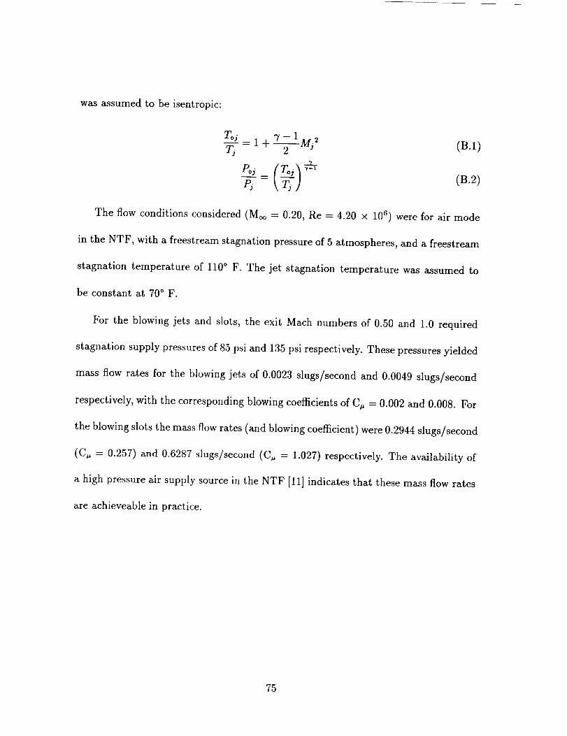
was assumed to be isentropic:
Tj 1+ Mj 2 (B.1)
- kTj ] (B.2)
The flow conditions considered (Moo = 0.20, Re = 4.20 × 10⁶) were for air mode
in the NTF, with a freestream stagnation pressure of 5 atmospheres, and a freestream
stagnation temperature of 110 ° F. The jet stagnation temperature was assumed to
be constant at 70 ° F.
For the blowing jets and slots, the exit Mach numbers of 0.50 and 1.0 required
stagnation supply pressures of 85 psi and 135 psi respectively. These pressures yielded
mass flow rates for the blowing jets of 0.0023 slugs/second and 0.0049 slugs/second
respectively, with the corresponding blowing coefficients of C u = 0.002 and 0.008. For
the blowing slots the mass flow rates (and blowing coefficient) were 0.2944 slugs/second
(C u = 0.257) and 0.6287 slugs/second (C u = 1.027) respectively. The availability of
a high pressure air supply source in the NTF [11] indicates that these mass flow rates
are achieveable in practice.
75

C Active Suction Simulation
The modifications to the TLNS3D-MB code to simulate the sidewall suction are
described in this appendix. Figure 134 shows a partial view of a two-dimensional grid
adjacent to a simulated porous surface. The suction over a surface is simulated by
specifying a constant normal velocity, U_o, at the porous surface. Since TLNS3D-MB
is a finite volume code, the flow quantities are specified and computed at cell centers.
Thus it is necessary to modify the ghost cell values to properly simulate the flow
through the porous surface.
The normal wall velocity is determined from the specified surface transpiration
coefficient:
(pU)_ (C.1)cq- (pu)_
where negative Uw denotes suction,and positiveU_ denotes injection.The imposed
normal wall velocity is obtained by rearranging equation C.1 to obtain:
u,o= cq(pu)_ (c.2)pill
The density at the wall is set equal to the density at the first interior cell, j=2. The
Cartesian velocity components are determined as:
_ = u_ (c.3)
v,_ = U_on,, (C.4)
where n, and nu are the Cartesian components of the normal vector n. Lastly, the
76
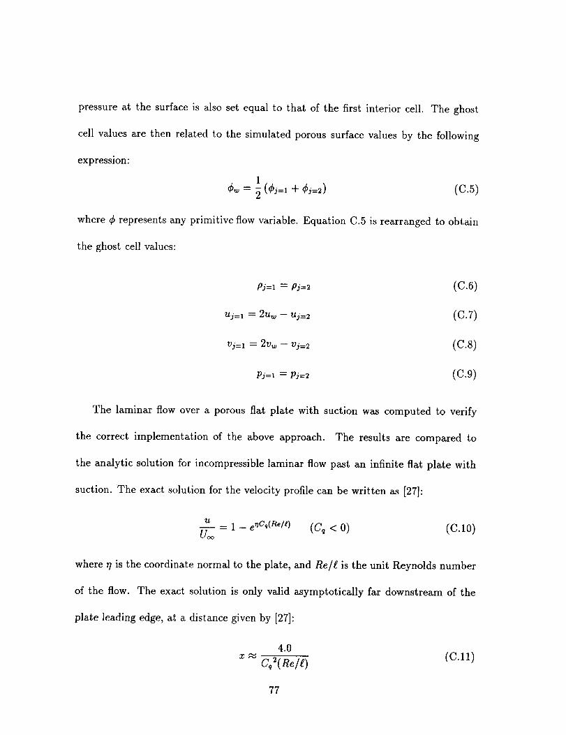
pressure at the surface is also set equal to that of the first interior cell. The ghost
cell values are then related to the simulated porous surface values by the following
expression:
1
¢_ = _ (¢j=, + Cj=_) (6.5)
where ¢ represents any primitive flow variable. Equation C.5 is rearranged to obtain
the ghost cell values:
Pj=I : Pj=2 (6.6)
Uj=1 : 2_ -- Uj=2 (6.7)
Vj=I = 2V_ -- Vj=2 (C.8)
pj=a = pj=2 (6.9)
The laminar flow over a porous flat plate with suction was computed to verify
the correct implementation of the above approach. The results are compared to
the analytic solution for incompressible laminar flow past an infinite flat plate with
suction. The exact solution for the velocity profile can be written as [27]:
tt
= 1 - e "cdRe/¢) (C, < 0) (C.10)
where r/is the coordinate normal to the plate, and Re/g is the unit Reynolds number
of the flow. The exact solution is only valid asymptotically far downstream of the
plate leading edge, at a distance given by [27]:
4.0
x _ uqt_t/e)'-'2'De'D, (C.11)
77

The following freestreamconditions wereused: Moo= 0.20, Re/g = 0.1 × l0 s
A unit length flat plate was examined, with grid dimensions of 129 × 33. Figure 135
compares the computed and Blasius [27] velocity profiles at the midpoint of the plate
for zero suction. The agreement is excellent, and indicates sufficient grid resolution.
For the given plate length and flow conditions, equation C. 11 indicates that an asymp-
totic behavior would be expected at x _ 0.4 with Cq = -.01. Figure 136 compares
the predicted velocity profile at the midpoint of the plate to the asymptotic solution
given by equation C.10. The agreement is excellent, and provides validation of the
implementation of the numerical boundary conditions. In addition, the convergence
characteristics of the code were not affected by the suction boundary condition.
To further examine the performance of the suction boundary condition, turbu-
lent two-dimensional flow over a backward facing sinusoidal ramp was examined.
The freestream conditions considered were: Moo = 0.20, Re/t. = 2.0 x 10⁶. The
one-equation Spalart-Allmaras turbulence model was employed. Figure 137 shows
a partial view of the grid, with the leading edge of the forward flat plate at z =
0.00. The grid dimensions were 145 x 65. Figure 138 shows the effect of suction,
applied only to the sinusoidal region. With no suction, Cq = 0.00, significant flow
separation is predicted. With the addition of suction, Cq = -.005, the extent of sepa-
ration decreases dramatically. Increasing the suction rate further, Cq = -.010, results
in a wholly attached flow field. As with the laminar flow computations, the suction
boundary condition did not introduce any numerical difficulties.
78

Tables
79

Table 1: Metric stand-off pressure tap locations
tap number tap number X/L1 26 0.49245
2 0.00027 27 0.51337
3 0.00134 28 0.53195
4 0.00403 29 0:54820
5 0.00877 30 0.56220
6 0.01516 31 0.57405
7 0.02244 32 0.58388
8 0.03058 33 0.59186
9 0.04220 34 0.59816
10 0.05721 35 0.60293
11 0.07519 36 0.60634
12 0.09565 37 0.60859
13 0.11851 38 0.61321
14 0.14375 39 0.62921
15 0.17109 40 0.66074
16 0.20015 41 0.70894
17 0.23057 42 0.76976
18 0.26194 43 0.83390
19 0.29378 44 0.89094
20 0.32562 45 0.93440
21 0.35699 46 0.96311
22 0.38741 47 0.97963
23 0.41648 48 0.98834
24 0.44385 49 0.99500
25 0.46924 50 1.00000
8O

Figures
81

100
5O
Reynolds 20Number
RN x 1g6 10
5
2
0.2
737-300
Ames 11 tlx 11 I!
RAE Bedlord 8 fl
1 Modane 8m
I I I I I0.4 0.6 0.8 1.0 1.2
Mach number
x8tl
Figure 1: Operating envelopes of several transonic wind tunnels (Reference [1]).
82
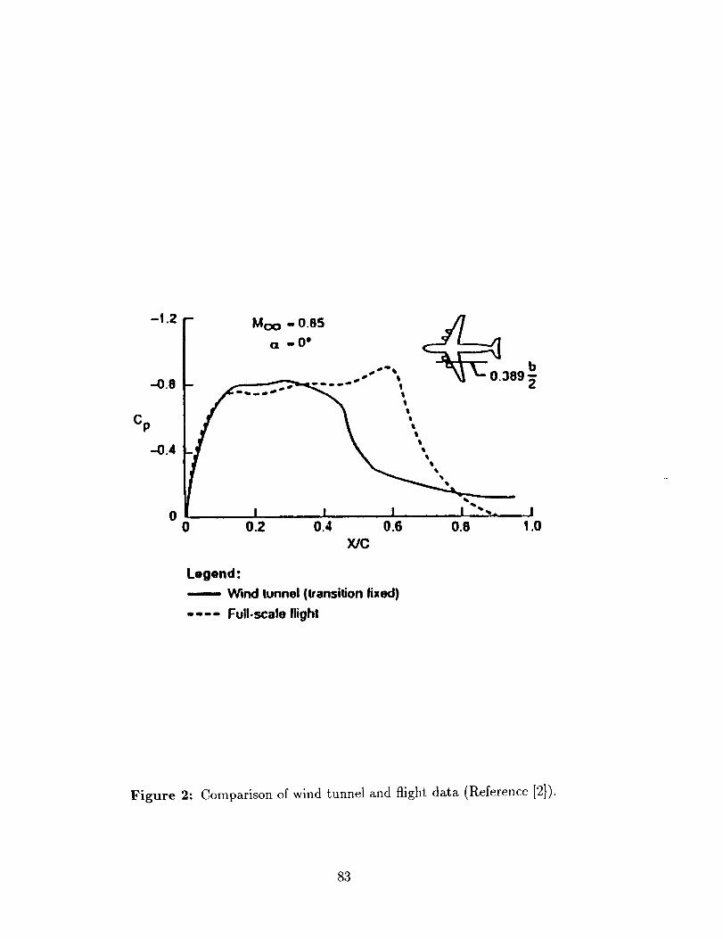
-f .2
-0.8
0
- Moo " 0.05 J7
°.0.
I 1 I ,, I ""-- l0 0.2 0.4 0.6 0.8 1.0
X/C
Legend:
-- Wind tunnel (transition fixed)
.... Full-scale flight
Figure 2: Comparison of wind tunnel and flight data (Reference [2]).
83

Figure 3: Comparisonof cruiseand high-lift configurations.
Figure 4: High-lift flow physics (Reference [3]).
84

Flow
Wind tunnel
sidewall
Figure 5: Comparison of full-span and semi-span models.
85

V_
j
r--
a) splitter plate mounting
b) sidewall mounting
Figure 6: Comparison of semi-span model mounting strategies (Reference [8]).
86

II
Figure 7: Planform view of semi-span model with stand-off geometry.
87

0.50
0.25
-0.25
-0.50
I
_11new leading edge location
I , _ = , I a , i i I , , I I
0.00 0.25 0.50 0.75 1.00
X/C
a) location of new leading edge
0.50
0.25
-0.25
-0.50 I , , , , I , , , , I
t.O0 0.25 0.50
X/C0.75 1.00
b) new tip airfoil
Figure 8: Construction of new tip airfoil.
88

0.50
0.25
-0.25
-0.50
open trailing edge
....... closed trailing edge
=.1095
I_''ll,_ I=,
0.00 0.25 0.50
WC
JllllJ
0.75 1.00
a) airfoil geometry comparison
3.00
2.00
1.00
X
0.00"0
-1.00
-2.00
-3.000,01
j upper surface
lower surface
-- open trailing edge
- - - dosed trailing edge
11= .1095
, , = , I , = , I , , _ , I , , , f I
0.25 0.50 0.75 1.00
X/C
b) airfoil slope comparison
Figure 9: Influence of trailing edge closure on root airfoil.
89

Y
Z
Figure 10: Oblique view of surface geometry.
._)0

Full-span
¥
Semi-span
Figure 11: Partial view of C-O grid topologies.
91

Figure 12: Aft fuselagesurfacegrid with sting.
92

a) grid
tunnel
sidewall1t
stand-off
fusel
wing trailing edge
Figure 13:
downstream.
b) block boundaries
Spanwise slice through semi-span grid at wing trailing edge, looking
93

\
\\
\
Figure 14: Streamwise slice through wing grid, r/= .2665.
94

\ II I
I
i
I
i
I
I
¥
Figure 15: Partial view of rectangular wing C-O grid.
95

-4.00
-3.50
-3.00
-2.50
-2.00Q.
-I .50
-I ,50
-0,50
0.50
0.50
1.00
TLNS3D
o EXPERIMENT289x73x73
i .......... 193x49x49
........ 5
0.00 0.25 0.50 0.75 1.00
X/C
(9
-4.00
-3.50
-3.00
-2.50
-2.00O.
-1.50
-1.00
-0.50
0.00
0.50
1.00
CFL3D
0.00 0.25 0.50 0.75 1.00
X/C
-4.00
-3.50
.3.00i
-2.50
-2.000.
(9 -1.so
-1.00
-0.50
0.00
0.50
1.00
INS3D
O
0.00 0.25 0.50 0.75 1.00
X/C
Figure 16: Influence of grid refinement on pressure distribution, r/ = 0.6084
(Moo = 0.14, a = 10.01 °, Re = 3.17x 10⁶).
96

C L
0.80
0.79
0.78
0.77
0.76
0.75
0.74
0.73
0.72
0.71
--O------ TLNS3D
.... " .... CFL3D
---O--- INS3D
0.70 , , , , I , , , , I , , , , r , , , , I
0.00E0 5.00E-6 1.00E-5 1.50E-5 2.00E-51/N
a) lift coefficient
0.060
0.050
C D
0.040
/ °/
/.. s_ _
0.030 .... i .... i .... i .... i0.00E0 5.00E-6 1.00E-5 1.50E-5 2.00E-5
1/N
a) drag coefficient
Figure 17: Influence of grid refinement on lift and drag coefficients (Moo = 0.14,
a = 10.01 ° , Re = 3.17 × 10⁶).
97

0.10
0.09
0.08
0.07
0 0.06_1_0.05
0.04
0.03
0.02
0.01
0.0'.00
TLNS3D
--c----_ 289x73x73
.... ° .... 193x49x49
--...... 97x25x2.5
/
/ .=("
• i
0.25 0.50 . 0.75 1.00 1.25ulU
0.10
0.09
0.08
0.07
._0.06
0.05
0.04
0.03
0.02
0.01
008:
0.10
0.09
0.08
0.07
0.06
0.05
0.04
0.03
0.02
CFL3D
/
...at"
0.25 0.50 0.75 1.00 1.25U/Uoo
INS3D
,//
/ ..a,"0.01 .._-_..I,,_
000 _ ..... L'-0. )0 0.25 0.50 , .0.75 1.00 1.Z5
u/UFigure 18: Influence of grid refinemenf°on upper surface streamwise velocity profile
at x/c = 0.50, 7/ = 0.6084 (Moo = 0.14, a = 10.01 °, Re = 3.17 × 10⁶).
98

0.20
0.00
y
1.50 -
1.00
C L
0.50
Q
0.00 _ ' '0.0
• EXPERIMENT
TLNS3D
---[]--- CFL3D
----_--- INS3D
J I , , , _ I , J j _ I , _ , , I
5.0 10.0 15.0 20.0
a, (deg.)
Figure 19: Comparison of predicted lift and drag coefficients to experimental data
(Moo = 0.14, Re = 3.17 × 10⁶).
99

-4.00 -
"q= .3436l
_3150
-_ o EXPERIMENT-3.00 -,_lq - TLNS3D
.2.55- I°_lo_ .......... CFL3D-2.00-_ - ....... INS3D
O -1.50-1.00
-0.50
0.00
0.50
1.00 ........0.00 0.25 0.50 0.75 1.00
X/C
-4.00TI = .6084
-3.50 :
-3oo;.25o
200 f '
(._ -1.50 1 1 °_
1
0.00 0.25 0.50 0.75 1.00
X/C
-4.00
-3.55
-3.00
-2.50
-2.00
-1.50
-1.00
-0.50
0.00
0.50
1.00
Figure 20: Comparison of predicted and
(Moo = 0.14, a = 10.01 °, Re = 3.17 × 10⁶).
"q= .9883
o o o,_- .
).00 0.25 0.50 0.75 1.00
X/C
experimental pressure distributions
100

1.00
0.75
C n 0.50
0.25
o .o_
TLNS3D
......... CFL3D
i i i J l [ i _ , I . , , _ | , _ , , J
:)0 0.25 0.50 0.75 1.00
q
Figure 21: Comparison of predicted spanwise load distributions (Moo = 0.14,a = 10.01 ° , Re = 3.17 × 10⁶).
lOl

0.10
0.09
0.08
0.07
(_ 0.06
0.04
0.03
0.02
0.01
oO .oo
11= 0.6084
---o----- TLNS3D
.... ° .... CFL3D
---_'---INS3D
,_ I ,
0.25 0.50 0.75 1.00
u/Uoo
Figure 22: Comparison of upper surface streamwise velocity profiles at x/c = 0.50
(M_o = 0.14, a = 10.01 ° , Re = 3.17 × 10⁶).
102

1.05 1
1.00
CL
Ckf
0.95
TLNS3D
--- - CFL3D
.... INS3DINS3D CFL3D
(1.67 hr.) (2.70 hr.)
. .__. Lift
'-:- T
., . ; ..... ..... Dracl
li /I '\ /
t i,,j
- 1.10
1.05
Co
CDf
1.00
o._,._,,,'o' ...... '"'" 8:_._'1. 2.0 3.0 4.0 5.0 6.0 7.0
Time (Y-MP hours)
Figure 23: Comparison of convergence histories (Moo = 0.14, a = 10.01 °,
Re = 3.17 × 10⁶).
103

-2.50
-2.00
-1.50
-1.00
-0.50
0.00
0.50
1.00
0.00
11= .2665
o EXPERIMENT
- TLNS3D
.......... CFL3D
........ INS3D
J a .... J
025 0.50 0.75 1.00
X/C
-2.50
-2.00
-1.50
¢_-1.00
O-0.50
0.00
0.50
1.00
11=.6234
0_0_ 025 0_0 0_5 I_0X/C
-2.50
-2.00
-1.50
r.-1.00
O-0.50
0._
0.517
1.00
11= .9066
J .... = , , i , I I I
0.00 0.25 0.50 0.75 1.00
X/C
Figure 24: Comparison of predicted and experimental pressure distributions
(M_ = 0.20, c_ = 4.43 °, Re = 4.20 x 10⁶).
104

1.00
0.75
O n 0.50
0.25
TLNS3D
......... CFL3D
....... INS3D
0(_ , , , , I .... I , , , , I ....0. .00 0.25 0.50 0.75
111.00
Figure 25: Comparison of predicted spanwise load distributions (,k£_ = 0.20,
a=4.43 ° , Re=4.20 × 10⁶ )
105

0.50
0.40
¢,_ 0.30
q = .6234
--o_ TLNS3D
.... '_.... CFL3D
---_'---INS3D
0.20 /
0.10 /
000 --- -- ' ' ' -- ' .... '"0.00 0.25 0.50 0.75 1.00 1.25
u/Uoo
Figure 26: Comparison of upper surface streamwise velocity profiles at x/c = 0.50
(Moo = 0.20, a = 4.430 , Re = 4.20 x 10⁶).
106

-2.50
-2.00
-1.50
-1.00
Q..
(_ -0.50
0.00
0.50
1.00
zI = .2665
o EXPERIMENT
241 x65x81'r'_,
......... 241x65x41
= -- .... 121x65x41
_ ...... 121x33x41
1.00 0.25 0.50 0.75 1.00X/C
-2.50
-2.00 I
-1.50 _"
-1.00 t
o5o E-l
0.00
0.50
1.00
_1= .6234
i, ] , , , , J , . . i I , , . , = .... I
).00 0.25 0.50 0.75 1.00
X/C
-2.50 ,-
-2.00-
-1.50 -
-1.00Q.
O -o5o
0.00
0.50
1.00
= .9066
O" 0 ....
0
0.00 0.25 0.50 0.75 1.00
X/C
Figure 27: Comparison of computed pressure distributions with experimental data
(Moo = .20, a = 4.43 ° , Re = 4.20 x 10⁶).
107

0.10241x65x81
0.00 ---o--- 241x65x41
-- - "_ " -- 121x65x41
0.08 --'"<>'"-- 121x33x41
0.07
0.06
0.05
0.04
0.00 __ _ "-, . _ .... J . , , , I0.00 0.25 0.50 0.75 1.00 1.25 1.50
u/U_
a) velocity profile, x/c = 0.50.
Cf
0.015 - I
0.010
0.005
0.000
-0.005
241x65x81
....... 241X65X41
...... 121x65x41
....... 121x33x41
I
.......
I .... I .... I , , , , I .... I
0,00 0.25 0.50 0.75 1.00
x/c
b) skin friction distribution.
6.00
5.00
4.00
y+3.00
2.00
1.00
0.00
-- 241x65x81
....... 241x65x41
121x65x41
....... 121x33x41
l ii ./.1..f .......... ....
I ._o_'_''._ j '
I .... I .... I , i i z I i i i i I
0.00 0.25 0,50 0.75 1.00
x/c
c) yplus distribution.
Figure 28: Influence of grid refinement on upper surface wing boundary layer,
r/ = 0.9066 (Moo = 0.20, a = 4.43 °, Re = 4.20 x 10⁶).
108

-2.50
-2.00
-1.50
-1.00(3.
0.0.50
0.00
0.50
1.00
11 = .2665
,, o EXPERIMENT
-- S-A
' ......... B-L
0.00 0.25 0.50 0.75 1.00X/C
C_1.00 "',,
0.00 0.25 0.50 0.75 1.00
X/C
-2.50
q = .9066
-2.00
-1.5(
-1.0( i
o..
0.0.5 ( o" _=....
0.00
0.50
0.00 0.25 0.50 0.75 1.00X/C
Pigure 29: Influence of turbulence model on computed pressure distributions
(M_ = .20, a = 4.43 ° , Re = 4.20 × 10⁶).
109

a) Baldwin-Lomax
a) Spalart-Allmaras
Figure 30: Influence of turbulence model on near surface streamline patterns
(Moo = 0.20, a = 12.55 ° , Re = 4.20 x 10⁶).
110

0.25
C M 0.00
Z
-0.25 , ,
C L
2.00
I.N
1.00
0.50
---O----- Full-span (Ames)
- - I- - - Full-ipa_ (T-LN_-MI.)
0.00 , , __ 1 ____ , I , , , , I , , , , J
0.0 5.0 10.0 15.0 20.0
a, deg.
Figure 31: Comparison of computed and experimental full-span lift and pitching
moment coefficients (Moo = .20, Re = 4.20 × 10⁶).
111

-2.50
-2.00
-1.50
-1.00O.
rO .0.50
0.00
0.50
1.00
xi= .2665o EXPERIMENT
i S3D-MB
0.00 0.25 0.50 0.75 1.00
X/C
-2.50
-2.00
-1.50
-1.00
O.
0 -o.50
11 = .6234
0.50_-
1.00 _- , ......... , .... _ .... ,0.00 0.25 0.50 0.75 1.00
X/C
-2.50
-2.00
-1.50
-I .00
0,,,
0 _.50
=.9066
0.50
1.00 _ ...... I .... L .... I ....0.00 0.25 0.50 0.75 1.00
X/C
Figure 32: Comparison of computed and experimental full-span pressure distribu-
tions (Moo = .20, _ = 4.43 °, Re = 4.20 x 10⁶).
112

-5.00 -
.,4.00-
-3.00 -
(_-2.00
-1.00
0.00-
1.00 -_J__ _0.00 0.25 0.50 0.75 1.00
1] = .2665
o EXPERIMENT
-- TLNS3D-MB
X/C
-5.00
-4.00
-3.00
(._-2.00
-1.00
000
100
11 = .6234
.......... _o.... o_0.00 0.25 O. 5 1.00
X/C
-5.00 -=.9066
-4.00 -
-300
i
C._-2.00<
-1.00
0.00
1.00 _ _ • • _ .... i .... i0.00 0125 0.50 0.75 1.00
X/C
Figure 33: Comparison of computed and experimental full-span pressure distribu-
tions (Moo= .20, c_ = 8.58 °, Re = 4.20 x 10⁶).
113

-8.00 :
-7.00 i
-6.00
-5.00 : o
C) 400E
-8100:-
-2.00
-1.00
0._
1.0t?
•rl = .2665
o EXPERIMENT
TLNS3D-MB
I , , =
0.00 0.25 0.50 0.75 1.00
X/C
lei _ r"
_ T1 = ._--_4-7.00
-6.00
-5.00
-4.00
-8.00
-7.00
-6.00
-5.00
-4.00EL
rO -3.00
-2.00
-1.00
0.00
1.00
q =.9066
- J .... i . , , , I .... J .... I
0.00 0.25 0.50 0.75 1.00
X/C
Figure 34: Comparison of computed and experimental full-span pressure distribu-
tions (Moo = .20, c_ = 12.55 °, Re = 4.20 x 10⁶).
114

C M
0.25
0.00
-0.25 J , ,
C L
2.00 -
1.50
1.00
0.5o
0.000.0
--o----- Semi-span (NTF,uncorrected)
- - -m- -. Semi-span (TLNS3D-MB)
, Jm"_ ,/
/ /
///
, , , , I , , , , I , , , , I , , , , I
5.0 10.0 15.0 20.0
a, deg.
Figure 35: Comparison of computed and experimental semi-span lift and pitching
moment coefficients (Moo = .20, Re = 4.20 × 10⁶).
115

-5.00
-4.50
-4.00
-3.50
-3.00
-2.50
O'_-0o-1.50
-1.00
-0.50
0.00
0.50
1.00
_1= .2665
o EXPERIMENT (UNCORRECTEB)
TLNS3D-MB
: i
0.00 0.25 0.50 0.75 1.00
X/C
-5.00 [
-3.50
-3.00
-2.50
(J_2- .00
-1.50
-0.50
0.00
0.50
1.00
11= .6234
).00 0.25 0.75 1.00
X/C
Figure 36: Comparison of computed and experimental semi-span pressure distribu-
tions (Moo = .20, a = 8.24 °, Re = 4.20 × 10⁶).
116

-1.00
-0.80
-0.60
-0.40
-0.20
Cp o.oo
0.20
0.40
0.60
0.80
1.00
q =-.0437
• o EXPERIMENT(UNCORRECTED)
TLNS3D-MB
)
wingroot
I , _ , , I _ a _ , I _ , , _ I _ _ _ _ I
0.00 0.25 0.50 0.75 1.00
X/L
Figure 37: Comparison of computed and experimental semi-span pressure distribu-
tions (M_ = .20, a = 8.24 ° , Re = 4.20 x 10⁶ ) .
117

CM
0.25
o.0o
-0.25
.. /_0
I I I _ I
2.00
1.50
0.50
Full-span(Ames)
----o--- Semi-span(NTF,uncorrected)
- - 41- -- Full-span(TLNS3D-MB)
- - 4- -- Semi-span(TLNS3D-MB)
/
!
0.000.0 5.0 10.0 15.0 20.0
deg.
Figure 38: Comparison of full-span and semi-span lift and pitching moment coeffi-
cients (Moo = .20, Re = 4.20 x 10⁶).
118

-2.50
-2.00
-1.50
-1.00
0 -0.50
0.00
0.50
= .2665
Full-span
_ ° ........ Semi-span
1.00I .... I .... O. /5 I .... I0,00 0.25 0 0,75 1.00
X/C
O
-2.50
-2.00
-1.50
-1.00EL
-0.50
0.00
0.50
1.00
= .6234
..... i .... io_o.... o_5 o._o 0.75 looX/C
-2,50TI = .9066
-2.00
"'50-1 .(_
EL
0 -0.50
0.00
1.00o.;o....o_5....o._o....o._s....I._o
X/C
Figure 39" Comparison of computed full-span and semi-span pressure distributions
(Moo = .20, _ = 4.43 °, Re = 4.20 x 10s).
119

-5.00 -_1 = .2665
4.00 - Full-span
?, ......... Semi-span
-3.00 _,_,
-2.1_
-1.110
0._
1.00 _ ...... I , , , , I , --
0.00 025 0.50 0.75 1.O0
X/C
-5.00
-4.00
-3.00
-2.00
-I .00
0.00
1.00
TI = .6234
I , , , , i .... i .... i .... a
0.00 025 0.50 0.75 1.00
X/C
-5._ -_=.9_6
-4,00 -
-3.00 -
-2.00
-I .00
0.00
1.000.00 025 0.50 O. 5 1.00
X/C
Figure 40: Comparison of computed full-span and semi-span pressure distributions
(Moo = .20, a = 8.58 ° , Re = 4.20 × 10⁶).
120

-8.00
-7.00
-6.00
-5.00
-4.00t-t
0 -3,oo
-2.00 __'_
-1.00 _ _...._..._._
0.00 _-J
1.00 _ ..... _ .... , ....0.00 02.5 0.50
X/C
tl = ,2665
-- Full-span
......... Semi-span
o. 5
-8.00
°7,00
-6.00
-5.00
r_ -4.00
0 -3oo
-2.00
-1.00
0.00
'q = .6234
1.00-A ....................0.00 0.25 0.50 0.75 1,00
X/C
-8.00
-7.00
-6.00
-5.00
-4.00
0 -3.oo
-2.00
-I.00
0.00
1,00
11= .9066
3
f
0.00 0.25 0.50 0.75 1.00
WC
Figure 41: Comparison of computed full-span and semi-span pressure distributions
(Moo = .20, a = 12.55 ° , Re = 4.20 × 10⁶).
121

-0.50
-0.40
-0.30
'_.20
-0.10
0.00
0.10
"rl= .2665
lower sudace
......... upper surface
:,,
0.00 o_.... o._o o._5.... 1_oX/C
-0.50
-0.40
-0.30
¢z.
-0.10
0.00
0.10 = .... = ....0.00 0.25
11= .6234
0.50 '0. 5
X/CI
1.00
-0.50
-0.40
-0.30
_ -0.20
-0.10
0.00
0.10
TI = .9066
,h
0.00 O. 5 0.50 0.75 1.00
X/C
Figure 42: Computed differential wing pressure distributions (Moo = .20, a = 8.58 °,
Re = 4.20 × 10⁶).
122

O n C
2.00 -
1.75
1.50
1.25
C 1.oo
0.75
0.50
0.25
0.000.00
Full-span
a = 12.55 ° ....... Semi-span
0.25 0.50 0.75 1.00
11
Figure 43: Comparison of computed spanload distributions (Moo = .20 ,
Re = 4.20 x 10⁶).
123

-1,00
-0.80
q = 0.00
-- Full-span
....... Semi-span
-0.60
-0.40 "l
o.o°'°r4 Fw'ngr°°'I
1.00 t .... i .... _ .... p .... i
0.00 0.25 0.50 0.75 1.00
X/L
a) c_ -- 4.43 °
-1,00
-O.BO
-0.60
-0.40
-0.20
Cp o.oo
rl = 0.00
-- Full-span
....... Sem!-spsn
0.20 !
0.40
0.60
O.t_ -
i
t - .*'k
1.00 i .... i .... i .... i .... i
0.00 0.25 0.50 0.75 1.00
X/I_
b) a = 8.58 °
-I.00 -
-0.80 -
-0.60 L
-0.40
-0.20
Cp ooo_i0.20 :-
0.40-
0.80-
0._='
q = 0,00
-- Full-span
....... Semi-span
,,i
• • • se
" I .... i .... , .... 1 .... J
0.00 0.25 0.50 0.75 1.00
X/L
c) a = 12.55 °
Figure 44: Comparison of computed full-span and semi-span fuselage centerline
pressure distributions (Moo = 0.20, Re = 4.20 × 10⁶).
124

a) a = 4.43 °
b) a = 8.58 °
c) a = 12.55 °
Figure 45: Comparison of computed full-span and semi-span upper wing surface
streamline patterns (Moo = 0.20, Re = 4.20 x 10⁶).
125

¥
Z
a) full-span
¥
Z
b) semi-span
Figure 46: Comparison of computed full-span and semi-span fuselage streamline
patterns (Moo = 0.20, a= 12.55 ° , Re = 4.20 x 10⁶).
126

Figure 47: Planform view of streamline patterns on upper surfaceof semi-spanconfiguration (M_ = 0.20, c_ = 12.55 °, Re = 4.20 x 10⁶).
127

0.75
0.50
0.25
..J
0.00
-0.25
-0.50
-0.75-0,25
I I I ' I , , , , I | i , • I , , . , I = i
0.00 0.25 0.50 0.75
X/L
t = I , , , , I
1.00 1.25
a) full-span
0.75 -
0.50
0.25
-0.25
-0.50
, t t i I , • , , I , , i , I , , ' ' I , , , _ I • . , , I
0.00 0.25 0.50 0.75 1.00 1.25
X/L
b) semi-span
Figure 48: Comparison of computed full-span and semi-span root plane streamline
patterns (M_ = .20, c_ = 4.43 °, Re = 4.20 × 10s).
128

0.75
0.50
0.25
-0.25
-0.50
-0.75-0.25
I I I = I I ' ' ' I , , _ = I = , = = I = i . • I , • . , I
0.00 0.25 0.50 0.75 1.00 1.25
X/L
a) full-span
0.75 -
0.50
0.25
0.00
-0.25
-0.50
i ' ' ' I , , , , I _ = = , I i i ' ' I , , , , I = , = , l
0.00 0.25 0.50 0.75 1.00 1.25
X/L
b) semi-span
Figure 49: Comparison of computed full-span and semi-span root plane streamline
patterns (Moo = .20, _ = 8.58 °, Re = 4.20 × 10⁶).
129

0.75
0.50
0.25
0.00
-0.25-0.50
-0.75-0.25 0.00 0.25 0.50 0.75 1.00 1.25
X/L
a) full-span
0.75
0.50
0.25
_>_.0.00
..............................2 0.00 0.25 0.50 0.75 1.00 1.25
X/L
b) semi-span
0.15
0.10
0.05
_>_.0.00
-0.05
-0.10
-0.15-0.15
.... i .... r .... I .... i .... i . , i 1_'-"I-0.10 -0.05 0.00 0.05 0.10 0.15
X/L
c) semi-span nose region
Figure 50: Comparison of computed full-span and semi-span root plane streamline
patterns (Moo = .20, a = 12.55 °, Re = 4.20 × 10⁶).
130

Figure 51: Comparisonof computedsidewallstreamlinepattern and experimentaltuft visualization results (Moo= .20,a = 8.24 °, Re = 4.20 x 10⁶).
131

0.10
0.09
0.08
0.07
0.06
_0.05
0.04
0.03
0.02
0.01
0.00,
0.00
"rl= .2665
Full-span
.... n .... Semi-span
[
_---..._RIZ_Cr. I __ . . I .... Z .... I
0_5 0._ 0._ 1.06 1_ 1._
u/U_
0.10
0.09
0.06
0.07
0.06
_0.05
0.04
0.03
q = .2665
Full-span
.... a--- Semi-span
0.020.01
0.06 ..i .... I. 1 .i. t .... i .... i
-0.25 -0.20-0.15 -0.10 -0.06 0.06 0.05 0.10 0.15 0.20 0.25
w/I.l.
0.10
0.09
0.08
0.07
0.06
_0.05
0.04
0.03
0.02
0.01
0.06
0.00
"q= .6234+ Full-span
.... a .... Somi-spen
0.25 0.50 0.75 1 .CO 1.25 1.50
U/I.l.
O.lO ::1 "q= .62340.09 , I _ Full-sl_ n
0.08 '_ I .... o .... Semi4pan
0.07
0.06
K3
0.05
0.04
0.0_
0.02
0.01 i
0.06 ,.,i,, ...i .... i .... t .... i .... ,-0.25 -0.20 -0.15 -0.10 -0.05 0.00 0.05 0.10 0.15 0.20 0.25
w/U.
0.10
0.09
0.08
0.07
0.06
_0.05
0.04
0.03
0.02
0.01
O.C_
11 ----- .9066
Full-span
.... o .... ,serni_
0.06 0.25 0.50 0.75 1.00 1.25 1.50
u/U_
a) streamwise
0.10
0.09
iii;,0.06
_, 0.05
0.04
11 = .g066
Full,._oan
.... a .... Semi_
0.03 - "_
0.01
0.00 ,,,I,,,. .,..i .... i .... i .... I .... i-0.25 -0,20 -0.15 -0.10 -0.05 0.06 0.06 0.10 0.15 0.20 0.25
w/U.
b) spanwise
Figure 52: Comparison of full-span and semi-span upper surface wing velocity pro-
files at x/c = 0.50 (Moo = 0.20, a = 8.58 °, Re = 4.20 × 10⁶).
132
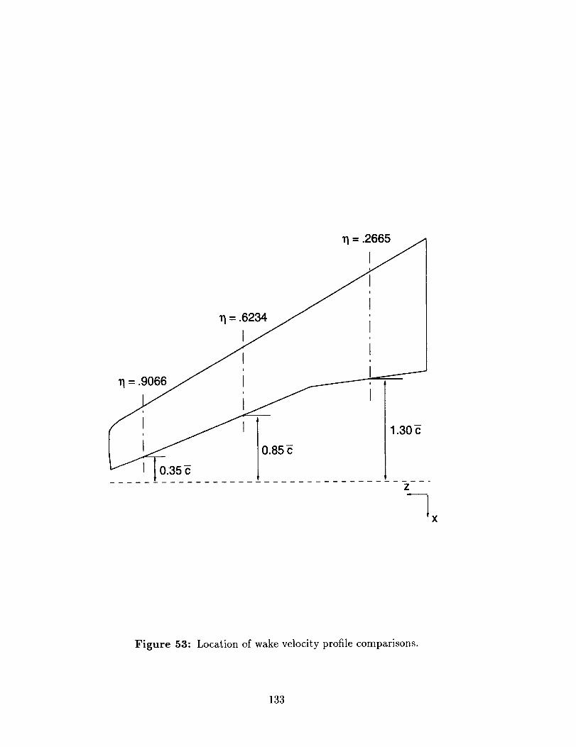
0.3s_ 1 1 .Z
,.o--
1×
Figure 53: Location of wake velocity profile comparisons.
133

1.00
0.75
0.50
0.25
I00.00
-0.25
-0.50
-0.75
-I.000.50
11= .2665
-- Full-span
....... Semi-span
J
0.75 1.00
u/U=
, , I125
1.00
0.75
0.50
0.25
0.00
-0.25
-0.50
-0.75
-1.000.50
= .6234
-- Full-span
....... Sen_-span
i__ . . i i
0.75 1.00
u/U.
I
1.25
1.oo 11= .9066 [-- Full-sign
0.75 ....... Semi-span
0.50
0.25
0.00
-0.50
-0.75
0.50 0.75 1.00 1.25
u/U.Figure 54: Comparison of full-span and semi-span wake velocity profiles (M_ = .20,
a = 8.58 ° , Re = 4.20 x 10⁶).
134

-9.00
q_-8.00
-7.00
-6.00 L-
-5.00 _-
(..)_-4.00
-3.00
-2.00
-1.00
0.00
1.0( , .... ,0.00 0.25
= .2665
EXPERIMENT (UNCORRECTED)
TLNS3D-MB
_o
0.50 O. 5 1.00
X/C
-9.00
-8.00
-7.00
-6.00
-5.00
C,)_-4.00i
-3.00
-2.01)
-1.00
0._
1.00
%
11= .6234
o
o
°o 0
_-____° ° o
i .... i . , , , i .... L , I , , I
0.00 0.25 0.50 0.75 1.00
X/C
Figure 55: Comparison of computed and experimental semi-span pressure distribu-
tions (Moo = .20, a = 18.25 °, Re = 4.20 x 10⁶).
135

0.50
CM
0.25
0.00
-0.25 I I I
2.00
1.50
C L I.oo
0.50
Full-span(Ames)
Semi-span(NTF,uncorrectecI)
• Full-span (TLNS3D-MB)
• Semi-span(TLNS3D-MB)
!
0.000.0 5.0 10.0 15.0 20.0
a, deg.
Figure 56: Comparison of full-span and semi-span lift and pitching moment coeffici
ents (Moo = .20, Re = 4.20 × 10⁶).
136

11= 2665
Full-span
......... Semi-span
-9.00
-8.00
-7.00
-6.00
-5.00
°=400
-3.00
-2.00
-1.00
0.00
1.00 I , , , , I , , , , l .... I , , ,
0.00 0.25 0.50 0.75 '1._00
X/C
-8.00
-8.0(
-7.0(
-6.00
-5.00
-4.00
-3.00
-2.00
-1.00 _ __
0.00
1.00 _ .... , .... , ....
0.00 0.25 0.50
X/C
11= .6234
0.'5"7 " ' ' f1.00
-9.00
-8.00
-7.00
-6.00
-6.00
-3.00
-2.00
-1.00
0.00
1.0¢
_=.9_6
j
i , . . i I , , , , i , , , , i . , , , i
0.00 025 0.50 0.75 1.00
X/C
Figure 57: Comparison of computed full-span and semi-span pressure distributions
(Moo = .20, a = 18.25 °, Re = 4.20 × 10⁶).
137

-0.75 I ....
-0.50" l --
-0.25
ACp 0.50
0.25
0.50 i .... , .... i .... i .... JL00 0.25 0.50 0.75 1.00
X/C
-0.75
-0.50
-0.25ACPooo. .......
0.25
0.5(, L , .... t .... i .... J .... J0.00 0.25 0.50 0.75 1.00
X/C
-0.50
•0.75 ................ TI= '6234 1
-0.25
ACpo.oo
0.25
0.500.00 0.25 0.50 0.75 1.00
X/C
-0.75
-0.50
-0.25
ACpo.oo
............. .... TI!= 16234
050o._o.... 0;5I 1 .... I
0.75 1.000.50
X/C
-0.75 ....... 1'1= .9066 ....
-0.50
-0.25
ACp o.oo --_
X/C
a) upper surface
-0.75 I
-0.50 1
= .9066
0.25
0.503.00 0.25 0.50 0.75 1.00
X/C
b) lower surface
Figure 58: Computed differential wing pressure distributions (Moo = 0.20,
a= 18.25 ° , Re=4.20 × 10⁶).
138

-1.00
-0.80
-0.60
-0.40
-0.20
Cp o.oo
0.20
0.40
0.60
0.80
1.00
i
II
I
I
I
|
I
I
q =0.00
Full-span
....... Semi-span
: ,_V,
.'_-_ ,, .-_-'/ "3_1
{ _/ _t/' v _ wing root '
0.00
.... I .... I , , , , I , , , , I
0.25 0.50 0.75 1.00
X/L
Figure 59: Comparison of computed full-span and semi-span fuselage centerline
pressure distributions (Moo = .20, a = 18.25 °, Re = 4.20 × 10⁶).
139

a) full-span
b) semi-span
Figure 60: Comparison of computed upper wing surface
(Moo = .20, c_ = 18.25 °, Re = 4.20 x 10s).
streamline patterns
140

-0.75
-0.25 0.00 0.25 0.50 0.75 1.00 1.25
X/L
0.75
a) full-span
0.50
0.25
-0.25
-0.50
-0.75 , , • _ I = , , , I , . i i I , , , , I .... I i , , , I
-0.25 0.00 0.25 0.50 0.75 1.00 1.25
X/L
b) semi-span
Figure 61: Comparison of root plane streamline patterns (Moo = 0.20, ct = 18.25 °,Re = 4.20 x 10⁶).
141

o.ooFI
I I_ tunr_l sidewall
s.ool-I ::_ tunnel sidewJ
c-:_,O.OC
N
I !.10.00 f _ , . , I , , , , i .... I .... 1
-5.00 0.00 5.00 10.00 15,00
Y (in.)
a) h = 156"
C_,0.00
N
0.00 5.OO
Y (in.)
b) h=56"
10.00 15.00
10.00 10"00 II t5.00 ]-- 5.00 _-
funnel sidewall
N N
.5 .o_
*
-10.00 -10.00-5.00 0.00 5.00 10.00 15.00 -5.00 0.00 5.00
Y (in.) Y (in.)
c) h=26" d) h= 16"
10.00 15.00
Figure 62: Frontal view of various stand-off heights examined.
142

CL
1.20
1.19
1.18
1.17
1.16
1.15
1.14 q
1.1:
1.1;
1.11
1.100.00
• Full-span
- - -(3 - - Semi-span
_0 _
i!
p", full-span
0
_0
' ' ' , I i , i , I , , , _ I
5.00 10.00 15.00
h/8"
a) lift coefficient
0.00
C M
-0.01
-0.0_ ;
.0.03
.0.04
-0.05
-0.06
-0.07
.0.08 (
"0.09
.0s
s
s
s
,,0 _
/i
i
O"s
full-span
-0.10 ' , , , , _ _ , , I , i , , I
0.00 5.00 , 10.00 15.00
b) pitching moment coefficient
Figure 63: Influence of stand-off height on lift and pitching moment coefficients
(Moo =0.20, a=8.58 ° , Re=4.20 x 10⁶).
143

,0'5°" ........ 1"1= .2665
-o.4o h = 158"[
i
......... 1,,0.30 h=28. l
h=18 I
-0.10 , : :
r0,00
0.10 i .... _ .... i .... i0.00 0.25 0,50 0.75 1.00
X/C
-0.50
-0.40
-0.30
ACp_.2°
-0.10
0.00
0.10
.... 'q = .2665
il , , J , .... i
L00 0.25 0,50 0.75 1.00X/C
ACp,0.2o
-0.10
0.00
0.10
-0'50 1 ...... .... 'q = :6234-o.401.............. i..........
,0.30
.............. _-.__
| . , , . I .... I .... I .... I
0.00 0.25 0.50 0.75 1.00
X/C
ACp'O-2O
,0.10
0.00
0.10
,0"50 ............... ...... 'q= '6234
.0.40.•: ............ .........
,0.30 ................ : .................
, , . . I .... I ....
L00 0.25 0.50
X/C
.... I
0.75 1.00
ACp ,0.2°
-0.10
0.10I . , , , I , , , , I t , • = j
0.00 0.25 0.50 0.75 1.00
X/C
a) upper surface
-0.30
ACp,0-2o
-0.10
-o.50 ............. : ...... n= :90_
.-0.40 ....... ......... : .............. i
: i
0.00 _ ::'-,.,_' '.
, , . , I , , , , I , , , , J0.10 ' .... I0.00 0.25 0.50 0.75 1,00
X/C
b) lower surface
Figure 64: Influence of stand-off height on differential wing pressure distributions
(Moo = 0.20, a = 8.58 °, Re = 4.20 x 10s).
144

1.50
1.25
1.00
C n C
C 0.75
0.50
0.25
0.000.00
• _ .-. Full-span
_('_ _'_,',.",, - ...... Semi-span:h= 15S
" = 58"I _'_,, ..... Semi-span: h
-, ......... Semi-span: h = 25"
_, - ...... Semi-span: h = 18"
0.25 0.50 0.75
111.00
Figure 65: Influence of stand-off height on spanload distribution (Moo = 0.20,
a = 8.58 °, Re = 4.20 × 10⁶).
145

-1.00
-0.80
-0.60
-0.40
-O.2O
Cp o.oo
0.20
0.40
0.60
0.80
1.000.00
Full-span
....... Semi-span: h = 158 °
..... Semi-span: h = 5_"
.... Serni-span: h = 26"
.........................Semi-span: h = 18
t
_ wing root
, _ ! • , , , !, , , I i i i i I ,
0.25 0.50 0.75 1.00
X/L
a) upper surface
• 1.00
-0.80
-0.60
-0.40
-0.20
Cp o.oo
0.20
._, 1_ /_ ...... J.,Y _¢.. 11 ..... .'/ _.-_I
0.40
0.60 I0.80
1,000.00
wing root
, , , I , , I, , i I , , , i I
0.25 0.50 0.75 1.00
X/L
b) lower surface
Figure 66: Influence of stand-off height on fuselage centerline pressure distribution
(Moo = 0.20, c_ = 8.58 °, Re = 4.20 × 10⁶).
146

a) full-span b) semi-span: h = 156"
c) semi-span: h = 26*
Figure 67: Influence of stand-off height on wing upper surface streamline patterns
(Moo = 0.20, a = 8.58 °, Re = 4.20 x 10⁶).
147

a) full-span
,(
¢__xZ
b) semi-span: h = 15_*
¥
Z
c) semi-span: h = 2_*
¥
2
Figure 68: Influence of stand-off height on fuselage streamline pattern (M_ = 0.20,
= 8.58 °, Re = 4.20 x 10⁶).
148

0.75
0.50
0.25
0.00 0.25 0.50 0.75
X/t.
a) full-span
0.75
0.50
0.25
_>_.0.00
-0.25
-0.50
-0.751.00 1.25 -0.25 0.00 0.25 0.50 0.75 1.00
X/L
b) semi-span: h = 15_*
1.25
0.75
0.50
0.25
0.00 0.25 0.50 0.75
X/L1.00
c) semi-spa,n: h = 2_*
Figure 69: Influence of stand-off height on root
(Moo = 0.20, a = 8.58 °, Re = 4.20 x 10⁶).
1.25
plane streamline patterns
149

0.25
C M o.oo
-0.25
.0/
/
// /
sss_
2.00
1.50
C L 1.oo
0.50
0.000.0
---o---- Full-span
- - -o- - - Semi-span: h = 156"
• Semi-span: h = 26
.Q
,S/
¢7
5.0 10.0 15.0 20.0
a, deg.
Figure 70: Influence of stand-off height on semi-span lift and pitching moment
coefficients (Moo = .20, Re = 4.20 x 10s).
150

-0.50 ............Xl = .2665
-0.40
-0.30
:p-o.2o-0.10
0.00
0.10 J .... i .... i ....0.00 0.25 0.50
X/C
h= 158"
......... h=28"
, :-, ................. . ...........
0.75 1.00
-0.50
-0.40
-0.30
ACp-O-2O
-0.10
0.00
0.10
11= .2665
0.00 0.25 0.50 0.75 1.00
x/c
-0.50q= .6234
-0.40 ..... ..... : ....
-0.30 : .....
-0.10
0.10 J i .... _ .... , .... j0.00 0.25 0.50 0.75 1.00
X/C
....... j
i . , , , I
0.75 1.00
-0.50-:
-0.40
-0.30
ACp-O.2O-0.10
0+00
0.10 L_J_0.00
tl:= .9066
.................. - ......... ____-_._I I a , , , I , . , = I
0.25 0.50 0.75 1.00
X/C
a) upper surface
-0.50 ..... :........ : ....... .......11= .9066
•0.40: .... ....... .....
-0.30
ACp-0-2o
-0.10
L0.00 ...... -/_.
0.10 _ .... i .... , .... , .... i0.00 0.25 0.50 0.75 1.00
X/C
b) lower surface
Figure 71: Influence of stand-off height on differential wing pressure distributions
(Moo = 0.20, a =4.43 ° , Re=4.20 × 10⁶).
151

-0.70
-0.60
-0.50
-0.40
ACp °.50-0.20 !
-0.I0
0.00
0,I0
TI = .2665
0.00 0,25 0.50 0.76 1.00
X/C
-0.70
-0.60
-0.50
-0.40
ACp_.50-0.20
-0.10
0.00
0.10
=.2665
0.00 0.25 0.50 0.75 1.00
X/C
-0.70
-0.60
-0.50
-0.40
ACp_-50-0.20
'rI = .6234
-0"10 I
oool,.......0.10 0.00 .... 0.25' '0.50 0.75' 1.00
X/C
-0.70
-0.60
-0.50
-0.40
ACp _.50-0.20
-0.10
0.00
0.10
=.6234
l , q I l , , . = I
i.O0 0.25 0.50 0.75 1.00
X/C
-0.70
-0.60
-0.50
-0.40
ACp °.3°-0.20
-0,10
O.OC
0.10
=.9066
I.O0 0.25 0.50 0.75 1.00
X/C
a) upper surface
Figure 72:
(Moo = 0.20,
-0.70
-0.60
-0.50
-0.40
ACp _-50-0.20
-0.10
0.00 I
q = .9066
0.10 L t .... i .... l .... _i_ .......... I
0.00 0.25 0.50 0.75 1.00
X/Cb) lower surface
Influence of stand-off height on differential wing pressure distributions
c_= 12.55 ° , Re=4.20 x 10⁶).
152

-1.00 -
-0.80
-0.60
-0.40
-0.20
Cp o.oo,
0.20
0.40
0.60
0.80
1.00
"q= 0.00
Full-span
....... Semi-span: h = 155"
..... Semi-span: h = 25"
I x
- _,,r "_:+_+_'-_ __mI +V . +'_
I --'I +--wmro=tIi
I i J l i I i , I I I i i I i I + i l i I
0.00 0.25 0.50 0.75 1.00
X/L
Figure 73: Influence of stand-off height on fuselage centerline pressure distribution
(Moo = 0.20, a = 4.43 °, Re = 4.20 × 10⁶).
153
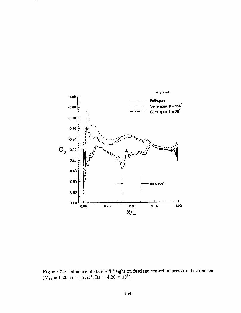
Cp
-1.00
-0.80
-0.60
-0.40
:0.20
0.00
0.20
0.40-
0.60-
0.8O i
11=e.ee
Full-span
....... Semi-span: h = 156"
,, Semi-span: h = 28I
I
---- wing root
1.00 i , , , , I _ _ n n I .... I , , , , I0.00 0.25 0.50 0.75 1.00
X/L
Figure 74: Influence of stand-off height on fuselage centerline pressure distribution
(Moo = 0.20, a = 12.55 °, Re = 4.20 × 10⁶).
154

a) full-span b) semi-span:h = 156"
c) semi-span:h = 26*
Figure 75: Influenceof stand-off height on wing upper surfacestreamlinepatterns(Moo= 0.20,a = 4.43 °, Re = 4.20 × 10s).
155

a) full-span b) semi-span: h = 15_*
c) semi-span: h = 26*
Figure 76: Influence of stand-off height on wing upper surface streamline patterns
(Moo = 0.20, a = 12.55 °, Re = 4.20 × 10⁶).
156

-0.75
-0.50
-0.25
ACpo.oo
0.25
71= .2665
h= 158 °
......... h=25
0.50 J- _j
0.00 0.25 0.50 0.75 1.00X/C
-0.75 ......
-0.50
-0.25
&CPo.oo
0.25
0.50
1] = .2665
0.00 0.25 0.50 0.75 1.00X/C
-0.25
ACPo.oo
"0"75 1 ..... 1]:=16234.-0.50 ,
i
t
;
0.25
0.50 ........0.00 0.25 0.50 0.75 1.00
X/C
-0.7!..............
11= .6234
-0.5( ..........
-0.25 ', .....
,
ACpo oo ;
..........................0.25
0.50 i .... i .... I .... i .... i0.00 0.25 0.50 0.75 1.00
X/C
-0.75
-0.50
-0.25
&Cpo.oo
0.25
=.9066
0.50 ___t .... i , , , __j0.00 0.25 0.50 0.75 1.00
X/Ca) upper surface
-0.25
&CPo.oo
0.25
'rl = .9066
0.50 _-_J- .... t , , , , _j
0.00 0.25 0.50 0.75 1.00X/C
b) lower surface
Figure 77: Influence of stand-off height on differential wing pressure distributions
(Moo =0.20, a= 18.25 ° ' Re=4.20 x 10⁶).
157

-1.00
-0.80
-0.60
-0.40
-0.20
Cp o.oo
0.20
0.40
0.60
0.80
1.00
11= 0.00
s,, Full-span
'_ ....... Semi-span: h = 158"I
' _ ..... Semi-span: h = 2_"I I
I 1
I t
t \. /
I , , i , I , = i , I , , , , I , i ' ' i
LO0 0.25 0.50 0.75 1.00
X/L
Figure 78: Influence of stand-off height on fuselage centerline pressure distributions
(Moo = 0.20, a = 18.25 °, Re = 4.20 x 10s).
158

a) full-span b) semi-span:' h = 15_*
c) semi-span: h = 26"
Figure 79: Influence of stand-off height on upper wing surface streamline patterns(Moo = 0.20, a = 18.25 °, Re = 4.20 x 10⁶).
159

Y
z
a) full-span
b) semi-span: h = 156"
¥
Z
c) semi-span: h = 26"
¥
Z
Figure 80: Influence of stand-off height on fuselage streamline pattern (Moo = 0.20,
c_ = 18.25 °, Re = 4.20 x 10⁶).
160

0.75 0.75
-0.25 0.00 0.25 0.50 0.75 1.00 1.25 -0.25 0.00 0.25 0.50 0.75 1.00 125
X/L X/L
a) full-span b) semi-span: h = 15_*
_,. 0.00
-0.25
-0.50
075i 0.50
0.25
-0.75-0.2! 0.00 0.2,5 0.50 0.75 1.00 1.25
X/L
c) semi-span: h = 26"
Figure 81: Influence of stand-off height on root plane streamline patterns
(M_ = 0.20, a = 18.25 ° , Re = 4.20 x 10⁸).
161

tunnelsidewall tunnelsidewall
a) nose, 2-D stand-off b) nose, 3-D stand-off
_-- tunnelsidewall
c) tail, 2-D stand-off
*-- tunnelsidewall
d) tail, 3-D stand-off
Figure 82: Comparison of 2-D and 3-D stand-off geometries.
162

CL
1.20
1.19
1.18:
1.17
1.1(
1.1,=
1.14 (
1.13
1.12
1.11
1.100.03
• Full-span
- - -0 - - Semi-span (2-13 stand-off)
z_ Semi-span (3-D stand-off)
s
J
_0 _
i
i
0
, full-span0
A
, , , , I , , , , I , , , , I
5.00 , 10.00 15.00
h/5
a) lift coefficient
0.O5
C M
-0.01
-0.02
-0.03
-0.04
-0.O5
-0.06
-0.07
-0.08 (
-0.09
-0.100.00
.0
p
,,0 _/
Ii
//
,o"full-span
A
5.03 10.00 15.00
h/5"
b) pitching moment coefficient
Figure 83: Influence of stand-off shape on lift and pitching moment coefficients
(Moo = 0.20, a = 8.58 °, Re = 4.20 × 10⁶).
163

-0.50 -
-0.40
-0.30
ACpO.2O
-0.10
0.00
0.10 _L, L0.00 0.25
TI= .2665
2-D......... 3-D
/
L I I
0.50 0.75 1.00
X/C
-0.50
-0.40
-0.30
ACp_.2°
-0.10
0.00
0.10
11= .2665
ii,
i i i • ___
0.00 0.25 0.50 0.75 1.00
X/C
-0.50
-0.40l
-0.30 f
ACp °-2°
-0.10
0.00
_= 16234-0.50
-0.40
-0.30
ACp -0-20
-0.10
0.10 _ .... i , , i0.00 0.25 0.50 0.75 1.00
X/C
_= .6234
0.00
_), * , , i [ I i0.10 O. 0.25 0.50 0.75 1.00
X/C
-0.50
-0.40
-0.30
ACpO-2O
-0.10
0.00
0.10
q =.9066-0.50
-0.40
-0.30
ACp -0-20
-0.10
0.50
T1= .9066
...................................
I _ I L 0.10 .... ,, ,____ L ,L00 0.25 0.50 0.75 1.00 0.00 0.25 0.50 0.75 1.00
X/C X/C
a) upper surface b) lower surface
Figure 84:
(Moo = 0.20, c_ = 8.58 °, Re = 4.20 ×
Influence of stand-off shape on differential wing pressure distributions
106).
164

Cp
Full-span
....... Semi-span (2-D stand-off)
..... Semi-span (3-D stand-off)
_-_ wing root
0.00 0.25 0.50 0.75 1.00
X/L
a) upper surface
-1.00 -
•0.80 -
-0.60 -
-0,40 -
Cp
-020
0.00
0.20
0.40
0.60
0.80
1.00
/i
_] _ wing root
!I
0.00J I I I I _ t I , I I , , I
0.25 0.50 0.75 1.00
X/L
b) lower surface
Figure 85: Influence of stand-off shape on fuselage centerline pressure distribution
(Moo = 0.20, a = 8.58 °, Re = 4.20 x 10⁶).
165

a) 2-D stand-off
0.75
0.50
`0.75-0.25 0.00 0.25 O.SO 0.7S 1.00 1 2.5
X/L
b) 3-D stand-off
Figure 86: Influence of stand-off shape on root plane streamline patterns
(Moo = 0.20, a = 8.58 °, Re = 4.20 × 10⁸).
166

10.00
5.00
tunnel sidewall
-.,,-- boundary layer fence
-5.00
-10.00-5.00 0.00 5.00 10.00
Z (in.)
a) h f = 4.00 inches.
15.00
10.00
5.00
C0.00
>-
-5.00
-10.00-5.00
Figure 87:
tyer fence
0.00
i I i , i
5.00
Z (in.)10.00 15.00
b) h f = 0.75 inches.
Frontal view of stand-off boundary layer fences.
167

Figure 88: Oblique view of 4.0 inch stand-off boundary layer fence.
168

a.)full-span
Y
2
I)) semi-span: h/ = O.OOin.
Y
z
c) semi-span: h f = _l.OOin.
¥
z
Figure 89: (',ompar_son of fusele_ge streamline patt, erns (M,_, = 0.20, _ = 12.55 °,
Re = 4.:20 × 10{_).
169

increasing pressure
a) no flow control
increasing pressure
blo_ng jet
or slot
/
b) tangential blowing
increasing pressure
low pressure plenum
c) active suction
Figure 90: Comparison of boundary layer control techniques.
170

0.50
0.25
_10.00
-0.25
-0.500.00 0.25 0.50 0.75 1.00
X/L
Figure 91: Location of juncture region blowing jets.
171

-0.50 ................
TI= .2665
-0.40
-0.30
hCp`02o
`0.10
0.00
0.10
C_ = 0.000
......... C_ = 0.008
....... Cp = 0.002
0.00 0.25 0.50 0.75 1.00
X/C
-0.50
`0.40
`0.30
ACp`0-2o
`0.10
i
=2665
0.00
0.10 = .... =0.00 0.25 0.50
X/C
l I
0.75 1.00
`0.50
`0.40
`0.30
ACp̀ 0.2o
`0.10
0.00
0.10
......................
1"1= .6234
i ......
} .... i .... i .... i . , , , I
0.00 0.25 0.50 0.75 1.00
X/C
`0.50 ............
-0.40
`0.30
ACp̀ 0.2o
`0.10
0.00 L_---
0.10 _ .... _ .... '0.00 0.25 0.50
X/C
11= 16234
0.75 1.00
-0.50 ...........1]= .9066
`0.40
-0.30
ACp °.2°
-0.10
0.00
0.10
-0.50
-0.40
`0.30
ACp_.2°
-0.10
0.00
0.10
q= .9066
0.00 0.25 0.50 0.75 1.00 0.00 0.25 0.50 0.75
X/C X/C
a) upper surface b) lower surface
I
1.00
Figure 92: Influence of juncture blowing jets on differential wing pressure distribu-
tions (Moo =0.20, a= 12.55 ° , Re=4.20 × 10⁶).
172

2.00 --
1.75
1.50
1.25
CnCC 1.00
0.75
0.50
0.25
Full-span
- _ ....... Semi-span: Cp = 0.000
_" ..... - : p= 0.008
000. , , , , I , , , , I L , * , I ....0.00 0.25 0.50 0.75 1.00
11
Figure 93: Influence of juncture blowing jets on spanload distribution (Moo = 0.20,
a= 12.55 °,Re=4.20 x 10⁶).
173

Cp
-1.00
-0.80
-0.60
-0.40
-0.20
0.00
0.20
0.40
0.60
0.80
1.00
q =0.00
Full-span
....... Semi-span: C_ = 0.000
..... Semi-span: C_ = 0.008
Semi-span: C_ = 0.002
F0.00
, , , , I , J , , I = L , , I , , , , I
0.25 0.50 0.75 1.00
X/L
Figure 94: Influence of juncture blowing jets on fuselage centerline pressure distri-
bution (Moo = 0.20, a = 12.55 °, Re = 4.20 × 10⁶).
174

-- jet
--jet
jet
sidewall_--
a) semi-span: C u = 0.000 b) semi-span: C u
--jet
_--jet
-- jet
sidewall _l
= 0.008
c) semi-span: C, = 0.002
Figure 95: Influence of juncture blowing jets on upper fuselage streamline patterns
(M_ = 0.20, c_ = 12.55 ° , Re = 4.20 x 10⁶).
175

0.75
0.50
0.25
-0.50
-0.75 .... = .... = .... = .... L .... , ....-0.25 0.00 0.25 0.50 0.75 1.00 1.25
X/L
a) full-span
0.75
0.50
0.25
0.00
-0.25
-0.50
-0.75-0.25 0.00 0.25 0.50 0.75 1.00 1.25
X/L
b) semi-span: C. = 0.000
0.75 0.75 r'- _
-0.25 0.01) 0.25 0.50 0.75 1.00 1.25 -0.25 0.00 025 0.50 0.75 1.00 1.25
X/L X/L
c) semi-span: C. = 0.008 d) semi-span: C. = 0.002
Figure 96: Influence of juncture blowing jets on root plane streamline patterns
(Moo = 0.20, a = 12.55 °, Re = 4.20 × 10⁶).
176

-0.250.75 1.00 1.25
X/l_
a) full-span
-025 , , I , , , , I0.75 1.00 1.25
XJL
c) semi-span: C, = 0.008
0.25
00
___.___.-.---
-0.25 _ ' , , I , , , , t0.7,= 1.00 1.25
X/I_
b) semi-span: C, = 0.000
-0.250.75 1.00 1.25
X/L
d) semi-span: Cu = 0.002
_0.00
Figure 97: Influence of juncture blowing jets on aft root plane streamline patterns
(M_ = 0.20, a = 12.55 °, Re = 4.20 × 10⁶).
177

-0.50 r-q =.2665
-0.4O
-0.30
ACp-0.2o
Cp = 0.000
......... C, = 0.008
t
-OlO
--t
0 10 L_X......... L_ .......... L..... : ,• 0.00 0.25 0.50 0.75 1.00
X/C
-0.50
-0.40
-0.30
ACpO2O qI
-0.10 1 '''"_0.00
0.10 L _........... J ......0.00 0.25
q =.2665
0.50 0.75 1.00
X/C
-0.50 F
-0•40 i
-0.30 i
-0.10
0.00
_l = .6234-0.50
-0.40
-0.30
ACp-O2O
-0.10
0.00
F
0.10" = = _ J I 0.10 _ J0.00 0.25 0. 0.75 1.00 0.00 0.25
X/C
: .6234
I I I
0.50 0.75 1.00
X/C
-0.50 r--0.50 r-
E 11= .9066 i 11= .9066-0.40 i -0.40
-03oL -03o;• _
-0.10 _ -0.10 F
0.00 _- .. - ............ < 0.00LL
1 .... , L J _ , , • I • , , ,1 .... _ _J
0.00 0.25 0.50 0.75 1.00
X/C
a) upper surface
0.10 0.10 L J .... • ..... l .......... J .... J0.00 0.25 0.50 0.75 1.00
X/C
b) lower surface
Figure 98: Influence of juncture blowing jets on differential wing pressure distribu-
tions(M_ =0.20, c_ = 18.25 ° , Re=4.20 × 10⁶).
178

-1.00
-0.80
-0.60
-0.40
-0.20
Cp o.oo
0.20
0.40
0.60
0.80
1.000.00
=0.00
IFull-span
....... Semi-span: C_ = 0.000 I
..... Semi-span: C_ = 0.008 i
, i
. iiis • ! 1I
---- wing root
, , , , i , , _ J ] _ , . , I I I I I I
0.25 0.50 0.75 1.00
X/L
Figure 99: Influence of juncture blowing jets on fuselage centerline pressure distri-
bution (Moo = 0.20, a = 18.25 °, Re = 4.20 × 10⁶).
179

1.00
0.75
0.50
-0.25 0.00 0.25 0.50 0.75 1.00 1.25
X/L
a) original grid
...J
0.00
-0,25
-0.25 0.00 02.5 0.50 0.75 1.00 1.25
X/L
b) modified grid
Figure 100: Root plane grid modifications for upstream blowing simulations.
180

0.75
0.50
0.25
0.00
-0.25
-0.50
-0.75-0.25 0.00 0.25 0.50 0.75 1.00 125
X/L
0.75
0.75
0.50
0.25
__.0.00
-0.25
-0.50
-0.75 .... ' .... ' .... I .... , . , , , I , , , , I-0.2: 0.00 0.25 0.50 0.75 1.00 1.25
X/L
e) semi-span: Cu = 1.027
0.50
0.25
-0.75-0.25 0.00 '0.25 0.50 0.75 1.00 1.25
X/L
a) full-span b) semi-span: Cu = 0.000
0.75 r-
-0.75
-0.25 0.00 0.25 0.50 0.75 1.00 1.25
X/L
d) semi-span: Cu = 0.257
Figure 101: Influence of upstream blowing on root plane streamline patterns
(Moo = 0.20, a = 12.55 °, Re = 4.20 × 10⁶).
181

3.00
2.50
2.00
°mv 1.50N
1.00
0.50
0.00 ' ';
0.00
C_ = 0.000
...... Cp = 1.027
..... Cp= 0.257
""-- -':L;:.: ...........
1.00 2.00 3.00 4.00 5.00
u/U=
a) X/L =-.25
3.00
2.50
2.00
"T.C
1.50N
1.00
0.50
0.000.00
C. =0.000
...... Cp= 1.027
..... C_ = 0.257
\ •,,
\ ",,
\/
1.00 2.00 3.00 4.00 5.00
ulU.
b) X/L =-.125
Figure 102: Influence of upstream blowing on sidewall boundary layer profiles along
Y/L - 0.00 (Moo = 0.20, c_ = 12.55 °, Re = 4.20 x 10°).
182

sidewall
a) semi-span: C u = 0.000 b) semi-span: C. = 1.027
c) semi-span: C, = 0.257
Figure 103: Influence of upstream blowing on upper fuselage streamline patterns
(Moo = 0.20, c_ = 12.55 °, Re = 4.20 x 10⁶).
183

a) full-span b) semi-span: C. = 0.000
c) semi-span: C, = 1.027
Figure 104: Influence of upstream blowing on wing upper surface streamline pat-
terns (Moo = 0.20, a = 12.55 °, Re = 4.20 × 10⁶).
184

C L
1.50
1.49
1.48
1.47
1.46
1.45
1.44
1.43
1.42
1.41
1.400.00
• Full-span
.... 0--- Semi-span
, , , I _ , , _ I , , , , I .... I , I I I I
0,25 0.50 0.75 1.00 1.25
Cg
a) lift coefficient
C M
0.08
0.07
0.06
0.05
0.04
0.03
0.02
0.01
/s
/
s
/
jo/
o"
i
©
0.00 , , , , I .... I .... I I I I I I = , , , I
0.00 0.25 0.50 0.75 1.00 1.25
b) pitching moment coefficient
Figure 105: Influence of upstream blowing on lift and pitching moment coefficients
(Moo =0.20, a= 12.55 ° , Re=4.20 × 10⁶).
185

-0.40
-0.30
A_3_30
-0.10
0.00
0.10
----w,J.;:_,J- ............ : .......... :
TI= .2665i
..... % = 0._0
......... C_ = 1.027
C_ -- 0.257
it :
q,_ i iIJ : :
_., .... _
i
i .... i ; i .... J0.00 0.25 0.50 0.75 1.00
X/C
-0.50
-0.40
-0.30 :
Z_ -0.20 _ .p-0.10 _ ..... ,
|:j
0.00 _
0.10
• i i--w
i .... i .... _ .... i .... ,
).00 0.25 X_'_ 0.75 1.00
ACp-0.2o
-0.10
-0.50 .............................................
q =.6234
-0.40 : ......................... _ ............. ,
-0.30 ........ : ....
........ !
O.IX)
0.10 ' .... L .... _ .... , .... ,0.00 0.25 0.50 0.75 1.00
X/C
-0.50 ................
: ..... TI= 16234 1
-0.40 .................. .....
-0.30 ..................................
AC_30 "i,,--
-0.10 i .............
i0.00 L ..............
0.10 I .... = .... , .... , .... ,0.00 0.25 0.50 0.75 1.00
-0.50 .................
-0.40
-0.30
ACp °.2°
-0.10
q= .9066
{,
o.oo _ ............
. , , i .... I .... i .... iOlOd._o o.25 050 0.75 1ooX/C
a) upper surface
-0.50 .................................q= .9066
-0.40
-0.30
AC/.20
-0.10
0.00 _........
0.10 _' ' J .... J .... ' .... J0.00 0.25 0.50 0.75 1.00
X/C
b) lower surface
Figure 106: Influence of upstream blowing on differential wing pressure distributions
(Moo =0.20, a= 12.55 °,Re=4.20 × 10⁶).
186

-1.00
-0.80
-0.60
-0.40
-0.20
Cp o.oo
0.20
0.40
0.60
0.80
1.000.00
-- Full-span
....... Semi-span: Cp = 0.000
['! ..... Semi-span: Cp = 1.027
I Semi-span: C_ = 0.257
wing root
, , , , I , , , , I .... I , I
0.25 0.50 0,75 1.00
X/L
a) upper surface
-1.00 -
-0.80 -
-0.60!
i-0.4oI
-020 -
Cp o.oo- , _ -_..;
0.20 _ _
0.40 T q• !
• 10.60-
0.80 -
1.000.00
.... I , , • I l i i i i l i i i I l
0.25 0.50 0.75 1.00
X/L
b) lower surface
Figure 107: Influence of upstream blowing on fuselage centerline pressure distribu-
tion (Moo = 0.20, a = 12.55 °, Re = 4.20 x 10s).
187

0.7,5 0.75
i!I ii
-0._:_5 0.011 0.25 0.50 0.75 1 ._ 1.25 41.25 0.00 0.25 0.50 0.75 1 ._ 1.25
X/k X/I_
a) full-span b) semi-span: Cu = 0.000
0.75
-0 .25-0.50
-0.75-0,25 0.00 0.25 0.50 0,75 1,00 1.25
X/L
c) semi-span: C. = 0.257
Figure 108: Influence of upstream blowing on root plane streamline patterns
(Moo = 0.20, a = 18.25 °, Re = 4.20 × 10⁶).
188

a) full-span b) semi-span: C u = 0.000
c) semi-span: Cu = 0.257
Figure 109: Influence of upstream blowing on wing upper surface streamline pat-
terns (Moo = 0.20, a = 18.25 °, Re = 4.20 × 10⁶).
189

-o.5o ............... lq= 12665
-0.40 : C_ = 0.000 I!: ......... c.=o.2s7Ii
-0.30 _, .....Ii
ilii
AC -0.20 ::',, ..... ;P I",
:[...../i i .... i .... * •
0.10 0.00 0.25 0.50 0.75 1.00
X/C
-0.50
-0.40
-0.30
ACp "o.2o
-0.10
0.00
0.10
•q:=2665
I
I
I • , . . | , , , . . . . i
LO0 0.25 0.50 '0.75 1.00
X/C
-0.50 ..... i......... TI= :6234-0.40
-0.30
&Cp -0-_
-0.10 .......
0.10 0.00 0.25 0.50 0.75 1.00
X/C
-0.50
-0.40
-0.30
ACp-0-_
-0.10
0.00
0.10
"' ............ ...... "qi=,6234
I , , , . I I I I
0.00 0.25 0.50 0.75 1.00
X/C
-050....... : ........ ..... ,I= :9_
-0.40 -•: ......... ..... i ..... : ......
-0.30 ........ : .........................
",c; :.......: ....... ..... ........-°.1°I
X/C
a) upper surface
ACp"o.2o
-0.10
0.00 L ...........
0.10 .... ' ....0.00 0.25
-0'501 ...... .......... ! .... 1"1=:9066 1-0.,0i.....................i ....... i
-0.30 1¸ ........
........ i ....... ! .............
! !
0.50 0.75
X/C
b) lower surface
1.00
Figure 110: Influence of upstream blowing on differential wing pressure distributions
(Moo = 0.20, a = 18.25 °, Re = 4.20 × 10⁶).
190

q =e.9O
Full-spen
Semi-span: Cp = 0.000
Semi-span: Cp = 0.257
Cp
0.50
X/L0.75 1.00
Figure 111: Influence of upstream blowing on fuselage centerline pressure distribu-
tion (Moo = 0.20, a = 18.25 °, Re = 4.20 × 10⁶).
191

0.75
0.50
0.25
..J
0.00
-0.25
-0.50
Region 1
Region 2
_,,, I i,,, I,,,, I, ,, , I =,,, I,, , , I
0.00 0.25 0.50 0.75 1.00 1.25
X/L
Figure 112: Location of sidewall suction regions.
192

0.15
i
_>.0.00
-0.05
-0.10
0.15
0.10
005
-0.15 5 ................... ] .... I -0.15- .1 -0.10 -0,05 0.00 0.05 0.10 0.15 -0.15 -0.10 -0.05 0.00 0.05 0.10 0.15
X/l_ X/l_
a) semi-span: Cq = 0.000 b) semi-span: Cq = -.005
0.15
0.10
0.05
_>_0.00
-005
-0.10
0.15
0.10
0.05
0.00>-
-0.05
-0.10
-0.15 -0,15-0.15 -0.10 -0.05 0.00 0.05 0.10 0.15 -0.15 -0,10 -0.05 0.00 0.05 0.10
X/I. X/L
c) semi-span: Cq = -.010 d) semi-span: Cq = -.020
0,15
Figure 113: Influence of nose region sidewall suction on root plane streamline pat-
terns (Moo = 0.20, a = 12.55 °, Re = 4.20 x 10⁶).
193

3.00
2.50
2.00
inv 1.50N
1.00
0.50
0.00L00
Cq = 0.000
...... Cq = -.005
..... Cq = -.010
....... Cq = -.OLd}
,!
#i
._7;'i
I, i
S?/, I , , _ _"_, _ I , , ,
0.25 0.50 0.75
UlUoo
, I
1.00
Figure 114: Influence of nose region sidewall suction on sidewall boundary profiles
at y/L = 0.00, XIL = -.06 (M_o = 0.20, a = 12.55 °, Re = 4.20 × 10e).
194

CL
1.50
1.49
1.48
1.47
1.46
1.45
1.44
1.43
1.42
1.41
1.400.00
• Full-span
---0--- Semi-span
__0 ..... O- .......... 0
0.01 0.02 0.03
-Cq
a) lift coefficient
0.08
C M
0.07
0.08
0.05
0.04
0.03
0.02
0.01
0.000.00
- -0 ..... 0 .........--0
0.01 0.02 0.03
-Cq
b) pitching moment coefficient
Figure 115: Influence of nose region sidewall suction on lift and pitching moment
coefficients (Moo = 0.20, a = 12.55 °, Re = 4.20 x 10⁶).
195

-0,50 .............. ....
11= .2665
-0.40
-0.30
ACp-O.2O
-0.10 __
0.1_.
0.10 L .... J0,00 0.25
Cq = 0.000
......... Cq = -.005
...... Cq = -.010
Cq = -.020
0.50 0.75
X/C
J
1.0(I
-0.50
-0.40
-0.30 ]
AC_ _
-0.10
0.00 L .......
0.100.00 0.25 0.50
X/C
n= ,2665
!
i .... i
0.75 1.00
-0.40 : .......
-0.30 .......
ACp-0-2o
-0.10
0.00
0.10
-0.50 ................
: TI!= .6234 :
I , , , . J .... J .... I .... i
0.00 0.25 0.50 0.75 1.00
X/C
T1:= .6234
-0.40
-0.30
ACp-0-2o
-0.10
0.00
0.10 i .... i .... i .... i ....
0.00 0.25 0.50 0.75
X/C
l
-0.50
-0.40
-0.30
ACp-O.2O
n :.9o_
0.10 _ .... _ _ *0.00 0.25 0.50 0.75
X/C
a) upper surface
i
-0.50
-0.40
-0.30
Aep -0.2o
-0.10
0.00 L
0.10 _'-_ ' ' _ .... _ .... '0.00 0.25 0.50 0.75
X/C
b) lower surface
n= .9066
I
1.00
Figure 116: Influence of nose region sidewall suction on differential wing pressure
distributions (Moo = 0.20, a = 12.55 °, Re = 4.20 × 10⁶).
196

Cp
-1.00 -
-0.80
-0.60
-0.40
-0.20
0.00
0.20
0,40
0.60
0.80
1.000.00
=0.00
Full-span
....... Semi-span: Cq = 0.000
Semi-span: Cq = -.005
Semi-span: Cq = -.020
_ wing root
I I I I I I I J i I i _ i _ I , , _ , I
0.25 0.50 0.75 1.00
X/L
Figure 117: Influence of nose region sidewall suction on fuselage centerline pressure
distribution (Moo = 0.20, a = 12.55 °, Re = 4.20 × 10⁶).
197

07si 0.50
0 .25
0.00
-0.25 [
-0. i I ' I .... I , , , • I .... I , , , t I .... |
0.00 0.25 0.50 0.75 1.00 1.25
X/L
a) full-span
0.75
0.50
0.25
.0.75.02.5 0,00 0:25 0.50 0.75 1.00 1.25
X/L
b) semi-span: Cq = 0.000
0.75
0.50
0.25
-0.75-0.25 0.00 0.25 1.00 1.25
c) semi-span: Cq = -.020
Figure 118: Influence of nose region sidewall suction on root plane streamline pat-
terns (Moo = 0.20, a = 12.55 °, Re = 4.20 × 10⁶).
198
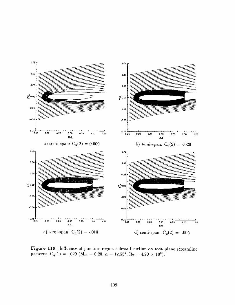
0.25 I
ooo C>
-025
-0.50
-0.75-0.25 0.00 0.25 0.50 0.75 1.00 1.25
X/L
a) semi-span: Cq(2) = 0.000
0.75
0,50
0.25
-0.50
-0.75 .... I .... i .... I .... I .... _ , , . = I-0.25 0.00 0.25 0,50 0.75 1.00 1.25
X/L
c) semi-span: Cq(2) =-.010
0.75
0,50
0.25
0.00
-0.25
-0.50
-0.75•0,25 0.00 0.25 0.50 0.75 1.00 1.25
X/L
b) semi-span: Cq(2) = -.020
0.75
0.50
0.25
-0.50
-0.75-0.25 0.00 0.25 0.50 0.75 1.00 1.25
X/l_
d) semi-span: Cq(2) =-.005
Figure 119: Influence of juncture region sidewall suction on root plane streamline
patterns, Cq(1) = -.O2O(Moo = O.20, a = 12.55o, Re = 4.2O x 106).
199

0.75
0.50
0.25
-0.50
.2 0.00 0.25 0.50 0,75 1.00 1.25
X/L
a) full-span
0.75
0.50
0.25
-0.75-0.25 0.00 0.25 0.50 0.75 1.00 1.25
X/L
b) semi-span: Cq = 0.000
0.75
0.50
0.25
-0.50
'-0.75-0.25 0.00 0.25 0.50 0.75 1.00 1.25
X/L
c) semi-span: Cq(1) = -.020, Cq(2) -- -.005
Figure 120: Comparison of root plane streamline patterns (Moo = 0.20, a = 12.55 °,
Re = 4.20 × 10s).
2OO
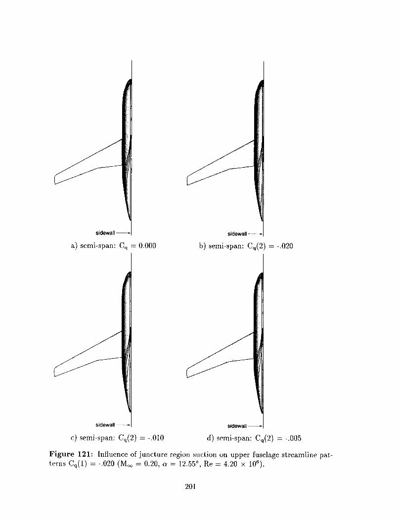
a) semi-span: Cq = 0.000
c) semi-span: Cq(2) = -.010
b) semi-span: Cq(2) =-.020
sidewall
d) semi-span: Cq(2) =-.005
Figure 121: Influence of juncture region suction on upper fuselage streamline pat-
terns Cq(1) = -.020 (Moo = 0.20, a = 12.55 °, Re = 4.20 x 10⁶).
201

C L
1.50
1.49
1.48
1.47
1.46
1.45
1.44
1,43
1.42
1.41
1.400.00
• Full-span
- - -0- - - Semi-span: Cq(2) = 0.000
.... 4X..... Semi-spa_: Cq(1) = -.020
/
/" ---0
/'" _ -0 ..... O- .......
, , , I , , , I I i i I i I
0.01 0.02 0.03
-.Cq
a) lift coefficient
0.08
C M
0.07
0.06
0.05
0.04
0.03
0.02
0.01
O.(X0.00
///
"/' - - 0
,_;__-o.....o.........
, , i i I i i I I I i I i I [
0.01 0.02 0.03
-Cq
b) pitching moment coefficient
Figure 122: Influence of sidewall suction on lift and pitching moment coefficients
(Moo = 0.20, a = 12.55 °, Re = 4.20 x 10⁶).
202

-0.50
.0.40
-0.30
ACp-o.2o
-O.10
0.00
0.10
_= .2665
1
Cq(1) = 0.000, Cq(2) = 0.000 I
......... Cq(1) = -.020, Cq(2) = 0.000 t
Cq(1) = -.020, Cq(2) = -.020 ]
i .... _ .... J .... i .... *0.00 0.25 0.50 0.75 1.00
X/C
-0.50
-0.40
..0.30
ACp.0.2o
-0.10
0.00
0.10
_=.2665
I
0.00 0.25 0.50 0.75 1.00
X/C
ACp-O.2O
-0.10
0.00
0.10
-0.50 ...................
11= .6234
-0.40 , ............
-0.30 ................
i .... i .... i .... i . . , , I
0.00 0.25 0.50 0.75 1.00
X/C
ACp.0.2o........:
-0.10
0.00
I : :010 _ .... J .... i .... J ....
0.00 0.25 0.50 0.75 1.00
X/C
-0.50 .............................................
TI= .9066
-0.40 ....
•0.30 ................... : ......
ACp-O.2O........ :
-0.10
0.00
0.10 1 .... i .... i .... i .... i
0.00 0.25 0.50 0.75 1.00
X/O
b) lower surface
Figure 123: Influence of sidewall suction on differential wing pressure distributions
(Moo =0.20, a= 12.55 °,Re=4.20 × 10⁵).
203

Cp
-1.00
-0.80
-0.60
-0.40
-0.20
0.00
0.20
0.40 -
0.60-
0.8O ;-
1.oo F0.00
'rl= 0.00
full-span
....... semi-span: Cq(1) = 0.000, Cq(2) = 0.000
..... semi-span: Cq(1) = -.020, Cq(2) = 0.000
semi-span: Cq(1) = -.020, Cq(2) = -.020
w,rootI I I = I , , , , I .... t .... I
0.25 0.50 0.75 1.00
X/L
Figure 124: Influence of sidewall suction on fuselage centerline pressure distribution
(Moo = 0.20, a = 12.55 °, Re = 4.20 × 10°).
204

071 0!.75!0.50
0.25
0.00
-11.50
-0.75 -0.75 .... i , , , , J .... I . , , , I .... J ' . J , I•0.25 0.00 0.25 0.50 0.75 1.00 1.25 -0.25 0.00 0.25 0.50 0.75 1.00 1.25
X/L X/I_
a) full-span b) semispan: Cq = 0.000
0.75
0.50
0.25
-0.75-0.25 0.00 0.25 0.50 0.75 1.00 1.25
X/L
c) semi-span: Cq(1) = -.020, Cq(2) :-.005
Figure 125: Comparison of root plane streamline patterns (Moo = 0.20 , a = 18.25 °,Re = 4.20 × 10⁶).
2O5

a) full-span b) semi-span: Cq = 0.000
c) semi-span: Cq(1) =-.020, Cq(2) =-.005
Figure 126: Influence of sidewall suction on wing upper surface streamline patterns
(Moo = 0.20, a = 18.25 °, Re = 4.20 × 10⁶).
206

-0.50i ...... 11= 12665 :
-o• I :l-0.4ql " Cq = 0.000
- Cq(1) = -.020, C (2) = -.005
ACp°-2°_I,,
-0.10 f _"-,"
0.00 _-[ _ .... ---
I0.10 i .... i .... i .... n .... i
0.00 0.25 0.50 0.75 1.00X/C
-0.50 ..................
-0.40
-0.30 .......................
A" _.2o_.,p-
11!= '2665
"0"10 I
O.OOI.L : i ...... ;= : ;j
010" • ......... i .... i
0.00 0.25 0.50 0.75 1O0
X/C
-0.50
-0.4(
-0.3,
_Cpo.2o-0.10
O.OG
0.100.00
H,
0.25 0.50 0.75 1.00
X/C
-030
ACp-0.2o
-0.10
-0.50 ;- ........... .......... .................11= .6234
:t-0.40
o.oo ____;=_.____.... i J_I
: q
0.10 J .... i .... , .... i .... ,0.00 0.25 0.50 0.75 1.00
X/C
-0.50 ..... : ...... :.....11= .9066
-0.40 ...... .... ..... .........
-0.30 : ........... .......
ACp-O.2O-0.1(:]
0.00
0.10
.... i .......
I _ 1
0.00 0.25' , , , I , , , , I , , , i I
0.50 0.75 1.00WC
a) upper surface
-0.50 - ........ :....... : ......... , ..........11=.9066
-0.40 • ............. ................ ...........
-0.30 ................. ......... : ...................
ACp-0.2o
-0.10
0.00
0.100.00
i . . . . i = , . . i . , , .
0.25 0.50
X/Cb) lower surface
• ' , , I
0.75 1.00
Figure 127: Influence of sidewall suction on differential wing pressure distributions
(Moo = 0.20, a = 18.25 °, Re = 4.20 x 10⁶).
207

-1.00
-0.80
-0.60
-0.40
-0.20
Cp o.oo
0.20
0.40
0.60
0.80
1.00
q =0.00
Full-span
....... Semi-span: Cq = 0.000
..... Semi-span: Cq(1) = -.020, Cq(2) = -.005
_" I
L wing root
!
1.00
, I _ , , , I , , , , I .... I
0.25 0.50 0.75 1.00
X/L
Figure 128: Influence of sidewall suction on fuselage centerline pressure distribution
(Moo = 0.20, c_ = 18.25 °, Re = 4.20 x 10⁶).
208

tunnel sidewall
non-metric
stand-off
metric
semi-span
rno_
a) non-metric stand-off
metric
stand-off
metric
semi-span
model
b) metric stand-off
Figure 129: Comparison of semi-span model mounting techniques.
209

0.25
C M 0.00
-0.25 I t I
C L
2.00
1.50
1.00
0.50
0.000.0
--o-_ non-metric stand-off
metric stand-off
- - - •- - - metric stand-off + correction
5.0 102 15.0 20.0
deg.
Figure 130: Demonstration of metric stand-off correction procedure (Moo = 0.20,
Re = 4.20 × 10⁶).
210

-1.00
-0.80
-0.60
-0.40
-0.20
Cp o.oo
0.20
0.40
0.60
0.80
1.00
root
...... tip
0.00 0.25 0.50 0.75 1.00
X/L
Figure 131: Comparison of computed stand-off pressure distributions (Moo = 0.20,
c_ = 12.55 °, Re = 4.20 x 10⁶).
211

y=h/2
TLNS3D (209 pts.)
• 100 pts.
-0.60
Cp
-0.40 -
-0.20 -
0.00 -
0.20 -
0.40 -
0.60 -
0.80 -
1.00 I , , , = I = _ n _ I = J = _ I .... I
0.00 0.25 0.50 0.75 1.00
X/L
Figure 132: Proposed pressure tap distribution on metric stand-off.
212

blowing jot
or slot
/
thigh pressure air
a) actual blowing jet
Block 1
I
_ grid block boundary
Block 2
b) simulated blowing jet
Figure 133: Comparison of actual and simulated tangential blowing jets.
213

"_(i- 1,j=2) / (i,_2)
I 0I
I (i,j=l)
ghost cell
(i+1 ,j=3) lo j
(i+1 ,j=2)0
t
I
I
I
[
I
I
i___,,.
simulatedporous
surface
Figure 134: Nomenclature for porous surface boundary condition.
214

0.020
0.015
'_ 0.010
0.005
0.0000.0(
o
TLNS3D
theory (Blasius)
0.25 0.50 0.75 1,00
u/U
Figure 135: Comparison of computed and theoretical laminar flat plate velocity
profiles (Rex -- 0.50 x ]06,Cq : 0.000).
215

0.020
0.015
1] 0.010
0.005
TLNS3D
o theory
0.0000.00 0.25 0.50 0.75 1.00
u/Uo
Figure 136: Comparison of computed and theoretical laminar flat plate velocity
profile (Rex = 0.50 × 10⁶,Cq = -.010).
216

Y
1.25
0.00
-0.25
0.00 0.50 1.00 1.50
X
Figure 137: Partial view of backward facing sinusoidal ramp grid.
217

1.25 1
Y 0.50
0,25
0.00
1.25
1.00
0.75
Y o5o --
0.25
-0,25 i I -0.250.00 0.50 1.00 1.50 0,00
X
a) Cq = 0.000
------- poroLm
I • . • I I
0.50 1.00 1.50
X
b) C a = -.005
1.25
1.00
0.75
Y 0.50
0.25
0,00
-0.250,00
t--- ros I i , , , I I
0,50 1.00 1.50
X
c) Cq =-.010
Figure 138: Influence of suction on backward facing sinusoidal ramp flow
(Moo = 0.20, Re/g = 2.00 × 10⁶).
218


FormApprovedREPORT DOCUMENTATION PAGE OMB No. 0704-0188
Public reporting burden for this colleofJonOf INormmtion a, asUnlsled 1oaverage 1 hour pet response, including the time for reviewing instnJOtionL imacclliog existing data sourcelkga_e¢lng and maintaining the data needed, and o=,rnplellngimd reviewing the ¢oite¢tion of infownatlon. Send comments regarding this b_den astlmate or any nther aspect of thisoolkmtkm of information, including suggestions for reducing this burden, to Washington Headquadem Services, Directorate for Information Operatioml snd Repods, 1215 JM/erlon DavisHighway, Suite 1204, Arlington, VA 22202-4302, and to the Office Of Management and Budget, Paperwork Reduction Project (0704-0188), Washington, OC 20603.
1. AGENCY USE ONLY (Leave blank) 2. REPORT DATE 3. AEPO_T TYPE AND DATES COVERED
March 1996 Contractor Report
=4. TITLE AND SUBTITLE 5. FUNDING NUMBERS
Computational Analysis of Semi-span Model Test Techniques NCC1-169
s. AUTHONS)
Wiliam E. Milholen II; Ndaona Chokani
7. PERFORMINGORGAI_IZA'rlONNAME(S)ANDADORESS(ES)
North Carolina State University
Department of Mechanical and Aerospace Engineering
Raleigh, NC 27695-7910
9. SPONSORINGI MONITORINGAGENCYNAME(S)ANDADDRESS(ES)
National Aeronautics and Space Administration
Langley Research CenterHampton, VA 23681-0001
WU 505-59-85-01
8. PEFIFORMING ORGANIZATION
REPORT NUMBER
10. SPONSORING/MONITORiNGAGENCY REPORT NUMBER
NASA CR-4709
11. SUPPLEMENTARY NOTES
The information presented in this report was offered in partial fulfillment of the requirements for the first authorsDoctor of Philosophy Degree, NCSU, Raleigh NC, 1995. Langley Technical Monitor: L.E. Putnam
12a. DISTRIBUTION I AVAILABILITY STATEMENT 12b. DISTRIBUTION CODE
Unclassified - Unlimited
Subject Category 02
'13.ABSTRACT(Maximum200words)
A computational investigation was conducted to support the development of a semi-span model testcapability in the NASA LaRC's National Transonic Facility. This capability is required for the testing of high-lift
systems at flight Reynolds numbers. A three-dimensional Navier-Stokes solver was used to compute thelow-speed flow over both a full-span configuration and a semi-span configuration. The COmputational resultswere found to be in good agreement with the experimental data. The computational results indicate that the
stand-off height has a strong influence on the flow over a semi-span model. The semi-span model adequately
replicates the aerodyamic characteristics of the full-span configuration when a small stand-off height,approximately twice the tunnel empty sidewall boundary layer displacement thickness, is used. Several activesidewall boundary layer control techniques were examined including: upstream blowing, local jet blowing, andsidewall suction. Both upstream tangential blowing, and sidewall suction were found to minimize the separationof the sidewall boundary layer ahead of the semi-span model. The required mass flow rates are found to be
practicable for testing in the NTF. For the configuration examined, the active sidewall boundary layer controltechniques were found to be necessary only near the maximum lift conditions.
14. SUBJECT TERMS
semi-span model, Navier-Stokes solutions, stand-off height, metric stand-off, local
blowing jets, upstream blowing slot, sidewall suction, National Transonic Facility
17. SECURITY CLASSIFICATIONOF REPORT
unclassified
18. SECURITY CLASSIFICATIONOF THIS PAGE
unclassified
NSN 7540-01-280-5500
19. SECURITY CLASSIFICATION
OF ABSTRACT
unclassified
i15. NUMBER OFPAGES
227
16. PRICE CODE
All
20. LIMITATION OF ABSTRACT
Standard Form 298 (Rev. 2-89)Prelcribed by ANSI Std. Z39-18298-102