Embed Size (px)
Citation preview

Computational Analysis of Flow Cytometry Datausing R / Bioconductor
BioC 2011
Greg Finak1
1Fred Hutchinson Cancer Research Center
July 29, 2011
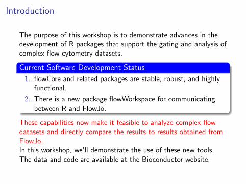
Introduction
The purpose of this workshop is to demonstrate advances in thedevelopment of R packages that support the gating and analysis ofcomplex flow cytometry datasets.
Current Software Development Status
1. flowCore and related packages are stable, robust, and highlyfunctional.
2. There is a new package flowWorkspace for communicatingbetween R and FlowJo.
These capabilities now make it feasible to analyze complex flowdatasets and directly compare the results to results obtained fromFlowJo.In this workshop, we’ll demonstrate the use of these new tools.The data and code are available at the Bioconductor website.

The Importance of the R/FlowJo Dialog
R and FlowJo provide two different, equally important roles dataanalysis.
Benefits of Collaboration
1. FlowJo enables the cytometrist to develop an analysis thatcaptures biological meaning.
2. R enables the use of modern machine learning methods andobjective, numerical approaches.
3. The informatician needs to understand what the cytometristdid to ensure the correct methods are used.
4. The cytometrist needs to review and validate the results ofthe R analysis.
The new possibilities for collaboration will increase theeffectiveness of both approaches.
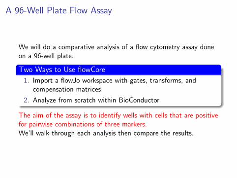
A 96-Well Plate Flow Assay
We will do a comparative analysis of a flow cytometry assay doneon a 96-well plate.
Two Ways to Use flowCore
1. Import a flowJo workspace with gates, transforms, andcompensation matrices
2. Analyze from scratch within BioConductor
The aim of the assay is to identify wells with cells that are positivefor pairwise combinations of three markers.We’ll walk through each analysis then compare the results.
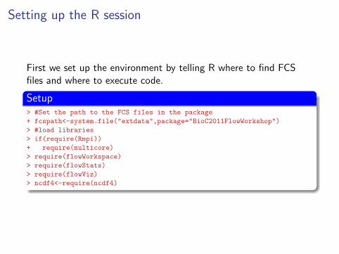
Setting up the R session
First we set up the environment by telling R where to find FCSfiles and where to execute code.
Setup> #Set the path to the FCS files in the package
+ fcspath<-system.file("extdata",package="BioC2011FlowWorkshop")
> #load libraries
> if(require(Rmpi))
+ require(multicore)
> require(flowWorkspace)
> require(flowStats)
> require(flowViz)
> ncdf4<-require(ncdf4)
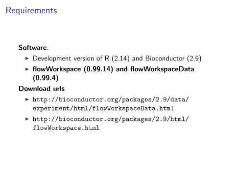
Requirements
Software:
I Development version of R (2.14) and Bioconductor (2.9)
I flowWorkspace (0.99.14) and flowWorkspaceData(0.99.4)
Download urls
I http://bioconductor.org/packages/2.9/data/
experiment/html/flowWorkspaceData.html
I http://bioconductor.org/packages/2.9/html/
flowWorkspace.html
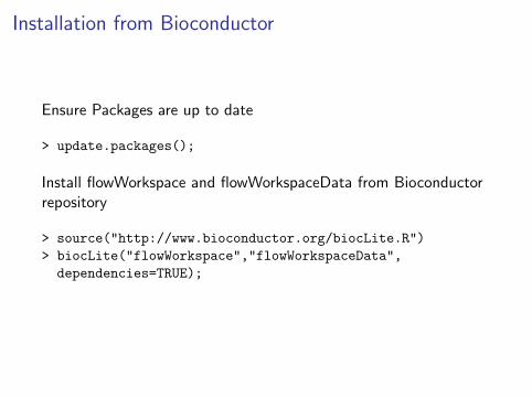
Installation from Bioconductor
Ensure Packages are up to date
> update.packages();
Install flowWorkspace and flowWorkspaceData from Bioconductorrepository
> source("http://www.bioconductor.org/biocLite.R")
> biocLite("flowWorkspace","flowWorkspaceData",
dependencies=TRUE);
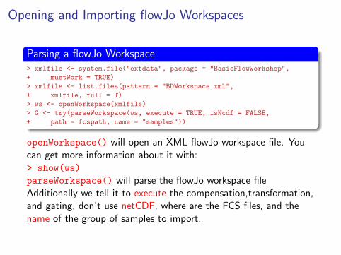
Opening and Importing flowJo Workspaces
Parsing a flowJo Workspace> xmlfile <- system.file("extdata", package = "BasicFlowWorkshop",
+ mustWork = TRUE)
> xmlfile <- list.files(pattern = "BDWorkspace.xml",
+ xmlfile, full = T)
> ws <- openWorkspace(xmlfile)
> G <- try(parseWorkspace(ws, execute = TRUE, isNcdf = FALSE,
+ path = fcspath, name = "samples"))
openWorkspace() will open an XML flowJo workspace file. Youcan get more information about it with:> show(ws)
parseWorkspace() will parse the flowJo workspace fileAdditionally we tell it to execute the compensation,transformation,and gating, don’t use netCDF, where are the FCS files, and thename of the group of samples to import.
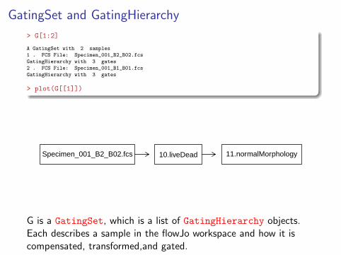
GatingSet and GatingHierarchy
> G[1:2]
A GatingSet with 2 samples
1 . FCS File: Specimen_001_B2_B02.fcs
GatingHierarchy with 3 gates
2 . FCS File: Specimen_001_B1_B01.fcs
GatingHierarchy with 3 gates
> plot(G[[1]])
Specimen_001_B2_B02.fcs 10.liveDead 11.normalMorphology
G is a GatingSet, which is a list of GatingHierarchy objects.Each describes a sample in the flowJo workspace and how it iscompensated, transformed,and gated.
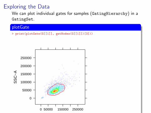
Exploring the DataWe can plot individual gates for samples (GatingHierarchy) in aGatingSet.
plotGate> print(plotGate(G[[1]], getNodes(G[[1]])[3]))
FSC−A
SS
C−
A
0
50000
100000
150000
200000
250000
0 50000 150000 250000
Plotting gates is as simple as calling plotGate with theGatingHierarchy and the gate name.Gate names can be accessed using getNodes() with theGatingHierarchy.
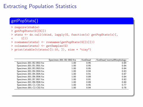
Extracting Population Statistics
getPopStats()> require(xtable)
> getPopStats(G[[5]])
> stats <- do.call(cbind, lapply(G, function(x) getPopStats(x)[,
+ 1]))
> rownames(stats) <- rownames(getPopStats(G[[1]]))
> colnames(stats) <- getSamples(G)
> print(xtable(t(stats)[1:10, ]), size = "tiny")
Specimen 001 B2 B02.fcs /liveDead /liveDead/normalMorphologySpecimen 001 B2 B02.fcs 1.00 0.95 0.84Specimen 001 B1 B01.fcs 1.00 0.95 0.84Specimen 001 B3 B03.fcs 1.00 0.95 0.84Specimen 001 B4 B04.fcs 1.00 0.94 0.83Specimen 001 B5 B05.fcs 1.00 0.91 0.87Specimen 001 B6 B06.fcs 1.00 0.89 0.84Specimen 001 B7 B07.fcs 1.00 0.91 0.82Specimen 001 B8 B08.fcs 1.00 0.89 0.80Specimen 001 C1 C01.fcs 1.00 0.95 0.77Specimen 001 C2 C02.fcs 1.00 0.94 0.78
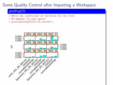
Some Quality Control after Importing a Workspace
plotPopCV> #Plot the coefficient of variation for the first
> #9 samples (to save space)
+ print(plotPopCV(G[1:9],rot=45));
cv
0.0000.0020.004
Specim
en_0
01_B
2_B02
.fcs
liveD
ead
norm
alMor
pholo
gy
Specimen_001_B1_B01.fcs
Specim
en_0
01_B
2_B02
.fcs
liveD
ead
norm
alMor
pholo
gy
Specimen_001_B2_B02.fcs
Specim
en_0
01_B
2_B02
.fcs
liveD
ead
norm
alMor
pholo
gy
Specimen_001_B3_B03.fcs
Specimen_001_B4_B04.fcsSpecimen_001_B5_B05.fcs
0.0000.0020.004
Specimen_001_B6_B06.fcs0.0000.0020.004
Specimen_001_B7_B07.fcsSpecimen_001_B8_B08.fcsSpecimen_001_C1_C01.fcs
We can to do some QC by calculating and plotting the coefficientof variation between the flowJo counts and flowCore countscomputed following import.
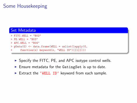
Some Housekeeping
Set Metadata> FITC.WELL = "B02"
> PE.WELL = "B03"
> APC.WELL = "B04"
> pData(G) <- data.frame(WELL = unlist(lapply(G,
+ function(x) keyword(x, "WELL ID")[[1]])))
I Specify the FITC, PE, and APC isotype control wells.
I Ensure metadata for the GatingSet is up to date.
I Extract the ‘WELL ID‘ keyword from each sample.
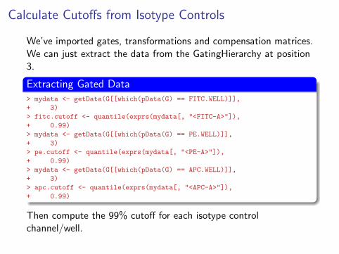
Calculate Cutoffs from Isotype Controls
We’ve imported gates, transformations and compensation matrices.We can just extract the data from the GatingHierarchy at position3.
Extracting Gated Data> mydata <- getData(G[[which(pData(G) == FITC.WELL)]],
+ 3)
> fitc.cutoff <- quantile(exprs(mydata[, "<FITC-A>"]),
+ 0.99)
> mydata <- getData(G[[which(pData(G) == PE.WELL)]],
+ 3)
> pe.cutoff <- quantile(exprs(mydata[, "<PE-A>"]),
+ 0.99)
> mydata <- getData(G[[which(pData(G) == APC.WELL)]],
+ 3)
> apc.cutoff <- quantile(exprs(mydata[, "<APC-A>"]),
+ 0.99)
Then compute the 99% cutoff for each isotype controlchannel/well.
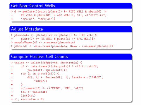
Get Non–Control Wells> d <- getData(G[which(pData(G) != FITC.WELL & pData(G) !=
+ PE.WELL & pData(G) != APC.WELL)], 3)[, c("<FITC-A>",
+ "<PE-A>", "<APC-A>")]
Adjust Metadata> phenodata <- pData(G[which(pData(G) != FITC.WELL &
+ pData(G) != PE.WELL & pData(G) != APC.WELL)])
> sampleNames(d) <- rownames(phenodata)
> pData(d) <- data.frame(phenodata, Name = rownames(pData(d)))
Compute Positive Cell Counts> tables <- unlist(fsApply(d, function(x) {
+ df <- data.frame(t(t(exprs(x)) > c(fitc.cutoff,
+ pe.cutoff, apc.cutoff)))
+ for (i in 1:ncol(df)) {
+ df[, i] <- factor(df[, i], levels = c("FALSE",
+ "TRUE"))
+ }
+ colnames(df) <- c("FITC", "PE", "APC")
+ tbl <- table(df)
+ list(tbl)
+ }), recursive = F)
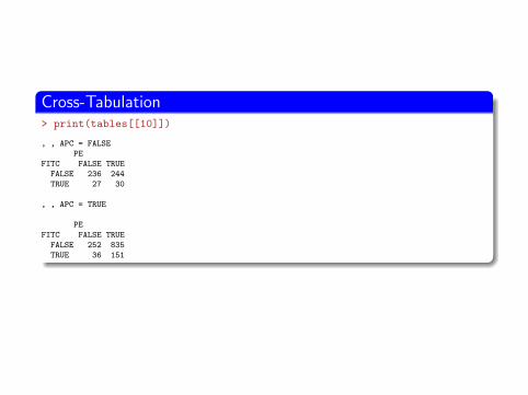
Cross-Tabulation> print(tables[[10]])
, , APC = FALSE
PE
FITC FALSE TRUE
FALSE 236 244
TRUE 27 30
, , APC = TRUE
PE
FITC FALSE TRUE
FALSE 252 835
TRUE 36 151
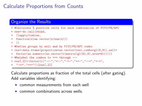
Calculate Proportions from Counts
Organize the Results> #Calculate % positive cells for each combination of FITC/PE/APC
+ res<-do.call(rbind,
+ (lapply(tables,
+ function(x)as.vector(x/sum(x)))
+ ))
> #Define groups by well and by FITC/PE/APC combo
> res<-data.frame(proportion=as.vector(res),combo=gl(8,81),well=
+ factor(as.numeric(as.vector(t(matrix(gl(81,8),nrow=8))))))
> #Relabel the combos to +++ through ---
> res[,2]<-factor(c("---","+--","-+-","++-","--+","+-+",
+ "-++","+++"))[res[,2]]
Calculate proportions as fraction of the total cells (after gating).Add variables identifying:
I common measurements from each well
I common combinations across wells.
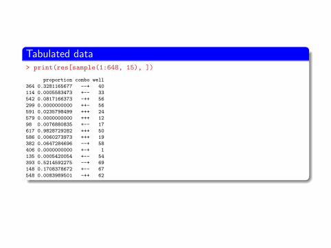
Tabulated data> print(res[sample(1:648, 15), ])
proportion combo well
364 0.3281165677 --+ 40
114 0.0005583473 +-- 33
542 0.0817166373 -++ 56
299 0.0000000000 ++- 56
591 0.0235798499 +++ 24
579 0.0000000000 +++ 12
98 0.0076880835 +-- 17
617 0.9828729282 +++ 50
586 0.0060273973 +++ 19
382 0.0647284696 --+ 58
406 0.0000000000 +-+ 1
135 0.0005420054 +-- 54
393 0.5214592275 --+ 69
148 0.1708378672 +-- 67
548 0.0083989501 -++ 62
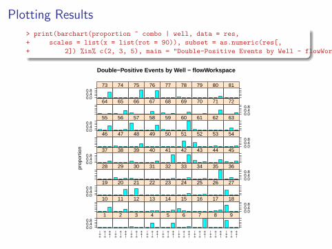
Plotting Results
> print(barchart(proportion ~ combo | well, data = res,
+ scales = list(x = list(rot = 90)), subset = as.numeric(res[,
+ 2]) %in% c(2, 3, 5), main = "Double-Positive Events by Well - flowWorkspace"))
Double−Positive Events by Well − flowWorkspacepr
opor
tion
0.00.40.8
++
−+
−+
−+
+
1
++
−+
−+
−+
+
2
++
−+
−+
−+
+
3
++
−+
−+
−+
+
4
++
−+
−+
−+
+
5
++
−+
−+
−+
+
6
++
−+
−+
−+
+
7+
+−
+−
+−
++
8
++
−+
−+
−+
+
9
10 11 12 13 14 15 16 17
0.00.40.8
180.00.40.8
19 20 21 22 23 24 25 26 27
28 29 30 31 32 33 34 35
0.00.40.8
360.00.40.8
37 38 39 40 41 42 43 44 45
46 47 48 49 50 51 52 53
0.00.40.8
540.00.40.8
55 56 57 58 59 60 61 62 63
64 65 66 67 68 69 70 71
0.00.40.8
720.00.40.8
73 74 75 76 77 78 79 80 81
That Was Easy..
Because we imported the workspace from flowJo we had little todo in the way of gating or other data pre-processing.Now let’s repeat the analysis but do the compensation and gatingin flowCore.
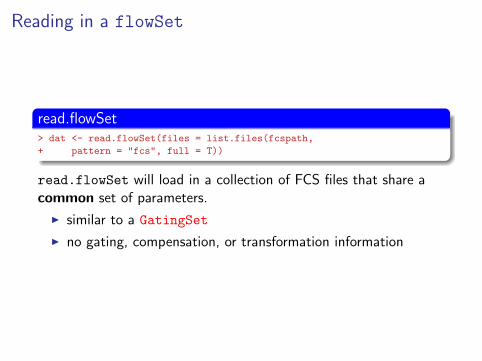
Reading in a flowSet
read.flowSet> dat <- read.flowSet(files = list.files(fcspath,
+ pattern = "fcs", full = T))
read.flowSet will load in a collection of FCS files that share acommon set of parameters.
I similar to a GatingSet
I no gating, compensation, or transformation information
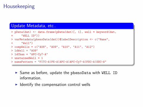
Housekeeping
Update Metadata, etc..> pData(dat) <- data.frame(pData(dat)[, 1], well = keyword(dat,
+ "WELL ID"))
> varMetadata(phenoData(dat))$labelDescription <- c("Name",
+ "Well")
> compWells = c("A08", "A09", "A10", "A11", "A12")
> ldWell = "A09"
> ldChan = "APC-Cy7-A"
> unstainedWell = 1
> namePattern = "FITC-A|PE-A|APC-A|APC-Cy7-A|FSC-A|SSC-A"
I Same as before, update the phenoData with WELL ID
information.
I Identify the compensation control wells
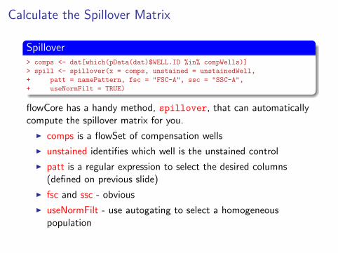
Calculate the Spillover Matrix
Spillover> comps <- dat[which(pData(dat)$WELL.ID %in% compWells)]
> spill <- spillover(x = comps, unstained = unstainedWell,
+ patt = namePattern, fsc = "FSC-A", ssc = "SSC-A",
+ useNormFilt = TRUE)
flowCore has a handy method, spillover, that can automaticallycompute the spillover matrix for you.
I comps is a flowSet of compensation wells
I unstained identifies which well is the unstained control
I patt is a regular expression to select the desired columns(defined on previous slide)
I fsc and ssc - obvious
I useNormFilt - use autogating to select a homogeneouspopulation
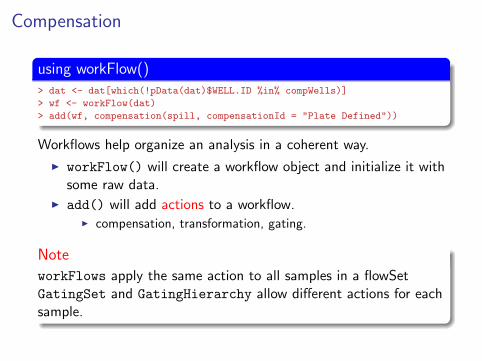
Compensation
using workFlow()> dat <- dat[which(!pData(dat)$WELL.ID %in% compWells)]
> wf <- workFlow(dat)
> add(wf, compensation(spill, compensationId = "Plate Defined"))
Workflows help organize an analysis in a coherent way.
I workFlow() will create a workflow object and initialize it withsome raw data.
I add() will add actions to a workflow.I compensation, transformation, gating.
Note
workFlows apply the same action to all samples in a flowSetGatingSet and GatingHierarchy allow different actions for eachsample.
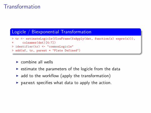
Transformation
Logicle / Biexponential Transformation> tr <- estimateLogicle(flowFrame(fsApply(dat, function(x) exprs(x))),
+ colnames(dat)[4:7])
> identifier(tr) <- "commonLogicle"
> add(wf, tr, parent = "Plate Defined")
I combine all wells
I estimate the parameters of the logicle from the data
I add to the workflow (apply the transformation)
I parent specifies what data to apply the action.
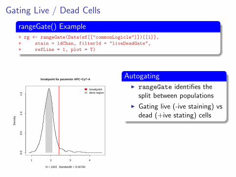
Gating Live / Dead Cells
rangeGate() Example> rg <- rangeGate(Data(wf[["commonLogicle"]])[[1]],
+ stain = ldChan, filterId = "liveDeadGate",
+ refLine = 1, plot = T)
1 2 3 4
0.0
0.5
1.0
1.5
breakpoint for parameter APC−Cy7−A
N = 2403 Bandwidth = 0.04784
Den
sity
breakpointdens region
AutogatingI rangeGate identifies the
split between populations
I Gating live (-ive staining) vsdead (+ive stating) cells
Gating Live / Dead Cells
Gate the workFlow> rg <- rangeGate(Data(wf[["commonLogicle"]]), stain = ldChan,
+ filterId = "liveDeadGate", refLine = 1)
> add(wf, rg, parent = "commonLogicle")
I Define a rangeGate on the flowSet
I Add it to the workflow (parent="commonLogicle")
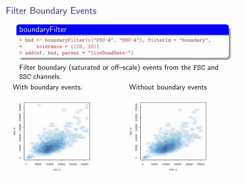
Filter Boundary Events
boundaryFilter> bnd <- boundaryFilter(c("FSC-A", "SSC-A"), filterId = "boundary",
+ tolerance = c(10, 10))
> add(wf, bnd, parent = "liveDeadGate-")
Filter boundary (saturated or off–scale) events from the FSC andSSC channels.
With boundary events.
0 50000 100000 150000 200000 250000
050
000
1000
0015
0000
2000
0025
0000
FSC−A
SS
C−
A
Without boundary events
0 50000 100000 150000 200000 250000
050
000
1000
0015
0000
2000
0025
0000
FSC−A
SS
C−
A
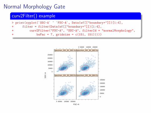
Normal Morphology Gate
curv2Filter() example> print(xyplot(`SSC-A` ~ `FSC-A`, Data(wf[["boundary+"]])[1:4],
+ filter = filter(Data(wf[["boundary+"]])[1:4],
+ curv2Filter("FSC-A", "SSC-A", filterId = "normalMorphology",
+ bwFac = 7, gridsize = c(151, 151)))))
FSC−A
SS
C−
A
0
50000
100000
150000
200000
250000
Specimen_001_B1_B01.fcs
0 50000 150000 250000
Specimen_001_B2_B02.fcs
0 50000 150000 250000
Specimen_001_B3_B03.fcs
0
50000
100000
150000
200000
250000
Specimen_001_B4_B04.fcs
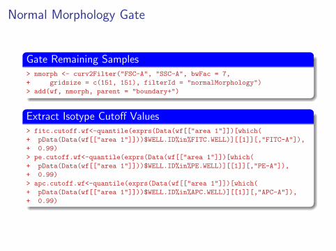
Normal Morphology Gate
Gate Remaining Samples> nmorph <- curv2Filter("FSC-A", "SSC-A", bwFac = 7,
+ gridsize = c(151, 151), filterId = "normalMorphology")
> add(wf, nmorph, parent = "boundary+")
Extract Isotype Cutoff Values> fitc.cutoff.wf<-quantile(exprs(Data(wf[["area 1"]])[which(
+ pData(Data(wf[["area 1"]]))$WELL.ID%in%FITC.WELL)][[1]][,"FITC-A"]),
+ 0.99)
> pe.cutoff.wf<-quantile(exprs(Data(wf[["area 1"]])[which(
+ pData(Data(wf[["area 1"]]))$WELL.ID%in%PE.WELL)][[1]][,"PE-A"]),
+ 0.99)
> apc.cutoff.wf<-quantile(exprs(Data(wf[["area 1"]])[which(
+ pData(Data(wf[["area 1"]]))$WELL.ID%in%APC.WELL)][[1]][,"APC-A"]),
+ 0.99)
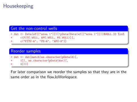
Housekeeping
Get the non-control wells> dat <- Data(wf[["area 1"]])[!pData(Data(wf[["area 1"]]))$WELL.ID %in%
+ c(FITC.WELL, APC.WELL, PE.WELL)][,
+ c("FITC-A", "PE-A", "APC-A")]
Reorder samples> dat <- dat[match(as.character(pData(d)[,
+ 1]), as.character(pData(dat)[,
+ 2]))]
For later comparison we reorder the samples so that they are in thesame order as in the flowJoWorkspace.
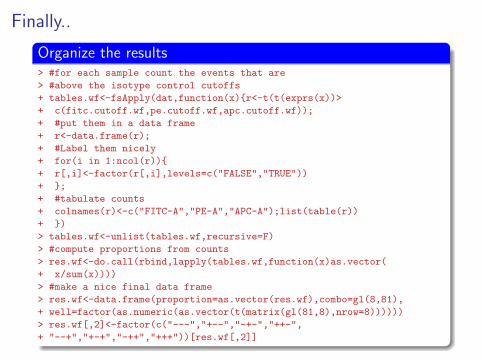
Finally..
Organize the results> #for each sample count the events that are
> #above the isotype control cutoffs
+ tables.wf<-fsApply(dat,function(x){r<-t(t(exprs(x))>
+ c(fitc.cutoff.wf,pe.cutoff.wf,apc.cutoff.wf));
+ #put them in a data frame
+ r<-data.frame(r);
+ #Label them nicely
+ for(i in 1:ncol(r)){
+ r[,i]<-factor(r[,i],levels=c("FALSE","TRUE"))
+ };
+ #tabulate counts
+ colnames(r)<-c("FITC-A","PE-A","APC-A");list(table(r))
+ })
> tables.wf<-unlist(tables.wf,recursive=F)
> #compute proportions from counts
> res.wf<-do.call(rbind,lapply(tables.wf,function(x)as.vector(
+ x/sum(x))))
> #make a nice final data frame
> res.wf<-data.frame(proportion=as.vector(res.wf),combo=gl(8,81),
+ well=factor(as.numeric(as.vector(t(matrix(gl(81,8),nrow=8))))))
> res.wf[,2]<-factor(c("---","+--","-+-","++-",
+ "--+","+-+","-++","+++"))[res.wf[,2]]
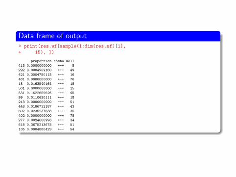
Data frame of output> print(res.wf[sample(1:dim(res.wf)[1],
+ 15), ])
proportion combo well
413 0.0000000000 +-+ 8
292 0.0004909180 ++- 49
421 0.0004780115 +-+ 16
481 0.0000000000 +-+ 76
18 0.0163540164 --- 18
501 0.0000000000 -++ 15
531 0.1622659626 -++ 45
99 0.0110630111 +-- 18
213 0.0000000000 -+- 51
448 0.0186732187 +-+ 43
602 0.0235237638 +++ 35
402 0.0000000000 --+ 78
277 0.0024666996 ++- 34
618 0.3675213675 +++ 51
135 0.0004880429 +-- 54
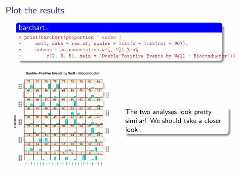
Plot the results
barchart..> print(barchart(proportion ~ combo |
+ well, data = res.wf, scales = list(x = list(rot = 90)),
+ subset = as.numeric(res.wf[, 2]) %in%
+ c(2, 3, 5), main = "Double-Positive Events by Well - Bioconductor"))
Double−Positive Events by Well − Bioconductor
prop
ortio
n
0.00.40.8
++
−+
−+
−+
+
1
++
−+
−+
−+
+
2
++
−+
−+
−+
+
3
++
−+
−+
−+
+
4
++
−+
−+
−+
+
5
++
−+
−+
−+
+
6
++
−+
−+
−+
+
7
++
−+
−+
−+
+
8
++
−+
−+
−+
+
9
10 11 12 13 14 15 16 17
0.00.40.8
180.00.40.8
19 20 21 22 23 24 25 26 27
28 29 30 31 32 33 34 35
0.00.40.8
360.00.40.8
37 38 39 40 41 42 43 44 45
46 47 48 49 50 51 52 53
0.00.40.8
540.00.40.8
55 56 57 58 59 60 61 62 63
64 65 66 67 68 69 70 71
0.00.40.8
720.00.40.8
73 74 75 76 77 78 79 80 81
The two analyses look prettysimilar! We should take a closerlook..
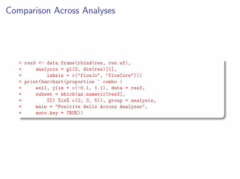
Comparison Across Analyses
> res3 <- data.frame(rbind(res, res.wf),
+ analysis = gl(2, dim(res)[1],
+ labels = c("flowJo", "flowCore")))
> print(barchart(proportion ~ combo |
+ well, ylim = c(-0.1, 1.1), data = res3,
+ subset = which(as.numeric(res3[,
+ 2]) %in% c(2, 3, 5)), group = analysis,
+ main = "Positive Wells Across Analyses",
+ auto.key = TRUE))
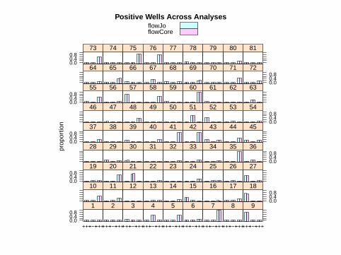
Positive Wells Across Analyses
prop
ortio
n
0.00.40.8
++−+−+−++
1
++−+−+−++
2
++−+−+−++
3
++−+−+−++
4
++−+−+−++
5
++−+−+−++
6
++−+−+−++
7
++−+−+−++
8
++−+−+−++
9
10 11 12 13 14 15 16 17
0.00.40.8
180.00.40.8
19 20 21 22 23 24 25 26 27
28 29 30 31 32 33 34 35
0.00.40.8
360.00.40.8
37 38 39 40 41 42 43 44 45
46 47 48 49 50 51 52 53
0.00.40.8
540.00.40.8
55 56 57 58 59 60 61 62 63
64 65 66 67 68 69 70 71
0.00.40.8
720.00.40.8
73 74 75 76 77 78 79 80 81
flowJoflowCore
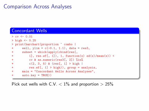
Comparison Across Analyses
Concordant Wells> cv <- 0.01
> high <- 0.25
> print(barchart(proportion ~ combo |
+ well, ylim = c(-0.1, 1.1), data = res3,
+ subset = which(apply(cbind(res[,
+ 1], res.wf[, 1]), 1, function(x) sd(x)/mean(x)) <
+ cv & as.numeric(res3[, 2]) %in%
+ c(2, 3, 5) & (res[, 1] > high |
+ res.wf[, 1] > high)), group = analysis,
+ main = "Concordant Wells Across Analyses",
+ auto.key = TRUE))
Pick out wells with C.V. < 1% and proportion > 25%
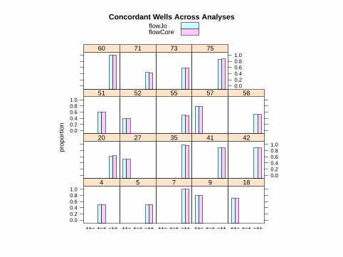
Concordant Wells Across Analyses
prop
ortio
n
0.00.20.40.60.81.0
++− +−+ −++
4
++− +−+ −++
5
++− +−+ −++
7
++− +−+ −++
9
++− +−+ −++
18
20 27 35 41
0.00.20.40.60.81.0
420.00.20.40.60.81.0
51 52 55 57 58
60 71 73
0.00.20.40.60.81.0
75
flowJoflowCore
In Conclusion
You should now have a basis (examples and working code) foranalyzing your own data.-Import preprocessing and gates from flowJo-Or (for the brave) entirely within BioConductorOther features of flowWorkspace not covered here:-NetCDF support (requires ncdf4 package and netcdf4 C library)Just pass isNCDF=TRUE to parseWorkspace()
-Parallel processing using Rmpi and multicore packages.Pass nslaves=# to parseWorkspace()
More complete netCDF support coming (ncdfFlow package).flowWorkspace constantly being improved.
Acknowledgements
rglab.org
I Raphael Gottardo
I Mike Jiang
I Mose Andre
HVTN
I Steve DeRosa
Bioconductor
I Nishant Gopalakrishnan
I Chao-Jen Wong
Funding NIH R01 EB008400 andthe ITN