Linköping Studies in Science and Technology. Theses. No. 993

Computation of Thermal Development in Injection Mould Filling,

based on the Distance Model

Per-Åke Andersson

Department of Mathematics Linköpings universitet, SE-581 83 Linköping, Sweden

Linköping 2002

Computation of Thermal Development in Injection Mould Filling, based on the Distance Model

2002 Per-Åke Andersson

Matematiska institutionen Linköpings universitet SE-581 83 Linköping, Sweden peand@mai.liu.se

LiU-TEK-LIC-2002:66 ISBN 91-7373-563-9 ISSN 0280-7971

Printed by UniTryck, Linköping 2002

iii

Contents Abstract v Acknowledgements vi

1 Introduction 1

1.1 Purpose and limitations 1 1.2 Method principles 2 1.3 Structure of the thesis 4

2 Injection moulding and temperature modelling 5

2.1 Modes of heat transfer 5 2.2 Temperature dependent material properties 6

2.2.1 Heat capacity and latent heat 6 2.2.2 Density and thermal conductivity 7 2.2.3 Viscosity 8 2.2.4 Dimensionless groups and asymptotic temperature profiles 9 2.2.5 Assumptions 10

2.3 The governing equations 11 2.3.1 General notation 11 2.3.2 Mass and momentum balance 11 2.3.3 Energy balance 13

2.4 Boundary conditions 13 2.4.1 Symmetry, points of injection and mould walls 13 2.4.2 Flow front 14

3 Model and method 15

3.1 Analytical sub-models 15 3.1.1 Vertical velocity profile 15 3.1.2 Pressure distribution 17 3.1.3 Freezing layer 18 3.1.4 Fountain flow 20

3.2 PDEs and solution method 22 3.2.1 General and regional melt PDEs 22 3.2.2 Time marching and pseudo-radial marching 25 3.2.3 Outer iteration: Surface of frozen layer 25 3.2.4 Inner iteration: Vertical temperature profile 26 3.2.5 Cooling PDE and its series solution 27 Flowchart 3.1 Data processing 30 Flowchart 3.2 Solution routine for active flow. Radial symmetry 31 Flowchart 3.3 Solution routine for passive flow 31

3.3 FD scheme 32 3.3.1 Control volume approach and truncation error 32 3.3.2 Convergence of inner iterations 37

iv

4 Application: Circular plate 41

4.1 Special modelling: Radial flow 41 4.2 Materials data 42 4.3 Comparison runs 45

4.3.1 Pressure distribution 45 4.3.2 Temperature distribution 47

4.4 Variation of physical model 53 4.4.1 Latent heat of crystallization 53 4.4.2 Heat conductivity 53 4.4.3 Viscosity dependence of pressure 53

4.5 Method performance 55 4.5.1 Relations to the number of vertical levels (control volumes) 55 4.5.2 Wall series solution 56 4.5.3 Control volume at the frozen layer 56

5 Application: Triangular plate 59

5.1 Special modelling: Geometry 59 5.2 Materials data 61 5.3 Comparison runs 63

5.3.1 Average temperature 63 5.3.2 Temperature profiles 71

5.4 Method performance 72 5.4.1 Square-root parameter 72 5.4.2 Iteration statistics 72 5.4.3 Velocity profiles and residence time 72

6 Conclusions 75

7 References 77 Appendix 1 Vertical velocity profiles 79 Appendix 2 Further comments on the Stefan problem 80

A2.1 Freezing layer in the presence of particular heat generation 80 A2.2 Initial front temperatures by the square-root model 82

Appendix 3 Solid melt: a series solution 83 Appendix 4 Comments on the PDE and its well-posedness 85 Appendix 5 Stability of linearized FD scheme 87

v

Abstract

The heat transfer in the filling phase of injection moulding is studied, based on Gunnar Aronsson’s distance model for flow expansion ([Aronsson], 1996).

The choice of a thermoplastic materials model is motivated by general physical properties, admitting temperature and pressure dependence. Two-phase, per-phase-incompressible, power-law fluids are considered. The shear rate expression takes into account pseudo-radial flow from a point inlet.

Instead of using a finite element (FEM) solver for the momentum equations a general analytical viscosity expression is used, adjusted to current axial temperature profiles and yielding expressions for axial velocity profile, pressure distribution, frozen layer expansion and special front convection.

The nonlinear energy partial differential equation is transformed into its conservative form, expressed by the internal energy, and is solved differently in the regions of streaming and stagnant flow, respectively. A finite difference (FD) scheme is chosen using control volume discretization to keep truncation errors small in the presence of non-uniform axial node spacing. Time and pseudo-radial marching is used. A local system of nonlinear FD equations is solved. In an outer iterative procedure the position of the boundary between the “solid” and “liquid” fluid cavity parts is determined. The uniqueness of the solution is claimed. In an inner iterative procedure the axial node temperatures are found. For all physically realistic material properties the convergence is proved. In particular the assumptions needed for the Newton-Mysovskii theorem are secured. The metal mould PDE is locally solved by a series expansion. For particular material properties the same technique can be applied to the “solid” fluid.

In the circular plate application, comparisons with the commercial FEM-FD program Moldflow (Mfl) are made, on two Mfl-database materials, for which model parameters are estimated/adjusted. The resulting time evolutions of pressures and temperatures are analysed, as well as the radial and axial profiles of temperature and frozen layer. The greatest differences occur at the flow front, where Mfl neglects axial heat convection. The effects of using more and more complex material models are also investigated. Our method performance is reported.

In the polygonal star-shaped plate application a geometric cavity model is developed. Comparison runs with the commercial FEM-FD program Cadmould (Cmd) are performed, on two Cmd-database materials, in an equilateral triangular mould cavity, and materials model parameters are estimated/adjusted. The resulting average temperatures at the end of filling are compared, on rays of different angular deviation from the closest corner ray and on different concentric circles, using angular and axial (cavity-halves) symmetry. The greatest differences occur in narrow flow sectors, fatal for our 2D model for a material with non-realistic viscosity model. We present some colour plots, e.g. for the residence time.

The classical square-root increase by time of the frozen layer is used for extrapolation. It may also be part of the front model in the initial collision with the cold metal mould. An extension of the model is found which describes the radial profile of the frozen layer in the circular plate application accurately also close to the inlet.

The well-posedness of the corresponding linearized problem is studied, as well as the stability of the linearized FD-scheme.

vi

Acknowledgements

I am most grateful to the Swedish Council of Science, the Department of Mathematics at Linköping University, especially my supervisor professor Gunnar Aronsson and the Section of Applied Mathematics, and the Departments of Technology and Science at Örebro University, especially the Section of Mathematics (where I am a member of staff), for their confidence by awarding me, a ”55+”, the privilege of education and research, and for financially and morally supporting me.

I respectfully acknowledge the unsponsored work performed by Mari Valtonen, Tampere University of Technology, and Lars-Åke Nilsson, PolyInvent AB, on FEM-FD simulation runs.

I express my sincere gratitude to Tommy Elfving and Gunnar Aronsson for many valuable comments on my writing.

I am much obliged to Lena.

1.1 Purpose and limitations

1 Introduction 1.1 Purpose and limitations One of the main reasons for studying temperature in injection moulding is the need for judging the risk of such local freezing that may lead to an incomplete filling of the mould cavity. The typical cavity domain is characterized by a small extension in one – gap – direction, i.e. the filling is “essentially” a 2D process.

In commercial FEM-FD (finite elements method, finite differences) programs the expansion flow and the temperature of the molten plastic are computed simultaneously.

This thesis is based upon the distance model, which asymptotically (i.e. for power-law fluids of small index values, see [Aronsson]) describes how a polymer melt expands from an injection point and fills the mould cavity, without consideration of temperatures. Our separate tempera-ture model becomes a consistency check, and may also act as a correction tool, if necessary.

The study is limited to the filling of the mould cavity. This means that the packing and cooling phases of the process are omitted, and the varying influence of the inlet and cooling channels on temperatures is ignored.

The cooling phase of the process gives the main reduction of temperatures, by 100 Co or more during several tens of seconds. The objective for considering the shorter filling phase – of magnitude 1-3 seconds – becomes e.g. to correctly identify situations where local freezing of streaming fluid exceeds some critical limit, e.g. a prescribed proportion of the mould gap at some mould positions, rather than to accurately describe the temperature distribution over the gap or even the average temperature. Temperature effects can also be crucial for warpage, poor welds (flow marks), burning, brittleness and parts flashing ([Becker et al.], p.203, and [Berins], p.161).

The flow front velocities that are generated by the distance model, combined with a simple viscosity based model, act as inputs to an energy equation; which makes the temperature computation much simpler than when coupled with the traditional Navier-Stokes equations. However, there is a need for additional assumptions:

• the local flow direction is steady,

• the pseudo-circles, that describe the flow front expansion (see [Aronsson], p.428), define isobars until local stagnation,

• the cavity parts that share flow history are equivalent as to temperature evolution.

The general aim for the temperature model and its computational method is to match the simplicity of the distance model and the fastness of the corresponding shortest route method, hopefully making a later integration possible.

For comparison purposes several materials are studied, with data easily available and chosen to reflect different properties of viscosity and latent heat.

1

1.2 Method principles

“liquid” melt

lT

TE

gap symmetry plane

Tno-flow

h

wall surface

axial gap position z

frozen surface

“solid” melt

sT

metal mould

wT

H0

cooling circuit

axial node

Figure 1.1 b Computational quantities in axial section, for given radial and angular position.

Figure 1.1 a Regions of streaming and stagnant fluid during filling. Radial flow.

The work is theoretical and no practical evaluation on real moulding data has been performed. The developed computer program is basically a numerical FD scheme, and simulation comparisons are made with two commercial FEM-FD programs.

To be strictly consistent with the assumptions of the distance model, the fluid viscosity should be independent of temperature – the isothermal case. In the standalone FD program this is a special case of a more general material model.

The FD simulations are performed on a PC computer, using C++ for computational purposes and Matlab ( The MathWorks, Inc.) for graphics.

1.2 Method principles We consider two kinds of applications: disk- and polygonal star-shaped cavities, with one “point” of injection. Our simplifying assumption is that the main flow is radial, an “essentially” 1D process, i.e. that any angular flow and heat exchange can be neglected. During the filling phase of a triangular cavity the flow situation may look like in Figure 1.1a.

2

Active-flow sector of streaming fluid

Passive-flow sub-region of stagnant fluid

Front arc

Inlet

1.2 Method principles

In Fig. 1.1a we identify three active-flow sectors (sub-regions), with one circular front arc each, and three passive-flow sub-regions. These two types of regions are handled separately:

• In the active-flow sub-regions the resulting PDE is solved by time-marching, i.e. we discretize the time from start to end of the filling phase in discrete time steps

Kk ,,1K= . For each time step k we practice radial marching in radial steps ki ,,1K= from inlet to front, i.e. we approximate the PDE by a system of FD

equations for the current temperature distribution at ),( ik . Because of the radial symmetry, all nodes that are concentrically placed relative to the inlet (common i) share flow history and are treated as one common node group. In both the disk- and polygonal star-shaped applications one ray of maximum length, i.e. an arbitrary disk ray and one polygonal corner ray, respectively, is sufficient to characterize the whole active-flow process.

• In the passive-flow sub-regions we have to distinguish more node groups, since Fig. 1.1a shows that both the radial position and the time of stagnation, i.e. when the flow hits the wall along the stream ray through the node, have to coincide to define equivalent flow history. For each node group i of common flow history we perform time-marching by steps k from the time of stagnation to the end of filling. The start temperatures of the stagnant ray in focus are received from the active-flow evolution, the snapshot taken at the time of ray stagnation (wall hit).

The solution method is the same in both types of flow regions, for every given time step k and node group i. In Figure 1.1b the basic symbols are shown. The gap-wise direction z is drawn from the centre symmetry plane 0=z to the nominal wall surface Hz = . The local effective gap width h, that separates streaming fluid from “frozen” melt, is defined by the no-flow temperature flownoT − . In each phase of state, “liquid” and “solid”, a system of nonlinear FD-equations is solved for the temperatures lT , sT at the given axial node positions jz ,

Jj ,,1,0 K= (with 20=J in Fig. 1.1b). This is made in an inner iterative procedure for fixed h, primarily by the damped Newton-Raphson method. The correct local position of h is determined in an outer iterative procedure, taking into account the heat flow between the two melt phases. The interaction with the metal mould is managed by a series expansion solution for the wall temperatures wT , reducing the computation of local heat exchange mould - cavity to a mere analytical updating. Our strategy involves solving two small systems of altogether J+1 nonlinear FD-equations many times, once for each trial h-value of each ),( ik -combination. The axial node positions are chosen to balance two conflicting aims: capturing the steep temperature change at the frozen layer and reducing the truncation errors.

3

1.3 Structure of the thesis

1.3 Structure of the thesis In Chapter 2 we describe the major elements of our temperature model for the filling phase of injection moulding – the modes of heat transfer, the relevant materials properties, and the basic model assumptions, equations and boundary conditions.

In Chapter 3 our model and method are presented, for (pseudo-)radial expansion flow. The basic energy model is extended by some analytical submodels – one replacing the absent pressure-momentum equations, one extrapolating the expansion of the frozen layer, and two variants handling the flow front energy. A numerical FD-scheme and a positioning principle for the axial nodes are derived. The general method (cf. Sec. 1.2) is fully described and its expected behaviour is analysed.

Our method is implemented for two different applications. The first type, studied in Ch. 4, is disk shaped cavities. Two commodity materials, an amorphous polycarbonate (PC) and a semi-crystalline polyethylene (HDPE) are modelled. Four comparison simulation runs of the FEM-FD-program Moldflow (of Moldflow Corp.) and our FD-program are evaluated. The influence of our more extended material models upon the resulting temperature and frozen layer profiles is studied. Some aspects of our method performance are documented.

In Ch. 5 we treat the second application type, polygonal star-shaped cavities (relative to the inlet), of constant gap width (cf. Fig. 1.1a). The special geometry modelling is described. Two commodity thermoplastics, an amorphous polystyrene (PS) and a semi-crystalline polyoxymethylene (POM), are studied. Two, out of four intended, comparison simulation runs of the FEM-FD-program Cadmould (of Simcon) and our FD-program are documented. Apart from the comparison figures, some of our internal FD-model and method results are reported, partly as colour plots. These include the calculated times of injection.

Our main conclusions are presented in Ch. 6.

In Appendices 1 – 5 some results related to the implemented routine are collected. We give examples from the assumed class of velocity profiles and the corresponding temperature profiles, derive a class of square-root solutions characterizing the expansion of the frozen layer in radial flow, present a series expansion solution for the temperatures in the frozen sub-regions, and treat the well-posedness of the linearized PDE as well as the stability of the linearized FD-scheme for given frozen layer profiles.

4

2.1 Modes of heat transfer

2 Injection moulding and temperature modelling In this chapter we describe the basic elements of our temperature model for the filling phase of injection moulding. The conductive and convective heat transfer modes are identified in Sec. 2.1. By using the practical concept of a no-flow temperature, which subdivides the fluid into an essentially immobile (“solid”, “frozen”) and a mobile (“liquid”) phase of state, we can treat both semi-crystalline thermoplastics and amorphous materials in Sec. 2.2. For the main material properties – heat capacity, latent heat of crystallization, density, heat conductivity and viscosity – we judge whether constant or simple linear or nonlinear functions of temperature and/or pressure are needed to capture the main variations. We argue that the non-asymptotic character and the dynamics of the filling process would make a model based upon dimensionless quantities, like the Cameron number, of less value. In Sec. 2.3 the underlying assumptions of the distance model, for flow expansion and pressure field, are listed. The basic equations are formulated, with focus on the energy PDE. Due to the temperature dependent fluid properties, the energy equation becomes nonlinear. A temperature dependent viscosity makes the momentum/pressure field equations depend upon the temperature solution of the energy PDE, while shear rate, convection velocity and pressure provide a link in the opposite direction. Finally in Sec. 2.4 the boundary conditions are listed. The special difficulties of the moving flow front are noticed.

2.1 Modes of heat transfer From an inlet “point” (gate) where the thermoplastic is injected into the mould cavity, the expansion of the hot polymer melt means a thermal convection that is essentially radial. In the filled cavity parts heat is transferred by conduction mainly in the gap-wise (z-)direction to the metallic walls, where cooling channels transport heat out of the mould.

Near the cavity walls streaming melt is subject to high shear rates, which tends to increase the temperature through viscous dissipation. A frozen layer of cooled, stagnant melt is built up at the walls, to some extent acting as an insulation layer between the streaming fluid and the cold walls.

Since most polymers are non-opaque to infrared light, some radiation energy hits the metallic wall surface.

In the absence of sharp cavity corners, laminar flow dominates the filling process except at the flow front, where heat is transferred straight to the walls by convection across the gap. The corresponding orientation of the polymer chains – normal at the very wall surface and tangential in the laminar zone (see, e.g., [Tadmor & Gogos], p.608) – affects conduction.

For the filling phase, the fluid properties normally identify one temperature of dramatic changes, the practical concept flownoT − . (In Sec. 2.2 it can be identified as MT or GT .)

5

2.2 Temperature dependent material properties

2.2 Temperature dependent material properties

2.2.1 Heat capacity and latent heat In a process where the material density ρ is almost fixed, the constant-pressure heat capacity

Pc nearly coincides with the constant-volume heat capacity (the difference is around 10% for polymers, see [Rao], p.37). For amorphous polymers, Pc increases continuously and slowly with increasing temperature except at a point of discontinuity – the glass transition temperature GT – where the polymer from a colder glassy state becomes more easily deformable – rubbery – and the Pc -curve has a step-up jump.

For semi-crystalline polymers, ordered crystalline regions are surrounded by a matrix of less ordered, rubbery amorphous material, making the polymer tough and leathery above GT , and brittle through a glassy amorphous matrix below GT ([Morton-Jones], p.14). At the temperature where the crystalline structure is lost, the Pc -curve shows a narrow peak, where the position of the maximum defines the melting point MT . By cooling such a material the latent heat of solidification (crystallisation) ML is released. Realistic modelling is complicated by such phenomena as sub-cooling and slow crystallisation.

For practical purposes, Pc can be considered as pressure independent ([Tadmor & Gogos], p.139).

As for the physical state of injection moulded thermoplastics at room temperature, PP, HDPE and POM are semi-crystalline between GT and MT , and PA 6 is below GT , while the materials ABS, PVC, PMMA, PC and PS are examples of amorphous polymers below GT (e.g. [Becker et al.], p.20).

When data are unavailable, [Van Krevelen], p.116 recommends the following linear, empirical expressions, referring Pc at T (in Co ) to (extrapolated) values at room temperature:

)2.2( )].25(0012.01[)C 25()()1.2( )],25(003.01[)C 25()(

,,

,,

−⋅+⋅=−⋅+⋅=

TcTcTcTc

PP

sPsPo

ll

o

Here (2.1) is valid for s = “solid” state, i.e. both semi-crystalline polymers with MTT < and amorphous thermoplastics with GTT < ; otherwise (2.2) applies – for l = “liquid” state. As an alternative, constant levels are used in the solid and liquid states, respectively. The error of such an approximation can be evaluated by (2.1) and (2.2), where the Pc -values change by 30% and 12%, respectively, over a 100 Co interval.

At constant pressure, the cumulative heat capacity of a material is its enthalpy. As a function of temperature, the enthalpy curve shows a steep increase (discontinuity) at the melting point, while the glass transition temperature corresponds to a discontinuity in its derivative only. The heat of crystallisation ML is of magnitude ([Van Krevelen])

)(C) 25(55.0 o, GMPM TTcL −⋅⋅≈ l , e.g. 100≈ML kJ/kg for PS, and is proportional to the

degree of crystallinity.

6

2.2 Temperature dependent material properties

2.2.2 Density and thermal conductivity [Van Krevelen], p.90, presents one way to estimate the density )(Tρ , by use of the MTE-model (the Molar Thermal Expansion model of polymers), based upon a concept of Simha & Boyer: The molar volume V is the product of specific volume 1−ρ and molar weight M , i.e.

ρ/MV = . All necessary polymer properties are referred to the Van der Waals volume WV , the volume enclosed by the electron clouds of the molecules. Extrapolation of data for amorphous polymers in their rubbery (r) and glassy (g) states, respectively, gives .6.1)20(,60.1)20( WgWr VCVVCV ⋅≈⋅= oo

The molar thermal expansivity E is defined by PT

VE

∂∂=: .

According to the Simha & Boyer model and to experimental data .1045.0,101 33

WgWr VEVE −− ⋅=⋅=

Consider, e.g., PVC with 3kg/dm 38.1)20( =Coρ , C80o=GT , kg/mol 0625.0=M and /moldm 0293.0 3=WV , i.e. 3kg/dm 133.2/ =WVM . At C 200 o=T , we get

WGrGggr VTTETEVTV ⋅=−⋅+−⋅+= 747.1)()20()C 20()( o

)(kg/dm 22.1747.1/

)C 200()C 200( 3=== W

r

VMV

Mo

oρ

i.e. the density is around 12% less than at room temperature. By modelling two constant levels, above and below GT , respectively, the error becomes less than 4% for PVC.

Van Krevelen’s suggested method for semi-crystalline materials is to weigh the molar volumes of the pure states, crystalline and amorphous, according to the degree of crystallinity, and to use

rgc

rWc

EEEEVVVV

≈≈=⋅=

l

ool

o

,),C 20()C 20(,435.1)C 20(

as well as the melting expansion )()( McMM TVTVV −=∆ l . A simpler model is to apply two constant levels of density, above and below MT , respectively.

The isothermal compression of a thermoplastic from normal air pressure to the operating pressure p (in kbar) can be estimated by the Tait-relation ([Van Krevelen], p.101)

⋅+⋅=− ⋅Te

Bp

VpVV 0045.0

06.01ln0894.0

)bar 1()()bar 1( , (2.3)

where T (in Co ) is the operating temperature and B (in kbar) is the bulk modulus, i.e. the hydrostatic pressure divided by the volume change per unit volume.

As a rule, models for the filling process phase are based upon incompressibility (contrary to the succeeding packing phase of material compression). To judge such an assumption, consider, for example, PVC with temperature C 200 o at the mould entrance and injection

7

2.2 Temperature dependent material properties

pressure MPa 100 = 1 kbar. Formula (2.3) predicts the shrinkage 047.0/ =∆ VV , i.e. around 5%.

Thermal conductivity λ across an area A in the normal direction x of a body is defined by the

heat transfer rate q and the corresponding temperature (directional) derivative xT

∂∂ as

([Holman], p.2) xTAq

∂∂−=:λ . In theory ([Tadmor & Gogos], p.129), thermal conductivity

of a plastic is anisotropic – heat is transmitted easier along the primary chemical bonds than between the polymer chains. Near the mould walls a high degree of orientation is expected. These effects on heat transfer are possibly greater than the temperature induced conductivity variations, the latter of order 30-40% for injection moulding. However there is a general lack of data ([Kennedy], p.19).

If λ is plotted against GTT / for different materials, amorphous polymers and polymer melts show similar )/( GTTλ -curves ([Van Krevelen], p.529), increasing slowly up to 1/ =GTT and then levelling out or decreasing slowly linearly. Replacing such a curve by a constant conductivity means an error of around 5% in the operating interval )5.1,6.0(/ ∈GTT . Below

GT , Pcρλ / is expected to be proportional to the sound velocity u ([Van Krevelen]). Since ρ and u vary slowly, λ is nearly proportional to Pc in the glassy state (cf. Appendix 3).

For a semi-crystalline polymer, at MTT < , information about the pure crystalline and amorphous states, respectively, can be weighed according to the degree of crystallinity. For the pure crystalline state, the Leibfried-Schloemann formula T/1∝λ applies ([Perepechko], p.51), since typical moulding conditions are above the Debye temperature. [Van Krevelen], p.528 refers to results of Eiermann: K)(W/m /210 oT≈λ . Thus for PP, e.g., with melting point C 165 o=MT the crystalline conductivity is reduced by 1/3 from room temperature up to MT . By a linear approximation the error becomes less than 3% for PP.

The thermal conductivity increases only slightly with the pressure, less than 5% from atmospheric conditions up to 25 MPa ([Rao], p.39).

2.2.3 Viscosity Let ),,( γηη &pT= denote the fluid viscosity at temperature T, pressure p and shear rate γ& . The distance model is derived from a power-law assumption, which for pure shear flow (τ denotes the shear stress and n the power-law index) is 1

0 ),(, −⋅=⋅−= npT γηηγητ && ; where 0η is the temperature-pressure dependent “normed” viscosity (for 1=γ& ). For high melt temperatures an Arrhenius-type model (see, e.g., [Agassant et al.], p.366) is expected: pTB eeKpT βη ⋅⋅= /

00 ),( .

For thermoplastics, pressure coefficient data -18 Pa 1062 −⋅−≈β are reported ([ibid.], p.366). With MPa 100≈p , say close to a point of injection, the normed viscosity for

-18 Pa 103.3 −⋅=β becomes around 27 times greater than at the free flow front; which should be taken into account ([Rao], p.18). This recommendation seems unheard of in commercial

8

2.2 Temperature dependent material properties

programs: despite its six parameters, the Moldflow 2nd order viscosity model ([Kennedy], p.11) neglects the pressure influence.

According to the WLF equation (Williams, Landel & Ferry 1955; see e.g., [Van Krevelen], p.466), the extra free volume created from thermal expansion accounts for the rapid viscosity drop between temperatures GT and 100+GT . The average reduction is of magnitude 1:106 from GT to GT2.1 . The combined temperature-pressure dependence is here described by seven parameters. However, for the filling phase, where the main flow occurs at an essentially uniform temperature, the simpler Arrhenius-type model might do ([Isayev], p.22). [Bicerano], p.298, describes the possibility to combine Van Krevelen’s universal curve for [ ]GG TTT 2.1,∈ with an Arrhenius-type model for GTT 2.1≥ . As a compromise we implement the two-

parameter temperature dependence )( BTTBe − , which permits rapid changes immediately above GT (for GB TT ≈ ) and turns into an Arrhenius-behaviour for BTT >> .

The power-law index n is essentially independent of temperature ([Baird & Collias], p.97). However, at fixed temperature, the fitted n-value may be halved when the shear rate γ& is 210 -fold increased (see [Van Krevelen], p.475). Such a span ( 1:102 ) is standard across the mould gap, since according to [Agassant et al.], p.142, nzrC /1)( ⋅≈γ& at the relative position z in a disk-shaped mould (with 0=z at the centre plane and 1=z at the wall surface), i.e. the shear

rate ratio between the outer x% and the inner x% of the flow, will satisfy 2/1

10100 =

− n

xx ,

e.g. for 3.0=n (or less) involving (the inner + outer) %402 =x of the flow.

The viscosity η is expected to show a general decrease by increasing shear rates from a constant level of Newton-like fluid ( 1≈n ) for low γ& -values to the asymptotic power-law shear-thinning property for high γ& -values ( 2.0≈n , cf. [Agassant et al.], p.351). This behaviour is captured by the two-parameter Carreau-Yasuda law models (e.g., [Siginer et al.], p.945), with ( ) 1

0 1 −+= nγθηη & as a particular choice. As a compromise we implement the power-law model but will choose the exponent n to reflect the operating conditions rather than the asymptotic value. This leaves us with the five-parameter ),,,,( 0 nTBK B β viscosity model 1)(

0−− ⋅⋅⋅= npTTB eeK B γη β & . (2.4)

In divergent flow, like a centre-gated disk, the radially diverging streamlines cause stretching in the tangential direction, notably in the centre plane (see [Pearson], p.610).

2.2.4 Dimensionless groups and asymptotic temperature profiles The Reynolds number Re (see, e.g., [Holman], p.221) characterises laminar and turbulent flow:

η

ρ HvRe r=: .

For injection moulding typical values are of magnitude 3243133 10skg/m 10/10m, 10m/s, 10,kg/m 10 −−− ≤⇒⋅==== ReHvr ηρi.e. creeping flow (Re<<1) is expected.

9

2.2 Temperature dependent material properties

The Cameron number Ca (see, e.g. [Agassant et al.], p.83) is the inverse of the Graetz number Gz and describes how well developed the temperature distribution is:

2:Hv

rCar

⋅= κ .

Here κ is the diffusivity, i.e. a material characteristic measuring how fast temperature differences are reduced by conduction. Characteristic values are

012701 1010/sm 10:m, 1010 −=⇒==−= −−− Cac

rPρ

λκ

which means a transition flow regime ( 02 1010 <<− Ca ), i.e. a developing temperature profile; except at the very entrance where adiabatic conditions ( 210−<Ca ) are expected.

The Brinkman number Br (see [ibid.], p.86) relates the viscous dissipation and heat conduction:

T

vBr r

∆=

λη 2

: .

Characteristic values are 11o21 1010C 10,C W/m10 −=⇒== −− BrT∆λ o . This means that both viscous dissipation and conduction influence the temperature profile.

The Péclet number Pe (e.g., [Rao], p.58) is the ratio of convective heat transfer to conduction:

κHvPe r=: .

A typical value is 310=Pe (Pe>>1), which characterises a “thin cold thermal boundary layer” (of frozen melt) “surrounding a hot core region” (of streaming fluid; [Isayev], p.25). However, Ca (or Gz) is preferred when heat conduction is in transverse flow direction ([Tucker], p.86).

The Pearson number Pn (see, e.g., [Tucker], p.120) describes how much the temperature dependent exponent of the viscosity varies. If an Arrhenius-type exponent is used ([Van Krevelen], p.342), then the temperature variation of many liquids (index l ) corresponds to

010=lPn . A small Pn, and 1≈Br , means that the momentum equations decouple from the energy equation – an isothermal flow. Injection moulding is a borderline case ([Pearson], p.120).

Asymptotic results on temperature profiles (e.g., [Tucker], p.121) presume extreme (>>1 or <<1) Ca and/or Pn values, and are therefore not generally applicable in typical moulding situations. Moreover, the dynamic nature of the filling process – local fluid velocities varying due to, e.g., complex cavity geometry – makes a classification by dimensionless quantities uncertain.

2.2.5 Assumptions In each thermoplastic phase of state, i.e. below and above MT (or flownoT − denoting a charac-teristic “no-flow” temperature), respectively, ρ is assumed constant but Pc,λ may be linear functions of temperature. Furthermore, ML is considered and (2.4) is applied with fixed n. These assumptions will be examined in Ch. 4 and briefly commented in Ch. 6.

10

2.3 The governing equations

2.3 The governing equations

2.3.1 General notation Consider a mass point at x in physical space, at time t. Notations: ),( txρ , ),( txv density and velocity, respectively

pT

∂∂−⋅= ρ

ρβ 1: coefficient of thermal expansion (notation in this Sec. only)

),( txT Cauchy’s stress tensor (notation in this Sec. only) ),( txg body force per unit mass, e.g. gravity (notation in this Sec. only) )tr(: 3

1 T−=p thermodynamic, isotropic pressure; where ∑=i iiA:)tr(A

( )T)(: 21 vvD ∇+∇= rate of strain (rate of deformation) tensor (notat. in this Sec. only)

D:D2:=γ& shear rate; where ( ))tr(:,

BAB:A ∗== ∑ji

ijij BA , ∗A is the conjugate-

transpose of A ),( tU x internal energy per unit mass ),( txq heat flux vector, e.g. conduction and radiation λ second-rank tensor form of the thermal conductivity for non-isotropic materials (e.g., [Baehr & Stephan], p.280), cf. Sec. 2.2.2.

2.3.2 Mass and momentum balance Equation of continuity (conservation of mass):

0)div( =+∂∂ vρρ

t.

Equation of motion, Cauchy’s law (conservation of linear momentum):

0gTv =−− ρρ )div(DtD .

Here the material derivative is defined as vvvv•∇+

∂∂=

tDtD : , where

j

iij x

v∂∂

=∇ :)( v

and • denotes tensor (here a matrix-vector) product. Conservation of angular momentum: T is symmetric.

Constitutive equations: Incompressible fluid: const=ρ , or a thermodynamic PVT-equation of state: ),( Tpρρ = . Generalised Newtonian fluid: DIT η2+−= p , power-law fluid: 1

0: −= nγηη & , ),(00 Tpηη = .

Apart from a small n-value, the basic assumptions of the distance model ([Aronsson]) are essentially the Hele-Shaw flow ([Hieber & Shen]) and lubrication approximations (e.g., [Tucker], p.90):

• The fluid is incompressible and generalised Newtonian.

• The flow is fully developed and laminar.

• The flow is isothermal, or rather: η is a function of γ& only.

11

2.3 The governing equations

• The viscosity is of power-law type (with constant n).

• Inertial and body forces are negligible compared to viscous forces and pressure differences.

• The gap width (defining the z-direction of a plate cavity), denoted ),(2 yxH , is much smaller than other (x-y) dimensions.

• The gap width is constant or varies slowly.

• There is no slip at the (horizontal) walls.

• The z-component of viscosity forces is negligible.

• The x-y velocities vary much slower in the x-y directions than in the z-direction.

The pressure is seen to be independent of z, i.e. ),,( tyxpp = , and obeys the mass conservation law ( ) 0),(div 12 11

=∇∇ −+ ppyxH nn . If H is constant, this turns into the elliptic )1( 1 +n -harmonic equation, for 1=n written

0=p∆ . The main principle of the distance model is the pseudo-circle principle ([Aronsson], p.428): For small n-values, the fluid region of the mould expands approximately like a family of pseudo-circles with respect to the metric dsyxH 1),( − , where s is arc length, each having its centre at the injection point.

An examination of the order of magnitude in the Hele-Shaw approximation (e.g., [Advani], p.422) simplifies the momentum equations. In Cartesian coordinates, ),,( zyx vvv=v :

=∂∂

∂

∂∂∂=

∂∂

∂∂

∂∂=

∂∂

.0

,

,

zp

zv

zyp

zv

zxp

y

x

η

η

(2.5)

Assuming no-slip at the wall surface Hz ±= and symmetry 0,0 =∂∂=∂∂ zvzv yx at the gap centre plane, the local velocities are retrieved from the pressure gradient by integration over the gap (e.g., [Siginer et al.], p.952). From a given time evolution of the inlet pressure or the inflow rate, the gap-wise average velocities ),(),,( tvtv yx xx are determined for every

),( tx according to the distance model (by efficient shortest-route calculations, even in complex geometries, see e.g. [Johansson]). By use of the fluidity ([Siginer et al.]), the pressure field gradient, and hence the local velocities, can be determined.

12

2.4 Boundary conditions

2.3.3 Energy balance Assume that there is no internal heat generation, except for viscous dissipation.

Thermal energy equation, 1st law of thermodynamics (conservation of energy):

0)div( =∇−+ v:TqDt

DUρ .

A temperature formulation is obtained by relating internal energy and temperature according to thermodynamic relations and the equation of continuity ([Kennedy], p.54):

)div(v⋅−−= pDtDpT

DtDTc

DtDU

P βρρ .

Constitutive equation: Fourier’s law for conductive flux: Tcond ∇−= •λq or Tqcond ∇⋅−= λ (isotropic). For a generalised Newtonian (incompressible) fluid, the energy equation becomes

0)div( 2 =−−+DtDpT

DtDTcP βγηρ &q .

If radiation is omitted and conduction is isotropic, then a dimensional analysis (cf. [Kennedy], p.69) shows that the energy equation for the filling phase can be simplified to

02 =−

∂∂

∂∂−

∂∂+

∂∂+

∂∂+

∂∂ γηλρ &

zT

zzTv

yTv

xTv

tTc zyxP . (2.6)

The gap-wise convection term is relevant at the melt front and for tapered channel flow.

The momentum/pressure field equations and the energy equation are linked, if viscosity depends upon temperature.

In [Kennedy], p.71, the shear rate is approximated by 22

∂

∂+

∂∂

≈z

vzv yxγ& . Motivated by

our intended applications, with fluid streaming radially from an inlet point ( rv is the radial v -component), but angular flow and angular shear (not stretching) being neglected, we extend this (cf. [Tadmor & Gogos], p.121) to

222222 22

+

∂∂

≈

∂∂

+

+

∂∂

+

∂∂

+∂∂

=rv

zv

zv

rv

rv

rv

zv rrzrrzrγ& . (2.7)

For strongly tapered flow the remaining terms should also be considered.

2.4 Boundary conditions

2.4.1 Symmetry, points of injection and mould walls At the (“horizontal”) centre plane of the mould cavity, 0=∂∂=∂∂ zvzv yx and 0=∂∂ zT .

The (majority of the) filling phase is controlled by a prescribed inflow rate function )(tQQ I= at time t, possibly limited by an upper pressure bound Ip at the inlet. The inlet

temperature is either uniform (implemented) or has a prescribed gap-wise profile )(zTT I= ,

13

2.4 Boundary conditions

characterized by the runner and gate systems; via the viscosity also specifying an initial fully-developed velocity profile IyIx vv ,, , by the equations in Sec. 2.3.

The lubrication approximation does not apply at the “vertical” cavity wall surfaces. Here the normal pressure gradient vanishes, 0=∂∂ np . At the horizontal cavity walls the no-slip condition means 0== yx vv . The vertical component zv is adjusted to the variation by time and space of the (effective) cavity height. In case the whole injection cycle was to be modelled, the temperature variations within the metal mould (cavity walls) should be considered ([Rao], p.124). Unlike, e.g., glass forming ([Storck]) the temperature of the mould surface is here much closer to ambient temperature and we therefore ignore the radiation losses from the mould. Apart from the melt and cavity properties, the mould temperature variations are related to the conductive and convective properties of the cooling (and runner) systems. If the walls are not part of the model, then the temperature at the wall surface may be assumed constant ETT = or obey Newton’s law of cooling ( ) ( )wallEfluid TTzT −⋅=∂∂⋅ αλ . The heat transfer coefficient α can be calculated for various cooling system layouts, as

dwallλα = , where d denotes the thermal thickness, e.g. the normal distance from the wall surface to the cooling channels of temperature ET (e.g., [Advani], p.427). A special case is an adiabatic regime, sometimes assumed close to the inlet ([Agassant et al.], p.64), whence the conduction through the walls can be neglected, 0=∂∂ zT . We have implemented a specific model of the horizontal mould walls – cf. Sec. 3.2.5 below. The heat flux through the vertical walls is neglected, i.e. the (small) surfaces are assumed insulated.

2.4.2 Flow front At the moving free melt front surface, pressure is atmospheric, 0=p , or controlled, Rpp = , provided there is no built-up air pressure due to inadequate venting of the mould. To keep the front profile intact as the front passes a horizontal position ),( yx , fluid elements on all vertical levels must have one and the same velocity in the flow direction r, i.e.

),(),,( yxvzyxv rr = .We will take the front to be flat and thus to advance uniformly according to the average flow expansion rate (cf. [Isayev], p.27).

The heat transferred in the radial direction to the air may be part of the PDE ([Tadmor & Gogos], p.597). Our special handling of the flow front – cf. Sec. 3.1.4 – neglects this, i.e. the (small) surface is assumed insulated.

When two melt fronts collide and coalesce, forming a weld line, the boundary conditions state that both the pressure and the normal velocity are continuous across the weld line ([Isayev], p.48, and [Baird & Collias], p.281). These situations have not been implemented.

By formulating a thermal penetration length inside the mould wall, [Siginer et al.], p.963, use thermal shock theory to describe the initial temperatures of wall surface and liquid fluid at the front (to overcome the discontinuity EI TT ≠ ). We use a similar model, but also include a developing layer of immobile, “solid” fluid – see Sec 3.1.3.

14

3.1 Analytical sub-models

3 Model and method 3.1 Analytical sub-models In this Chapter our model and method are presented, for (pseudo-)radial expansion flow. Since the distance model ([Aronsson]) prescribes the average radial velocities only, it has to be supplied with a description of the velocity distributions. With focus on the energy equation we want to consider the links with the momentum equations in a simple way. The material in this Section is based upon an assumption of a special viscosity representation, corresponding to an extension of the isothermal case. In Sec. 3.1.1 we obtain a series expansion for the vertical profile of the radial velocity. The concept is illustrated in Appendix 1. In Sec. 3.1.2 the radial pressure distribution is treated. In the simplest case of a pressure dependent viscosity a logarithmic form is derived. In Sec. 3.1.3, motivated by our special interest in freezing risk, we study the expansion of the frozen layer (melt below the no-flow temperature). A minor extension of the classical square-root increase by time is formulated, to be used as initial guesses in our numerical FD routine. A further extension, a particular form of heat generation, is treated in Appendix 2. We also express the axial velocity ( zv -)distribution, related both to the radial variations of the (non-frozen) gap width and to the packing effect of solidification. The laminar radial flow implies fast-moving hot fluid at the centre plane )0( =z of the mould cavity. The overall heat balance requires a special treatment of the moving front. Two options are given in Sec. 3.1.4, an extension of the traditional fountain effect and a convective sub-model, both based upon the underlying series expression for the z-factor of the ),( zr -separated viscosity form.

3.1.1 Vertical velocity profile The distance model presumes isothermal viscosity. In a disk-shaped mould, with cavity gap

[ ]HHz ,−∈ , axis-symmetry and purely radial flow, the isothermal velocity profile (e.g., [Agassant et al.], p.142) is

( )nn zHr

zrvr

11 11 ||const),( ++ −⋅= ,

where n denotes the power-law index and the constant is related to a prescribed flow rate. By adopting such a universal velocity profile we would completely avoid the links with the momentum equations of Sec. 2.3.2. On the other hand, some consideration of temperature and pressure distributions for the local viscosity is conceivable – see (2.4). A radial-flow based model extension of the isothermal case is implemented. It is applied explicitly: after the local energy equations (for fixed time t) have been solved for ),( zrT , with a fixed velocity profile, a new universal velocity profile is fitted, for use in the next FD time step.

Instead of using a full FEM model we will limit our ambitions to a simple separation solution of the momentum equations. To accomplish that we will make an ansatz: let )(rh be the unfrozen cavity height at radial position r, Hrh ≤)( , and let z~ denote the relative vertical (axial) position at r, )(:~ rhzz = . Consider the flow situation for fixed time, and assume that the temperature-dependent factor K of the viscosity 1)(:),( −⋅= npeTKzr γη β & satisfies

)~()()(1

zgrfTK n ⋅=− (3.1)

15

3.1 Analytical sub-models

with g analytic, ∑∞

==

0

~)~(m

mmzbzg , and ( ))~,(:)(

1

zrTKrf n−

= is the vertical average.

In particular for (2.4), BTTB

eKTK −⋅= 0:)( , the implicit temperature profile is

)~(ln)(lnln

)~,(0 zgnrfnK

BTzrT B ⋅+⋅+−= . (3.2)

Although this “by-product” of our ansatz might be the base of an analytic solution – for an illustration see Appendix 1 – we will (as promised) solve an energy PDE numerically.

In this Section let hrh ≡)( , constant. For radial flow the equation of continuity becomes

0)(1 =∂∂⋅ rrvrr

.

This equation has a solution of the form )(const),( zVr

zrvr ⋅= , where the constant is chosen

such that 1)(1:0

=⋅= ∫h

dzzVh

V , i.e. r

dzzrvh

rvh

rrconst),(

1:)(0

=⋅= ∫ is the vertical average.

Following [ibid.], p.142, we have )()( zVrvzv rr′⋅−=∂∂≈γ& .

By dimensional analysis the momentum equations – cf. (2.5) – turn into

=∂∂

∂∂

∂∂=

∂∂

.0

,

zp

zv

zrp rη

The special ansatz (3.1) makes it possible to write the first of these equations as

[ ]( ) 1)( )()~()(

)()(+

− −=′−−=⋅

′n

nnrpn

r

n

hczVzg

dzd

ervrfrp

β. (3.3)

Integration and use of the symmetry condition 0)0( =′V gives

∑∞

=+

⋅⋅

−=−=′

01

11

1

1

)~()()(m

m

m hzb

hz

hc

h

zgczzVnn

n

n

.

If the series is term-wise integrable and a no-flow condition is applied at hz = , then

=

−⋅

++⋅= ∑

∞

=

++

hzV

hz

mb

czVm

m

n

mn

n~:1

1)(

0

1

1

11

, (3.4)

∑∞

= ++⋅=

012

1

m n

m

mb

cV n ,

where 1=V determines c and the velocity profile )~(~ zV .

By letting m

bcc

n

mm

n

++=

11:

1

, 1=V corresponds to 1/12/11 =

++++⋅∑

mm mn

mnc and the profile is

[ ]∑∞

=

++−⋅=0

1 1~1)~(~m

mm

nzczV . (3.5)

The isothermal velocity profile corresponds to the leading term only, i.e. 0)( bzg = , constant. Since partial differentiation of (3.1), with )~,( zrTT = , formally yields

16

3.1 Analytical sub-models

)~()(

~)( 1

zhgTKzmbTKn

zT m

m

⋅′⋅⋅

−=∂∂ ∑ −

the symmetry condition at z=0 implies 01 =b . In Appendix 1 the profiles for one, two and three leading terms are illustrated.

The implemented velocity profiles admit 0 – 2 extra terms, apart from the isothermal case. The best powers 1m , 2m of the additional terms are estimated to

|])~()~([)(| minimise 22

11

1

210

,,

mjm

mjmiij

jijmm

zbzbbfTKw n ⋅+⋅+⋅−⋅−

∑ ,

where jw is the (control volume) weight of vertical position j and )(: ii rff = is chosen as the

vertical (j-)weighted average )(1

•−= ii TKf n . For fixed )(, 21 mm the coefficients )(,,

210 mm bbb are computed by weighted least-squares (2 extra terms) or by fitting the average viscosity at the central plane and at the frozen layer surface (1 extra term).

An advantage of (3.4) is to admit also non-isothermal profiles. However, to define a solution of the equation of continuity, the coefficients ( )∞

=0mmb should be global (i.e. common to all radial positions), and so should the temperature profile, by (3.2). In reality, velocity profiles change shapes (cf., e.g., [Manzione], p.258, and [Agassant et al.], p.146). An obvious alternative would be to estimate the coefficients locally, i.e. for fixed radius (and time). But we want to avoid solving systems of equations for velocities and pressure. In doing so, a drawback would be a negligence of restrictions – single fluid elements subject to the laminar flow movement and pressure of horizontally nearby elements – and the local impact upon the general flow pattern at the current time – especially near the front. Our implemented compromise is to use the global coefficients (3.4), but to account for local incompressibility (Section 3.1.3), front effects (Section 3.1.4) and inlet viscosity ((2.7)) – departures from the Hele-Shaw assumptions in Sec. 2.3.2. But any separation ansatz )()(),( zVrvzrv rr ⋅= – including the isothermal case – is compatible with (cf. Sec. 2.4.2) BC )(),( rvzrv rr = at the front, only if the front zone is separately handled.

3.1.2 Pressure distribution The pressure is needed for viscosity calculations and for satisfying processing conditions. In the isothermal case ([Agassant et al.], p.143) the radial profile, for prescribed rest pressure

RpRp =)( at the front Rr = , becomes )(const)( 11 nn

R rRprp −− −⋅+= . In our more general setting, integration of the first (radial) formula in (3.3) for 0≠β gives

n

rR

r

pp

n

nR

rhrf

rvcDrdrDee

′′

′=′′⋅−=

+−− ∫ 1

1

1)()(

)(:,)(βββ .

Here the radial variation of f reflects that of the average temperature. Hence in a first approxi-

mation f and h are constant. If the inflow rate Q is prescribed, then rh

Qrv

actr ϕ2

)( = , where

actϕ is the active flow angle. Since c is determined by (3.4) and 1=V , the profile becomes

17

3.1 Analytical sub-models

logarithmic

( )

−

⋅

−−⋅−= −−

+− nn

n

act

p rRfh

Qn

cerpn

R 112 1

21ln1)(

ϕβ

ββ . (3.6)

If, instead, the inlet pressure 0p is given at 0rr = , then rv and Q are settled by that condition.

For 0=β , with prescribed front pressure RpRp =)( , we get

∫ ′′+=R

rR rdrDprp )()( .

To cover the cases of non-constant f and/or h, the integrals for 0≠β and 0=β are discretized by the trapezoidal rule to yield

)]()([2

)()( 1)(

11

++ +⋅⋅+= +ii

rpii rDrDrerprp i

∆β .

Here ii rrr −= +1:∆ , the distance between consecutive radial node levels.

3.1.3 Freezing layer As the polymer temperature drops towards the cold mould wall, the viscosity increases rapidly and the flow eventually ceases. For a semi-crystalline material the melting point MT is a natural temperature limit for a ceasing flow. Also for an amorphous polymer a practical no-flow temperature flownoT − , here written MT , can be defined (e.g., [Kennedy], p.14), at the glass

transition temperature GT or (slightly) above. The growth of the frozen layer, characterised by

MTT < , at the cavity wall now becomes decisive for the possibility of filling the whole mould.

The Stefan problem, initially formulated for the thickness of polar ice, is to determine the moving surface of separation between two phases. If convection is omitted and the mould gap is considered as a 1-dimensional, semi-infinite medium of phase-specific properties, with fixed temperature IT at infinity, then a characteristic square-root increase by time of the frozen layer thickness hH −=:δ is obtained. By using a property index notation i=s (solid), l (liquid), w (wall) for conductivity iλ , density iρ , specific heat iPc , and diffusivity

iPiii c ,: ρλκ = , the position of the moving surface can be written tt sκεδ 2)( = , where t denotes the time of contact and ε is a constant yet to be determined: a square-root model. If the wall surface is kept constant at temperature ET , and the change of volume on solidification is taken into account as the surface advances, then ε satisfies ([Carslaw & Jaeger], p.291)

επε

εεε

)()erf(1))(exp()(

)erf()exp(

,2

221

2

EMsP

M

EM

MI

TTcL

cc

TTTTc

−=

−−⋅

−−−− , (3.7)

where ML denotes the latent heat of crystallization, aea ≡)exp( , erf is the error function (e.g. [ibid.], .482), and

.:,: 21lll

l

κρκρ

κλκλ ss

s

s cc ==

If, instead, the wall too is assumed to be a semi-infinite medium, with fixed temperature ET at

18

3.1 Analytical sub-models

minus infinity and the change of volume by solidification is taken into account, then ε can easily be shown to satisfy (cf. [ibid.], p.288, where that effect is neglected)

επε

εε

ε)()erf(1

))(exp()()erf()exp(

,2

221

0

2

EMsP

M

EM

MI

TTcL

cc

TTTTc

c −=

−−⋅

−−−

+− , (3.8)

where

.:0sw

wscκλκλ

=

In injection moulding the square-root models have to be local, with 0=t corresponding to the front passage (local activation time). Although the BC at infinity, ITT = , imitates the strong inflow of heat near the centre plane of the mould cavity, some convective flow and all viscous heat generation are ignored, and therefore the δ -formulas above, applied at the end of the filling phase, overestimate the risk of total freezing. Furthermore, close to the injection point a region of adiabatic flow regime leads to a steady δ -decrease towards the inlet (Lévêque solution, [Pearson], p.579, and [Tucker], p.131): the Stefan problem is 2D, at least. If convection and viscous heat are included, only asymptotic results (e.g., [Tucker], p.132, and [Pearson], p.600) exist.

In Appendix A1.2 we extend the square-root models (3.7) - (3.8) to include a special form of heat generation, to imitate the local net inflow of hot fluid and dissipation of viscous energy. Although the result is a less crude estimate of the freezing risk, it has not been implemented and evaluated. Instead, the general square-root behaviour is used to provide initial guesses for the local freezing layer position, in the iterative numerical FD routine described below. The temperature of the wall surface is accordingly initiated as

0)erf(1

:c

TTTT EMEsurf ε+

−+= ,

with ε given by (3.8). Behind the front the t -coefficient is estimated by exponential smoothing, i.e. a weighted average of the previous average and the current tt)(δ -value.

Since the focus is on freezing risk, the position of the frozen layer is subject to a special model below. First we consider the fluid shrinkage rate due to solidification )( lρρ >s , a pressure-dependent effect of order 10-20 % for typical semi-crystalline materials. The local movement of the liquid zone surface ),( thh x= , ),(: yx=x , δ−= Hh , generates a convection term along the z-direction: during time dt , when the zone surface advances a distance )0(<dh , i.e. opposite the z-direction, the formed mass of solid per unit area || dhs ⋅ρ

has been formed from liquid of thickness lρρ dhs ⋅ . Thus the liquid moves along the z-axis

with velocity dtdhv s

z−⋅

−= 1

lρρ at the surface ([Carslaw & Jaeger], p.291). Writing zv in

this way we admit shrinking frozen layers as well – cf., e.g., Fig. 5.11b below.

Apart from dependency on t, ),( thh x= is also spatially dependent. Horizontal variations of the effective height h, by non-uniform freezing or tapering flow, contribute to a vertical velocity component. Here we focus on the radial case, )(rhh = . According to (3.5), the radial velocity is

19

3.1 Analytical sub-models

∑

−⋅=

⋅=

++

m

mn

mrr hzc

hzV

rhzVrvzrv

/11

1~,)(

~)(),( .

Assuming )(

const)(rhr

rvr ⋅= , forming

rv r

∂

∂ and applying the equation of continuity

0div =∂∂++

∂∂≡

zv

rv

rv zrrv ,

we get the vertical acceleration

∑

⋅++−⋅⋅

′⋅=

∂∂ ++

m

mn

mrz

hzmnc

rhrhrv

zv /11

)/12(1)()()( .

From the symmetry condition 0=zv at 0=z the velocity becomes

⋅⋅′⋅=

)(~

)()()(),(

rhzV

rhzrhrvzrv rz ,

going to zero also at the effective boundary )(rhz = , as it should.

We next consider the influence of th

∂∂ . Let

( ) ( ) ∑∫∫

++

−⋅⋅=′′=′

′

⋅=++

m

mn

m

zz

mnzczzdzVzd

hzV

hzU

/12

~1~~~~~1:~~ /11~

00

, (3.9)

where 1/12/11 =

++++⋅∑

mm mn

mnc implies ( ) 11~ =U .

By assuming a vertical profile

⋅−=

hzUavz

~ , tha s

∂∂⋅

−= 1:

lρρ

, a correct behaviour at

hz = and at 0=z is guaranteed. Moreover, the ansatz

⋅⋅=

hzV

hrbzrvr

~1)(:),( solves the

corresponding equation of continuity arbr

rb =⋅+′ )(1)( . (For constant a the general solution

is rar

rb ⋅+=2

const)( .) Thus the influence upon rv of th ∂∂ becomes limited to the r-

dependent factor rv . In the numerical routine – cf. Sec. 4.1.1 below – this is implemented as a successive correction of rv for the actual frozen layer.

In summary, the effect of a varying frozen layer (and tapering flow) is modelled as

⋅

∂∂⋅

−−

⋅⋅

∂∂⋅=

hzU

th

hzV

hz

rhvzrv s

rz~1~),(

lρρ . (3.10)

3.1.4 Fountain flow At the flow front the no-flow BC at the mould wall is associated with a special form of vertical convection – the fountain effect (e.g., [Tadmor & Gogos], p.600). We assume a vertical front surface, kept by a continuous transport of fast moving particles from the centre towards the wall. The neutral layer neutz ([Advani], p.435) is defined by )1()( == VzV neut .

20

3.1 Analytical sub-models

For the isothermal velocity profile, ( ) )1(111

2~ nnneutz +−+= . For the profile (3.5) the neutral layer

satisfies

∑∑ ++=++

m n

m

m

mm m

czc n

1

1

2~ 1

.

Following ([Advani]) the fountain effect means that the material order on the vertical front is completely reversed for fluid elements moving faster than average at the front. A particle at initial position )(1 neutzz < ends up at )(2 neutzz > , in general determined by the volume balance

∫∫ −=−H

z

z

dzzVVdzVzV2

1

)]([])([0

,

and for (3.5) specifically

( ) ( )∑∑ ++++ −⋅++

⋅=−⋅++

⋅m

m

n

m

m

m

n

m nn zm

czz

mc

z11 1

2121

111~1

2~~1

2~ .

At the wall surface, the maximum residence times are found close to the inlet – contrary to the particle history below the neutral layer. In the isothermal case, a proportion

=−⋅ ∫

neutz

rrr

dzvzvhv 0

])([1 ( ) )1()2(111

2 nnn

++−+

of all fluid is subject to fountain convection, i.e. around 19% for a Newtonian liquid and a vanishing percentage if 0→n .

In the implementation, the front nodes that are reached during a time step are treated in two sub-steps. In the first sub-step, the fountain effect is modelled for every layer )(2 neutzz > , accomplishing a temperature mixture with its mirror layer )(1 neutzz < . In the second sub-step, modelled as a fixed percentage of the nominal time step, a succeeding standard conduction-convection FD-equation is solved.

As an alternative to the reversing fountain effect, we consider a more conventional convection upwards from the centre plane, but assumed to occur only at the front. To keep the front straight (cf. Sec. 2.4.2) the net volume that is transported vertically at level z must be proportional to the accumulated radial velocity surplus

]~)~(~[])([0

zzUhvzdvzv r

z

rr −⋅⋅=′−′∫ ,

where hzz =:~ and U~ is defined by (3.9). Thus

( )m

m n

m nzm

czzzUzW ++−⋅

++⋅=−= ∑

11

1~1

2~~)~(~:)~(~

determines the vertical velocity at the front as

)~(~])([1)(0

zWt

hzdvzvr

zvz

rrz ⋅=′−′⋅= ∫ ∆∆.

21

3.2 PDEs and solution method

3.2 PDEs and solution method This Section includes a discussion of the energy PDE and the solution method. We express the problem by a system of PDEs for ),( hU , where U is the internal energy and h is the non-frozen cavity height. Apart from the angular subdivision into the two types of flow regions in Fig. 1.1a we make an axial subdivision between fluid above and below the no-flow temperature, and because of drastic simplification, the PDE is specially designed for all fluid below the no-flow temperature and for stagnant fluid also above. Another argument, given in Sec 3.2.1, for such a subdivision into regional PDEs is the discontinuity that the no-flow temperature (melting point) makes for semi-crystalline materials, and the link between temperatures and velocities (through h) for all thermoplastics. The well-posedness of the basic PDE, linearized, in a fixed region of streaming flow, and its implications for the nonlinear problem, is discussed in Appendix 4. In Sec. 3.2.2 the main solution strategy, time marching and pseudo-radial marching, is described. In Sec 3.2.3 the outer iterative procedure is in focus, for the position of the no-flow temperature, i.e. the frozen layer surface h. The equation to solve, 0),( =thf , is a nonlinear differential relation for h. We argue that, for fixed ktt = , all the ),( kthf -terms are expected to decrease by h, and that the extreme cases Hh = (no frozen layer at all) and 0=h (complete freezing, i.e. a case of incomplete filling) can easily be identified. In Sec. 3.2.4 we are treating the inner iterative procedure, for the vertical (axial) temperature profile ),( kthT , given h. The discrete version will result in a local 1D-system of nonlinear FD-equations to be solved. The main solution technique is the Newton-Raphson (NR) method, supplied by a Goldstein-Armijo type of step length routine. An overall objective function is used. Apart from an input-output data flow chart, two iteration flow charts, for the active and passive flow regions of the cavity, are presented. In Sec. 3.2.5, finally, the special handling of the cooling PDE is described. By a linearization of the temperature evolution at the cavity wall surface during a time step, a series solution makes it possible to update the interaction directly with the fluid equations. The discontinuity that occurs when the hot front meets the cold wall is reduced, by shorter time steps at the front. A further improvement is described in Appendix 2. If a particular form of heat capacity and conductivity might do, the solid phase as well would benefit from a series solution, as treated in Appendix 3.

3.2.1 General and regional melt PDEs We shall formulate and solve an initial-boundary-value problem (IBVP), concerning the heat balance during the filling phase, time ],0( filltt ∈ , in a given centre-gated, plate-shaped cavity domain X, of centre-plane extent Xyx ∈≡ ),(r and of constant gap width ],[ HHz −∈ . Let ),( zrx ≡ and let rv be the local (pseudo-radial) flow directional component. Since (see Sec. 3.1) we will adjust rv , zv , γ& for changes in effective flow gap ),( thh r= and since (see (2.4)) η depends on ),( tTT x= and on γ& , our model in its present form (cf. (2.6)) is described by the PDE

),,(),,,()(),,(),,()( 2 ththTzTT

zzTthv

rTthv

tTTc zrP xxxx γη

∂∂λ

∂∂

∂∂

∂∂

∂∂ρ &⋅+

⋅=

⋅+⋅+ . (3.11)

Here hz )( = is determined by the condition MTthT =),,(r . By the assumptions in Sec. 2.2.5 the coefficients )(TcP , )(Tλ depend linearly on temperature T. The viscosity η depends nonlinearly on T, and on h, as do the velocities and the shear rate.

22

3.2 PDEs and solution method

The PDE is quasi-linear (e.g., [Renardy & Rogers], p.45) and parabolic as defined by [Renardy & Rogers], p.40, but not according to [Gustafsson et al.], p.273 − since 1D conduction is assumed (i.e. one 2nd order derivative is missing = neglected). By the transformation ([Ames], p.358)

∫=T

TE

dV ττλ )(: ,

the quasi-linear PDE can be transformed into a semi-linear PDE

),,(),,,(),,(),,()(

1 22

2

ththTzV

zVthv

rVthv

tV

T zr xxxx γη∂∂

∂∂

∂∂

∂∂

κ&⋅+=

⋅+⋅+⋅ ,

where Pcρλκ =: is the diffusivity and )(VTT = is uniquely determined, since 0)()( >=′ TTV λ . We perform such a substitution of variables in a special case only − see

App. 3. But in Sec. 3.3.1 below we will transform (3.11) into its conservative form

2)()(1 γη∂∂κ

∂∂

∂∂

∂∂

∂∂

&+

=++

zU

zUv

zUrv

rrtU

zr , (3.12)

where ∫ ′′=T

P TdTcTU0

)(:)( ρ − which of course can be interpreted as a PDE for the internal

energy U. Anyhow, )(UTT = is uniquely determined, since 0)()( >=′ TcTU Pρ .

The cavity centre plane 0=z is considered as a symmetry plane, with BC ∂∂Tz

= 0 , and only

0≥z is explicitly modelled. At the wall surface Hz = , in common with a separate cooling model for the metallic mould (cavity wall) – see Section 3.2.5 below – we require continuous local surface temperature and heat flux. At the internal moving boundary ),( thz r= , Hh ≤ , which separates frozen (”solid” s) and liquid ( l ) melt, we impose conditions (BCs) on fixed (no-flow) temperature T TM= and on balanced heat flux, including latent heat of solidification. At the front a special treatment of the fountain effect (see Sec. 3.1.4) replaces the free boundary BC. At the inlet 0r = a fixed temperature T TI= is assumed (cf. Sec. 2.4). As initial condition (IC), an empty mould cavity, with T TI= at the inlet, is assumed.

The nonlinearity of (3.11) is most severe at the frozen layer surface hz = , in fact representing a discontinuity of the coefficients zMP vLc ,, and γ& . Moreover, zr vv , and γ& depend on ),( th r . Furthermore, the uniformity of (3.11) is illusionary:

The flow front evolution is essentially given, since it is determined by the flow rates and by the distance model. Both the local activation (front passage) time )(ractt and the local stagnation (flow stop) time ( ))()( rr actstag tt > are considered known. At each time t the plane domain X is partitioned into three (disjoint) sets, corresponding to the flow conditions. One set defines the points ahead of the flow front, the others are the active-flow set A(t) and the passive-flow set B(t): ))}(),([|{:)( rrr stagact tttXtA ∈∈= , )}(|{:)( rr stagttXtB ≥∈= .

23

3.2 PDEs and solution method

For any X∈r , the time interval ))(),([ rr stagact tt is the local streaming period and )),([ fillstag tt r is the local stagnant period. Although equation (3.11) is generally applicable, it

can be substantially simplified for cavity regions of stagnant fluid and/or solid melt:

• The PDE for the temperatures in the frozen layer (phase s) is reduced to mere 1D heat conduction, for )(racttt ≥ at every X∈r , since horizontal heat conduction is considered negligible.

• In the stagnant period, i.e. for )(rstagtt ≥ at every X∈r , the PDE for the temperatures of the liquid phase ( l ) is also reduced to mere 1D heat conduction.

These simplifications will lead to obviously simplified FD schemes – which are not explicitly shown. Another simplification would occur if we were content with constant parameters

sPs c ,,λ in the solid phase or, more generally, if )(Tsλ were proportional to )(, Tc sP , since then the frozen layer might be handled by a series solution – see Appendix 3.

All these circumstances point at a reformulation of the problem: We consider the frozen surface ),( thh r= as a “primary” dependent variable, like ),( tTT x= , and end up with a system of linked regional IBVPs, one for each phase of state (s, l ) and for each of two flow sets (active, passive). The regional energy equations are linked through h and the interface condition

( ]fillsMhz

Mhzs

Ms tXtthL

zTTλ

zTTλ ,0),( )()(

,,

×∈∂∂⋅=

∂∂⋅−

∂∂⋅

==

rρl

l . (3.13)

The additional IC is Hth act =))(,( rr and the BC is Hth =),(0 .

Let )}(,0|),{(:2 tAtttA fill ∈≤<= rr , { }),(0),(,0|),,(:3 thztAtttzA fill rrr ≤≤∈≤<= . The most general regional IBVP becomes the one that describes the heat balance in the liquid phase of the active-flow set:

[ ] [ ]

.),(,

,),(,00

)14.3(,,0,0),(,

,),,(0

2

2

32

,

AthzTT

AtzzT

tHtzTT

AtzzT

zzTv

rTv

tTc

M

fillI

zrP

∈==

∈==∂∂

×∈==

∈=−

∂∂

∂∂−

∂∂+

∂∂+

∂∂⋅

r

r

0r

rγηλρ &lll

Both (3.14) and the discussion above presume that the no-flow temperature is attained in the cavity gap. Otherwise, e.g. close to the inlet, an alternative BC of direct heat exchange with the cavity wall has to be formulated at the wall surface – see the cooling model in Sec. 3.2.5 (also cf. App. 3). The other regional IBVPs (for passive l and for s) are (weakly, i.e. at most quadratically) nonlinear 1D true parabolic heat conduction PDEs.

24

3.2 PDEs and solution method

3.2.2 Time marching and pseudo-radial marching The distance model provides information about the average flow velocity vr at each position

Xyx ∈= ),(r and time t, and implies a steady flow direction for the whole streaming period of the filling. This means that the pseudo-circles, that describe the expanding flow front according to the distance model, become isobars, i.e. of common pressure, during the whole streaming period. At a given time the node points in our FD-routine should be treated in logical flow-order, by starting from the inlet and ending up at the front. Now, even in an application where the gap width varies, the front pseudo-circles (and isobars) define such a steady partial (flow-) order, by the pseudo-radii r, for every Xyx ∈),( . We assume that all transverse (angular) flow interaction – including any energy exchange – can be neglected so that the flow can be considered 2D in space during the streaming period. The 2D energy principle is a good approximation as long as the temperature varies slowly transversely. But for a boundary stream line, i.e. close to a wall or a cavity region of stagnant fluid, the implicit adiabatic condition is an undisputable simplification – although the boundary area is small, as a rule. An alternative would be to solve a full 3D problem – and lose the inherited simplicity of the distance model. In our implementation we treat the horizontal positions in time-order (time marching) and spatial pseudo-circle-order (r-marching from inlet to front). The system of FD equations that requires solution is then confined to the problems at the vertical (axial) node levels, one 1D sub-problem for each fixed ),,( tyx .

For the FD discretization we will distinguish pseudo-circles separated by a constant pseudo-radial step r∆ . In an application where the gap width varies, node points ),( yx are identified as the intersection between the pseudo-circles and a set of stream lines (fluid trajectories). The unique predecessor node of a nodal point is the point lying on the previous pseudo-circle and on the same stream line. In case the gap width is constant and the cavity is star-shaped, the flow front becomes circular and the stream lines become flow rays from the inlet.

3.2.3 Outer iteration: Surface of frozen layer In Sec. 3.2.1 we could see that a natural approach is to solve the regional IBVPs, e.g. (3.14), for ),( tTT x= with a prescribed (provisional) non-frozen height ),( thh r= . The choice of h, to match (3.13), is then an outer problem. The implemented time and radial marching means that we treat one time step k and pseudo-radial level i pair (k, i) at a time.

Formally the computation of h is performed in an outer iterative procedure. We consider the heat balance for the movement of the layer surface h by solving (3.13), written as 0),( =thf , with

thL

zTT

zTTthf sM

hzM

hzsMs ∂

∂−

∂∂−

∂∂=

==

ρλλ,,

)()(:),(l

l .

Through the local vertical temperature profile ),( thTT = , this is a nonlinear differential equation for h. In time step k, of length 1−−= kkk ttt∆ , at irr = , the IC is 1

1 ),( −− = k

iki hth r .

In the discrete FD-version we wish to compute ),( kiki thh r= . Therefore we introduce for

radial level i, time level k – apart from the fixed vertical levels – an extra (mobile) node kihz = to keep track of the local frozen layer surface. This node is characterised by a fixed

25

3.2 PDEs and solution method

no-flow temperature MT and it separates two cavity gap regions, l = liquid phase ( k

ihz ≤≤0 ) and s = solid phase ( Hzhki ≤≤ ), of possibly different material parameters

Pc,, ρλ . At the front (when i = k), the previous height 1−kih is taken as the result of an initial

fountain effect or front convection (see Sec. 3.1.4), normally Hhki =−1 . In general (when

ki ≤ ), we will use the FD approximation

k

ki

ki

thh

th

∆

1−−≈

∂∂ .

An outer iteration means that a trial value kihh = is evaluated. The heat fluxes through hz =

at time kt are determined by the result ),( thTT = of the inner temperature iterations (see next Sec.). All three terms in the expression for ),( thf are expected to be strictly decreasing functions of h δ−= H( , where δ denotes the thickness of the frozen layer), since

• (1st term:) a fixed MT at hz = is to be matched by the local flux resulting from a fixed cooling temperature ET at the fixed position LHz += (cf. Sec. 3.2.5),

• (2nd term:) a fixed MT at hz = is to be matched by the local flux resulting from an essentially constant temperature IT at the fixed position 0=z ,

• (3rd term:) enthalpy is absorbed (by the polymer) if 0>∂∂

th .

Moreover, ),( kthf becomes much less than zero by the first term if Hh → (or MT is attained within the wall), and much greater than zero by the second term if 0→h (or the freezing is complete). Hence the singular states Hh = and 0=h can be identified. Otherwise

0),( =kthf has exactly one solution ),0( Hhh ki ∈= .

The updating of the trial value h is based upon accelerated linear extrapolation and weighted quadratic interpolation/interval bisection, guaranteed to converge at least linearly. The initial value is chosen by square-root extrapolation (see Sec. 3.1.3) from 1−k

ih . Provided that the convergence of the inner iterative (temperature) procedure can be proved, the overall convergence is established.

3.2.4 Inner iteration: Vertical temperature profile In the discrete version of (3.11), the time and radial marching means that we consider one pair of discrete time kt and horizontal (radial) position ir at a time, and refer the problem to the correct flow region, either active or passive. For fixed ),( ik the IBVPs of the two phases s,l are discretized differently, but the two sub-systems of FD equations – uncoupled since their heat exchange is replaced by the interior BC MTT = at ),( ki thz r= – for 1+J vertical

(axial) node level temperatures ( )Jjkji tzT

0),,(

== rT are treated simultaneously. Thus the PDE

turns into a local system of FD-equations Jjf j ,,00)( L==T , or 0f = for short. The

26

3.2 PDEs and solution method

equations are nonlinear by the presence of the viscous energy term and the temperature dependent parameters Pc,λ .

Let fG ∇=: denote the Jacobian matrix. For the FD-scheme that we will derive in Section 3.3.1, the partial derivatives will constitute a tri-diagonal matrix )(TGG = . From a given iterate T, new temperatures are searched along the Newton-Raphson direction fGu 1−−= . For any linear f , and otherwise close to a solution of 0f = , the optimal step length 1 is expected. At a distance, step length control may be necessary. Consider an objective function

∑= j jfF 2: , minimised by the solution of the PDE system. The gradient vector of F satisfies

fGTF 2=∇ . If G is non-singular and 0f ≠ , then 0≠∇F and the directional derivative along the Newton-Raphson direction becomes 02 2 <−=∇ ufuuTF – thus guaranteeing descent of F. Our step length strategy is to accept step length 1 if the F-reduction exceeds a predefined limit, e.g. 10% of uTF∇ . Otherwise we apply the Goldstein-Armijo algorithm (e.g., [Ortega & Rheinboldt], p.503): the step length is halved until a proportionally reduced limit is exceeded, or else the step length reaches a prescribed lower limit, e.g. 1/128. This determines the new iterate T. If the partial derivatives in G are continuous and if the step length is chosen properly, descent methods are guaranteed to converge to a true solution. If G is positive definite, then damped Newton methods show super-linear convergence; with an additional smoothness assumption of G the convergence becomes quadratic ([ibid.], p.312).

As a starting temperature point T in the first h-iteration, a weighted combination of the temperature solutions at the same radial node, previous time, and at the preceding radial node, same time, is used. In later h-iterations, the previous )(hT -solution is used as a starting point T, adjusted to meet MT at the new trial h-value. An alternative would be to use Richtmyer’s linearization method (e.g., [Smith], p.144) as a start-up procedure.

As a backup procedure (e.g. in case of an almost singular Jacobian G), the steepest descent direction F−∇=u is applied, with initial step length 2FFs ∇= , since this implies

0)()()( =∇⋅+≈⋅+ uTTuT TFsFsF .

The exceptional case 0T =∇ )(F , 0Tf ≠)( means that the iterative routine will stop at a T that is not a solution. The risk of such a failure is investigated below in Section 3.3.2.

In Flowcharts 3.1-3, below, the data processing as well as the logic of the discrete FD-solution routine is illustrated, for active-flow and passive-flow. For active-flow, Flowch. 3.2, an angular equivalence is assumed, i.e. all nodes (of streaming fluid) on a radial level are equivalent as to temperature evolution. (This is the implemented program version, i.e. the special case where pseudo-radius and radius are synonymous.) For passive-flow, Flowch. 3.3, we distinguish node groups of different flow history, on each radial level.

3.2.5 Cooling PDE and its series solution Along the lines of an r-local, time step based FD-solution of the melt PDE, we formulate a 1D heat conduction model of the cooling problem. The model shall interact with our melt

27

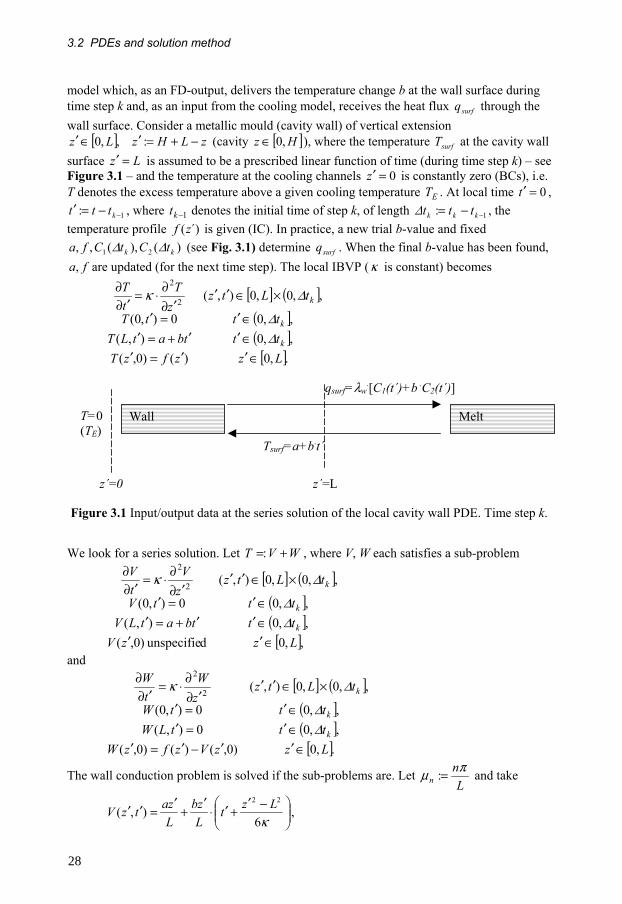
3.2 PDEs and solution method

Wall Melt T=0 (TE)

z´=0 z´=L

Tsurf=a+b.t´

qsurf=λw.[C1(t´)+b

.C2(t´)]

Figure 3.1 Input/output data at the series solution of the local cavity wall PDE. Time step k.

model which, as an FD-output, delivers the temperature change b at the wall surface during time step k and, as an input from the cooling model, receives the heat flux surfq through the wall surface. Consider a metallic mould (cavity wall) of vertical extension

[ ] zLHzLz −+=′∈′ :,,0 (cavity [ ]Hz ,0∈ ), where the temperature surfT at the cavity wall surface Lz =′ is assumed to be a prescribed linear function of time (during time step k) – see Figure 3.1 – and the temperature at the cooling channels 0=′z is constantly zero (BCs), i.e. T denotes the excess temperature above a given cooling temperature ET . At local time 0=′t ,

1: −−=′ kttt , where 1−kt denotes the initial time of step k, of length 1: −−= kkk ttt∆ , the temperature profile ´)(zf is given (IC). In practice, a new trial b-value and fixed

)(),(,, 21 kk tCtCfa ∆∆ (see Fig. 3.1) determine surfq . When the final b-value has been found, fa, are updated (for the next time step). The local IBVP (κ is constant) becomes

[ ] ( ]( ]( ]

[ ].,0)()0,(,,0),(,,00),0(

,,0,0),(2

2

LzzfzTtttbatLTtttT

tLtzzT

tT

k

k

k

∈′′=′∈′′+=′∈′=′

×∈′′′∂

∂⋅=′∂

∂

∆∆

∆κ

We look for a series solution. Let WVT +=: , where V, W each satisfies a sub-problem

[ ] ( ]( ]( ]

[ ],,0dunspecifie )0,(,,0),(,,00),0(

,,0,0),(2

2

LzzVtttbatLVtttV

tLtzzV

tV

k

k

k

∈′′∈′′+=′∈′=′

×∈′′′∂

∂⋅=′∂

∂

∆∆

∆κ

and

[ ] ( ]( ]( ]

[ ].,0)0,()()0,(,,00),(,,00),0(

,,0,0),(2

2

LzzVzfzWtttLWtttW

tLtzzW

tW

k

k

k

∈′′−′=′∈′=′∈′=′

×∈′′′∂

∂⋅=′∂

∂

∆∆

∆κ

The wall conduction problem is solved if the sub-problems are. Let L

nn

πµ =: and take

−′+′⋅

′+

′=′′

κ6),(

22 LztLzb

LzatzV ,

28

3.2 PDEs and solution method

( ) [ ] zdzzUzfL

WtzWtzW n

L

nn

nnn ′′⋅′−′⋅=′−′⋅=′′ ∫∑∞

=

)sin()0,()(2:,exp)sin(),(01

2 µκµµ .

Let )(Lfa = (constant) and define Lzazfzg′

−′=′ )(:)( .

If )(zg ′ has a Fourier sine series expansion ∑∞

=

′⋅=′1

)sin()(n

nn zgzg µ , then

bL

gWn

n

nn ⋅−−= 3

)1(2κµ

.

The initial temperature profile of the next time period, ),(:)(~ktzTzf ∆′=′ , is fixed by b and

)(~)()(~ zgLztbazf k ′+′

⋅⋅+=′ ∆ ,

( ))exp(1)1(2)exp(:~ 23

2kn

n

n

knnn tL

btgg ∆κµκµ

∆κµ −−⋅−⋅+−⋅= .

At the wall surface,

( )

( ) ( ).)()(:

exp123

exp)1(

exp)1(3

21

1

22

1

2

1

2

btCtC

tL

LLtbtg

La

tWbLL

tbazT

nn

nnn

nnn

nn

nnn

Lz

⋅′+′=

′−⋅−+

′⋅+′−−⋅+=

′−−⋅++′+=

′∂∂

∑∑

∑∞

=

∞

=

∞

==′

κµµκκ

κµµ

κµµκ

Here we are only interested in ktt ∆=′ . Thus )(),( 21 kk tCtC ∆∆ are locally fixed in time step k and, as a response to a new b-value from the melt model, the updating computational work of

Lzwsurf z

Tq=′

′∂∂⋅= λ becomes a linear operation only.

The )(1 tC ′ -series converges absolutely for every 0>′t , irrespectively of )(zg ′ , and the )(2 tC ′ -series converges absolutely for every 0≥′t . At the front, as T measures the

temperature above ET , then 0>>−≈ EI TTa , and 0)( ≡′zf . Here aL

gn

n

n ⋅−=µ

)1(2 , and the

)(1 tC ′ -series diverges at 0=′t , due to infinite initial heat flux. In this case, 212 Ct

aC

=′⋅

holds in general. This means that 022 =

+

′⋅=

′∂∂

=′

btaC

zT

Lz

is obtained at a time ctt ′=′

fulfilling atb c 21−=′⋅ , i.e. when the initial temperature difference between melt and wall is

halved. If necessary, because of the basic linear approximation of flux and temperature, the front time step should be subdivided into sub-steps much shorter than ct ′ . In practice the sub-step control at the front is activated, if the initial temperature difference melt-wall is reduced by more than a prescribed percentage during kt∆ . Behind the front, since )(Lfa = , i.e.

0)( =Lg , the )(1 tC ′ -series is expected to converge rapidly also at 0=′t . To cope with the singularity for 0=′t at the front, i.e. when the hot melt meets the cold metal, an improved initial time-substep is described in App. 2, where we replace the slowly converging series solution by an analytical square-root solution, according to Sec. 3.1.3.

29

Active-flow computation Flowchart 3.2

Estimation of viscosity parameters

0,, KTB B

Picture production

Passive-flow computation Flowchart 3.3

Results γ&,,,,, zr vvpTh at the end of filling,

and their time evolutions at a selection of nodes (bInj=True:) Times of injection Iteration statistics

Material data Pc,λ Linear phase-specific functions of T

ρ Phase-specific melt density

MT (all materials:) No-flow temperature

ML (semi-crystalline material:) Latent heat of solidif.β,0K Viscosity normed & pressure-related param.s

BTB, Viscosity temperature-related parameters n Power-law index

wλ Thermal conductivity of metal mould

wPc )(ρ Density times heat capacity of metal mould

Simulation parameters J Highest axial z-node level K Number of time steps N Highest series term wall solution NVr Highest series term velocity & viscosity z-factorzBeth Vertical transformation factor uPhi Number of node rays uFountL Number of fountain flow z-levels bInj Indicator for computing times of injection bInterp Indicator for using interpolation in h-iter. bFount Indicator for applying fountain flow bPhiEff Indicator for using effective flow angle dPhiEff Effective flow angle (per sector & side) FhEps Residual error bound in h-eqn 0=Fh FTEps Residual error bound per T-eqn 0=FT hEps_1 Upper bound h-distance between positions of negative and positive Fh puFT Armijo reduction limit in T-eqns 0=FT udT (active-flow:) Upper bound T-change per T-iter.uTIter Maximum number of NR (& backup) T-iter.s uTStepIter Maximum number of ArmijoT-step-iter.spTCrit Lower bound of T-reduction per time step

Flowchart 3.1 Data processing.

Cavity and wall geometry R (disk-shaped cavity:) Radius x,y (or star-shaped cavity:) Corners H Nominal height (half-gap width) of cavity

wH (constant:) Depth of cooling circuit in metal mould )}(,{ rHr w (or variable:)File with radial profile of ditto

Process parameters EI TT , Inlet and cooling temperatures

fillqV (volume controlled transfer to pressure ctrl:) % Cavity volume

filltV (or time-controlled ditto:) Time )}(,{ tQt Pairs of time and inflow rate values

RI PuP , Upper pressure bound & constant front pressure

30

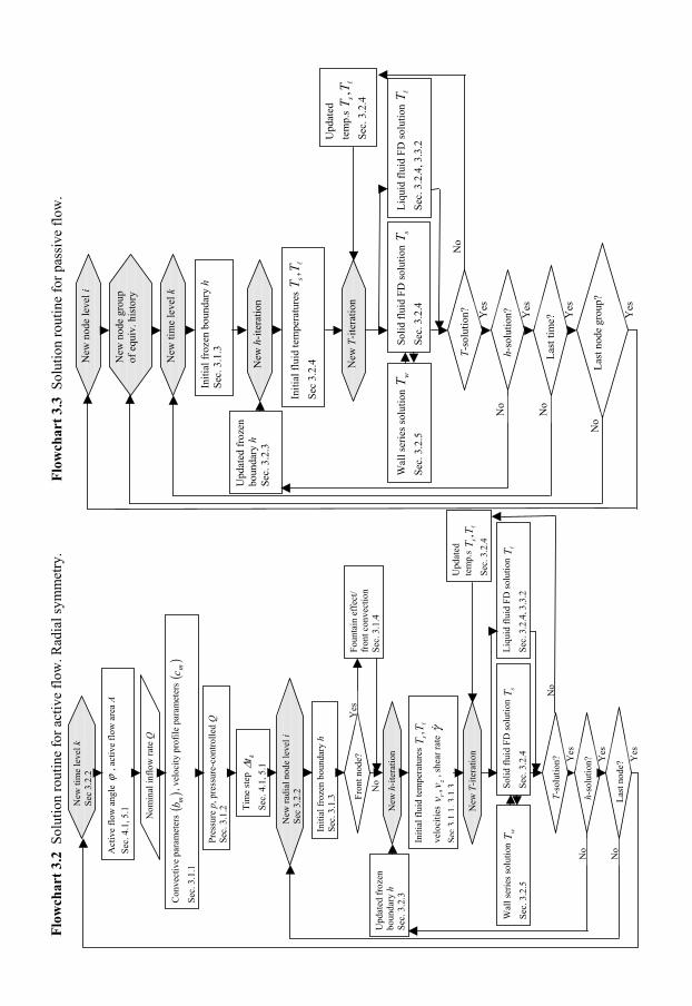
New

nod

e le

vel i

New

tim

e le

vel k

Initi

al fr

ozen

bou

ndar

y h

Sec.

3.1

.3

Initi

al fl

uid

tem

pera

ture

s lT

T s,

Sec

3.2.

4

Liqu

id fl

uid

FD so

lutio

n lT

Se

c. 3

.2.4

, 3.3

.2

Solid

flui

d FD

solu

tion

sTSe

c. 3

.2.4

W

all s

erie

s sol

utio

n wT

Se

c. 3

.2.5

Upd

ated

froz

en

boun

dary

h

Sec.

3.2

.3

h-so

lutio

n?

New

h-it

erat

ion

Last

tim

e?

No

Yes

Yes

N

o

Upd

ated

te

mp.

s lT

T s,Se

c. 3

.2.4

N

ew T

-iter

atio

n

T-so

lutio

n?

No

Yes

Flow

char

t 3.3

Sol

utio

n ro

utin

e fo

r pas

sive

flow

.

New

nod

e gr

oup

of e

quiv

. his

tory

Last

nod

e gr

oup?

Yes

No

No

Flow

char

t 3.2

Sol

utio

n ro

utin

e fo

r act

ive

flow

. Rad

ial s

ymm

etry

.

Act

ive

flow

ang

le ϕ

, act

ive

flow

are

a A

Sec.

4.1

, 5.1

Con

vect

ive

para

met

ers

()

mb, v

eloc

ity p

rofil

e pa

ram

eter

s (

)mc

Sec.

3.1

.1

Pres

sure

p, p

ress

ure-

cont

rolle

d Q

Se

c. 3

.1.2

Tim

e st

ep

kt∆

Sec.

4.1

, 5.1

Nom

inal

inflo

w ra

te Q

New

tim

e le

vel k

Se

c 3.

2.2

New

radi

al n

ode

leve

l i

Sec

3.2.

2

Initi

al fr

ozen

bou

ndar

y h

Sec.

3.1

.3 Fron

t nod

e?

Foun

tain

eff

ect/

fron

t con

vect

ion

Sec.

3.1

.4

Initi

al fl

uid

tem

pera

ture

s lT

T s,

velo

citie

s z

rv

v,

, she

ar ra

te γ&

Se

c3.

1.1,

3.1.

3

Liqu

id fl

uid

FD so

lutio

n lT

Sec.

3.2

.4, 3

.3.2

Solid

flui

d FD

solu

tion

sT

Sec.

3.2

.4

Wal

l ser

ies s

olut

ion

wT

Sec.

3.2

.5

Upd

ated

froz

en

boun

dary

h

Sec.

3.2

.3

h-so

lutio

n?

New

h-it

erat

ion

Last

nod

e?

No

Yes

Yes

Yes

N

o

Upd

ated

te

mp.

s lT

T s,

Sec.

3.2

.4

New

T-it

erat

ion

T-so

lutio

n?

No

Yes

3.3 FD scheme

3.3 FD scheme In this Section the FD-scheme is derived and examined. The discretization of the PDE (3.11) is made by control volumes in Sec 3.3.1, in such a way that truncation errors become small. Several potential FD schemes have been investigated in this project, but this thesis describes a time-implicit scheme only. Since the temperature is expected to fall rapidly near the cavity wall, the density of the gap-wise (axial), discrete node levels should increase towards the wall, and the transformation we find does not reduce the order of accuracy. Another principle is to base our discretization upon a conservative form of the PDE, in consideration of phase-specific, linear heat capacity and conductivity functions of temperature, according to our conclusions in Sec. 2.2.5. In Sec. 3.3.2 we investigate the existence and uniqueness of the solution of the discretized problem, and formulate operational conditions for the NR routine to converge. An FD-equation is said to be convergent if its solution approaches the PDE solution as the step sizes tend to 0. For linear and linearized well-posed PDEs in simple geometries, convergence in 2L -norm of one-step FD-schemes is guaranteed by consistency and stability, according to the Lax-Richtmyer equivalence theorem (e.g., [Strikwerda], p.222). Consistency, i.e. that the truncation error tends to 0 as the step sizes do, is guaranteed by our choice of FD scheme – see Sec. 3.3.1 – and by the convergence of our FD solution method – see Sec. 3.3.2. Stability means that the FD routine does not amplify errors. Although stability of a linearized scheme is no guarantee for overall stability, we investigate such schemes in Appendix 5, in order to identify crucial quantities for the nonlinear problem. As for fluid acceleration, the restrictions are similar to the well-posedness conditions in App. 4. But the possibility of instabilities due to 0↓h now becomes evident.

3.3.1 Control volume approach and truncation error Assuming one inlet at 0=r , we consider a node O at radius r and a surrounding small cavity volume with radial extension ),( 2

121 rrrr ∆∆ +− , axial extension z∆ and covering the whole

active flow angle actϕ , i.e. having the volume measure zrractV ∆∆ϕµ =: . The difference between the PDE-terms and the approximating FD-equation terms for one and the same temperature distribution is the truncation error. Consistency now means that the truncation error tends to zero if the step sizes ∆r , z∆ do. To prepare for an analysis by control volumes, we introduce a local coordinate system )~,~( zr surrounding node O. The third, angular, dimension is implicit. Also time is implicit in the non-dynamic PDE terms below, since all function evaluations are assumed to take place at the current time, i.e. without time error. The explicit equation at O represents the heat balance within a rectangle (control volume) n-w-s-e, the boundaries being placed half ways between O and each of its four neighbour nodes N, W, S and E. The eastward (flow direction) step size ∆r is assumed fixed; thus e w r= − =: /∆ 2 and ∆r e w= − . However, the northward (vertical) step size z∆ is allowed to vary; thus n s≠ − >( )0 may hold in |)|(: snsnz +=−=∆ . This makes the control volume approach useful, also in representing the energy weight of the corresponding FD-equation, by the volume measure Vµ . The local coordinates )~,~( zr of the surrounding node points become N n: ( , )= 0 2 , W r: ( , )= −∆ 0 , S s: ( , )= 0 2 , E r: ( , )= ∆ 0 – see Figure 3.2.

32

3.3 FD scheme

Figure 3.2 Control volume.

local radial position r~

r∆2/r∆2/r∆−r∆− 0

local axial position z~

||2 js−

|| js−

jn2

jn

OW

S

N

E

n

w

s

e 0

level j+1

level j

level j-1

level i-1 level i level i+1

jz∆

r∆

First, consider the conduction term of the PDE, represented by

rdrrzdzT

zrdzddrr

zT

zI

e

w

n

sact

e

w

n

sPDEcond

act~)~(~~~)~(:

0, +

⋅=+

= ∫ ∫∫ ∫ ∫ ∂

∂λ∂∂ϕϕ

∂∂λ

∂∂ϕ

.

A PDE is said to be in conservative form (see, e.g., [Özisik], p.5), if the coefficients of the derivative terms are constant. Here the conductivity λ (cf. Sec. 2.2.2) is assumed to be a linear function of temperature, T10: λλλ += . Letting TTTL ⋅+= )(:)( 12

10 λλ the integral

takes the conservative form

rdrrzL

zLrdrrzd

zTLI

e

w snact

e

w

n

sactPDEcond

~)~(~)~(~)(2

2

, +

−

⋅=+⋅= ∫∫ ∫ ∂

∂∂∂ϕ

∂∂ϕ .

In a more general setting, introducing zLrrzru act ∂

∂⋅+⋅= )~(:)~,~( ϕ , the integral is of type

[ ] rdsrunruIe

wPDEcond

~),~(),~(, ∫ −= .

Assume that u is an analytic function of )~,~( zr in a neighbourhood of (0,0), i.e. of node O.

Then u can be described locally by the power series ∑∞

=

=0,

~~:)~,~(ji

jiij zruzru , convergent for

sufficiently small |~||,~| zr . Now the integral can be evaluated by termwise integration and use of 2/rwe ∆=−= as

( )( ) [ ]

K++++−+=

=−−+

=−−+

= ∑∑∑∞

=

∞

=

+∞

=

++

zrusnrusnruzru

snmrusnwe

iuI

m j

jjm

m

jmji

jjiiijPDEcond

∆∆∆∆∆∆

∆

32112

13303

220201

0 12

12

,20,

11,

)||()||(

|)|(2)12(1

1

where higher order terms of ∆r , ∆z are omitted. If T is analytic at O, then termwise u, T power series identification in

33

3.3 FD scheme

∂∂+

∂∂⋅+⋅=

∂∂⋅+⋅=

zTT

zTrr

zLrrzru actact 00)~()~()~,~( λλϕϕ

yields

∑∑

∑∑−

=

+

=−+−−+−

=

+

=−+−+

⋅⋅++⋅⋅+

⋅⋅++⋅⋅=

1

0´

1

1´´´´1,1´11,10

0´

1

1´´´´1´,11,0

´)1(

´)1(

i

i

j

jjijjiijiact

i

i

j

jjijjiijiactij

TTjTj

TTjTjru

λλϕ

λλϕ

In order to cancel the leading term of Icond PDE, by a matching FD-discretization FDcondI , we evaluate and weigh λ , T at N, O, S. The basic approximation is

( )[ ] .)(

~)~(

,0~,0~

2221

,0~,0~

,

zzL

zLwewer

zL

zL

rdrrzL

zLI

V

srnrsrnract

e

w snactPDEcond

∆µ

∂∂

∂∂

∂∂

∂∂ϕ

∂∂

∂∂ϕ

⋅

−

=−+−⋅

−

⋅≈

≈+

−

⋅=

====

∫

Consistent heat flow across the borders between adjacent control volumes is accomplished by using the implicit central difference scheme

zs

TTT

nTT

Tzs

TLTLnTLTL

I VSOs

ONn

VSOONFDcond ∆

µλλ∆µ

⋅

−−

−=⋅

−−

−=

||2)ˆ(

2)ˆ(

||2)()(

2)()(

:, ,

where )(:ˆ21

ONn TTT += , )(:ˆ21

SOs TTT += .Then .)||()||( 3

2112133

0322

0231

,, K+++−−−=− zrusnrusnruII FDcondPDEcond ∆∆∆∆

If 0|)|( ≠→− constzsn p∆ as 0→z∆ , i.e. n s O z p− =| | ( )∆ , the error magnitude becomes )( ]2,min[2 p

V zrO ∆+∆⋅µ . Hence it is unaffected for 2≥p (where fixed step size corresponds to ∞→p ). Since the steepest temperature variation occurs at the mould wall and since freezing is in focus, the axial step sizes z∆ should decrease towards the wall. Although p = 1 serves these demands, including, e.g., any geometric series of diminishing node distances, the disadvantage is a reduced order of accuracy. Instead, we use a transformation from ],0[ Hz∈ to a uniform grid in the computational domain ζ ∈[ , ]0 1 , generated by (cf. [Özisik], p.315):

;11:,:)(,

ln)(ln

−+=

−

+==

ββ

β

βζ B

HzHz

zABzA

where β is a parameter, β > 1. The inverse transformation is

z BB

H= ⋅ −+

⋅β ζ

ζ( )1

1.

Here a constant space step ∆ζ is applied to the computational domain. A full transformation means that also the PDE is transformed. However, we prefer to work in z-space – alas a non-constant step size z∆ . The leading transformation derivatives are

34

3.3 FD scheme

.

8ln)1()1(

ln

2)(

),0(4ln

)1(

ln

1)(

232

22

2223

2

2

22

ζ

ζζ

ζ

ζ

ββ

ζ

ββ

ζ

BBHBB

HzBH

zz

BBHB

HzBH

z

⋅⋅⋅−+=

−⋅⋅

=′′

>⋅⋅⋅

+=

−⋅⋅

=′

As for the decisive (dimensioning) p-value we realize that, since 0)( >′′ zζ for 0>z ( 0>ζ ), )(zζ ′ will increase by z. Hence the critical behaviour is close to the wall surface, where Hz = , so 1≈ζ , and consecutive step sizes satisfy

)(8

)1(|| 222

zOzBHBsn ∆=∆⋅−→− .

Thus 2≥p everywhere (when 0↓ζ∆ ), and the truncation error is unaffected.

As for the conservative form of the two convection terms, the coefficient lρ (cf. Sec. 2.2.2) is assumed constant but l,Pc (cf. Sec. 2.2.1) is a linear function of T, TcccP 10, : +=l . Consider the internal energy ( ) TTccTU ⋅+= 12

10:)( lρ and let v denote the velocity vector. By the

equation of continuity (the fluid is incompressible) the convection terms can be put into the conservative form

[ ])(div)(graddiv)(

)grad()()( ,,

TUTUTU

TTczTv

rTvTc PzrP

vvv

v

=+⋅=

=⋅=

∂∂+

∂∂⋅

•

•llll ρρ.

By use of Gauss’s theorem the corresponding PDE-integral on the control volume can be written

[ ] [ ]{ } [ ] [ ]{ } rdrrUvUvzdUvrrUvrrIe

wsznzact

n

swreractPDEconv

~)~(~)~()~(, +−⋅++−+⋅= ∫∫ ϕϕ .

By letting Uvrrzru ract ⋅+⋅= )~(:)~,~( ϕ , bounded for )~/(1 rrvr +∝ if 0~ →+ rr , the first integral of PDEconvI , becomes

{ } zdzwuzeuIn

sPDEconv

~)~,()~,(:,1 ∫ −= .

In a standard up-winding FD-scheme PDEconvI ,1 is approximated (cf. Fig. 3.2) by zuuI WOFDconv ∆−= )(:,1 .

Assuming a series expansion ∑∞

=

=0,

~~:)~,~(ji

jiij zruzru , the error becomes

( )

).()||(

1|)|(

2]2,min[22

11213

30432

20

10

0,

11

2

12

,12,1,1

pV

i

ii

jm

jj

m

m

jmFDconvPDEconv

zrOsnruzruzru

zruj

snruII

∆∆µ∆∆∆∆∆

∆∆∆

+⋅=+−+−=

=−++−−⋅=− ∑∑

∞

=

∞

=

+++

+

K

If we let Uvrrzru zact ⋅+⋅= )~(:)~,~( ϕ , the second integral of PDEconvI , turns into

35

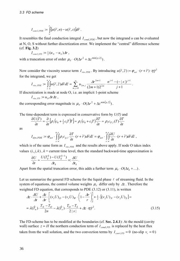
3.3 FD scheme

{ } rdsrunruIe

wPDEconv

~),~(),~(:,2 ∫ −= .

It resembles the final conduction integral PDEcondI , , but now the integrand u can be evaluated at N, O, S without further discretization error. We implement the “central” difference scheme (cf. Fig. 3.2) ruuI SNFDconv ∆)(: 2

1,2 −= ,

with a truncation error of order )( ]2,min[2 pV zrO ∆+∆⋅µ .

Now consider the viscosity source term PDEviscI , . By introducing 2)~(:)~,~( γηϕ &⋅+⋅= rrzru act for the integrand, we get

∑∫ ∫∞

=

+++

+−−⋅

+==

0,

11

2

12

,2, 1|)|(

2)12(~~)~,~(:

jm

jj

m

m

jm

n

s

e

wPDEvisc j

snmruzdrdzruI ∆ .

If discretization is made at node O, i.e. an implicit 1-point scheme zruI OFDvisc ∆∆=:, ,

the corresponding error magnitude is [ ])( 2,min2 pV zrO ∆+∆⋅µ .

The time-dependent term is expressed in conservative form by U(T) and

( )[ ] ( )tTTc

tTTccTTcc

ttTU

P ∂∂=

∂∂+=+

∂∂=

∂∂ )()(

,10121

0 llll ρρρ

as

zdrdrrtUzdrdrr

tTcI

n

s

e

wact

n

s

e

wpactPDEdyn

~~)~(~~)~(: ,, ∫ ∫∫ ∫ +⋅∂

∂⋅=+⋅∂∂⋅= ϕρϕ ll ,

which is of the same form as PDEviscI , and the results above apply. If node O takes index values ),,( kji , k = current time level, then the standard backward-time approximation is

kk

kij

kij

tU

tTUTU

tU

∆∆

∆:

)()( 1

=−

≈∂

∂ −

.

Apart from the spatial truncation error, this adds a further term )( K+∆⋅ kV tOµ .

Let us summarize the general FD scheme for the liquid phase l of streaming fluid. In the system of equations, the control volume weights Vµ differ only by z∆ . Therefore the weighted FD equation, that corresponds to PDE (3.12) or (3.11), is written

[ ]

)15.3( .||2

)ˆ(2

)ˆ(

)()(1)()(

2

21

γη∆λλ

∆∆∆

∆∆∆

&⋅+−

⋅−−

⋅=

=−⋅+

−⋅−⋅+⋅

zsTT

TnTT

T

UvUvrrUvUv

rz

tUz

SOs

ONn

SzNzWrOr

The FD-scheme has to be modified at the boundaries (cf. Sec. 2.4.1): At the mould (cavity wall) surface Hz = the northern conduction term of FDcondI , is replaced by the heat flux taken from the wall solution, and the two convection terms by 0,1 =FDconvI (no-slip 0=rv )

36

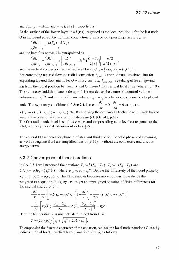
3.3 FD scheme

and ||2)(,2 suuzrI SOFDconv −⋅= ∆∆ , respectively. At the surface of the frozen layer ),( thz r= , regarded as the local position n for the last node O in the liquid phase, the northern conduction term is based upon temperature MT as

n

TLTLzL OM

n

)()(

2/

−≈

∂∂

and the heat flux across h is extrapolated as

||2/

2/||2

)ˆ(2/2/ sn

nsTT

TzL

zL

zL SO

snnn +

⋅

−−

∂∂+

∂∂≈

∂∂ λ ,

and the vertical convection term is replaced by [ ]SzOznz UvUvUv )()()( 21 −⋅− .

For converging tapered flow the radial convection 1convI is approximated as above, but for expanding tapered flow and nodes O with z close to h, FDconvI ,1 is exchanged for an upwind-ing from the radial position between W and O where h hits vertical level z (i.e. where 0=rv ). The symmetry (middle) plane node 00 =z is regarded as the centre of a control volume between 2/1zn = and nzs −== − 2/1 , where 11 zz −=− is a fictitious, symmetrically placed

node. The symmetry conditions (cf. Sec 2.4.1) mean 0=∂∂zT , 0=

∂∂zvz at 0z , and

)()( 11 −= zTzT , )()( 11 −−= zvzv zz etc. By applying the ordinary FD-scheme at 0z , with halved weight, the order of accuracy will not decrease (cf. [Özisik], p.47). The first radial node level has radius rr ∆= and the preceding node level corresponds to the inlet, with a cylindrical extension of radius r∆2

1 .

The general FD schemes for phase l of stagnant fluid and for the solid phase s of streaming as well as stagnant fluid are simplifications of (3.15) – without the convective and viscous energy terms.

3.3.2 Convergence of inner iterations In Sec 3.3.1 we introduced the notations )(:ˆ

21

ONn TTT += , )(:ˆ21

SOs TTT += and ( ) TTccTU ⋅+= 12

10:)( lρ , where TcccP 10, : +=l . Denote the diffusivity of the liquid phase by

)()(:)( , TcTT P llll ρλκ = . The FD-character becomes more obvious if we divide the weighted FD equation (3.15) by z∆ , to get an unweighted equation of finite differences for the internal energy )(TU :

[ ]

.||2

)ˆ(2

)ˆ(1

)()(2

11)()(1

2γηκκ∆

∆∆

∆∆∆

&ll =

−⋅−−⋅⋅−

−⋅+

−⋅−⋅+

sUUT

nUUT

z

UvUvzr

rUvUvrt

U

SOs

ONn

SzNzWrOr

Here the temperature T is uniquely determined from U as

++= ll ρρ /2)/2( 1

200 UcccUT .

To emphasize the discrete character of the equation, replace the local node notations O etc. by indices – radial level i, vertical level j and time level k, as follows

37

3.3 FD scheme

),,(:),(: kjikij

kij

kij tzrTTTUU == .

During an h-iteration, a trial value of the frozen layer surface ),( ki trhh = is fixed. Then

zr vv , and γ& become locally fixed, but η and (maybe) lκ depend upon T. The upper index k is used to mark this implicity for η , lκ , making the (unweighted) FD equation nonlinear:

( )

( ) )16.3(.||22

1

21

21,2/1,,

1,2/1,,

1,1,,1,1,,,1,1,,1

ijkij

j

kji

kijk

jij

kij

kjik

jij

j

kjijiz

kjijiz

kjiijir

kijijr

k

kij

kij

sUU

nUU

z

zUvUv

rUrrvUv

tUU

γηκκ∆

∆∆∆

∆

&ll ⋅=

−⋅−

−⋅⋅−

−+

−−+

−

−−

++

−−++−−−

In the inner iterative procedure for the active-flow cavity region a system of 1+J equations of type (3.16) is solved for ( )J

jkijU 0=

(in reality for ( )Jj

kijT 0=

), subdivided into two disjoint sets,

of liquid and solid fluid, modified at the boundaries and simplified in the solid phase. In each phase of state let the system be written 0f = (LHS – RHS of (3.16)). An iteration of the Newton-Raphson (NR) method means that the vector T of T-variables is changed by an amount u satisfying fGu −= , where f and the tri-diagonal Jacobian matrix G are evaluated at the current T-iterate. Here Thomas’s algorithm, i.e. simple LU-factorization (e.g., [Özisik], p.50) is well suited, producing the solution u by O(J) operations. For the solid phase and for the whole passive-flow region of the cavity, the viscous energy term disappears. Then if κ does not depend upon temperature, G becomes constant, i.e. (3.16) is just a set of linear equations (and only one NR-iteration is needed).

For the general iterative procedure to be well-defined, G needs to be non-singular. We will show that G is strictly diagonally dominant. Let the liquid phase correspond to the vertical levels ],0[ jhj∈ , with weights || jjj snz +=∆ , || jj sn ≤ .

Moreover, let

+⋅= ijz

j

kij

jN vnT

a ,21

,

)(: lκ

,

−⋅= ijz

j

kij

jS vsT

a ,21

, ||)(

: lκ. We focus on the general

expression, i.e. jhj <<0 . The three non-zero elements in G-row j are

1,1,,1,

,,2,

2,

,

1,1,,1,

)()()(

1)(

)(

+++

−−−

⋅−=

++

−⋅++⋅=

⋅−=

jSkjiPjj

jSjNB

kij

kijP

ijkijijr

kj

kijPjj

jNkjiPjj

aTcG

aaTTB

Tcrv

tzTcG

aTcG

ll

ll

ll

ll

&

ρρ

γη∆∆

∆ρ

ρ

Assume that conduction dominates over vertical convection, in the sense that 0, >SN aa . This is a numerical and not a physical restriction, since it can be accomplished by sufficiently small step lengths ( ) jh

jjz 0=∆ in any temperature region of interest. Now all the terms of jjG are

positive, since 0, >ijrv (upwinding) and 0>B (Arrhenius factor for real materials, cf. (2.4)). The non-zero elements in column j fulfil

0)()(

1)(|||||| 2,

2,

,,1,1 >

−⋅++⋅=−− +−

Bkij

kijP

ijkijijr

kj

kijPjjjjjj TT

BTcr

vt

zTcGGGll

ll

&

ργη

∆∆∆ρ .

Therefore G is an M-matrix ([Ortega], p.223), strictly (and irreducibly) diagonally dominant.

38

3.3 FD scheme

Hence (e.g., [Ortega & Rheinboldt], p.48) G is invertible with 0G >−1 , and the NR-iterates are well-defined. Since the diagonal G-elements are positive, the diagonal dominance also ensures that the eigenvalues have a positive real part. The temperature vector ( ) jh

jkijT 0

:=

=T varies in an

open, convex set 1+⊂ jhT RD , },{: 1 jTTTRD k

ijBjh

T ∀<<+∈= ∞+ εT , where BT is defined in

(2.4), and )0(>ε , ∞T are artificial bounds. Now ([ibid.], p.143) fT → is a one-to-one mapping in TD , and 0f = has at most one solution in TD . We want to show that a solution always exists, or else that unacceptably high or low temperatures (above ∞T or below ε+BT ) can be identified. Through a variable transformation – the mapping VT → , jV

Bkij eTT +=: , i.e.

( )Bkijj TTV −= ln: – the new variable vector ( ) jh

jjV 0:

==V defines a new mapping fV ~→ ,

))((:)(~ VTfVf = in the open, convex set },{: 1 jVVVRD jBjh

V ∀<<∈= ∞+V , where

εln:=BV , )ln(: BTTV −= ∞∞ . In theory, 0=ε and +∞=∞T , i.e. −∞=:BV and +∞=∞ :V , are possible. In case )(Tlκ and/or )(, TcP l are strictly decreasing functions of T, the positivity constraints 0, >SN aa will imply a theoretical bound +∞<∞T . In practice, the acceptable temperatures of the filling phase are far below the zeroes of )(Tlκ , )(, TcP l and any application that leads to a solution above these practical acceptance limits should be interpreted as non-solvable. The Jacobian )(~ VG of )(~ Vf satisfies ( ) )()()(~ jVeDiagVTGVG = , i.e. with

k

jPBP t

zTcTc

∆∆

ερβ ⋅+⋅= ∞ )](),(min[: ,, lll the non-zero elements in column j fulfil

( )

jijkijj

Vij

kijj

V

jjjjjjV

jjjjjj

BzBeze

GGGeGGG

jj

j

αγη∆βγη∆β :2

|||||||~||~||~|22

,1,1,1,1

=≥+>

>−−⋅=−−−

+−+−

&&

This lower bound )0(>jα is well-defined whenever ∞<< Vij

kijj eBz βγη∆ε /2& . Thus )(~ Vf is

uniformly monotone in VD . For −∞=:BV , +∞=∞ :V ( [ibid.], p.143) f~ is a homeo-morphism

of 1+jhR onto 1+jhR , and 0Vf =)(~ , i.e. 0VTf =))(( , has exactly one solution T.

In order to apply the Newton-Mysovskii Theorem ([ibid.], p.412) we have to show that (i): G satisfies a Lipschitz condition, and (ii): 1−G is bounded above, for some norm.

Property (i) follows at once, since we realize that f is twice-continuously differentiable.

To verify (ii) we start by showing that G is bounded below. Take jjhjα

εα

],0[min1:∈

⋅= and let

min)(Gλ denote the smallest absolute eigenvalue of G. Now since all diagonal elements { }jjG

are real and positive, the Gersgorin Circle Theorem ([ibid.], p.49) yields αλ ≥min)(G in TD .

The 2L -norm of the real matrix G is )(sup: max21

22

GGGxGx

Tλ===

. This is the largest

singular value of G, satisfying ([Horn & Johnson], p.176) maxmax |)(|)( GGG λλ ≥T . Hence we get a positive lower norm bound in TD , αλλ ≥≥≥ minmax2 |)(||)(| GGG .

39

3.3 FD scheme

Next we will use this lower bound to derive a general upper bound for 2

1−G .

The 2L -norm of 1−G is ( ) ( )GGGG TTmin

1max2

1 1)( λλ == −−G .

The products of all eigenvalues and all singular values, respectively, satisfy ([ibid.], p.171)

( ) ∏∏==

==jh

jj

jh

j

Tj

00)()(det GGGG λλ .

Hence

( ) ( ) 1

00minmaxmin2 )()()()()( +

==≥=≥⋅=⋅ ∏∏ jh

jh

jj

jh

j

Tj

Tjh

TTjh αλλλλλ GGGGGGGGGG

and finally ( ) MjhjhT :)(1 1

2min21 =≤= +− αλ GGGG , (3.17)

a general upper norm bound. This shows property (ii). (In particular, if we assume that G is normal, i.e. (e.g., [Meyer], p.547) has a complete set of jh+1 orthonormal eigenvectors { }jz , corresponding to the eigenvalues { }jλ , then any unit

length eigenvector z, corresponding to )(min GGTλ , can be written ∑=

=jh

jjjp

0zz with

∑=

∗ ==jh

jjp

0

2||1 zz , where ∗z denotes the transposed complex conjugate of z. We get

1

)()()(

22222

minmin

⋅=⋅≥=

=

===⋅=

∑∑∑∑∗

∗∗∗

ααλλλ

λλ

jj

jjj

jjjj

jjjj

TTT

pppp zz

GzGzGzGzzzGGGG

and receive the stronger bound M:12

1 =≤− αG in TD .)

Now if the first NR-iterate )0(T is chosen such that the start direction )()(: )0()0(

1)0( TfTGu −−=

has a sufficiently small norm, then the Newton-Mysovskii Theorem guarantees that the iterates converge to the unique solution. In practice, as a security measure (see Sec. 3.2.4) we evaluate the objective function ff TF =: , and use the damped Newton method if necessary. According to [Dennis & Schnabel], p.121, the problem properties imply that the damped NR iterations k lead to 0Tf =)( )(k for some 0≥k , or

0)(

lim2)(

)()( =∇

∞→k

kT

k

k

F

u

uT.

The directional derivative satisfies, using inequality (3.17),

M

FT2

221

22

21

22

2

222 f

fG

f

fG

fu

u≥≥=

∇−−

,

i.e. it tends to 0 only if 2

f does, and not because F∇ and u are orthogonal. Thus the inner iterative procedure converges globally to a solution of 0f = , irrespectively of starting point. In theory we have to accept that the bounds ε+BT , ∞T may be violated during the iteration process, before the solution is found.

40

4.1 Special modelling: Radial flow

4 Application: Circular plate Our method has been implemented for two different applications. The first type, disk shaped cavities, is studied in this Chapter. In Sec. 4.1 we are modelling the disk flow. The discrete time steps are chosen such that the radial expansion per step becomes constant. A time step is primarily determined from the (prescribed) inflow rate and the volume to fill, but we also consider the shrinkage effect that solidification has upon the volume to fill, due to a density variation by temperature. In a true circular case a front expansion rate according to the distance model is uncontroversial. In Sec. 4.2 two specific materials, one amorphous poly-carbonate (PC) and one semi-crystalline polyethylene (HDPE) are modelled. Data for the two materials come from the data base of the FEM-FD-program Moldflow (of Moldflow Corp.). We have made a somewhat critical comment on the Moldflow PVT, 2nd order viscosity and enthalpy models. Unlike the 3D-capacity of Moldflow in modelling mould cavity and metal mould, we rely on a 2D flow model and a 1D cooling model, describing the distance from the cavity wall surface to the cooling lines as radially varying only. In Sec. 4.3 the comparison runs, two of each material, are discussed. The Moldflow modelling and runs have been performed by [Valtonen]. First the time evolution of pressure is studied. We have tried both the isothermal viscosity model and the extension described in Sec 3.1.2. Next the tempera-tures are investigated, as to time evolution as well as radial distribution and vertical profile at the end of filling. Our two front models are compared, and as an alternative a constant depth of the cooling lines is tried. Finally the radial profiles of the frozen layer (no-flow temperature isotherm) at the end of filling are evaluated. In Sec. 4.4 we are investigating whether our built-in, more advanced material models have any visible effect upon the basic HDPE run. In this respect a latent heat of crystallisation and a phase-specific linear heat capacity, a phase-specific linear heat conductivity and a pressure dependent viscosity are evaluated. In Sec. 4.5 some aspects of the method performance are documented, primarily the number of outer (h) and inner (T) iterations, and their relation to the number of vertical node levels.

4.1 Special modelling: Radial flow Because of the expansion of the frozen layer, the radial flow has a vertical component compensating for the contraction due to solidification (as lρρ >s ). When radial level i of time level k is treated numerically, by the method of radial marching, the vertical expansion

kih '∆− (h denotes non-frozen height) of the frozen layer at the preceding radial levels

1,,1' −= ii K during kt∆ is known. If the phase-change factor (cf. Sec. 3.1.3) is denoted 1: −= lρρα s and kϕ is the average active flow angle during kt∆ (with πϕ 2=k in the

circular application), then the “lost” liquid volume up to i is

∑−

=− ⋅⋅−=

1

1'''1 2:

i

iik

ki

ki rrhq ∆ϕ∆α .

To estimate a nominal mean radial velocity, the melt at i is assumed to move radially from 2dri − to 2dri + , where the local distance d is given by the inflow rate kQ and

drhqtQ ikik

kikk

11 2 −

− ⋅=− ϕ∆ . The nominal velocity becomes

i

kik

kkik

k

kir rh

tqQtdv 1

1, 2

: −−

⋅−

==ϕ

∆∆

.

In our time-implicit implementation kirv , is based upon k

iki hq , instead of 1

1 , −−

ki

ki hq .

41

4.2 Materials data

Analogously, the front position is corrected (afterwards). During kt∆ the front is expected to expand from 2rrk ∆− to 2rrk ∆+ , by filling an area kA∆ . The “lost” liquid volume of the previous time level 1−k is considered when the new time step kt∆ is determined by the nominal half-width H and 1

12 −−+⋅= kkkkk qAHtQ ∆∆ .

After that, the rate is corrected to measure the filling of new area exclusively, k

kkkk tqQQ ∆1

1: −−−= .

4.2 Materials data Simulation runs for comparison have been performed by [Valtonen], using the commercial software Moldflow of Moldflow Corp., version 2.0.1. From the Moldflow (“Mfl” below) data base of standard materials, one amorphous thermoplastic – the polycarbonate Makrolon 2205 of Bayer AG (“PC“ below) – and one semi-crystalline material – the high density polyethylene Lupolen 5031 L of Basf AG (“HDPE” below) – were (arbitrarily) chosen. One run of normal processing conditions (“warm” below) and one of low temperature filling (“cold” below) were simulated for each material. The circular cavity radius was chosen extreme (40 cm) to provoke freezing. The plate thickness is 3 mm and the inlet is (unintentionally) 1.5 cm from the plate centre, i.e. the inlet to wall distance varies between 38.5 and 41.5 cm in the Mfl runs. The comments below on Mfl are solely based upon the four simulation runs. According to the materials documentation, the Mfl model assumes constant heat conductivity, constant specific heat and the existence of a no-flow temperature. The no-flow temperatures deviate a lot from the reported melting point C 131 o=MT for Lupolen (MatWeb, www.matweb.com) and from the glass transition temperature C 148 o=GT for Makrolon (Bayer product information, www.makrolon.com/eigenschaften), which is confusing – also see comment on Fig. 4.1 below. No specific modelling of the latent heat of crystallization seems to exist. All convective heat transfer in the z-direction is ignored ([Kennedy], p.71). The shear rate is approximated as zvr ∂∂≈γ& ([ibid.], p.70). The density variations are described by a thermodynamic PVT model – cf. [ibid.], p.28-29, or considered as incompressible ([ibid.], p.60). The underlying data points for pressure, specific volume and temperature, as well as the model coefficients, are documented in the Mfl data base. However, as can be seen from Figure 4.1 – which we have constructed from the 13 given calibration points of Lupolen and which shows the two phase-specific Mfl sub-models – the modelling routine seems imperfect: as we understand Mfl data, the sub-model for the liquid phase does not fit the calibration points (and the Mfl no-flow value C20 1 o is lower than can be estimated from Fig. 4.1). In order to imitate the Mfl model, we have to use almost the same density in both phases – and therefore the contraction effect of solidification becomes (unrealistically) small. (According to the Mfl data base, the generic densities V/1=ρ of the solid and liquid phases are 0.952 and 0.809, respectively; the latter value fits the data points in Fig. 4.1 but is contradictory to the sub-model for the liquid phase.) As to viscosity, the user may choose between a 1st and a 2nd order model – cf. [Kennedy], p.11. According to the 2nd order model, ηln is a 2nd order polynomial of T and γ&ln , and no theoretical, asymptotic results are used – cf. Sec. 2.2.3. Such modelling is a risky business, especially if the calibration points are few and close – see Figure 4.2, where the 6-parameter 2nd order Moldflow model and the 6 underlying data points of Makrolon are shown. There are two kinds of questionable behaviour: an increase by γ&ln for fixed T at low γ&ln -values, and an

42

4.2 Materials data

increase by T for fixed γ&ln , shown by curves crossing at high γ&ln -values. The latter model weakness is merely theoretical – the shear rate is below 410 1−s here – but the former is non-negligible: in our normal processing run for Makrolon, run PC-warm, 21% of the time-node registrations fall within the first questionable region. Therefore the 2nd order viscosity model has not been chosen here. The 1st order model is a power-law model with multiplicative temperature dependence, of type )exp( cT− , making the deviations from an Arrhenius-type model relatively small. For Makrolon the Mfl viscosity shows a 20-fold decrease from flownoT − to IT – a support for our non-isothermal model.

The materials data of the basic simulation runs are found in Table 4.1, where our fitted values to the Mfl density and viscosity models are marked by asterisks. Data seem somewhat uncertain, since e.g. Makrolon heat capacity CJ/kg 1170 o and thermal conductivity

C W/m0.2 o are found in the online materials database MatWeb.

In the Mfl runs, the metal mould is modelled by [Valtonen] as a square block with sides 100 cm and height 50 cm. Two circular cooling circuits of diameter 30 mm, with c/c distance 10 cm are modelled – cf. Figure 4.3. For each circuit the distance between the inlet and outlet channel legs is 40 cm and the cross leg is situated 30 cm from the closest mould side surface. Thus the horizontal distance between the points on the cavity wall surface and the centre of the closest cooling line varies between 0 and 20 cm, with an average of 8.9 cm, and the overall distance to the closest tube wall varies between 3.5 and 19.1 cm, with an average of 9.15 cm – see Figure 4.4, where the radial variation is shown (inlet at 0=r ). Four Mfl nodes, selected for special study, are also marked. Our FD program accepts a constant distance WH to the closest tube wall or a specified radial distribution, like the one in Fig. 4.4. The standard Mfl wall parameters are 3kg/m 7800=wρ , C W/m29 o=wλ and CJ/kg 460,

o=wpc .

43

4.2 Materials data

Table 4.1 Materials data used in basic FD runs

Lupolen 5031 L Makrolon 2205900* 1120*925* 1180*0.175 0.1733643 1700802.2* 0.06195*1139.0* 5552.0*-273.2 -273.20.4403 0.73510 ---120 170

sλλ =l

spp cc ,, =l

LHn

3kg/m3kg/m

lρ

BBT

nsPa ⋅01)/(

0 KeK nTTB B −− ⋅⋅= γη &

sρ

CoCo

CoJ/kg

flownoT −

CW/m o

CJ/kg o

44

4.3 Comparison runs

4.3 Comparison runs 4.3.1 Pressure distribution In the Moldflow (Mfl) runs, transfer to pressure controlled filling takes place when 98% of the mould cavity is filled. Before that, filling is controlled by the inflow rate. In our FD program this is implemented as a transfer to constant pressure at the inlet, as it (the pressure) is computed when 98% of the volume is filled, and kept for the rest of the filling. The time evolution of pressure, at four selected nodes, is shown in Figure 4.5. The vertical lines show the nodal front passages and the end of filling. Notice that the Mfl pressure registrations occur a little before the (in another data file) registered times of front passage. The steep increase of the Mfl pressure values immediately before the pressure-controlled filling (the horizontal pressure lines in Fig. 4.5) is probably due to the asymmetric placement of the inlet. The FD runs presume symmetry. Up to the end of filling the pressure deviations between FD and Mfl are relatively small for HDPE (in both runs). We have also tried isothermal pressure values (not shown) and as expected – cf., e.g., [Agassant et al.], pp.141,146 – these are much lower, even if based upon the average viscosity, and this simplifying model is therefore definitely rejected here. For PC the Mfl and FD pressure evolutions follow different increase rates (in both runs). Figure 4.7 below shows that the inflow rates are of the same magnitude in all runs. The Mfl pressure evolutions in Fig. 4.5 are almost identical for both materials, while in the FD runs the clear difference between the power law index n values – see Tab. 4.1 – has an impact upon pressure propagation, according to (3.6). But shear thinning is of course also temperature-dependent – see Fig. 4.7 for process temperatures IT and ET . Our logarithmic pressure model is clearly visible for 0=r in Fig. 4.5b, and its systematic deviation from the Mfl evolution may indicate a model error. But we are somewhat sceptical to the Mfl results for both runs PC-warm and PC-cold – see Fig. 4.10 below, where the differences between the top and bottom frozen layers, i.e. the vertical distances ×−× and ∇−∇ , are big.

45

4.3 Comparison runs

46

4.3 Comparison runs

4.3.2 Temperature distribution All four runs show similar patterns of node temperature evolution– see Figure 4.6 for the vertical average temperatures in run HDPE-warm. For Mfl there are two data files of information – on the selected nodes and on the corresponding finite elements (at the end of filling, only). For most nodes, the final FD temperatures lie between and/or close to these two values. Although there is no severely divergent Mfl-FD pair of evolution curves, the average deviation is more than 5 Co for all nodes in all runs. However, the differences at the time of filling between the Mfl node and Mfl element data are even bigger. This probably means that if both these Mfl sources of information were available during the whole filling phase the FD-curves in most cases would lie in between. For Mfl also notice the continuous temperature rise at the inlet node )0( =r and the sharp initial fall at all the other nodes. The former might come from an implicit model for the inlet channels (runners), locally heating the metal mould but unknown to us, and the latter from a cooler front than we get (even before the front passage, as registered in another Mfl data file; which indicates an imprecise Mfl-time). The big differences for 0>r at the very front passage and thereafter have a simple explanation, as we view it: Mfl ignores all heat transfer by vertical convection, here fountain flow. The general temperature fall by time in both Mfl and FD comes from the dynamic expansion of the frozen layer. The FD runs are shown with constant and with variable distance to the cooling lines. The differences between them are small. The variable distance model is expected to be the more realistic one close to the inlet – cf. Fig. 4.4 – and for the other nodes, because of their position, both our models will probably accomplish slightly more cooling than Mfl, but neither the Mfl node nor element temperatures seem to deviate systematically from ours at the time of filling.

47

4.3 Comparison runs

The radial temperature distribution at the end of filling is illustrated for run HDPE-cold in Figure 4.8, letting the Mfl inlet, as well, correspond to 0=r . The picture is similar for all the other simulation runs. For Mfl the two sources of vertical averages, for the selected nodes and for the corresponding finite elements, are marked. Here a fifth Mfl node is included, at radial position 74.40=r cm relative to the inlet. Since the Mfl end of filling corresponds to

5.41=r cm (while FD assumes 40 cm), the Mfl nodes are on a different time scale. The first time registration at the fifth Mfl node, e.g., occurs simultaneously to the transfer to pressure controlled filling, at 64.5=t s, which in the FD run corresponds to radial position 5.39=r cm. Therefore the temperature differences in Fig. 4.8 are partly exaggerated. The remaining deviations are probably due to our simplified front models. But to ignore completely vertical heat transfer by convection, as Moldflow does, may be an oversimplification. The difference between the two FD front models (see Sec. 3.1.4), fountain effect (dotted curve) and front convection (dashdot curve), is not visible. The FD and Mfl temperature profiles have similar shapes, with minimum at 3.025.0 −≈r m, but the Mfl profile is somewhat flatter. The temperatures at the symmetry plane 0=z (core) for all FD and Mfl nodes are also plotted. The immediate rise from the inlet temperature for the Mfl core values – and “Mfl Average: Node” – at 0=r is not fully understood (if not an effect of the unknown runner system), while the slight increase during the final filling comes from the asymmetric Mfl gate position. Moreover, we consider more shear rate terms in (2.7) than Mfl does, which ought to increase the FD values at the inlet. This is what the “Mfl Average: Element” indicates at 0=r .

The resulting vertical temperature profiles for the studied amorphous polymer are shown for the selected Mfl finite elements (including the fifth – ‘front’ – element situated near the cavity radius) in Figure 4.9a-e. (The semi-crystalline thermoplastic is considered in Sec. 4.4.) For Mfl the profile is subdivided into the positive and negative vertical positions (dashed and solid curves, respectively, because of systematic deviations). The Mfl cooling system and the flow direction of the coolant are symmetrically modelled (cf. Fig. 4.3), and the runner system is not explicitly (asymmetrically) modelled. Despite this symmetry, the Mfl temperatures in Fig 4.9 differ between the upper and lower halves. If the runner system were implicitly modelled in Mfl, we would expect the temperature differences to be greatest near the inlet, but this is not the case. As for the FD and Mfl comparisons, the profiles are similar and there are clear deviations only at the inlet and at the front (cf. comments on Fig. 4.8 above) – shown by the two plotted Mfl-averages ‘Mfl Element Vertical average’ and ‘Mfl Node’, that otherwise (nearly) surround the FD-average ‘FD Node Vertical average’ (dotted). However, the average absolute deviations FD-Mfl for the 21 individual vertical levels registered by Mfl are above 10 Co for all five nodes. The position of the frozen layer (i.e. the no-flow tempera-ture) is mar-

ked. Again the clear deviations are at the inlet and at the front element; otherwise the FD layer position is between the upper and lower Mfl values. Notice the temperature levelling near the front, by comparing Fig. 4.9e and Fig. 4.9d. As expected, this effect is strongest for FD (with a special front model) but it is visible also for Mfl – unclear how. The success of the two FD sub-models of variable (shown here) and constant height to the cooling lines is similar.

The final frozen layer positions in all runs are shown in Figure 4.10. As for time-scale differences Mfl-FD – see comments on Fig. 4.8. The Mfl values for Z<0 and Z>0 differ a lot for the amorphous PC, but not as much for the semi-crystalline HDPE. Why? The maximum layer thickness for HDPE is obtained at a smaller radius than for PC according to FD, but rather the opposite according to Mfl. All Mfl and FD maxima occur at approximately 2/3-3/4 of the plate radius, differing from some earlier results for disk-shaped cavities, e.g. [Tadmor

48

4.3 Comparison runs

& Gogos], p.600, where the relative radial position is below 40%. The absence of front convection places the Mfl maximum closer to the disk radius.

49

4.3 Comparison runs

50

4.3 Comparison runs

51

4.3 Comparison runs

52

4.4 Variation of physical model

4.4 Variation of physical model 4.4.1 Latent heat of crystallization The constant value CJ/kg 3643 o=pc , found for the semi-crystalline polymer Lupolen 5031 L in the Moldflow database, presumably reflects the overall enthalpy drop from recommended inflow temperature to cooling temperature, including the latent heat of crystallization ML at

MT . Now we model ML explicitly, and for a comparison with the basic runs above we adjust the molar weight (= 0.0298 kg/mol) to get the same overall enthalpy drop. Our applied model – cf. (2.1), (2.2) – with T in Co is .J/kg 270000,CJ/kg 25 6.22080(,25 3.41680( ,, =⋅+=⋅+= Mpsp L)-(TT)c)-(TT)c o

l According to Figure 4.11 and Figure 4.12 below (where the boldfaced curves refer to the basic model, i.e. the one with constant pc , λ and pressure-coefficient 0=β ), the tempera-tures are significantly affected by the 0≠ML , linear pc -model (dashed curves) near the front, where the small l,pc -value offers little initial resistance to decreasing temperatures. (For general comments upon the basic model, cf. Fig. 4.8 for run HDPE-cold and Fig. 4.9b,e for PC-cold.)

4.4.2 Heat conductivity The constant value CJ/m 175.0 o=λ , found for Lupolen 5031L in the Moldflow database, is used in the basic runs above. To get a comparable overall heat conductivity of a general HDPE material according to [Van Krevelen], we have to assume the crystallinity less than 23% (!), letting CJ/m 25 000137.0126.0(,25 000431.0235.0( o

l )-(TT))-(TT)s ⋅−=⋅−= λλ . Despite the (unrealistically) small conductivity below MT the resulting deviations – see the linear λ -model in Fig. 4.11 and Fig. 4.12 below (dashdot curves) – from the basic runs are evident, especially behind the front – sλ increasing the heat flow through the frozen layer and hence decreasing the temperature. The opposite occurs at the front – where the conductivity is dominated by lλ , less than the overall average λ . The discontinuity of the temperature derivative at the frozen layer in Fig. 4.12 is expected.

4.4.3 Viscosity dependence of pressure In the Mfl comparison runs above the pressure coefficient of viscosity is put to zero. The reported pressure coefficient for HDPE, cf. [Van Krevelen], is /Nm 1068.0 28−⋅=β . For Lupolen the effect is noticeable behind the front – see the pressure coefficient 0≠β model in Fig. 4.11 and Fig. 4.12 (dotted curves) – β slightly increasing the viscosity and thus the viscous heat and the temperature. (The exponential coefficient is four times as big for PC polymers, like Makrolon, but we limit our comparisons to the HDPE runs.) The pressure profile is also markedly affected, increasing the pressure levels in the HDPE runs by 20 - 25 %.

53

4.4 Variation of physical model

54

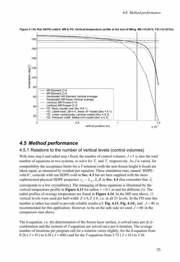
4.5 Method performance

4.5 Method performance 4.5.1 Relations to the number of vertical levels (control volumes) With time step k and radial step i fixed, the number of control volumes 1+J is also the total number of equations in two systems, to solve for sT and lT respectively. As J is varied, for compatibility the acceptance limits for a T-solution (with the non-frozen height h fixed) are taken equal, as measured by residual per equation. These simulation runs, named ‘HDPE-cold-E’, coincide with run HDPE-cold in Sec. 4.3 but are here supplied with the more sophisticated physical HDPE properties βλ,,Mp Lc − in Sec. 4.4 (but remember that sλ corresponds to a low crystallinity). The managing of these equations is illustrated by the vertical temperature profile in Figure 4.13 for radius 1.0=r m and for different J:s. The radial profiles of average temperature are found in Figure 4.14. In the Mfl runs above, 11 vertical levels were used per half-width 0,0 ≥≤ ZZ , i.e. in all 21 levels. In the FD runs this number is rather too small to provide reliable results (cf. Fig. 4.13, Fig. 4.14), and 40=J is recommended for this application. However, to be on the safe side we used 80=J in the comparison runs above.

The h-equation, i.e. the determination of the frozen layer surface, is solved once per (k,i)-combination and the systems of T-equations are solved once per h-iteration. The average number of iterations per program call for a solution varies slightly, for the h-equation from 8.26 ( 10=J ) to 6.58 ( 600=J ) and for the T-equations from 3.73 ( 10=J ) to 3.36

55

4.5 Method performance

( 600=J ). For each T-iteration an iterative T-step routine is called. However, the standard Newton step length 1.0 is directly accepted in most cases – for 10=J the T-step routine is called 8 times (out of 115 403 T-iterations overall), for 20=J 2 times (out of 108 496) and for 40=J 1 time (out of 95 758), and otherwise not at all. In all these exceptional cases the remaining residual sum, squared, is close to the acceptance limit of a solution, and neither a step length reduction nor (with one exception) the backup routine steepest descent provides improvements. All these difficulties occur at the inlet )1( =i , where the idealized initial/boundary conditions – (IC/BC) IT constant across the cavity gap, and (IC) ET constant in the wall – form a challenge. However, the overall method works also in these cases, by reducing the h-step length (closer to the solution of the previous time level k-1). The full distributions of iterations are shown in Figure 4.15. As for the h-computing, 1 iteration per program call corresponds to Hh = .

The computing time increases by J from around 11 sec. ( 10,84 == JK ) via 20 sec. ( 40,84 == JK ) to 3 min. ( 600,84 == JK ) on a 32-bit 600 MHz Pentium-3 PC, i.e. slower than proportionally to J.

4.5.2 Wall series solution We have varied the number N of wall series terms as well. In run HDPE-warm 20=N is enough to describe the temperature and frozen layer profiles for the inner cavity half ( 2.0≤r m), while at least 40=N is needed further out ( 2.0≥r m). This is due to the worsened convergence properties at the front – cf. Sec. 3.2.5. Another possibility is to decrease the time step at the very front: we have used 9.0=pTCrit (cf. Flowchart 3.1), i.e. a reduction by at most 10% per time step of the temperature difference solid melt – wall.

4.5.3 Control volume at the frozen layer Let jh denote the axial index value of the last liquid node, locally. Our original idea was to surround a movable node at the frozen layer position hz = by a control volume of vertical extension )](),([ 12

121

+++∈ jhjh zhhzz , i.e. of fixed length as long as jh is fixed, and to exclude that volume from the system of temperature equations (since the temperature is prescribed at h as MT ). However, each time h changes jh -value the total weight of the frozen layer equations changes discontinuously, which might imply that the computed residual of the h -equation (3.13), discretized, becomes discontinuous as well. In fact, in one of the runs, HDPE-cold, 1722 h -iterations out of 9766 had one non-decreasing LHS-term in the h -equation as a function of h , and the number of h -iterations were almost twice that of our final choice; where we simply exclude the volume surrounding h , letting the neighbour volumes, which surround jhz , 1+jhz , have one boundary at hz = . For this choice only 14 out of 42040 h -iterations in all four comparison runs had one of the three LHS-terms of the h -equation non-decreasing, and in none of them this unexpected behaviour (cf. Sec 3.2.3) meant a non-decreasing LHS.

56

4.5 Method performance

57

4.5 Method performance

58

5.1 Special modelling: Geometry

5 Application: Triangular plate This Chapter documents the second application type, polygonal star shaped cavities (relative to the inlet), of constant gap width. For the radial flow assumed, the distance along a stream ray to the cavity wall is crucial for the time when the streaming phase ends and the stagnant phase begins, for the ray in question. The geometry needs to be taken into account for the determination of each time step, based upon the active flow angle, the additional filled area and the gap width. This is done in Sec. 5.1. In Sec. 5.2 we describe the data and model-ling of a concrete application, a uniform triangular plate. Materials data for one amorphous thermoplastic, a polystyrene (PS), and one semi-crystalline material, a polyoxymethylene (POM), come from the data base of Cadmould, a FEM-program of Simcon. We have made a somewhat critical comment about the Cadmould viscosity and enthalpy models. As a simplifying option in Cadmould, the metal mould has not been explicitly modelled (by [Nilsson]). To match this we assume a constant depth of the cooling lines from the cavity wall surface. In Sec. 5.3 the comparison runs, two of each material, are analysed. The Cadmould runs are performed by [Nilsson]. We have to report fatal problems in the FD runs of POM, and limit the discussion to the PS runs. To compensate for our (perhaps too) strict subdivision into rays of full stream intensity and rays of complete stagnation we mention the possibility to use effective instead of nominal flow angles. The symmetry of the uniform triangle defines, e.g. three equivalent corner rays and three equivalent mid-side rays. This and the expected symmetry between the upper and lower halves of the cavity gap are used in plots of the vertical temperature profile vs. radius and vs. angular deviation from the nearest corner ray. The radial profile of the frozen layer surface (of no-flow temperature) is also evaluated. Sec 5.4 includes a few com-ments about the method performance. Apart from the iteration statistics we are also evaluating the square-root increase by time of the frozen layer. Furthermore, our velocity model has been applied to plot the time of injection for different material points at the end of filling.

5.1 Special modelling: Geometry The mould cavity is here assumed to be star shaped relative to the inlet – positioned at 0=r of a polar ),,( zr ϕ coordinate system – and the vertical cavity width is constant H2 , with symmetry plane 0=z . By the principle of the distance model and the corresponding energy principle all node points of equal flow history are equivalent as to velocities and temperatures. This means that all node positions ),( ϕr of a common radius r (equal activation time actt ) are equivalent during the streaming phase, but equivalence during the succeeding stagnant phase also requires a common distance to the mould wall along the radial flow directions (equal stagnation time stagt and thus equal residence time of the fluid). As input the vertical boundary planes of the cavity are specified by the consecutive ),( yx - corner positions. For a computation of stagt , as well as active flow angle actϕ and the filled volume, the geometry needs to be taken into account.

Since the mould cavity has constant gap width, the fluid expansion is viewed as an essentially 2D-space process in a flat, polygonal domain X. Consider a boundary line of X. Its intersection L with X is specified by the two corner points a, b − endpoints of the line segment L – and given by ( , ), ( , )r ra a b bϕ ϕ where ϕ ϕb a> is assumed. In the star shaped domain, L occupies a positive sector angle ϕ ϕb a− as viewed from the injection point at the origin. The region

59

5.1 Special modelling: Geometry

enclosed by L and its two endpoint radii is a triangle T, and X is a union of such triangles.

Consider for a moment a basic boundary line, written in parameter form

x t x t x x x xy t y t y y y y

a b a

a b a

( ) , :( ) , :

= + ⋅ = −= + ⋅ = −

∆ ∆∆ ∆

where ( , ), ( , )x y x ya a b b are the endpoints of the line segment L, which has the length

22 )()(: yxdab ∆∆ += . The boundary line point ( ( $), ( $))x t y t closest to the injection point at the origin is determined by

2:ˆab

aa

dyyxx

t∆∆ ⋅+⋅

−=

and its distance from the origin is

ab

aa

dxyyx

r∆∆ ⋅−⋅

=:ˆ .

Denote by r0 the distance of L from the injection point; whence $, $r t determine

rr tr ra b

0

0 1:

$ $ ( , )min[ , ]

=∈

otherwise.

Now let r denote a front circle radius of the expanding fluid. For a mathematical description of the part of T covered by fluid, four cases are distinguished during the filling process.

1. Before the front reaches L, i.e. as 0rr ≤ , the covered part of T is a circle sector of area

π ϕ ϕπ

ϕ ϕr rb a b a2 2

2 2⋅

−= ⋅

−.

2. When the front intersects L at two points ( , ), ( , ),r rϕ ϕ ϕ ϕ1 2 2 1> , i.e. as the point on L closest to the origin lies between its endpoints and ],min[0 ba rrrr << , one triangle in the middle plus two surrounding sectors contribute to the area

r

r b a2

2 1 2 2 1

2 2⋅ −

+ ⋅− + −sin( ) ( ) ( )ϕ ϕ ϕ ϕ ϕ ϕ

.

3. When the front intersects L at one point ( , )r ϕ , i.e. as min[ , ] max[ , ]r r r r ra b a b< < , fluid covers L from one endpoint up to the point of intersection. The covered part of T is a triangle plus a sector, of area

. casein

22)sin(

, casein 22

)sin(

2

2

baabb

babaa

rrrrr

rrrrr

<−

⋅+−⋅

>−

⋅+−⋅

ϕϕϕϕ

ϕϕϕϕ

4. When the fluid covers L completely, i.e. as r r ra b≥ max[ , ] , all of the triangle T is filled area

r ra b b a⋅ −sin( )ϕ ϕ

2.

60

5.2 Materials data

In these cases only the circle sector parts contribute to the active front at r. Their angular sum is the overall active flow angle ϕ act r( ) . For a point ( , )x y T∈ , at a distance r( )> 0 from the injection point at the origin, the stagnation time ),( yxtstag is when the flow radius through ( , )x y reaches L:

).1(:, ≥⋅−⋅⋅−⋅

=⋅=yxxyyxxy

rr aastag ∆∆

∆∆ββ

During time step No. k, when the radius of the front circle expands another r∆ , the additional covered polygonal area ∆Ak is obtained by summing up T-areas, and – in consideration of the efficient local gap width h – the time step ∆t k etc. can be determined as in Sec. 4.1.1.

5.2 Materials data Simulation runs for comparison have been performed by [Nilsson], using the commercial software Cadmould of Simcon, Fill version 1.110. In the concrete application, X in Sec. 5.1 was chosen as an equilateral triangle, with the inlet almost in the middle (4 mm from the centroid). From the Cadmould (“Cmd” below) data base of standard materials, one amorphous thermoplastic – the polystyrene Polystyrol 158 K of Basf AG (“PS” below) – and one semi-crystalline material – the polyoxymethylene Delrin 100 NC-10 of DuPont (“POM” below) – were (arbitrarily) chosen. One run of normal processing conditions (“fast” below) and one of slow filling (“slow” below) were simulated for each material. The triangle sides were chosen extreme (60 cm) to provoke freezing. The plate thickness is 2 mm. The comments below on Cmd are solely based upon these four simulation runs. According to the materials documentation, the Cmd model assumes constant heat conductivity, constant diffusivity and the existence of a no-flow temperature. These temperatures deviate a lot from the reported melting point C 178 o=MT for Delrin (DuPont product information, www.dupont.com/ enggpolymers) and from the glass transition temperature C 100 o=GT for Polystyrol (MatWeb, www.matweb.com). The latent heat of crystallization seems to be neglected. The density variations are described by a Carreau PVT model – cf. [Kennedy], p.28-29. The viscosity obeys a model of T , γ& that includes 2 universal and 5 material specific parameters, according to [Kutschera] – for Delrin see Figure 5.1, which we have constructed from the Cmd input data. Here the overall increase by T for fixed γ&ln is indeed questionable. However, for comparison we have adjusted the FD Arrhenius parameter of η in a best-fit estimation procedure to this questionable behaviour. In Table 5.1 all materials data of the simulation runs are collected, together with our fitted parameters, marked by asterisks. Our FD densities are estimated from the Cmd PVT model, and our heat capacities are then determined by the given diffusivity values.

In the Cmd runs, as a simplifying option, the metal mould has not been explicitly modelled. According to [Kutschera], the contact temperature at the inner wall surface is computed from standard wall conductivity and diffusivity, and prescribed wall temperature. The exact model is unknown to us. To match that model we have used the standard Moldflow mould wall parameters – see Sec. 4.2 – and have applied a constant depth of the cooling channels,

9=WH cm, the rounded average in the Moldflow runs.

61

5.2 Materials data

Table 5.1 Materials data used in basic FD runs

Polystyrol 158 K Delrin 100 NC-10

1015* 1240*

1045* 1320*

0.14 0.158

1473 2708

1517 2883

445.74* 316352*

2005.2* -184.76*

-273.2 141.79*

0.24836* 0.37405*

--- 0

130 153

lρ

sρ

sλλ =l

LH

01)/(

0 KeK nTTB B −− ⋅⋅= γη &

B

n

3kg/m3kg/m

BT

nsPa ⋅

spc ,

l,pc

flownoT −

Co

Co

CoJ/kg

CW/m o

CJ/kg o

CJ/kg o

62

5.3 Comparison runs

5.3 Comparison runs

5.3.1 Average temperature The Cadmould (Cmd) runs assume “pressure-controlled filling 99%”. Since no explicit pressure bound seems to be prescribed, we interpret this as if the pressure registered at the inlet, when 99% of the cavity volume is filled, is dimensioning and is kept constant throughout the rest of the filling phase. In practice this means a successive reduction of the final flow rate. During the first 99% of filling a constant flow rate is applied, chosen to provide the prescribed 99%-filling times 2.006 s (run PS-fast) and 8.000 s (run PS-slow), respectively. This causes big differences between the runs in resulting temperatures – see Figure 5.2 for a general view of the final average temperatures in our FD runs, presented on one and the same colour scale. The steep temperature rise at the corner rays are subject to several comments below. If the nominal residence times, computed in the absence of freezing and for a plug-formed rv -velocity profile, were decisive to the result, the coldest regions would be along the triangle sides, and there would be no reversing of temperatures along any stream ray from the inlet and outwards.

Both our FD runs on the high viscosity POM Delrin have failed: In run POM-slow, although our FD method works, the vertical temperature profiles are characterized by a narrow peak of extremely high temperature (and viscous energy), originating in the last second of filling simulation. In run POM-fast the Jacobian matrix G in Sec. 3.3.2 becomes ill-conditioned (by

0<B ) and the backup routine is not sophisticated enough to provide acceptable convergence from the chosen starting point. Since the temperatures even in run POM-slow of Delrin become non-physically high, we have not worked on improving our method to handle run POM-fast as well. A plausible explanation for the failure is the non-physical Cmd viscosity model for this material – see Fig. 5.1 – also remaining in our model – see Tab. 5.1, where the negative B-value indicates that the viscosity increases by temperature. Since the volume flow rate is prescribed, the high 0K -value causes high viscous energy levels and correspondingly high temperatures, which add to the viscosity instead of acting as the ordinary stabilizing mechanism. The severity of these extreme input data is reinforced by the shortcomings of our model as discussed below, revealed as the flow sectors are narrowing. For these reasons we will limit our discussion to the two PS-runs. A Cmd result data file documents the state at the end of filling, as to pressure, temperature, shear stress, velocity and frozen layer. According to the Cadmould file name convention, the whole filling phase takes 2.054 s in run PS-fast and 8.368 s in run PS-slow. Our corresponding times are 2.082 s and 8.277 s, respectively. The time deviations are attributed to pressure differences. The Cadmould pressure data indicate final levels at the inlet around 650 bar in run PS-fast and 800 bar in run PS-slow. These are contradictory to our interpretation of “pressure-controlled filling 99%”, both as to magnitude and relation: Our dimensioning 99%-pressures become 1177 bar in run PS-fast (after 2.005 s) and 1027 bar in run PS-slow (after 8.011 s). As for relations, a higher pressure level is expected in run PS-fast than in run PS-slow due to the higher flow rate. As for the pressure magnitudes, we see some weaknesses of our distance model, where the active flow angle concept (cf. Sec. 5.1) assumes rigid boundaries between streaming and stagnant fluid. In practice we would expect these boundaries to be flexible, admitting some tangential outflow to the stagnant sectors close to the inlet in a high-pressure situation and compensated by tangential inflow ahead of the flow

63

5.3 Comparison runs

front. We might instead use the term effective flow angle to describe these phenomena. As an illustration, see Figure 5.9 below for “run PS-fast-E”, which denotes run PS-fast with the addition of a 10 o flow angle, whenever possible, to each side of every active flow sector in the FD run, i.e. the overall effective flow angle is 60 o ))1010(3( +⋅= more than the nominal angle at the end of filling. Fig. 5.9a-b should be compared with Fig. 5.3a and Fig. 5.4c, respectively – see comments below. The final pressure at the inlet in FD run PS-fast-E is 901 bar, and the filling takes 2.039 s. We have not developed the concept effective flow angle further, but it might be relevant also in case of non-star shaped cavities, where flow around corners causes singularities, if the strict distance model is applied.

The vertical average temperatures, computed for different node positions ),( ϕr at the end of filling, are presented in Figures 5.3-5.6, where Fig. 5.3-5.4 refer to run PS-fast and Fig. 5.5-5.6 to run PS-slow. The plot symbols for the Cmd values differentiate between cavity nodes at the upper wall surface 1+=z and at the lower surface 1−=z . Due to triangular symmetry, nodes of equal r and equal −ϕ deviation from the closest corner ray (from inlet to triangle corner) are equivalent as to temperatures, etc. The −ϕ deviation 0 o corresponds to nodes on a corner ray – the three final flow directions – and 60 o refers to nodes on a midside ray – the three directions of first stagnation. In Fig. 5.3, 5.5 the node rays are grouped into 3 o −ϕ deviation classes, of which a subset is presented. Especially in run PS-slow there are extreme differences – more than 100 Co near the inlet – between the Cmd temperatures registered for the 1+=z -and 1−=z -nodes, respectively. According to [Kutschera] both are average nodal values from wall to wall ( 11 +≤≤− z ). Even if the vertical positions are weighted differently for the two node groups and if the implicit Cmd cooling model handles the upper and lower part differently, we have no obvious explanation for such big differences. Notwithstanding this big temperature span of Cmd, our FD temperatures show systematic deviations. In Fig. 5.3a all nodes close to the corner rays are plotted. Our FD temperatures are higher, except at the inlet )0( =r and at the mould wall )m 35.0( ≈r . For each plot in Fig. 5.3 the FD temperatures fall in relation to the Cmd temperatures – except at the mould wall. The same phenomenon appears for the six radial classes in Fig. 5.4a-e, where the Cmd temperatures decrease much slower tangentially, from the final flow direction

)0deviation-( o=ϕ to the direction of first stagnation )60deviation-( o=ϕ . The overall average fluid temperatures Cmd-FD coincide, 187 Co . In run PS-slow, Fig. 5.5-5.6, the overall average temperatures differ, 132 Co for FD and 139 Co for Cmd. When the strict distance model is applied in run PS-fast, we contribute some of the discrepancies to our above mentioned negligence of tangential convection, to which our negligence of tangential conduction should be added, together preventing any tangential temperature levelling. On the other hand, an increased steepness near o0deviation- =ϕ is expected due to finally accele-rating shear rates, instead of the levelling out that the Cmd temperatures show in Fig. 5.4.

64

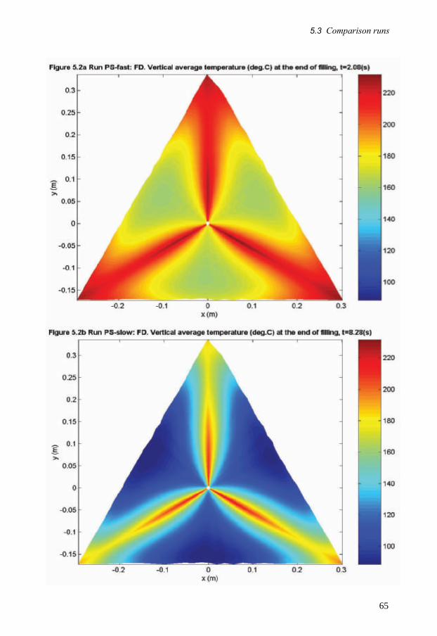
5.3 Comparison runs

65

5.3 Comparison runs

Figure 5.3 Run PS-fast: Cmd and FD. Vertical average temperatures at the end of filling. Rays of different −ϕ deviations, measured from the closest corner ray.

66

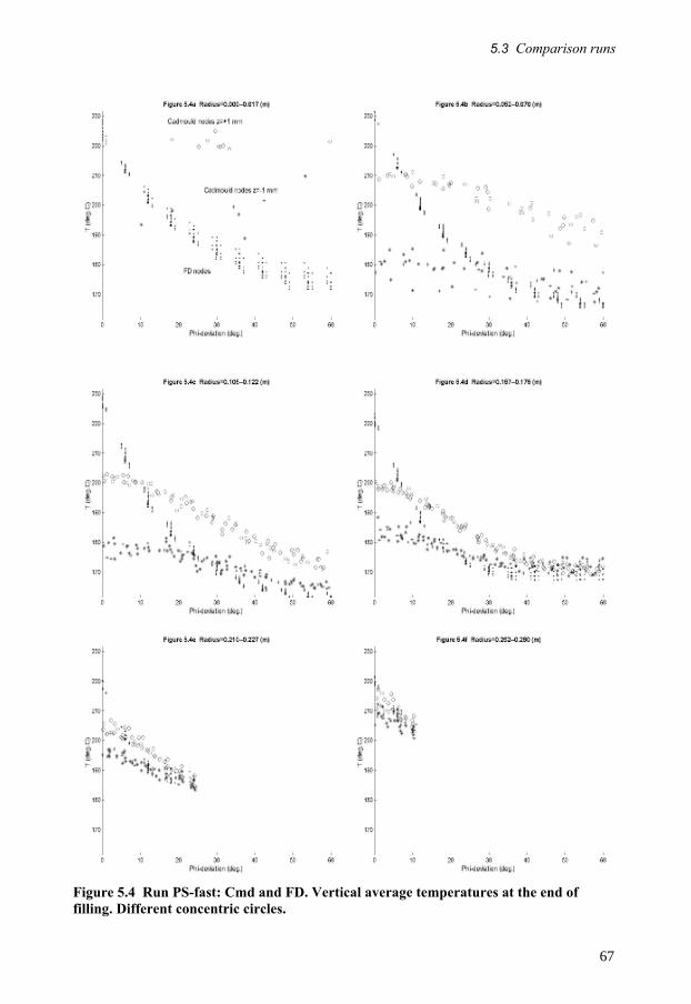
5.3 Comparison runs

Figure 5.4 Run PS-fast: Cmd and FD. Vertical average temperatures at the end of filling. Different concentric circles.

67

5.3 Comparison runs

Figure 5.5 Run PS-slow: Cmd and FD. Vertical average temperatures at the end of filling. Rays of different −ϕ deviations, measured from the closest corner ray.

Figure 5.6 Run PS-slow: Cmd and FD. Vertical average temperatures at the end of filling. Different concentric circles.

68

5.3 Comparison runs

69

5.3 Comparison runs

70

5.3 Comparison runs

Figure 5.9 Run PS-fast-E: Cmd and FD (effective flow angle: +60 o ). Vertical average temperatures at the end of filling. (a): rays of similar −ϕ deviations, measured from the closest corner ray, (b): concentric circles of similar radius.

5.3.2 Temperature profiles In Figure 5.7a-b we illustrate the temperature contrast at the end of filling in run PS-slow, between two flow directions – a corner ray is shown in Fig. 5.7a and a midside ray (where the fluid hits the wall after 4.83 s) in Fig. 5.7b. One and the same colour scale is used. In Fig.5.7b part of the fluid is frozen to the bottom, in Fig. 5.7a we recognize the frozen layer profile from Ch. 4, with the maximum layer thickness far from the inlet. In Figure 5.8a-b we con-sider the time evolution of vertically registered temperatures, at two nodes chosen on a corner ray. At the inlet – see Fig. 5.8a – a thin frozen layer is built up initially, but towards the end of filling the increased pressures, velocities and shear rates make the layer melt. At 9.5 cm from the inlet– see Fig. 5.8b – the same kind of evolution is even more pronounced – two thirds of the layer that exists at 5.05 s are molten at the end of filling. (This phenomenon, but far more extreme, is decisive for our Delrin simulation failures. Realistic or not: our model behaves like this when the flow is confined to narrowing flow sectors.) The final temperature rise is also traced as the hot spot in Fig. 5.7a. This is also an explanation for the slow fall of the FD average temperature in Fig. 5.5a (run PS-slow) and for the initial rise by radius in Fig. 5.3a (run PS-fast). Comparisons with the Cmd frozen layers in run PS-fast for all nodes in two ϕ -deviation classes are shown in Figure 5.10a-b below. The Cmd bottom layer is much thicker than the top layer, for unknown reasons, if not for the implicit cooling. As can be seen in Fig. 5.10a for the corner rays, the Cmd maxima at the lower and upper walls occur at a smaller radius than the corresponding FD value. There is a systematic change of FD maximum position and value as the ϕ -deviation angle increases, while the Cmd maxima are essentially constant – both as to radial position and, especially at the lower wall surface, as to extension. Before the (local) time of stagnation the relative, rather than the absolute, position along a flow line is expected to be decisive for the maximum. At the end of filling a tangential heat flow, which we completely ignore, might have accomplished some levelling, but the almost full angular symmetry of the Cmd frozen layers is hard to understand.

71

5.4 Method performance

5.4 Method performance

5.4.1 Square-root parameter To predict the frozen layer thickness hH −=δ after a new time step, a acttt − -increase (cf. Sec. 3.1.3) is optional in our simulation program, both for the streaming fluid and in the stagnant regions. For the streaming fluid in run PS-fast this option does not perform better than to start the h-iterations (h is the non-frozen height) from the previous value, without extrapolation. A glance at Fig. 5.8 explains this, since the normal increase during the first seconds is followed by a shrinking layer. In run PS-slow a 50-50-weighted combination of the latest square-root coefficient, computed as acttt −δ , and the previously registered average coefficient performs better. In the stagnant phase the growth rate (faster) differs radically from that of the streaming fluid. Therefore a node specific, equivalent activation time actt is estimated initially and used thereafter. By extrapolating the latest registered expansion rate, according to the square-root formula, a few percent of the h-iterations are saved.

5.4.2 Iteration statistics Since the stagnant phase, for fixed h and with constant parameters, represents linear systems of equations in each phase, liquid and solid, we expect the Newton temperature iterations to converge in one step to the solution. This is accomplished – always with step length 1 – if we avoid applying an upper limit of accepted temperature changes per iteration; which is used in the nonlinear case. The average number of iterations per program call, for the computation of a new h-solution (for fixed node and time), is the same as in Ch. 4 (with nonlinear viscosity and temperature dependent parameters): 6.31 h-iterations per call in the streaming phase and 6.73 in the stagnant phase for run PS-fast. The rather tough convergence criterion used, with an overall residual squared sum ff TF = below 1210− for 80=J vertical node levels, is no problem. Stop values in Flowchart 3.1 are 1410665.1 −⋅=FTEps , 510−=FhEps and

8103.51_ −⋅=hEps . The whole run, with extensive checking and saving on files, takes a few minutes if 84=K time steps (radial levels), 20=uPhi nodes per radial level and 80=J are used.

5.4.3 Velocity profiles and residence time In this application we have used two terms only in the power series expansion of viscosity and velocity components. Apart from the isothermal exponent n

11+ in (3.4), the estimated exponent of the additional term always becomes n

13 + . The velocity components can be used for computing the residence time, or equivalently, the time of injection for the stagnant fluid at the end of filling. In Figure 5.11a the vertical average time of injection is shown for the triangle, in Figure 5.11b the vertical distribution is plotted for a corner ray. Due to the hot, fast moving material at the centre plane, redirected vertically at the front, and to the freezing followed by melting as the shear rate increases at the walls, the pattern becomes complex. Fig. 5.11a can be compared with Fig. 5.2a. The distributions of residence time (time of injection) and the average temperature are similar, although both show a non-standard behaviour, influenced by local freezing and succeeding melting.

72

5.4 Method performance

73

5.4 Method performance

74

6 Conclusions

6 Conclusions In the two implemented radial flow applications the plus points for our FD program are:

• It admits variable material properties of both melt and metal mould (Sec. 2.2, 3.2.5).

• It can be run with material and process input data similar to those used in commercial programs.

• Some interaction between the momentum and energy equations is considered by an analytical pressure-velocity model, fitted to FD-computed temperatures via a linking viscosity (Sec 3.1).

• Fairly realistic temperature profiles in Fig A1.1 (cf. Fig. 4.9) indicate that our analytical link with the pressure-velocity fields replaces a FEM model reasonably well. The stable velocity profiles in Fig. A1.1 support our approximation by a common profile along the flow ray.

• It takes full advantage of the symmetries, streaming fluid being handled by a single flow ray and stagnant fluid by one representative for each node group sharing flow history.

• We use the possibilities to simplify the basic PDE in regions of stagnant fluid and in cavity parts of “solid”, “frozen” fluid.

• The axial node spacing can be chosen non-uniform, adjusted to a steeper temperature variation at the cavity wall, without jeopardising the numerical accuracy (Sec. 3.3.1).

• The resulting nonlinear systems of FD-equations are small, efficiently solved on a standard PC.

• For realistic materials our solution method is reasonably robust, being supported by theoretical and practical convergence results (Sec. 3.2, 3.3.2, 4.5, 5.4).

• The qualitative agreement FD - Mfl (Moldflow) and FD - Cmd (Cadmould) is acceptable/good, as a rule, both for pressure evolution (Fig. 4.5) and temperatures (Sec. 4.3.2, 5.3.1).

In the comparison runs with the two commercial FEM-FD programs we notice big temperature differences in two cases:

• At the flow front (FD - Mfl). We refer this to different PDE-formulations of axial heat flow (Sec 2.3.3 and [Kennedy], p.71). Our two front models, conventional convection and fountain flow (cf. Fig. 4.8), are unanimous in this respect, and we claim they are realistic.

• In narrow flow sectors (FD - Cmd). We explain this by our negligence of angular convection and conduction. The discrepancy is fatal for a material with unrealistic viscosity dependence upon temperature. Although our FD-method converges in one such run, the rapid temperature rise in the diminishing flow sectors is unrealistic An isothermal viscosity model would perform better here but worse on realistic material models. Our decisive model weakness is an exaggerated shear rate (Sec. 5.3.1).

75

6 Conclusions

As for the commercial programs we are critical in some respects, with reservations for our limited study and insight:

• Some basic material data and some modelling methods show questionable quality: different values are found in different data bases, and unrealistic data are indiscriminately used (Sec. 4.2, 5.2, 5.3.1).

• The realism of some parts of the material model might be improved: the viscosity model should rely on known asymptotic results and – according to our findings in Sec. 4.4 – also allow pressure-dependence, and the material model should admit temperature-dependent thermal conductivity, specific and latent heat. (However, we have not set an example, in relying on the power-law behaviour with fixed index n.)

• The asymmetry between the upper and lower cavity halves is in some cases extreme, for unknown reasons (Fig. 4.9-10, 5.3-6).

• The axial heat convection, especially at the flow front, should not be ignored (Mfl; the Cmd model is unknown to us).

• The angular stretching part of the shear rate should not be neglected in radial flow (Sec. 2.3.3 and [Kennedy], p.70).

Some observations of the general filling process are:

• Our radial temperature profile takes its minimum and the frozen layer is thickest closer to the inlet than suggested by Mfl (FD - Mfl: Fig. 4.8, 4.10). We consider this to be an implication of the different axial heat models at the front.

• The axial temperature profiles and the frozen layer thickness show non-monotone evolution by time (FD: Fig. 5.11b). We explain this by local viscous heating and melting caused by increased shear rates in narrowing flow sectors. (Hence our effect might be somewhat exaggerated.)

Our main experience and insight is:

• As for the narrow flow sectors, in relying on the commercial program Cmd, we must admit the shortcomings of the distance model and our 2D heat flow principle, even in a triangular case (cf. Fig. 5.4). Although we have mentioned the possibility to modify our principle (by the concept of an effective flow angle, Fig. 5.9), such a modification is hard to implement in a general case. In this sense our 2D temperature model fails to be equally robust as the distance model itself. For educational purposes, on the other hand, even a 2D FD-model is too sophisticated to balance the simplicity of the distance model.

• As a by-product we have formulated two different analytical forms of temperature solutions – see App. 1-2 – based on our pressure-velocity model and on an extended Stefan problem, respectively. These or similar classes of temperature profiles are hopefully robust, e.g. in narrow flow sectors and in complex geometries, simple enough to be transparent and yet capture the main variation. In the development of such standard profiles our FD program might be of some value.

76

References

Advani, S.G. (ed.), Flow and Rheology in Polymer Composites Manufacturing, Elsevier, Amsterdam, 1994. Agassant, J.-F. et al, Polymer Processing, Munich, 1991. Ames, W. F., Nonlinear Partial Differential Equations in Engineering, vol. I, Academic Press, New York, 1965. Aronsson, G., On p-harmonic functions, convex duality and an asymptotic formula for injection mould filling, European J. Appl. Math. 7 (1996), 417-437. Baehr, H.D. and Stephan, K., Heat and Mass transfer, Springer, Berlin, 1998. Baird, D.G. and Collias, D.I., Polymer Processing, Butterworth-Heinemann, Newton, MA, 1995. Becker, J., Berggren, K., Nilsson, L.-Å., Strömvall, H.-E., Formsprutningsteknik, Yrkesnämnden för fabriksindustrin (YFIND), Stockholm, 2000. Berins, M.L. (ed.), Plastics Engineering Handbook of the SPI, 5th ed., Chapman & Hall, New York, 1991. Bicerano, J., Prediction of Polymer Properties, Dekker, New York, 1993. Birkhoff, G. and Rota, G.-C., Ordinary Differential Equations, John Wiley, New York, 1989. Carslaw, H.S. and Jaeger, J.C., Conduction of Heat in Solids, Oxford Univ. Press, Oxford, 1959. Dennis, J.R. & Schnabel, R.B., Numerical methods of unconstrained optimization and nonlinear equations, Prentice-Hall, Englewood Cliffs, NJ, 1983. Gustafsson, B., Kreiss, H.-O. and Oliger, J., Time Dependent Problems and Difference Methods, Wiley, New York, 1995. Hieber, C.A. and Shen, S.F., A finite-element/finite-difference simulation of the injection-molding filling process, J. Non-Newtonian Fluid Mech. 7 (1980), 1-32. Holman, J.P., Heat Transfer, McGraw-Hill, New York, 1997. Horn, R.A. & Johnson, C.R., Topics in matrix analysis, Cambridge Univ. Press, Cambridge, 1991. Isayev, A.I. (ed.), Injection and Compression Molding Fundamentals, Dekker, New York, 1987. Johansson, P., On a Weighted Distance Model for Injection Moulding, LiU-TEK-LIC-1997:05, thesis No. 604, Linköping, 1997. Kennedy, P., Flow Analysis of Injection Molds, Hanser, Munich, 1995. Kutschera, H., (Personal comm.), Simcon kunststofftechnische Software GmbH (producer of Cadmould). Manzione, L.T. (ed.), Applications of CAE in Injection Molding, Hanser, New York, 1987. Meyer, C.D., Matrix Analysis and Applied Linear Algebra, SIAM, Philadelphia, 2000. Morton-Jones, D.H., Polymer Processing, Chapman & Hall, London, 1989. Nilsson, L.-Å., (Personal comm.), PolyInvent AB (distributor of Cadmould in Sweden). Ortega, J.M., Matrix theory, Plenum Press, New York, 1987. Ortega, J.M. and Rheinboldt, W.C., Iterative Solution of Nonlinear Equations in Several Variables, Academic Press, New York, 1970. Pearson, J.R.A., Mechanics of Polymer Processing, Elsevier, Barking, Essex, 1985. Perepechko, I., Low-temperature Properties of Polymers, Mir, Moscow, 1980. Rao, N.S., Design Formulas for Plastics Engineers, Hanser, Munich, 1991. Renardy, M. and Rogers, R. C., An Introduction to Partial Differential Equations, Springer, New York, 1993.

77

Siginer, D.A., DeKee, D. and Chhabra, R.P. (ed.s), Advances in the Flow and Rheology of Non-Newtonian Fluids, Part B, Elsevier, Amsterdam, 1999. Smith, G.D., Numerical Solution of Partial Differential Equations: Finite Difference Methods, Clarendon Press, Oxford, 1985. Storck, K., Thermal system analysis: heat transfer in glass forming and fluid temperature-control systems, LiU dissertation No. 542, Linköping, 1998. Straughan, B., The Energy Method, Stability, and Nonlinear Convection, Applied Math. Sciences 91, Springer, New York, 1992. Strikwerda, J. C., Finite Difference Schemes and Partial Differential Equations, Wadsworth, Belmont, CA, 1989. Tadmor, Z. and Gogos, C.G., Principles of Polymer Processing, Wiley, New York, 1979. Tucker, C.L. (ed.), Fundamentals of Computer Modeling for Polymer Processing, Hanser, Munich, 1989. Valtonen, M.., (Personal comm.), Tampere University of Technology, Institute of Materials Science, Plastics and Elastomers Technology. Van Krevelen, D.W., Properties of Polymers, Elsevier, Amsterdam, 1990. Özisik, M.N., Finite Difference Methods in Heat Transfer, CRC Press, Boca Raton, Fda, 1994.

78

Appendix 1 Vertical velocity profiles As one example, consider (3.1) with the special choice

2

431:

⋅−=

hz

hzg for hz ≤|| , Hh ≤ . The

viscosity increases as hz ↑|| by the factor 1−nγ& and here, due to the temperature gradient, also by the factor )/( BTTBe − . The no-slip boundary condition 0)( =hV implies

n

nn

nn

nnnnn

chzc

hzczV

41

25

113

1431

1

)4)(2(,1

31

1)(

11111

+++

=

−

+−

−

+=

++

;

corresponding to the two leading terms of the series expansion (3.4). The velocity profile becomes less plug-like than for the isothermal case – see Figure A1.1a. Unlike the isothermal case, maximum shear rate does not occur at the very no-flow boundary, but inside (cf. [Manzione], p.259, and [Pearson], p.610). A corresponding temperature profile, based upon (3.2), is illustrated.

As a second example we choose 3

411

2

21:

⋅−

⋅+=

hz

hz

hzg – see Figure A1.1b. Although the

velocity profiles in Fig. A1.1a,b are quite similar, the temperature profiles differ a lot – cf. the assumption in Sec. 3.1.1 of a common V(z) and the temperature profiles in, e.g., Fig. 4.9.

79

Appendix 2 Further comments on the Stefan problem A2.1 Freezing layer in the presence of particular heat generation In our FD-implementation we use the square-root model of the frozen layer expansion )(tδδ = to estimate both the time evolution in the filled region and, optionally, the initial temperature profile at the flow front. These estimates are based upon the formulas in Sec. 3.1.3. In this Appendix we will describe two possible improvements of the temperature estimates. As it happens the first extension to a high extent captures the decreasing frozen layer thickness towards the inlet in a radial flow situation, unlike the standard square-root model (cf. [Carslaw & Jaeger], p.282). Here we extend the 1D Stefan problem of Sec. 3.1.3, by considering internal heat generation ),( tzQ per unit volume and time, imitating local convection and dissipation. (The horizontal position x, y is fixed.) It is reasonable that the square-root behaviour of tt sκεδ 2:)( = remains for a certain class of generation functions. The z-axis is here reversed, so that one-dimensional heat conduction is in the opposite z-direction, i.e. the wall surface corresponds to z=0 and the mould gap is the semi-infinite medium

0>z . Let t

zyc s

ll κκκ

4:,:3 == , where phase region l corresponds to )(tz δ> , i.e. ε3cy > .

In the solid region )(0 tz δ<< , let the BC at the wall surface z=0 be 00 ≡,t)(Ts . In the liquid region the PDE is written

.),(1)(2

2

l

l

l

l

ll

ll

λtzQ

tT

zT

tzT s −=

∂∂

⋅−∂

∂⋅′⋅

−+

∂∂

κδ

κρρρ

The 2nd term on the LHS corresponds to the convective term in PDE (3.11), with zv according to

(3.10), where ,0≈∂∂

rh 1)1(~)~(~ =≈ UzU is assumed. As for the BCs at the layer surface )(tz δ= and at

∞→z , see [Carslaw & Jaeger], p.284. We make a separable-solution ansatz )()( tgyD ⋅ . For the three PDE-terms on the LHS to have a common t-factor we must have ttgtg )()( ⋅=′ α , i.e. αttg ⋅= const)( , α arbitrary, and ( ) 14:),( −⋅= ακ ttzftzQ l . Let

α

κt

t

zDtzUtzT ⋅+=

l

l4

),(:),( ,

where U satisfies the corresponding homogeneous PDE in the liquid region and takes care of the BC at infinity, and )(yD for ε3cy ≥ solves the inhomogeneous ODE

ll ,

232124:,)(:),()(4)()1(2)(

PcDccDyfDyDyDDyyD

ρεα =−=−=−′++′′ .

In consideration of the time dependence of ),( tzTl upon αt – there is one BC at infinity )( ∞→z and two BCs at )(tz δ= to satisfy when t varies – 0=α is necessary for general f:s. This makes the ODE of 1st order and linear for )(yD′ – but restricts the class of generation functions to 1)( −⋅ tyf . For the assumed form )(tδ , the temperature function U for some constant B ([ibid.], p.291) satisfies

+−⋅−∞−= 1

4erf1)(:),( D

tzBDTtzU Ilκ

.

Since U for 0=α also solves the homogeneous ODE, D is taken as a particular solution determined by the initial values )( 3εcD , )( 3εcD′ (cf., e.g., [Birkhoff & Rota], p.41). A power series solution is easily obtained given a series expansion of f ([ibid.], p.99). The BC corresponding to (3.7), determining the layer expansion parameter ε , becomes

επεπ

εεε

εε

)()(2)(

)(erf-1))(exp()]()([

)(erf)exp(

,

31

2

2231

2

EMsP

M

EMEM

MI

TTcL

TTcDc

cc

TTcDTDTc

−=

−′

−−

⋅−

+−∞−⋅−

− .

80

Here the excess melting temperature (above the zero wall temperature) is denoted EM TT − .

If, instead, the wall is modelled as a separate semi-infinite region ([ibid.], p.288), then, as in Ch. 3 (cf. (3.8)), we obtain a correction by 0c in the denominator of the first term of the ε -equation.

To illustrate the function class 1)( −⋅ tyf , we consider 2

)21()( 1yeyDayf −+⋅= , 0>a , where Q

takes its maximum at tDz lκ41≈ . For all functions in the class, the overall (integrated) heat generation in }0),(|),{( filltttztz <<> δ becomes proportional to fillt . In the special case we get

2

)2/()( 2yeDayD −⋅= as the additional temperature due to heat generation. This is illustrated in

Figure A2.1a-c, for model (3.8) and its Q-extension. The relations between the a-values in Fig. A2.1a-c correspond to the viscous energy relations attributed to the different radial positions and their influence upon the average radial velocity and 1+nγ& . The time since activation is 2 s in a

)m 3.0( =r , 3 s in b )m 2.0( =r and 5 s in c )m 1.0( =r . In Fig. A2.1a we notice that already (3.8), i.e. 0=a , yields a shape similar to the FD simulated temperature profile, taken from Fig. 4.9d, but in Fig. A2.1b-c, which represent cavity parts far behind the front and behind the maximum frozen layer (cf. Fig. 4.9c-b), the Q-extended model provides better fit (especially in the frozen layer).

81

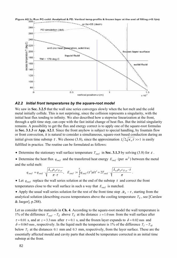
A2.2 Initial front temperatures by the square-root model We saw in Sec. 3.2.5 that the wall sine series converges slowly when the hot melt and the cold metal initially collide. This is not surprising, since the collision represents a singularity, with the initial heat flux tending to infinity. We also described how a stepwise linearization at the front, through a split time step, can cope with the fast initial change of heat flux. But the initial singularity remains. A possibility to get the flux and energy correct is to apply one of the square-root formulas in Sec. 3.1.3 or App. A2.1. Since the front anyhow is subject to special handling, by fountain flow or front convection, it is natural to consider a simultaneous, square-root based conduction during an initial given time substep τ . We choose (3.8), since the approximation 12 >>τκ wL is easily fulfilled in practice. The routine can be formulated as follows:

• Determine the stationary wall surface temperature surfT in Sec. 3.1.3 by solving (3.8) for ε .

• Determine the heat flux surfq and the transferred heat energy surfE (per 2m ) between the metal and the solid melt:

π

τρλττ

τπρλ τ ⋅

⋅=′′=⋅

⋅= ∫wPww

surfsurfsurfwPww

surfsurfc

TdqEc

qq ,

0

, 2)(:, .

• Let surfq replace the wall series solution at the end of the substep τ and correct the front temperatures close to the wall surface in such a way that surfE is matched. • Apply the usual wall series solution for the rest of the front time step τ∆ −kt , starting from the analytical solution (describing excess temperatures above the cooling temperature ET , see [Carslaw & Jaeger], p.288). Let us consider the materials in Ch. 4. According to the square-root model the wall temperature is 1% of the difference Esurf TT − above ET at the distance mm 0.1=z from the wall surface after

01.0=τ s, and at mm 3.3=z after 1.0=τ s, and the frozen layer expands to mm 02.0=δ and mm 065.0=δ , respectively. In the liquid melt the temperature is 1% of the difference MI TT −

below IT at the distances 1.0 mm and 3.0 mm, respectively, from the layer surface. These are the essentially affected mould and cavity parts that should be temperature corrected in an initial time substep at the front.

82

Wall Solid melt TE

z=H (z´=H´)

TM Tw

qw

Figure A3.1 Input/output data at series solution of wall and solid melt PDEs. Fixed h, time step k.

z=h (z´=0)

Appendix 3 Solid melt: a series solution For both the active-flow set )(tA and the passive-flow set )(tB , defined in Sec. 3.2.1, the heat balance of the frozen layer ]),,(( Hthz r∈ is controlled by one and the same conduction PDE. The interaction with the metallic mould (cavity wall) is two-way: the heat flux wq through the wall surface is a result of the wall series solution in Sec. 3.2.5, and the surface temperature – to be determined here – is an input to the wall PDE. The frozen layer IBVP has BCs MTT = at

),( thz r= and ws qzT =

∂∂λ at Hz = , and no IC, since the frozen region is an empty set at 0=t ,

and the local activation time actt satisfies Hth act =))(,( rr for all cavity positions r .

For semi-crystalline polymers with ssPs c λρ ,, , approximately independent of temperature, the PDE becomes linear and a series solution exists. For all amorphous materials below GT , the

conductivity Ts ⋅+= 10: λλλ is nearly proportional to Tccc sP ⋅+= 10, : , i.e. 0:0

1

0

1 >≈=cc

λλα . In

this case, use 2

2: TTU ⋅+= α ,

0

0:cρ

λκ = , to get the linear PDE

2

2

´´ zU

tU

∂∂=

∂∂ κ . Thus U can be

treated as T above, with corresponding IC and BCs. The solution U determines U

UTα211

2++

= .

Since the solution routine of the liquid phase in subregion )(tA takes small time steps kt∆ , it is reasonable to assume an approximately linear evolution of the heat flux wq during a time step. For a trial layer position ),( kth r it is now possible to determine both the solid melt and the wall solutions simultaneously, and deliver an estimated heat flux through hz = as an output. The series solution is derived as in Sec. 3.2.5. Let hzz −=´: , i.e. the wall surface is written

hHHHz −== ´:´,´ , and use local time 1: −−=′ kttt , where 1−kt , i.e. 0=′t , denotes the initial time of step k. The temperature profile ´)(zf is given at 0´=t . See Figure A3.1 for the interactions.

Put VUT +=: , where U takes care of the BCs and V handles the IC )()0,( zfzT ′=′ of time

step k. Let ´)(

: 21

Hn

nπ

µ+

= and take

κκ 6

´´2

´),(

31

1

21

0zu

tzuzHu

uTtzU M′

++⋅

−+=′′ ,

( ) [ ] zdzzUzfH

VtzVtzV n

H

nn

nnn ′′⋅′−′⋅=′−′⋅=′′ ∫∑∞

=)sin()0,()(

´2:,exp)sin(),(

´

00

2 µκµµ .

hzszT

=

∂∂

,

83

If )(zf ′ has Fourier sine series expansion ∑∞

=

′⋅=′0

)sin()(n

nn zfzf µ , then

´

)1(2´

)1(2´

24

12

0

Hu

H

uH

TfV

n

n

n

n

n

Mnn

κµµµ−

+−

−−= .

At the wall surface

( )

( ) ( )

( ) ( )1

0

24

3

10

2

0

220

0

2

0

23

11

21

0

:

exp1´

23

´´exp)1(

exp1´

2´exp)1(´

21

exp)1(6

´´´´2

´´)´,(

uTT

tH

HtHutf

tH

HutH

T

tVHutHuHHuuTtHT

BA

nn

nnn

nn

nn

nnn

n

n

M

nn

nnM

⋅+=

′−⋅+−⋅′⋅+′−−+

′−⋅−⋅+

′−−⋅−⋅=

′−−+++⋅

−+=

∑∑

∑∑

∑

∞

=

∞

=

∞

=

∞

=

∞

=

κµµκκ

κµ

κµµ

κµµ

κµκκ

Here ´´

0 ´ Hzdzdfu

=

= (given) and ktt ∆=′ is of our interest; thus BA TT , are fixed in time step k

(for given h). The )´,( ktHT ∆ -expression is used as an input to the wall model in Sec. 3.2.5: kBAks tTTuTTtHT ∆⋅+≡⋅+=∆ 101)´,( ; where ´)(0 HfT = (given) determines kBA tuTTTT ∆⋅+−= /)( 101 . In Sec. 3.2.5 the heat flux through the wall surface is

)(),(´ 1TuutL

zT

BAwkw

w ⋅+⋅=∂∂ λ∆λ .

This expression is an input to the solid melt model as prescribed heat flux )()( 101 ksBAw tuuTuu ∆λλ ⋅+⋅≡⋅+⋅ . Once the fixed values 00 ,,,,, uuuTTT ABBA are computed, the parameters 11 , uT become

.

)()(

,)()(

200

1

200

1

BBwks

ksABsAw

BBwks

BwAksAw

uTt

tTTTuuT

uTt

uTTtuuu

λλλλλ

λλλλλ

−∆

∆−+−=

−∆

−+∆−=

Now both the series solutions – of wall and solid melt – are determined. For the outer h-iteration, an estimated heat flux through h is needed. Let kt∆⋅= κτ : and compute

( )

( ) ( ) ( )

( )

−

−⋅+−∆⋅+

−

−⋅−⋅+−⋅−−=

−+∆⋅+−=∆∂∂

∑

∑∑∑

∑

∞

=

∞

=

∞

=

∞

=

∞

=

0

23

2

1

0

20

0

2

0

2

0

21

21

0

exp)1(´

22

´

exp)1(´

21exp´

2exp

exp2

´),0(

´

nn

n

n

k

nn

n

n

nn

M

nnnn

nnnnkk

HHtu

Hu

HT

f

VtuHu

utzT

τµµκκ

τµµ

τµτµµ

τµµκ

Also for the liquid phase in the passive-flow region )(tB , a series solution is an alternative to the FD scheme, provided that the material parameters lll λρ ,, ,Pc are approximately constant.

84

Appendix 4 Comments on the PDE and its well-posedness Well-posedness is an important concept when studying the existence, uniqueness and stability of solutions of PDEs. For nonlinear problems in general only local results are to be expected ([Gustafsson et al.], p.153). Often the nonlinear PDE and its solution can be considered as the limit of a sequence of linearized problems and their solutions ([ibid.], p.154); the linearized problems then ought to be well posed. We will consider (3.14) for a given surface evolution

)0)(,( >= thh r . (In reality h and T interact two-way.) Now γ&,, zr vv depend only upon ),( tx , but the non-linearity of the PDE through ηκ , remains. The viscous-energy term 2: γη &=G is linearized as TcGG ⋅+= 0 . Here the sign of the Arrhenius parameter B in the η -factor )/( BTTBe − of (2.4) determines the sign of GTGc

BTTB ⋅−=∂∂=

− 2)(: , evaluated at a relevant temperature. For

realistic materials models (and ∞↑G as BTT ↓ ) 0<c is to be expected.

Well-posedness is related to the properties of both the equation and the BCs. To study the former we will first treat an initial-value problem (IVP) for the homogeneous (without 0G ), linearized PDE, PDEL, with an IC that is periodic in each dimension r, z, but has arbitrary periods (cf. [Straughan], p.4). If the domain is static and its boundary smooth, well-posedness of the PDEL is guaranteed by the well-posedness of the PDEL with frozen (constant) coefficients (e.g., [Strikwerda], p.235). By considering simple wave solutions of the frozen PDEL, introducing

zr ww , as arbitrary real wave numbers, we identify the PDE symbol (i.e. its Fourier transform, [Gustafsson et al.], p.127) cwvwviwiP zzrrz ++⋅−−= )(:)(ˆ 2κw . Since P̂ and its complex conjugate $P∗ for real materials fulfil 022ˆˆ 2 ≤+−=+ ∗ cwPP zκ , any such homogeneous IVP is well-posed ([ibid], p.129). By Duhamel’s principle ([ibid.], p.149) also the (constant) inhomogeneous IVP is well-posed.

As for the influence of the BCs upon well-posedness, we will next study an idealization of the linearized IBVP (3.14) (cf. [ibid.], p.385, for 1D). We assume an expanding flow radius )(tRR = and a 3D family of domains [ ] [ ] [ ]{ }),(,0,)(,0,)(, ),sin,cos(: trhzttRrzrrX actt ∈∈∈= ϕϕεϕϕ , where )0(0 R<< ε . Let MTTU −=: , assume angularly independent solutions ),,( tzrUU = and, as a description of the temperature levelling fountain flow at the front, take 0=∂∂ zU as BC at

)(tRr = . The IC in [ ] [ ]HRzr ,0)0(,),( ×∈ ε is MI TTU −≡ . This is also the BC at ε=r , [ )Hz ,0∈ . For fixed t, ),( trhz = is assumed to vary slowly with r and, since 0≡rv at h, the

normal component fulfils zvv ≈⊥ . Assume smooth, real coefficients cvv zr ,,,κ : 0),,( >tzrκ , 0),,( >tzrvr for [ )),(,0 trhz∈ , 0),0,( =trvz and 0),,( <tzrc . Consider the PDE written as

cz

vr

vzz

PGPUtU

zr +∂∂−

∂∂−

∂∂

∂∂=+=

∂∂ κ:,0 ,

and define the energy ∫=⋅⋅=tX

dUtUtE x2212

21 ||:||),,(||:)( (cf. [Straughan], p.4). Multiply the

homogeneous PDE by U and integrate. Integration by parts, identification of the front expansion rate )),(()( ttRvtR r=′ , and use of Gauss´ theorem and the no-divergence condition yields

85

( )ε

ε

ε

ϕ

ϕ

εϕϕ

κϕκ

ϕ

ϕ

====

= =

==

== =

⋅+

−⋅⋅⋅+

−

∂∂⋅+−

∂∂−=

=

⋅⋅+⋅=

=′⋅

+

∂∂=

=

∫∫

∫

∫∫

∫ ∫∫∫

r

th

zract

tRr

trh

zrract

tR

r

trh

zzact

tRr

r

trh

zact

X

tRr

trh

z

t

XX

dzUvtdztzrvtrvttRUttR

rdrUvzUUtUc

zU

trvdzUttRPUdU

tRdzrdUdtUUdU

dtd

dtdE

t

act

tt

),(

0

221

)(

),(

0

221

)( ),(

0

22122

)(

),(

0

221

)(

),(

0

)(

0

2212

21

)(),,(),(),),(()()(

)(||

),()()(

)(||||

x

xx

In the final expression, the first two terms are bounded above by some )(|||| 221 tEU αα = , 0≤α ,

where 0<α is used if κ or c is uniformly bounded below (and a Wirtinger type inequality, cf. [Straughan], p.207, is applied). The 1st integral (for r) vanishes, due to BCs, 0=U at hz = and

0≡zv plus 0=∂∂ zU at 0=z . By the definition of the average ),( trvr , the 2nd integral (for z) evaluates to 0. The 3rd integral (for z) takes the positive value 2

21 ))(,(),()( MIract TTtvtht −εεεϕ

and since 2)( MI TT − is the temperature dependent factor of )0(E the integral value is of type )0()( Etβ ; with β independent of U. Hence the energy fulfils

.)()0()(),0()()(0

+⋅≤+≤ ∫ ττββα α deEtEEttE

dtdE t

t

In terms of [Gustafsson et al.], p.383, the homogeneous linearized IBVP is strongly well posed, and P is maximally semi-bounded. As the source term 0G is smooth, Duhamel’s principle applies and the well-posedness can be extended to the inhomogeneous linearized problem.

Finally we will argue that the IBVP for the nonlinear PDE is locally well posed. We therefore consider a given solution 0T and local variations uTT += 0 . The viscous energy term is rewritten utTctTGtTG ⋅+≈ ),,(),,(),,( 00 xxx , a 1st order Taylor expansion at 0T . Now 0≡u (i.e. 0T ) solves the corresponding inhomogeneous

PDEL as well, and the remaining equation coincides with Putu =

∂∂ above. Any initial value

perturbation ),()0,,( 0 zruzru = can be evaluated as above, by the energy method, but now all BCs are homogeneous. Therefore the )0()( Etβ -term disappears and only the )(tEα -term remains. If α is assumed negative in a fixed time interval, then we will have local nonlinear stability of the basic solution 0T (cf. [Straughan], p.9).

A global well-posedness of the general problem (3.11) would require that h is allowed to vary by T – cf. Section 3.2.3 – to satisfy (3.13). No such well-posedness can exist, since we know from practice that close to a total freezing situation 0↓h , the imposed rv ,γ& and η (through γ& and pressure) have no a priori bounds.

86

Appendix 5 Stability of linearized FD scheme Linear schemes with constant coefficients, obtained by freezing the coefficients in a variable coefficient scheme in every possible way, can be used to prove stability of general linearized schemes in simplified geometries ([Strikwerda], p.51, and [Gustafsson et al.], p.183). Initially we look at a frozen-coefficient formulation. Let r-index i be exchanged for m to clarify the intended Fourier transformation, i.e. von Neumann analysis (e.g., [Smith], p.67, and [Strikwerda], p.40). We make a transformation to the uniform ζ -grid (cf. Sec. 3.3.1), and consider the transformed PDEL, the linearization of PDE (3.12), where we assume zv and κ constant, 0)( ≈∂∂ rrvr (reasonable in radial flow situations), and (cf. App. 4) Ugg 10

2 +≈γη & :

( )UggUzUzzUvrUv

tU

zr 102

22)]([)()( ++

∂∂′+

∂∂′′=′

∂∂+

∂∂+

∂∂

ζζ

ζζκζ

ζ.

Here we assume periodic FD-solutions ( )kmjU , from initial values ( )0

mjU on a grid of, say, M+1 equidistant r-levels rmrm ∆⋅= and J+1 equidistant ζ -levels ζ∆ζ ⋅= jj :

JjMmeAeAUM

n

M

n

J

n

iwriwnn

J

n

Jjin

Mmin

nnmjjnmn ,,0,,0

0 0 00

0

1 1 2

2121

2

21

21KK ==== ∑ ∑ ∑∑

= = =

+

=

+ ζππ

where .:,: 2121 ζ∆

π∆π

Jn

wrM

nw nn ==

These initial value equations determine the complex coefficients ( )21nnA uniquely. By linearity it

is sufficient to study the propagation of some initial wave )(0 21 jm zwrwimj eU += from initial time

00 =t , with constant growth rate α , to kjm tzwrwikmj eeU α⋅= + )( 21 at time kt . In the corresponding

FD equation (cf. (3.16) for the untransformed nonlinear case), let

.:,:,

2)(

2)()]([:

,2

)(2

)()]([:

11

2

2

gtcrvtbzvzzta

zvzzta

krk

zk

S

zk

N

∆∆

∆ζζζ∆

ζκζ∆

∆

ζζζ∆

ζκζ∆

∆

==

′+

′′−

′⋅=

′−

′′+

′⋅=

Here we assume 0, >SN aa , i.e. the conduction term exceeds the vertical convection term. This is a restriction upon the grid density ζ∆ , and can always be accomplished since (see Sec. 3.3.1)

0)ln(1)( >⋅⋅↓′ βζ BHz (and 0)( ↓′′ zζ ) as 0↓z . Moreover, 0>rv , i.e. 01 >b , and 0<c (cf. App.4). Substitution into the FD equation, neglecting the inhomogeneous viscous energy term 0g , yields

( ) ( ) ( )[ ] 11

221 1111−⋅−⋅− −⋅+−⋅+−⋅+−= ζ∆ζ∆∆∆α iw

Siw

Nriwt eaeaebce k .

This is the amplification factor, usually denoted by g, ktewwg ∆= α:),( 21 . In order to investigate the stability condition 1|),(| 21 ≤wwg ([Strikwerda], p.42), we look for the minimum value of the g-denominator. We may consider the last three terms of the denominator as the sum of a fixed point )0,( 1 SN aab ++ and, as 21 , ww vary, three rotating vectors in the complex plane. The smallest denominator magnitude, c−1 , is attained at 021 == ww , i.e.

)1(1)0,0(|),(| 21 cgwwg −=≤ , and since 0<c the FD-scheme is unconditionally stable.

87

From now on, we will consider the non-frozen FD-scheme. In order to linearize the FD-equation (3.16), replace the diffusivity coefficients and the viscous energy term by local values – simply marked by the exclusion of their upper (time step) index k in (3.16).

We consider the corresponding homogeneous scheme, which means ignoring the source term 0g . Moreover, we consider the FD-equation as matrix-valued, each entry corresponding to one node (i,j) of radial level i and vertical level j, for fixed k. Introduce the operator symbols I (identity op.) and Q. As we will see below, the linearized equation has the form (backward Euler) [ ] 1−=− kk

kt UUQI ∆ , )1()1( +×+∈ JMk CU . According to [Gustafsson et al.], p.186, backward Euler schemes are unconditionally stable, if Q is semi-bounded, i.e. fulfils 2Re VQVV, α≤ for all )1()1( +×+∈ JMCV .

Here BA, is any inner product for the matrices A, B such that AA,A =: is an operator

norm. However, [ibid.] implicitly assume α∆ 1<kt in their stability proof. Since (cf. Sec. 3.3.1) control volume ),( ji has measure jiactV zrrt ∆∆ϕµ ⋅= )( , we introduce the weight matrices ( )xx ediagE = for zrx ,≡ , with positive diagonal elements

rrte iacti ∆ϕ ⋅= )(:,r , jj ze ∆=:,z , and (cf. Sec. 2.3.1) define inner products and norms on a

fixed ),( ji zr -grid in ],0[],[),( HRzr ×∈ ε as ( c denotes complex conjugate):

[ ] ,,||||)()(tr: 22,

2, rzrzzrzrzrrz AA,ABEEAEEBA, === ∑∑∗

i jjiij

cij eeBA

[ ] ( ) ( ),,,),(),,(),(,||)()(tr: 2, mm

mmm

cm bajimeba ==≡== ∑∗ bazrxbEaEba, xxxx

i.e. the 2D and the 1D row and column norms are related by (cf. [ibid.], p.487) ∑∑ •••• ==

jjjj

iiii ee 2

,2

, |||| zrrzrz b,ab,aBA, .

In order to treat the dynamic BCs at the frozen surface Htrhz ≤= ),( and at the front Rrkr ≤⋅= ∆ , we define 0:=k

ijU outside the liquid part of subregion )(tA . At the front we either

start from 01 =−kkjU and derive k

kjU by radial marching from kjkU ,1− or we use a special (unspeci-

fied) form of Q, subject to the same semi-bound α , to derive 1−kkjU from 1

,1−−

kjkU (with 02 =−k

kjU ).

To show stability of the linearized FD-scheme (3.16) we follow [Gustafsson et al.], p.182, and describe the scheme using linear 1D difference operators +D (forward), 0D (central) and −D (backward), for the set of nodes O in Fig. 3.2, at ),( ji zr , and for ),(),,(),( jim zrx ≡ written

( ) ( ) ( ) .:,:,:1

1O

1

1O

11

11O

−

−−

+

++

−+

−+

−−

=−−

=−−

=mm

mmm

mm

mmm

mm

mmm xx

aaxxaa

xxaa

aDaDaD xx0x

By use of the Hadamard product o , ( ) ijijij BA=:BA o , the linearization of scheme (3.16) in time step k at node O can be written

[ ]( )

).,,(:),,(:,)(:

,)/1(:),,,(:),(:

,2,1),,,(:,:,

2/1,OnO

,O

,1

kjiijkjizijz

iikjiriijr

kjinijnkkk

k

tzrKtzrvW

rtzrvrW

ntzrgGtt

++−

−

−

==+−=

==−=

≡=++=⋅+=⋅−

κ

∆∆

UKDDUWDUQ

diagFUWDFUQ

GQQQGUUQI

zzz0zz

rrrrr

1zr0

o

o

88

Consider the homogeneous – backward Euler – scheme. Stability is guaranteed if Q is semi-bounded. Since the operators zr QQ , are essentially 1D, rQ for fixed j of type )(O BuAD x− with

( )adiagA =: , ( )bdiagB =: depending on the space variable (general notation x), we will initially derive a general result for such operators. Consider an xE -weighted 1D grid inner product, assume a, b real, 0a ≥ , 0b > and let

( ) mm

mm

m

m

m

mmm

m

mmmx b

xe

ax

eb

bab

xaf

−===

+

+

+

+

∆∆δ∆ 2

,

1

21,

1

1,

||||:,:, xx

xx fdiagF .

By using VQWQWVQWV ,,,Re2 += we derive (cf. [Gustafsson et al.], p.446):

( )

(A5.1) ||

)(),(

||)(

||

)(,),(

11

21,

1

21

OO

11

2,

11

2,

OO

u

mcm

m

m

m

mmu

mm

cmm

u

u

m

u

mmmmmm

cm

m

mm

cmmmmm

m

m

uu

wvx

eb

bawv

wbwbavx

ewvbvba

xe

−+

+

+

+

=−−

= =−−−−

−−

+−=

=−+−=

=+

∑

∑ ∑

ll

l

l l

ll

∆δ

∆∆

xxxxx

xx

xx

BwDFBvDF

BwADvwBvAD

Analogously, with mm

mm

m

m

m

mmm b

xe

ax

eb

ba

−=′

−

−

−

−

∆∆δ

2,

1

21,

1

1 ||||: xx , we obtain

( )

(A5.2)||

)(),(

||)(

||

)(,),(

1

1

21,

1

21

OO

11

2,

11

2,

OO

+

−

−

−

−

=++

= =++++

++

+′+−=

=−+−=

=+

∑

∑ ∑u

mcm

m

m

m

mmu

mm

cmm

u

u

m

u

mmmmmm

cm

m

mm

cmmmmm

m

m

uu

wvx

eb

bawv

wbwbavx

ewvbvba

xe

ll

l

l l

ll

∆δ

∆∆

xxxxx

xx

xx

BwDFBvDF

BwADvwBvAD

To allow 0b ≥ in (A5.1) we need an alternative. Let

( )m

mmmm

m

mmmmmmmmx x

ebba

xe

baxbaf∆∆

δ∆2

,1

1

21,

11,||

)2(||

:,:, xxxx fdiagF −−=′′=′′′′=′′ −

+

++− .

The wanted result is

(A5.3)

||,

)(,),(

11

21,

1OO

OO

u

mcm

m

mmm

u

mm

cmm

u

uu

wvx

ebawv

−+

++

=−−

−−

+′′−′′′′=

=+

∑l

ll

ll

∆δ x

xxxx

xx

wDFvDF

BwADvwBvAD

We will now investigate whether rQ is semi-bounded (for fixed jzz = , implicit below). Since ),( trvr is generated by a finite radial inflow rate at each time t, and )0(>≥ εr is assumed, rvr

is approximately constant so it is reasonable to assume that the radial velocity ),( trvr is non-negative and fulfils a Lipschitz-type condition ||],max[)(|),(),(| 212112211 rrrrtAtrvrtrvr rr −⋅⋅≤− . Consider the domain [ ]Rrr ,0∈ , ε=:0r , with BC )(),( 0 tgtrU r= and IC )()0,( rfrU = . In time step k we use the active grid rirri ∆⋅+= 0 , ki ′′= ,,1,0 K , where 1or +=′′ kkk , Kk ≤′′ ,

rKR ∆⋅= . Due to the BC at 0rr = , every FD-solution U must have )()(0 tgtU r= at 0r ; which

89

can be excluded from the grid norm. Using (A5.3) with rFA =: , ( )jrW •= ,: diagB and ( ) j•= Uu : , we get

( )( ) ( ) .|)(|)()(|)(|)()(

|)(|)(||)(||)(

,Re2,Re2

20,0

2

112

0,02

11

20,0

2,

1

22

1O

11

tgvrttAtgvrttA

tgvrtuvrtu

rractK

rractk

rractkkrkact

k

iii

k

kK

ϕϕ

ϕϕδ

+⋅≤+⋅≤

−+′′−′′−=

==

′′

′′′′′′

′′

=

′′−

′′

∑

uu

BuDF

uQuuQu

rx

rr

The semi-boundedness of rQ can be deduced from a homogeneous BC instead of the more general BC rgU =0 , by the variable transformation

0

)(),(:),(~rrkrrktgtrUtrU r −⋅′′

−⋅′′⋅−=

∆∆ ;

which also has an influence upon IC

0

)0()()0,(~:)(~rrkrrkgrfrUrf r −⋅′′

−⋅′′⋅−==

∆∆

and upon the generation term of the corresponding inhomogeneous PDE. Now rQ is semi-bounded with a bound rαα = , if there exists an upper bound

[ ])(sup:

,021 tAr

ttr

Fill∈⋅=α , i.e. similar to

a uniform Lipschitz condition for the whole filling process. This condition is reasonable – however impossible to fulfil for any case that develops to complete freezing ( ∞↑rv in a narrow cavity gap), when the solution procedure should collapse as well.

Next consider zQ . Let

−= +

+1,

2/121

, : jzj

jjN v

na

κ,

+= −

−1,

2/121

, ||: jz

j

jjS v

sa

κ and assume that

conduction predominates over vertical convection in the sense that 0)(, >≥ taa aSN ε (cf. Sec. 3.3.2). Moreover, assume that the vertical velocity fulfils a Lipschitz condition ( irr = is fixed)

||)(|),(),(| 21221 zztAtzvtzv zz −⋅≤− . Consider the domain [ ]hz ,0∈ with BCs 0),0( =∂∂ t

zT ,

( )Mz TtgthT == )(),( and IC )()0,( zfzT = . Assume that ),( trhz i= corresponds to jhz , with

Jjh ≤ , JzH = . By using the variable transformation hztgtzUtzU z ⋅−= )(),(:),(~ we get a

homogeneous BC at jhz , not affecting the semi-boundedness of zQ . Let ( ) •= iUu ~: , with

0)(~ =tU j for jhj ≥ , and use the active grid norm ( ) 10−

=jhjjz . To derive a semi-bound, let

( )•= iKdiagK z : , ( )•= izW ,: diagVz , use 1|| 2, =jj ze ∆z , || jjj snz +=∆ and consider

=+−= +− uDKDuuVDuuQu zzzz0zz OnO ,Re2,Re2,Re2

( )

( )[ ]( ) ( )[ ]( ) .||)(Re2Re2

||22Re2

21,1,1,1,

12/1

12/111,11,2

1

∑∑∑

∑

−+−+

−−

++−−++

−−−⋅−−⋅=

=

−−

−++−=

jjjzjz

jjjjS

cj

jjjjN

cj

j j

jjj

j

jjjjjzjjz

cj

uvvuuauuuau

suu

nuu

uvuvu κκ

Identification of the first two terms in the final expression with the middle-expressions in (A5.2) and (A5.1), for 1b ≡ , uwv ≡= , Naa ≡ and Saa ≡ , respectively, yields

90

( ) ( )( )

( ) ( ) ( )(A5.4) .|)(|)(|)(|)(|)(|)(

||

||||||

,Re2,Re2

210,

21,

201,

1

0

21,1,2

121

0O21

0O

1

12

1,02

1,

1

0

21,1,

210O

210O

10

10

tUtatUtatUta

uvv

uauauvv

SjhjhSN

jh

jjjzjz

jhjh

jhjjS

jhjjN

jh

jjjzjzjj

jhjhjhJ

−−−

−

=−+

−−

−+

−

−+−

−

=−+

−−

−+

−−

+−−

−−−−=

=−++−′++

−−==

∑

∑

uDFuDF

uDFuDFuQuuQu

zxzx

zxzxzz

δδ

In the final expression (A5.4) positive contributions come from the last term in each of the two lines. The very last term can be bounded by a Sobolev inequality (e.g., [Gustafsson et al.], p.459): for every )(tεε = , 0>ε , we have

( ) ( ) ( )210

11211O

2

1,,1,0

21

21 |)(|max|)(||)(| −−−−

−−=− ⋅++⋅≤≤= jhjhjjhj

htUtUtU uuD z εεK

.

(A somewhat weaker bound is obtained if uD zO+ is considered as well.) The grid density – cf. Fig. 3.2 – fulfils ||22 jjj szn ≤≤ ∆ . To accomplish semi-boundedness, we choose 0>ε such

that ( ) ( )210O

210O0, )( −

−−

− ≤⋅⋅ jhjhS ta uDFuD zxzε , where 1

1O1

0O−

−−

− ≥ jhjh uDuD zz and

( ) ( )210O1

210O ||2)( −

−−−

− ⋅⋅≥ jhjha

jh st uDuDF zzx ε . As for the last term in the first line of the final expression (A5.4), the Lipschitz condition implies jjjzjzjz ztAzztAvv ∆2)(||)(|| 2111,1, ⋅=−⋅≤− −+−+ ,

( ) ( ) ( ) ( )210

112

210

112

10 )()()()(,Re2 −−−−−−− ⋅++≤⋅++≤ JjhJ thtAthtA uuuQu z εε .

Thus zQ is semi-bounded, if there exists an upper bound

[ ]( ))()(sup: 11

,021 thtAz

ttz

Fill

−−

∈++⋅= εα ,

i.e. if the Lipschitz condition and the lower bounds of SN aa , are uniform for the filling process.

The last term of Q, 1G , comes from the local temperature derivative of the viscous energy term (cf. App. 4), uniformly bounded, gAg ≤|| 1 , for )( BM TTT >≥ .

Now also the 2D operator 1zr GQQQ ++= is semi-bounded ([Gustafsson et al.], p.485), and the stability of the linearized FD-scheme follows.

91