Computation of the response functions of spiral waves in active media

I. V. BiktashevaDepartment of Computer Science, University of Liverpool, Ashton Building, Ashton Street, Liverpool L69 3BX, United Kingdom

D. BarkleyMathematics Institute, University of Warwick, Coventry CV4 7AL, United Kingdom

V. N. BiktashevDepartment of Mathematical Sciences, University of Liverpool, Mathematics and Oceanography Building,

Peach Street, Liverpool L69 7ZL, United Kingdom

G. V. Bordyugov* and A. J. FoulkesDepartment of Computer Science, University of Liverpool, Ashton Building, Ashton Street, Liverpool L69 3BX, United Kingdom

�Received 26 October 2008; revised manuscript received 1 March 2009; published 11 May 2009�

Rotating spiral waves are a form of self-organization observed in spatially extended systems of physical,chemical, and biological natures. A small perturbation causes gradual change in spatial location of spiral’srotation center and frequency, i.e., drift. The response functions �RFs� of a spiral wave are the eigenfunctionsof the adjoint linearized operator corresponding to the critical eigenvalues �=0, � i�. The RFs describe thespiral’s sensitivity to small perturbations in the way that a spiral is insensitive to small perturbations where itsRFs are close to zero. The velocity of a spiral’s drift is proportional to the convolution of RFs with theperturbation. Here we develop a regular and generic method of computing the RFs of stationary rotating spiralsin reaction-diffusion equations. We demonstrate the method on the FitzHugh-Nagumo system and also showconvergence of the method with respect to the computational parameters, i.e., discretization steps and size ofthe medium. The obtained RFs are localized at the spiral’s core.

DOI: 10.1103/PhysRevE.79.056702 PACS number�s�: 02.60.Cb, 82.40.Bj, 82.40.Ck, 87.10.�e

I. INTRODUCTION

Autowave vortices, or spiral waves in two dimensions, aretypes of self-organization observed in dissipative media ofphysical �1–4�, chemical �5–7�, and biological natures�8–13�, where wave propagation is supported by a source ofenergy stored in the medium. The common feature of allthese phenomena is that they can be mathematically de-scribed, with various degrees of accuracy, by reaction-diffusion partial differential equations,

�tu = f�u� + D�2u, u,f � R�, D � R���, � � 2,

�1�

where u�r� , t�= �u1 , . . . ,u��T is a column vector of the reagentconcentrations, f�u�= �f1 , . . . , f��T is a column vector of thereaction rates, D is the matrix of diffusion coefficients, andr��R2 is the vector of coordinates on the plane.

The existence of vortices is not due to singularities in themedium but is determined only by development from initialconditions. A rigidly rotating spiral wave solution to system�1� has the form

U = U„��r� − R� �,��r� − R� � + �t − … , �2�

where ��r�−R� � ,��r�−R� � are polar coordinates centered at R� ,

vector R� = �X ,Y�T defines the center of rotation, and is theinitial rotation phase. For a steady, i.e., rigidly rotating, spiral

R� and are constants. The system of reference corotatingwith the spiral’s initial phase and angular velocity � aroundthe spiral’s center of rotation is called the system of reference

of the spiral. In this system of reference, R� =0, =0, and thepolar angle is given by =�+�t. In this frame the spiralwave solution U�� ,� does not depend on time and satisfiesthe equation

f�U� − �U + D�2U = 0. �3�

In this equation, the unknowns are the field U�� ,� and thescalar �.

A slightly perturbed steady spiral wave solution

U��,,t� = U��,� + �g��,,t�, g � R�, 0 � � 1,

substituted in Eq. �1�, at leading order in �, yields the evo-lution equation for the perturbation g,

�tg = �uf�U�g − ��g + D�2g .

Thus, the linear stability spectrum of a steady spiral

LV = �V �4�

is defined by the linearized operator

L = D�2 − �� + �uf�U� . �5�

The operator L has critical �Re���=0� eigenvalues,

*Present address: The University of Potsdam, Campus Golm, De-partment of Physics and Astronomy �Haus 28�, Karl-Liebknecht-Strasse 24/25, 14476 Potsdam, Germany

PHYSICAL REVIEW E 79, 056702 �2009�

1539-3755/2009/79�5�/056702�10� ©2009 The American Physical Society056702-1

�n = in�, n = 0, � 1, �6�

which correspond to eigenfunctions related to equivarianceof Eq. �1� with respect to translations and rotations, i.e.,“Goldstone modes” �GMs� �14–17�,

V�0� = − �U��,� ,

V��1� = −1

2e�i��� � i�−1��U��,� . �7�

The stability spectra of steady spiral waves were originallyobtained numerically by Barkley �16�. Subsequently thespectrum was analyzed for infinite and large bounded do-mains by Sandstede and Scheel �18–20� with follow-up nu-merical investigations by Wheeler and Barkley �21�, con-firming the large domain behavior of the stability spectrum.

In a slightly perturbed problem,

�tu = f�u� + D�2u + �h, h � R�, 0 � � 1, �8�

where �h�u ,r� , t� is some small perturbation, spiral wavesmay drift, i.e., change rotational phase and/or center location.Then, the center of rotation and the initial phase are no

longer constants but become functions of time, R� =R� �t� and=�t�.

In linear approximation, assuming that

R� , = O��� ,

the drifting spiral wave solution can be represented as

U = U„��r� − R� �t��,��r� − R� �t�� + �t − �t�… + �g�r�,t� , �9�

where �g�r� , t�; is a small perturbation of the steady spiralwave solution U.

Then, the solution perturbation g in the laboratory frameof reference will satisfy the linearized system

��t − D�2 − �uf�U��g = h�u,r�,t� −1

��R� · � + ��U .

�10�

The solvalability condition for Eq. �10� for g, i.e., Fredholmalternative, rewritten in the spiral frame of reference, re-quires that the free term must be orthogonal to the kernel ofthe adjoint operator to L defined in Eq. �5�. This leads to thefollowing system of equations for the drift velocities:

= �F0�R� ,t�, R� = �F� 1�R� ,t� . �11�

Thus, the drift velocities and R� are determined by the

“forces” F0 and F� 1= (Re�F1� , Im�F1�)T which, after slidingaveraging �more specifically, central moving average� overthe spiral wave rotation period, can be expressed �15� as

Fn�R� ,t� = ein�t−�/�

t+�/� �d�

2�e−in���W�n�

„��r� − R� �,��r� − R� �

+ �� − …,h�r�,��� , n = 0, � 1 �12�

�of course, F−1= F1�. Here �· , ·� stands for the scalar productin functional space,

�w,v� = �R2

w�r��Tv�r��d2r� .

The kernels W�n� of convolutionlike integrals in Eq. �12� arethe spiral wave’s response functions �RFs�, i.e., the criticaleigenfunctions

L+W�n� = �nW�n�, �13�

where

�n = − i�n, n = 0, � 1 �14�

of the adjoint linearized operator

L+ = D�2 + �� + „�uf�U�…T, �15�

chosen to be biorthogonal

�W�j�,V�k�� = � j,k, �16�

to the Goldstone modes in Eq. �7�. Note that the RFs do notdepend on time, i.e., are functions of the coordinates only, inthe corotating system of reference.

The asymptotic theory just outlined reduces the descrip-tion of the smooth dynamics of spiral waves from the systemof nonlinear partial differential equations �Eq. �1�� to thesystem of ordinary differential equations �Eq. �11��, describ-ing the movement of the core of the spiral and the shift of itsangular velocity. Several qualitative results in the asymptotictheory of spiral and scroll dynamics have been obtainedwithout the use of response functions, e.g., �15,17,22–30�.However, an explicit knowledge of RFs makes possible aquantitative description, which obviously can be much moreefficient for the understanding and control of spiral wavedynamics in numerous applications, e.g., control of re-entryin the heart.

The asymptotic properties of the RFs at large distancesare crucial for convergence of the convolution integrals inEq. �12�. An early version of the asymptotic theory, devel-oped by Keener �31� for scroll wave dynamics, consideredthe RFs asymptotically periodic in the limit �→�, in muchthe same way as spiral waves are, thus requiring an artificialcutoff procedure to tackle the divergence of the integrals inEq. �12� following from such an assumption.

Based on observations and empirical data of spiral wavedynamics, Biktashev �14,32� conjectured that the responsefunctions quickly decay at large �, i.e., are effectively local-ized. This conjecture implies that the integrals in Eq. �12�converge and no cutoff procedure is required.

To prove the existence of the localized response functions,Biktasheva et al. �33� explicitly computed them in the com-plex Ginzburg-Landau equation �CGLE� for a particular setof parameters. Those computations exploited an additionalsymmetry present in the CGLE, which permitted the reduc-tion in the two-dimensional �2D� problem to the computation

BIKTASHEVA et al. PHYSICAL REVIEW E 79, 056702 �2009�

056702-2

of one-dimensional �1D� components. The computationswere verified by numerical convergence of the method withrespect to the space discretization and the size of the me-dium. Following this work, the computed RFs were success-fully used for quantitative prediction of the spiral’s resonantdrift and drift due to media inhomogeneity �34,35�. By ex-plicitly computing the RFs in the CGLE for a broad range ofthe model’s parameters, Biktasheva et al. �36,37� showedthat the RFs are localized for stable spiral wave solutions andqualitatively change at crossing the characteristic lines in themodel parameter plane.

Recently, there has been a significant theoretical progressin mathematical treatment of the localization of the responsefunctions. Sandstede and Scheel �Corollary 4.6� �38� analyti-cally proved such localization for one-dimensional wave dis-locations, which may be considered as analogs of a spiralwave in one spatial dimension. Hopefully this can be ex-tended to two spatial dimensions, i.e., to spiral waves.

For cardiac applications, dynamics of spiral waves in ex-citable media is more important than in oscillatory mediasuch as the CGLE, as most cardiac tissues are excitable.These models do not allow reduction to 1D, making quanti-tatively accurate computation of the response functions morechallenging. So far, the response functions have been com-puted in the Barkley �39,40� and FitzHugh-Nagumo �41�models of excitable media. For the chosen sets of modelparameters, the computed RFs appeared effectively localizedin the vicinity of the spiral wave core. Hamm �39� and Bikta-sheva et al. �41� calculated RFs on Cartesian grids, but theaccuracy was not sufficient for quantitative prediction ofdrift. Henry and Hakim �40� took the advantage of a polargrid and Barkley model to compute the spiral wave solutionwith an accuracy of 10−8 and RFs with accuracy 10−6 �bothin the sense of l2 norm of the residue of the discretized equa-tions�, leading to quantitative prediction of drift velocitieswith about 4% accuracy.

Encouraging as these results are, there is a need for amore computationally efficient, accurate, and robust methodto compute the response functions of spiral waves in a vari-ety of excitable media with required accuracy. The aim ofthis paper is to present a method which is superior to previ-ous methods used to compute response functions and to dem-onstrate that it works for stationary rotating spirals inFitzHugh-Nagumo system. We also demonstrate conver-gence of the method with respect to the computational pa-rameters, i.e., discretization steps and size of the medium,and show that the method is vastly more efficient than themethods used before �40,41�.

II. METHODS

A. Computations

To compute the response functions, we use methods simi-lar to those described in �16,21�. The nonlinear problem�3� is considered on a disk ���max, with homogeneousNeumann boundary conditions, ��U��max,�=0. The fieldsare discretized on a regular polar grid �� j ,k�= �j�� ,k��where 0� j�N� and 0�k�N plus the center point �=0.Hence there are N�N+1 grid points and correspondingly

N=��N�N+1� unknowns and the same number of equationsin the discretization of Eq. �3�. For the inner points j�N�,the � derivatives are calculated via second-order central dif-ferences. The derivatives are calculated using Fornberg’sweights.f subroutine �42� which uses all N values so, intheory, provides an approximation of derivatives of theorder of N. The discretization of the Laplacian at the centerpoint is via the difference between the average around theinnermost circle �=�� and the center point, and the approxi-mation at j=N� takes into account the boundary conditions at�=�max.

The discretized nonlinear steady-state spiral problem �3�is solved by Newton’s method, starting from initial approxi-mations obtained by interpolation of results of simulations ofthe time-dependent problem �1� using EZSPIRAL. The New-ton iterations involve inversion of the linearized matrixwhich has a banded structure with the bandwidth 1+2�N.This is achieved by the appropriate ordering of the unknownsof the discretized problem within the N-dimensional vectorof unknowns, so that the index enumerating components ofreagent vectors from R� varied fastest, followed by the indexenumerating angular grid points k�, followed by the indexenumerating the radial grid points j��.

The thus posed discretized nonlinear problem inherits thesymmetry of Eq. �3� with respect to rotations. To select aunique solution out of a family of solutions generated by thissymmetry, we impose a “pinning condition” of the formU��

�j��� ,k���=u�, where ��, u�, and j� may be selectedarbitrarily and k� is chosen as the -grid point in the �= j��� circle that gives the ��-component value closest to u�

in the initial approximation. Since U���j��� ,k��� is fixed,

it is no longer an unknown, and its place in the RN vector ofunknowns is taken by �, also to be found from Eq. �3�. Inthis way, the balance of the unknowns and equations is pre-served. As � is present in all equations, the correspondingnonzero column of the linearization matrix destroys thebandedness of the matrix. This obstacle is overcome by em-ploying the Sherman-Morrison formula �43� to find solutionsof the corresponding linear systems using only banded ma-trices. Newton iterations are performed until the residual insolution of the discretized version of Eq. �3� becomes suffi-ciently small.

The linearized problems �4� and �13� are considered in thesame domain with similar boundary conditions. The criticaleigenvalues and eigenvectors of the discretized operators Land L+ are computed with the help of a complex shift andCayley transform.

For matrix L, be it discretization of L or L+, the complexshift is defined as

A = L + i�I ,

and the subsequent Cayley transform as

B = ��I + A�−1��I + A� , �17�

where �, �, and � are real parameters and I is the identitymatrix. If �, �, and � are eigenvalues of L, A, and B, re-spectively, this implies

COMPUTATION OF THE RESPONSE FUNCTIONS OF… PHYSICAL REVIEW E 79, 056702 �2009�

056702-3

� = � + i�, � =� + �

� + �.

The selected eigenvalues and eigenvectors of the thus con-structed matrices B are then found by the Arnoldi method,using ARPACK �44�.

We have used �=0, �=1, and �=0, �� when seeking,respectively, V�0,�1� and W�0,�1�, where � is the solution ofthe corresponding nonlinear problem previously obtained.

With this choice of �, �, and �, the numerical eigenvalues �and � closest to the theoretical critical eigenvalues �6� and�14�, correspondingly, generate the largest �. Hence, theArnoldi method in each case is required to obtain the eigen-value with the largest absolute value.

To normalize the eigenvectors, we use the “analytical”

Goldstone modes V�k�, obtained by numerical differentiation

of the numerical spiral wave solution U, namely,

V�0� = − �U��,� ,

V��1� = −1

2e�i��� � i�−1��U��,� ,

where differentiation has been implemented using the samediscretization schemes as used in calculations.

First, the response functions W�k� computed by ARPACKare normalized with respect to the analytical Goldstone

modes V�k� so that

�W�k�,V�k�� = 1, k = 0, � 1,

where numerical integration involved in �· , ·� has been car-ried out using the trapezoidal rule.

Then, the “numerical” Goldstone modes V�k� computed byARPACK are normalized with respect to the normalized re-sponse functions so that

�W�k�,V�k�� = 1, k = 0, � 1.

Thus, we finally obtain �i� a numerical solution for thespiral wave problem �3� together with the angular velocity �,

�ii� analytical Goldstone modes V�k�, �iii� normalized numeri-

cal Goldstone modes V�k�, and �iv� normalized response

functions W�k�.

B. Analysis

To validate the computed response functions, we have todemonstrate convergence of the solution with respect to thenumerical approximation parameters such as the size of themedium �max, and the discretization steps �� and �. First ofall, we have to demonstrate convergence of the computed

eigenvalues of �n and �n to their theoretical values �6� and�14�, taking for � its numerical approximation � found bynumerically solving the discretized problem �3�. Since the“theoretical” value for � is not available, we can only checkconvergence of � to some limit.

The accuracy of the numerical Goldstone modes is quan-tified by the distance between the numerical and analyticalGoldstone modes in L2 norm

D j = �S

V�j��r�� − V�j��r��2d2r��1/2

,

as well as C0 norm

D j� = maxr��S

V�j��r�� − V�j��r�� ,

over a disk S of half the radius of the computational domain,

S = �r�:r� � �max/2 .

The smaller disk is used to exclude the effects of boundary

conditions. The issue is that the exact GMs V do not satisfy

Neumann boundary conditions whereas V do; hence there isan inevitable deviation between them near �=�max, which isan artifact of restricting our problem to a finite domain and is

not indicative of the accuracy of the computed W, which areexpected to be exponentially small near �=�max.

The accuracy of the computed response functions Wcould be tested directly in the same way as the accuracy ofthe computed �, i.e., by the numerical convergence to somelimit. This is, however, difficult to implement for the numeri-cal solutions obtained on different grids. Nevertheless, weare able to examine the convergence in �� where coarsergrids are subgrids of the finer grids by restricting the fine-grid solutions to the coarse grid, without the need for anyinterpolation. Specifically, we calculate

E j = �B

W���j� �r�� − W���

�j� �r��2d2r��1/2

and

E j� = maxr��B

W���j� �r�� − W���

�j� �r��

over the whole computational domain

B = �r�:r� � �max ,

where W���j� �r�� are the numerical response functions calcu-

lated at the radius step �� which is an integer multiple of theminimal radius step ���, and the finest numerical response

functions W���

�j� �r�� have been restricted to the coarser grid of

W���j� �r�� of the solution to which they are compared, so the

numerical integration is done over the coarser grid. Note thatin the series with varying �max and fixed � and ��, thecoarser grids are also subgrids of the finer grids, but as thepinning point is defined via �max, solutions at different �maxare again not directly comparable to each other so this seriesis not used in this comparison.

We also assess accuracy indirectly via the biorthogonalitybetween the response functions and the Goldstone modesrequired by Eq. �16�. Specifically, we examine the orthogo-nality of the RFs to the analytical GMs, quantified by

BIKTASHEVA et al. PHYSICAL REVIEW E 79, 056702 �2009�

056702-4

Oa = �j=0,�1

�k=0,�1

�W�j�,V�k�� − � j,k2, �18�

and orthogonality of the RFs to the numerical GMs quanti-fied by

On = �j=0,�1

�k=0,�1

�W�j�,V�k�� − � j,k2.

Note that by construction the diagonal elements of both thenumerical and analytical biorthogonality matrices here are allequal to 1 up to round-off errors.

The measures Oa and On require some discussion. Thebiorthogonality should be exact for exact RFs and GMs.However, what we calculate are approximations of thesefunctions, subject to discretization in � and and restrictionto a finite domain ���max. The biorthogonality of numericalsolutions is therefore not exact and its deviation from theideal is an indication of the accuracy of calculation, and itsconvergence in ��, �, and �max is an indication, albeit in-direct, of the accuracy of the solutions.

In more detail, if the matrices representing discretizationof L and L+ were transposes of one another, then their eigen-vectors corresponding to different eigenvalues would be ex-actly orthogonal in l2, and so a measure of their orthogonal-ity would not depend on the spatial discretization but only onthe accuracy of the calculation of the eigenvectors by AR-PACK. However, L and L+ are conjugate with respect to thescalar product which is approximated by a discrete innerproduct with a weight; hence the matrices of L and L+ arenot transposed. Moreover, because of the approximation usedfor these operators �e.g., high-order approximation in � vssecond-order approximation in ���, the corresponding matri-ces are not adjoint of each other with respect to the weightedl2 either. So, On provides a measure of the consistency ofthese matrix representations together with the accuracy withwhich the eigenvectors are computed with ARPACK.

Moreover, apart from the question of accuracy of findingthe eigenvectors of the discretized operators and accuracy offinding the eigenfunctions of the original continuous opera-

tors, there remains a question of whether the found eigenvec-tors and eigenfunctions are the ones that we need, whichcorrespond to 0 and �i�, rather than eigenfunctions corre-sponding to eigenvalues which happened to be close to 0 and�i� �45�. For the GMs, the answer to this question is en-sured by checking the distance D j; however, this answer isnot absolute as the comparison is made only over part of thedisk, for reasons discussed above. We note, however, that theL+ eigenfunctions corresponding to the eigenvalues close tobut different from 0, � i� are orthogonal to the GMs and forthem Oa would be not small �46�. Since Oa is defined interms of scalar products with the mode determined directlyfrom the underlying spiral wave, its smallness provides theadditional assurance that the adjoint eigenfunctions are in-deed the RFs that we are after, not just some adjoint eigen-functions.

III. RESULTS

A. General

We have tested our method for computing the responsefunctions in the case of the FitzHugh-Nagumo model, �=2,

f1 = �−1�u1 − u13/3 − u2� ,

f2 = ��u1 − au2 + b� ,

D= � 1 00 0 �, with parameters a=0.5, b=0.68, and �=0.3. For

pinning, we have used ��=2, u�=0.1, and j�=N� /2. Newtoniterations have been performed until the Euclidean �l2� normof the residual in the discretized nonlinear equation falls be-low 10−8. For comparison, we have also run cases, discussedlater in Fig. 5, in which iterations continue until the norm ofthe residual no longer decreases �typically such norms werebelow 10−9 down to 10−13�. The tolerance in ARPACK’s rou-tines znaupd and zneupd has been set to the default “ma-chine epsilon.” For the Krylov subspace dimensionality wehave tried 3 and 10, with no perceptible difference in thenumerical results.

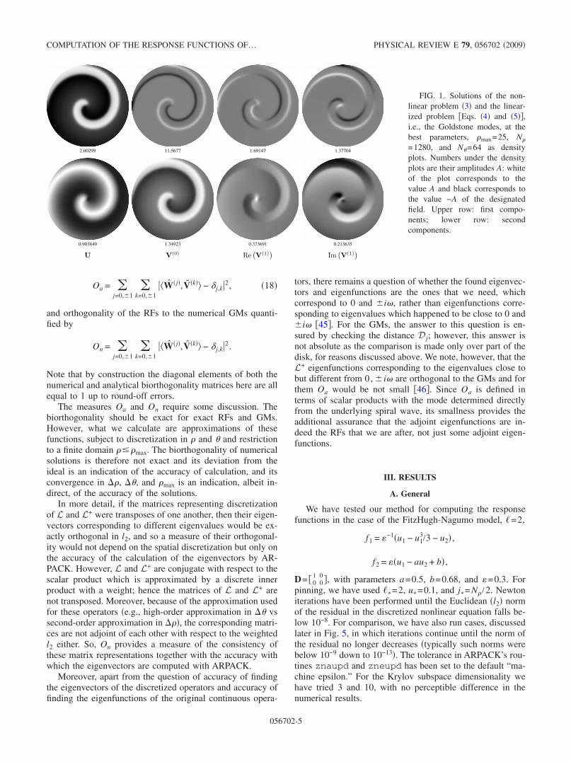
2.00299 11.5677 1.69147 1.37704

0.903849 1.34923 0.373691 0.213635

U V(0) Re(V(1)

)Im

(V(1)

)

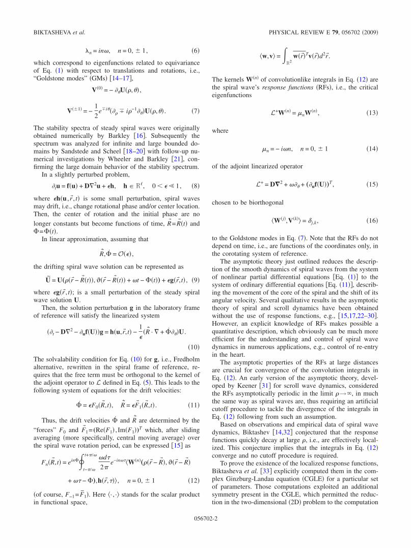
FIG. 1. Solutions of the non-linear problem �3� and the linear-ized problem �Eqs. �4� and �5��,i.e., the Goldstone modes, at thebest parameters, �max=25, N�

=1280, and N=64 as densityplots. Numbers under the densityplots are their amplitudes A: whiteof the plot corresponds to thevalue A and black corresponds tothe value −A of the designatedfield. Upper row: first compo-nents; lower row: secondcomponents.

COMPUTATION OF THE RESPONSE FUNCTIONS OF… PHYSICAL REVIEW E 79, 056702 �2009�

056702-5

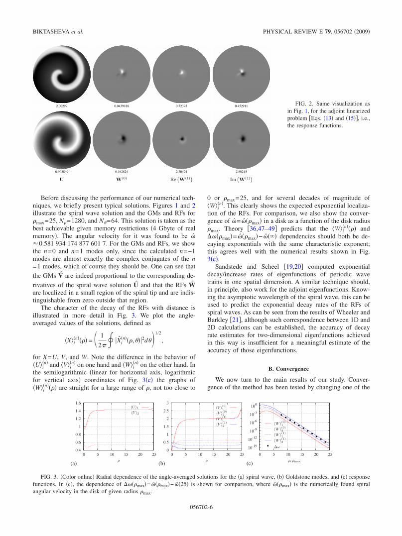
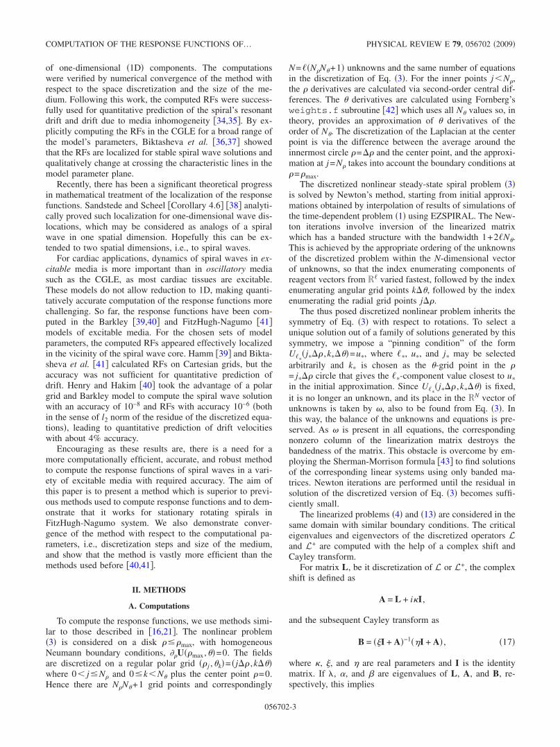
Before discussing the performance of our numerical tech-niques, we briefly present typical solutions. Figures 1 and 2illustrate the spiral wave solution and the GMs and RFs for�max=25, N�=1280, and N=64. This solution is taken as thebest achievable given memory restrictions �4 Gbyte of realmemory�. The angular velocity for it was found to be ��0.581 934 174 877 601 7. For the GMs and RFs, we showthe n=0 and n=1 modes only, since the calculated n=−1modes are almost exactly the complex conjugates of the n=1 modes, which of course they should be. One can see that

the GMs V are indeed proportional to the corresponding de-

rivatives of the spiral wave solution U and that the RFs Ware localized in a small region of the spiral tip and are indis-tinguishable from zero outside that region.

The character of the decay of the RFs with distance isillustrated in more detail in Fig. 3. We plot the angle-averaged values of the solutions, defined as

�X�i�n���� = 1

2�� Xi

�n���,�2d�1/2

,

for X=U, V, and W. Note the difference in the behavior of�U�i

�n� and �V�i�n� on one hand and �W�i

�n� on the other hand. Inthe semilogarithmic �linear for horizontal axis, logarithmicfor vertical axis� coordinates of Fig. 3�c� the graphs of�W�i

�n���� are straight for a large range of �, not too close to

0 or �max=25, and for several decades of magnitude of�W�i

�n�. This clearly shows the expected exponential localiza-tion of the RFs. For comparison, we also show the conver-gence of �= ���max� in a disk as a function of the disk radius�max. Theory �36,47–49� predicts that the �W�i

�n���� and����max�= ���max�− ���� dependencies should both be de-caying exponentials with the same characteristic exponent;this agrees well with the numerical results shown in Fig.3�c�.

Sandstede and Scheel �19,20� computed exponentialdecay/increase rates of eigenfunctions of periodic wavetrains in one spatial dimension. A similar technique should,in principle, also work for the adjoint eigenfunctions. Know-ing the asymptotic wavelength of the spiral wave, this can beused to predict the exponential decay rates of the RFs ofspiral waves. As can be seen from the results of Wheeler andBarkley �21�, although such correspondence between 1D and2D calculations can be established, the accuracy of decayrate estimates for two-dimensional eigenfunctions achievedin this way is insufficient for a meaningful estimate of theaccuracy of those eigenfunctions.

B. Convergence

We now turn to the main results of our study. Conver-gence of the method has been tested by changing one of the

2.00299 0.0439188 0.72395 0.452911

0.903849 0.162824 2.70424 2.80215

U W(0) Re(W(1)

)Im

(W(1)

)

FIG. 2. Same visualization asin Fig. 1, for the adjoint linearizedproblem �Eqs. �13� and �15��, i.e.,the response functions.

0.4

0.6

0.8

1

1.2

1.4

1.6

0 5 10 15 20 25

�U�1�U�2

ρ

0

0.5

1

1.5

2

2.5

3

0 5 10 15 20 25

�V �(0)1

�V �(0)2

�V �(1)1

�V �(1)2

ρ

10-15

10-12

10-9

10-6

10-3

100

0 5 10 15 20 25

�W �(0)1

�W �(0)2

�W �(1)1

�W �(1)2

∆ω

ρ, ρmax(a) (b) (c)

FIG. 3. �Color online� Radial dependence of the angle-averaged solutions for the �a� spiral wave, �b� Goldstone modes, and �c� responsefunctions. In �c�, the dependence of ����max�= ���max�− ��25� is shown for comparison, where ���max� is the numerically found spiralangular velocity in the disk of given radius �max.

BIKTASHEVA et al. PHYSICAL REVIEW E 79, 056702 �2009�

056702-6

three numerical approximation parameters �max, N�, and N

while keeping the other two at the fixed values set by the“best example.” More specifically, while changing �max, weconsider two variants: one with fixed N, and one withchanging N so that the combination �max�, which is thesize of the outermost computational cells in the angular di-rection, remains constant.

Figure 4 illustrates the results of the study, where the fourcolumns correspond to different series of calculations, andthe three rows correspond to the three different methods ofassessing the accuracy: closeness of the eigenvalues to thetheoretical values, distance between numerical and analyticalGMs, and orthogonality between nondual RFs and GMs. Thescales of ��, �, and the error estimates are logarithmic, andthe scales of �max are linear. Shown here is the distance be-tween the numerical and analytical Goldstone modes in L2norm, the distance in C0 norm looks similar.

A typical feature on many of the curves is a “knee” shapewhen the measure of the error decreases as �max grows or �or �� decrease, but only until a certain point, beyond whichit reaches a plateau. This behavior is expected and expli-cable. The calculation error is affected by many factors, andif the factor varied in a particular series becomes negligible,

then the error remains at a constant level determined by fixedvalues of other factors.

The position of the knees on the curves indicates that theaccuracy of the rotational �n=0� modes would be improvedif � were further decreased �there are no knees on thecurves corresponding to the rotational modes, red online, inthe fourth, i.e., rightmost column�, whereas the limiting pa-rameter for the translational �n=1� modes is �� �there are noknees on the curves corresponding to the translationalmodes, blue online, in the third column�. The analysis of thefirst two columns is more complicated. The error estimates atthe maximal �max are similar in both columns as they corre-spond to the same best spiral. These limit values areachieved, i.e., plateaus are observed, at much smaller �maxvalues if �=const, than if �max�=const. This is becausereduction in �max at fixed � produces an additional im-provement of approximation due to the angular discretiza-tion. When �max� is kept fixed, as in the first column, thedependence of the solution on the disk radius is without thisextra benefit.

The rates of convergence with respect to parameters canbe assessed by the slopes of the curves above the knees be-fore they plateau. In some cases the data are somewhat ir-

eige

nval

ues

10-16

10-14

10-12

10-10

10-8

10-6

10-4

10-2

100

|λ1 − iω||λ0|

|µ1 + iω||µ0|

∆ω

|λ1 − iω||λ0|

|µ1 + iω||µ0|

∆ω

|λ1 − iω||λ0|

|µ1 + iω||µ0|

∆ω

|λ1 − iω||λ0|

|µ1 + iω||µ0|

∆ω

(a) (b) (c) (d)

dist

ance

10-14

10-12

10-10

10-8

10-6

10-4

10-2D1D0 D1

D0 D1D0 D1

D0

(e) (f) (g) (h)

orth

ogon

ality

10-9

10-8

10-7

10-6

10-5

10-4

10-3

10-2

10-1

8 10 12 14 16 18 20 22 24 26

OnOa

ρmax (ρmax∆θ = const)

8 10 12 14 16 18 20 22 24 26

OnOa

ρmax (∆θ = const)

10-2 10-1 100

OnOa

∆ρ

0.1 0.2 0.3

OnOa

∆θ(i) (j) (k) (l)

FIG. 4. �Color online� Convergence in numerical parameters of deviation of the numerical eigenvalues from theoretical �upper row�, ofL2 distance between numerical and theoretical eigenfunctions �second row�, and of orthogonality, i.e., Frobenius norm of the difference ofthe matrix of scalar products of eigenfunctions and adjoint eigenfunctions from the unity matrix �third row�, all in logarithmic scales, asdependencies of disk radius �first and second columns, linear scale�, radius discretization step �third column, logarithmic scale�, and polarangle discretization step �fourth column, logarithmic scale�. In the first column, �max is changed while the values of �� and �max� are keptconstant. In the second column, �max is changed while �� and � are kept constant.

COMPUTATION OF THE RESPONSE FUNCTIONS OF… PHYSICAL REVIEW E 79, 056702 �2009�

056702-7

regular, primarily at parameters corresponding to lower val-ues of error estimates. This is not unexpected and weattribute it to the incomplete convergence of the iterativeprocedures �see below�. On the whole, the slopes can bedetermined clearly from these plots.

The constant slope in the first �leftmost� and the secondcolumns corresponds to the exponential convergence with�max. The constant slope in the third column corresponds topower-law convergence, and the typical slope is 2. This iswell seen on the curves for translational modes, blue online,and not well on the curves for rotational modes, red online,which are very small anyway. Slope 2 in the third column isto be expected as our discretization is second order in �� inall cases. The curves in the fourth �rightmost� column areconvex, which is consistent with the fact that the order ofapproximation is N, which varies along the curve as �varies, since N=2� /�, so the slope is bigger for smaller�. In other words, the high order of the Fornberg approxi-mation of the derivatives implies that the convergence in� is faster than any fixed power.

The irregular shape of some of the curves in Fig. 4 at verylow values of the error estimates is related to the accuracy offinding the spiral solution and is ultimately affected by theprecision of floating-point computations. Note that all calcu-lations in Fig. 4 have been performed with a tolerance of10−8 for Newton iterations of the spiral wave and some of thecurves fall as low as 10−15, i.e., close to machine epsilon. Achange in the tolerance of the Newton iteration reduces ir-regularities in the curves at low values, as shown in Figs.5�a� and 5�b�.

Finally, Fig. 5�c� illustrates the convergence of numerical

RFs W�0,1� as ��→0, calculated as the L2-distance E0,1 be-tween the solutions at a given resolution �� and the bestsolution calculated at the smallest ���=25 /1280. As ex-plained in the Sec. II B, this comparison has been restrictedto the series of calculations with varying ��, where grids atlower resolutions were subgrids of those with higher resolu-tions. The graphs of C0 distances E0,1� looked similar and arenot shown here.

IV. DISCUSSION

The main result of this paper is a general robust methodfor obtaining response functions for rigidly rotating spiral

waves in excitable media with required accuracy. We havetested the method on the FitzHugh-Nagumo model, and wehave studied the convergence of spiral wave solutions andeigenfunctions, both the Goldstone modes and the responsefunctions, with respect to the numerical approximation pa-rameters �max, N�, and N. The rates of convergence arefound to agree with the order of approximation and indicatethe accuracy with which solutions can be found for particularnumerical parameters.

The slowest �second-order� convergence is, as expected,in the parameter N�. Thus in a typical situation, an improve-ment of accuracy requires, other things being equal, an in-crease in N�, with associated increase in memory and timedemands. Thus, the most promising avenue of further devel-opment of the method is via an increase in the approximationorder of the radial derivatives. This is, of course, subject tousual caveat that the degree of approximation should be con-sistent with the actual smoothness of the solutions.

The method used here to solve the eigenvalue problemsfor operators L relies on successive application of transfor-mations of L applied to a sequence of vectors, alternatingwith the Gram-Schmidt orthogonalization. These are typicalideas, also used in �40,41�. The difference is that in �40,41�,the linear transformations were polynomial functions of Lwhereas we use rational functions of L. The polynomial it-erations used in �40,41� were in fact equivalent to solving aCauchy problem for equation du /dt=Lu by the explicit Eu-ler method. Therefore, those methods require a large numberof iterations, and convergence speed of the iterations de-pends on the smallness of the absolute difference of the realparts of the eigenvalues of interest compared to those ofother eigenvalues. One requires at least O�105� and typicallyO�106� sparse matrix-vector multiplications to achieve thedesired solutions to the eigenvalue problem using such anapproach.

In contrast, with the complex shift and inversion of Lused in this paper, the convergence speed of the iterationsdepends on the smallness of the distance of the eigenvaluesfrom their theoretical values used in the complex shift, com-pared to the distance to other eigenvalues. Hence the numberof iterations required is very small, typically O�10�. Morespecifically, with Krylov subspace dimensionality 3, thenumber of matrix multiplications with matrix B of Eq. �17�did not exceed 7 per one eigenpair; with Krylov subspacedimensionality 10, this number rose to 10. The price to pay

eige

nval

ues

10-16

10-14

10-12

10-10

10-8

10-6

10-4

10-2

100

10-2 10-1 100

|λ1 − iω||λ0|

|µ1 + iω||µ0|

∆ω

10-2 10-1 100

|λ1 − iω||λ0|

|µ1 + iω||µ0|

∆ω

RF

erro

r

10-4

10-3

10-2

10-1

100

101

10-2 10-1 100

E0E1

(a) ∆ρ (b) ∆ρ (c) ∆ρ

FIG. 5. �Color online� ��a� and �b�� Effect of the accuracy of the unperturbed spiral wave solution on the convergence: �a� Newton-iteration tolerance 10−8 and �b� Newton iterations until the norm of the residual stopped decreasing. �c� Convergence of the responsefunctions in ��.

BIKTASHEVA et al. PHYSICAL REVIEW E 79, 056702 �2009�

056702-8

for this acceleration is the necessity to solve large systems oflinear equations. However, the key observation is that sincethe linear system is fixed, it needs to be factorized only once,for a given complex shift, and used for all iterations. Multi-plication by matrix B is achieved with only inexpensiveback/forward solves. Moreover, due to the way we orderedthe unknowns in the discretized problem, the sparcity of ma-trix B does not depend on the order of approximation of derivatives. Hence, we are able to employ high-order ap-proximations requiring far fewer points in the direction forthe same accuracy as the second-order finite difference dis-cretization used in �40�, thereby further improving the effi-ciency of our method.

Discounting the factorization step, each iteration, whichinvolves multiplication by B, is comparable to multiplica-tions by L. In practice we find that the factorization itselfdoes not require more than the equivalent of four to six ac-tions of B. On a MacPro with 3 GHz Intel processor, thefactorization step takes, e.g., about 7.5 s for the grid N�

=1280, N=64, and 0.67 s for the grid N�=640, N=32; thecomputation times per B multiplication were 1.23 and 0.17 s,respectively.

The comparison of our present method with �41� is un-equivocal: matrix inverses were not used there, and it wasadmitted already in �41� that the resulting accuracy of solu-tions was severely limited. While direct accuracy and timingcomparisons with �40� would be most convincing, that codeis not publicly available. However, for reasons already noted,on any given polar grid, the method we report is more accu-

rate due to the angular discretization and considerably fasterin floating-point operations.

The computed response functions are localized in the vi-cinity of the spiral wave tip and exponentially decay withdistance from it. This localization ensures convergence of theconvolution integral in Eq. �12� in an unbounded domain.The eigenvectors of the linearized operator, i.e., Goldstonemodes and of its adjoint, i.e., the response functions havebeen computed using the same technique, so the qualitativelydifferent behavior of these solutions at large � is not a nu-merical artifact, as it was not in any way assumed in thenumerical method.

Although the method has been used here to compute theresponse functions in the FitzHugh-Nagumo model, none ofthe details of the method depends on any specifics of theparticular reaction kinetics and should be widely applicableto the computation of response functions of rigidly rotatingwaves in any other model of excitable tissue, as long as itsright-hand sides are continuously differentiable so the linear-ized theory is applicable. Moreover, the method can also beextended in a straightforward way to include additional ef-fects, such as the effect of uniform twist along scroll waveswith linear filaments in three dimensions �17,40,50�.

ACKNOWLEDGMENT

This study was supported in part by EPSRC under GrantNos. EP/D074789/1 and EP/D074746/1.

�1� T. Frisch, S. Rica, P. Coullet, and J. M. Gilli, Phys. Rev. Lett.72, 1471 �1994�.

�2� D. J. Yu, W. P. Lu, and R. G. Harrison, J. Opt. B: QuantumSemiclassical Opt. 1, 25 �1999�.

�3� B. F. Madore and W. L. Freedman, Am. Sci. 75, 252 �1987�.�4� L. S. Schulman and P. E. Seiden, Science 233, 425 �1986�.�5� A. M. Zhabotinsky and A. N. Zaikin, in Oscillatory Processes

in Biological and Chemical Systems, edited by E. E. Selkov,A. A. Zhabotinsky, and S. E. Shnol �Nauka, Moscow, 1971�, p.279, in Russian.

�6� S. Jakubith, H. H. Rotermund, W. Engel, A. von Oertzen, andG. Ertl, Phys. Rev. Lett. 65, 3013 �1990�.

�7� K. Agladze and O. Steinbock, J. Phys. Chem. A 104, 9816�2000�.

�8� M. A. Allessie, F. I. M. Bonk, and F. Schopman, Circ. Res. 33,54 �1973�.

�9� N. A. Gorelova and J. Bures, J. Neurobiol. 14, 353 �1983�.�10� F. Alcantara and M. Monk, J. Gen. Microbiol. 85, 321 �1974�.�11� J. Lechleiter, S. Girard, E. Peralta, and D. Clapham, Science

252, 123 �1991�.�12� A. B. Carey, R. H. Giles, Jr., and R. G. Mclean, Am. J. Trop.

Med. Hyg. 27, 573 �1978�.�13� J. D. Murray, E. A. Stanley, and D. L. Brown, Proc. R. Soc.

London, Ser. B 229, 111 �1986�.�14� V. N. Biktashev, Ph.D. thesis, Moscow Institute of Physics and

Technology, 1989.

�15� V. Biktashev and A. Holden, Chaos, Solitons Fractals 5, 575�1995�.

�16� D. Barkley, Phys. Rev. Lett. 68, 2090 �1992�.�17� V. N. Biktashev, Physica D 36, 167 �1989�.�18� B. Sandstede and A. Scheel, Physica D 145, 233 �2000�.�19� B. Sandstede and A. Scheel, Phys. Rev. E 62, 7708 �2000�.�20� B. Sandstede and A. Scheel, Phys. Rev. Lett. 86, 171 �2001�.�21� P. Wheeler and D. Barkley, SIAM J. Appl. Dyn. Syst. 5, 157

�2006�.�22� V. A. Davydov, V. S. Zykov, A. S. Mikhailov, and P. K. Brazh-

nik, Izv. Vyssh. Uchebn. Zaved., Radiofiz. 31, 574 �1988�.�23� V. S. Zykov, Biofizika 32, 337 �1987�.�24� J. P. Keener and J. J. Tyson, Physica D 44, 191 �1990�.�25� J. P. Keener and J. J. Tyson, Physica D 53, 151 �1991�.�26� V. A. Davydov, V. S. Zykov, and A. S. Mikhailov, Usp. Fiz.

Nauk 161, 45 �1991�.�27� V. N. Biktashev and A. V. Holden, J. Theor. Biol. 169, 101

�1994�.�28� V. N. Biktashev, Int. J. Bifurcation Chaos Appl. Sci. Eng. 8,

677 �1998�.�29� V. Krinsky, E. Hamm, and V. Voignier, Phys. Rev. Lett. 76,

3854 �1996�.�30� H. Henry, Phys. Rev. E 70, 026204 �2004�.�31� J. Keener, Physica D 31, 269 �1988�.�32� V. N. Biktashev, A. V. Holden, and H. Zhang, Philos. Trans. R.

Soc. London, Ser. A 347, 611 �1994�.

COMPUTATION OF THE RESPONSE FUNCTIONS OF… PHYSICAL REVIEW E 79, 056702 �2009�

056702-9

�33� I. V. Biktasheva, Y. E. Elkin, and V. N. Biktashev, Phys. Rev.E 57, 2656 �1998�.

�34� I. V. Biktasheva, Y. E. Elkin, and V. N. Biktashev, J. Biol.Phys. 25, 115 �1999�.

�35� I. V. Biktasheva, Phys. Rev. E 62, 8800 �2000�.�36� I. V. Biktasheva and V. N. Biktashev, J. Nonlinear Math. Phys.

8, 28 �2001�.�37� I. V. Biktasheva and V. N. Biktashev, Phys. Rev. E 67, 026221

�2003�.�38� B. Sandstede and A. Scheel, SIAM J. Appl. Dyn. Syst. 3, 1

�2004�.�39� E. Hamm, Ph.D. thesis, Institut Non Linéair de Nice, Univer-

sité de Nice–Sophia Antipolice, 1997.�40� H. Henry and V. Hakim, Phys. Rev. E 65, 046235 �2002�.�41� I. V. Biktasheva, A. V. Holden, and V. N. Biktashev, Int. J.

Bio-Med. Comput. 16, 1547 �2006�.�42� B. Fornberg, A Practical Guide to Pseudospectral Methods

�Cambridge University Press, Cambridge, UK, 1998�.�43� W. Press, B. Flannery, S. Teukolsky, and W. Vetterling,

Numerical Recipes in C �Cambridge University Press, Cam-bridge, UK, 1992�.

�44� R. B. Lehoucq, D. C. Sorensen, and C. Yang, ARPACK Users’Guide �SIAM, Philadelphia, 1998�.

�45� Close neighbors of the translational eigenmodes are always apossibility in a large enough disk, see �21�.

�46� Equation �18� gives Oa=3 if all nine scalar products vanish;however in reality the scalar products of respective GMs andRFs are used for normalization, so in the case of wrong RFs,all scalar products would be divided by small numbers whichmay result in rather large values of Oa.

�47� P. S. Hagan, SIAM J. Appl. Math. 42, 762 �1982�.�48� V. N. Biktashev, in Nonlinear Waves II: Dynamics and Evolu-

tion, edited by A. V. Gaponov-Grekhov, M. I. Rabinovich, andJ. Engelbrecht �Springer, Berlin, 1989�, pp. 87–96.

�49� B. Sandstede �personal communication�.�50� D. Margerit and D. Barkley, Phys. Rev. Lett. 86, 175

�2001�.

BIKTASHEVA et al. PHYSICAL REVIEW E 79, 056702 �2009�

056702-10