Computation of the homotopy of the spectrum tmftilmanb/papers/computation... · Computation of the homotopy of the spectrum tmf 13 Deﬁnition The category of Hopf algebroids over

Geometry & Topology Monographs 13 (2008) 11–40 11

Computation of the homotopy of the spectrum tmf

TILMAN BAUER

This paper contains a complete computation of the homotopy ring of the spectrumof topological modular forms constructed by Hopkins and Miller. The computationis done away from 6 , and at the (interesting) primes 2 and 3 separately, and ineach of the latter two cases, a sequence of algebraic Bockstein spectral sequences isused to compute the E2 term of the elliptic Adams–Novikov spectral sequence fromthe elliptic curve Hopf algebroid. In a further step, all the differentials in the latterspectral sequence are determined. The result of this computation is originally due toHopkins and Mahowald (unpublished).

55N34; 55T15

1 Introduction

In [2; 3; 4], Hopkins, Mahowald, and Miller constructed a new homology theorycalled tmf, or topological modular forms (it was previously also called eo2 ). Thistheory stands at the end of a development of several theories called elliptic cohomology(Landweber, Ravenel and Stong [9] Landweber [8], Franke[1] and others). The commonwish was to produce a universal elliptic cohomology theory, ie, a theory Ell togetherwith an elliptic curve Cu over �0 Ell such that for any complex oriented spectrum E

and any isomorphism of the formal group associated to E with the formal completionof a given elliptic curve C , there are unique compatible maps Ell!E and Cu! C .It was immediately realized that this is impossible due to the nontriviality of theautomorphisms of the “universal” elliptic curve. Earlier theories remedied this byinverting some small primes (eg, by considering this moduli problem over ZŒ1=6�),or by considering elliptic curves with level structures, or both. The Hopkins–Millerapproach, however, is geared in particular towards studying the small prime phenomenathat arise; as a trade-off, their theory tmf is not complex orientable. This, however,turned out to have positive aspects. Hopkins and Mahowald first computed the homotopygroups of tmf and realized that the Hurewicz map ��S0!��tmf detects surprisinglymany classes, at least at the primes 2 and 3; thus tmf was found to be a rather goodapproximation to the stable stems themselves at these primes. Their computation wasnever published, and the aim of this note is to give a complete calculation (in a differentway than theirs) of the homotopy of tmf at the primes 2 and 3.

Published: 22 February 2008 DOI: 10.2140/gtm.2008.13.11

12 Tilman Bauer

Along with the construction of tmf, which is constructed as an A1–ring spectrumand is shown to be E1 , Hopkins and Miller set up an Adams–Novikov type spectralsequence that converges to ��.tmf/; its E2 term is given as an Ext ring of a Hopfalgebroid,

Es;t2D Exts;t

.A;�/.A;A/;

where all the structure of the Hopf algebroid .A; �/ can be described completelyexplicitly. One particular feature of this Hopf algebroid is that both A and � arepolynomial rings over Z on finitely many generators; it is this finiteness that generatesa kind of periodicity in ��.tmf/ and makes it possible to compute the whole ring andnot only the homotopy groups up to a certain dimension.

In Section 2 I will review some notions and tools from the homological algebra ofHopf algebroids; in Section 3, the elliptic curve Hopf algebroid is defined and studied.The short Section 4 contains the computation of ��tmf away from 6; Sections 5 and6 contain the computation of the Ext term and the differentials, respectively, of thespectral sequence at the prime 3; in Sections 7 and 8, the same is done for the prime 2.

Acknowledgements I do not claim originality of any of the results of this paper. Asalready noted, the computation was first done by Hopkins and Mahowald. Rezk [11]also has some lecture notes with an outline of the computations that need to be donewhen computing the homotopy from the Hopf algebroid. I found it worthwhile to makethis computation available anyway since it is, in my opinion, an interesting computation,and explicit knowledge of it is useful when using tmf as an approximation to stablehomotopy theory.

I am very grateful to Doug Ravenel, Andy Baker, John Rognes, and the anonymousreferee for suggesting a number of improvements and corrections of this computation.Most importantly, I am deeply indepted to Mike Hopkins, my thesis advisor, from whoI learned everything I know today about tmf.

The LATEX package sseq which produced the numerous spectral sequence charts inthis paper, is available from CTAN servers or from the author’s home page.

2 Homological algebra of Hopf algebroids

In this section I review some important constructions that help in computing thecohomology of Hopf algebroids. All of this is well-known to the experts, but explicitreferences are a little hard to come by.

Geometry & Topology Monographs, Volume 13 (2008)

Computation of the homotopy of the spectrum tmf 13

Definition The category of Hopf algebroids over a ring k is the category of co-groupoid objects .A; �/ in the category of commutative k –algebras such that the left(equivalently, right) unit map �LW A! � (resp. �R ) is flat.

The category of left comodules over a Hopf algebroid .A; �/ is the category of .A; �/–left coaction objects in k –modules.

(For a more explicit description, consult Ravenel [10, Appendix A1].)

By convention, we will always consider � as an A–module using the left unit �L

unless otherwise stated. The flatness condition (which not all authors consider part ofthe definition of a Hopf algebroid) ensures that the category of comodules is an abeliancategory, which has enough injectives so that homological algebra is possible. We willabbreviate

H n.A; �IM /D Extn.A;�/�comod.A;M /:

and H�.A; �/ D H�.A; �IA/. In our situation, all objects are Z-graded, and wewrite

H n;m.A; �IM /D Extn.A;�/�comod.A;M Œ�m�/

where .M Œm�/n DMn�m .

Definition A natural transformation between two maps of Hopf algebroids

f D .f0; f1/; g D .g0;g1/W .A; �/! .A0; � 0/

is a natural transformation of functors between cogroupoid objects; explicitly, it is analgebra map cW � ! A0 such that c ı �L D f0 and c ı �R D g0 , and such that thefollowing two composites are equal:

A0˝A �**VVVVV

� // �˝A �

c˝id 33ggggg

id˝c++WWWWW � 0;

�˝A A0

44iiiiii

where is the Hopf algebroid diagonal. In the lower row, A0 is an A–module bymeans of the map f0 , and the rightmost map is induced by f�W �˝A A0! � 0˝A0 A0 .The upper row is defined analogously with g .

An equivalence of Hopf algebroids .A; �/' .A0; � 0/ consists of maps

f W .A; �/� .A0; � 0/ Wgand natural transformations between the identity and f ıg and between the identityand g ıf .


14 Tilman Bauer

2.1 Remark The condition that c ı �L D id for a natural transformation from theidentity to f ıg is saying that c is an A–algebra map.

An equivalence of Hopf algebroids induces an equivalence of comodule categories; inparticular,

H�.A; �IM /ŠH�.A0; � 0If�M /:

2.2 Remark In the language of stacks, this has the following interpretation. Toevery Hopf algebroid .A; �/ there is associated a stack M.A;�/ ; this assignment isleft adjoint to the inclusion of stacks into groupoid valued functors. Equivalent Hopfalgebroids give rise to equivalent associated stacks. The Hopf algebroid cohomologywith coefficients in the comodule M can be interpreted as the cohomology of thequasi-coherent sheaf zM on the stack.

2.3 Base change

Let .A; �/ be any Hopf algebroid, and let A! A0 be a morphism of rings. Define� 0 DA0˝A �˝A A0 , where the left tensor product is built using the map �LW A! � ,and the right one using �RW A! � . Then .A0; � 0/ is also a Hopf algebroid, and thereis a canonical map of Hopf algebroids .A; �/! .A0; � 0/.

The following theorem is proved by Hovey and Sadofsky [6, Theorem 3.3] and Hovey[5, Corollary 5.6]. The authors attribute it to Hopkins.

2.4 Theorem If .A; �/! .A0; � 0/ is such a map of Hopf algebroids, and there existsa ring R and a morphism A0˝A �!R such that the composite

A1˝�R��!A0˝A �!R

is faithfully flat, then it induces an equivalence of comodule categories, and in particularan isomorphism

H�.A; �/Š�!H�.A0; � 0/

This theorem is reminiscent of the change of rings theorem [10, A1.3.12]. In fact, thechange of rings theorem is enough to prove all the consequences of the above theoremused in this work, but I will use Theorem 2.4 for expository reasons.



2.5 The algebraic Bockstein spectral sequence

Let I G .A; �/ be an invariant ideal of a Hopf algebroid, ie, I GA and �R.I/� I� .Denote by .A; �/=I the induced Hopf algebroid .A=I; In�=I/.2.6 Theorem (Miller, Novikov) There is a spectral sequence of algebras, called thealgebraic Bockstein spectral sequence or the algebraic Novikov spectral sequence:

E2 DH��.A; �/ =I I In=InC1

�H)H�.A; �/

arising from the filtration of Hopf algebroids induced by the filtration

0<A=I <A=I2 < � � �<A

If A is Cohen–Macaulay and I GA is a regular ideal, then In=InC1 Š Symn.I=I2/.

In the applications in this paper, I D .x/ will always be a principal ideal, andSym�.I=I2/ D A0Œy� will be a polynomial algebra. Thus the E2 term simplifiesto

E2 DH� ..A; �/ =I/ Œy�:

If x D p , then this is the ordinary (bigraded) Bockstein spectral sequence. In thetopological context, Hopf algebroids are usually graded, and thus the spectral sequenceis really tri-graded. In displaying charts, I will disregard the homological filtrationdegree in the above spectral sequence.

3 The elliptic curve Hopf algebroid

The Hopf algebroid of Weierstrass elliptic curves and their (strict) isomorphisms isgiven by:

AD ZŒa1; a2; a3; a4; a6�I jai j D 2i I� DAŒr; s; t �I jr j D 4I jsj D 2I jt j D 6

and the following structure maps:

The left units �L are given by the standard inclusion A ,! � , the right units are:

�R.a1/D a1C 2s

�R.a2/D a2� a1sC 3r � s2

�R.a3/D a3C a1r C 2t

�R.a4/D a4� a3sC 2a2r � a1t � a1rs� 2st C 3r2

�R.a6/D a6C a4r � a3t C a2r2� a1r t � t2C r3:


16 Tilman Bauer

The comultiplication map is given by:

.s/D s˝ 1C 1˝ s

.r/D r ˝ 1C 1˝ r

.t/D t ˝ 1C 1˝ t C s˝ r:

This Hopf algebroid classifies plane cubic curves in Weierstrass form; the universalWeierstrass curve is defined over A in affine coordinates .x;y/ as

(3.1) y2C a1xyC a3y D x3C a2x2C a4xC a6;

and the universal strict isomorphism classified by � is the coordinate change

x 7! xC r

y 7! yC sxC t:

It is easy, and classical, to compute the ring of invariants of this Hopf algebroid:

H 0;�.A; �/D ZŒc4; c6; ��=.c34 � c2

6 � 1728�/

where the classes c4 , c6 , � are given in the universal case, and hence for everyWeierstrass curve, by the equations (cf Silverman [12, III.1])

b2 D a21C 4a2

b4 D 2a4C a1a3

b6 D a23C 4a6

c4 D b22 � 24b4

c6 D�b32 C 36b2b4� 216b6

�D 11728

.c34 � c2

6/:

A cubic of the form (3.1) is an elliptic curve if and only if �, the discriminant, isinvertible. An elliptic curve is a 1–dimensional abelian group scheme, and thus thecompletion at the unit (which is the point at infinity) is a formal group. In fact, thisconstruction even gives a formal group when the discriminant is not invertible becausethe point at infinity in a Weierstrass curve is always a smooth point. Thus we get a mapof Hopf algebroids

H W .M U�;M U�M U /! .A; �/:

and a map from the M U –based Adams–Novikov spectral sequence to the ellipticspectral sequence, which converges to the Hurewicz map hW S0 ! tmf. This laststatement is due to the fact that there is a complex oriented ring spectrum A with



��ADA; it can be constructed as AD tmf^Y .4/, where Y .4/ is the Thom spectrumof �U.4/! Z�BU (Rezk [11, Sections 12–14]).

Let M U�DZŒx1;x2; : : : � with jxi j D 2i , and M U�M U DM U�Œm1;m2; : : : � withjmi j D 2i . By direct verification, we may choose the generators xi ; mi such that

(3.2) H.xi/D ai for i D 1; 2IH.m1/D s and H.m2/D r:

This very low-dimensional observation enables us to compare the tmf spectral se-quence with the usual M U –Adams–Novikov spectral sequence and will be the key todetermining the differentials in sections 6 and 8.

4 The homotopy of tmf at primes p > 3

As was mentioned in the introduction, tmf becomes complex oriented at large primes,and thus the homotopy ring becomes very simple; it is isomorphic to the ring of classicalmodular forms, which is generated by the Eisenstein forms E4 and E6 .

We first state a result valid whenever 2 is invertible in the ground ring.

Let zA D ZŒ 12; a2; a4; a6�, f W AŒ 12 �! zA be the obvious projection map sending a1

and a3 to 0, and

z� D zA˝A �˝AzADAŒ 1

2; r; s; t �=.a1; a3; �R.a1/; �R.a3//D zAŒr �:

4.1 Lemma The Hopf algebroids .AŒ 12�; �Œ 1

2�/ and . zA; z�/ are equivalent.

Proof Define a map gW . zA; z�/! .AŒ12�; �Œ1

2�/ in the opposite direction of f by

g.a2/D a2C 14a2

1;

g.a4/D a4C 12a1a3;

g.a6/D a6C 14a2

3; and

g.r/D r:

Then clearly f ıg D id. zA;z�/

, and if we define cW �Œ 12�!AŒ 1

2� to be A–linear and

c.r/D 0I c.s/D� 12

a1I c.t/D� 12

a3;

we find that c ı �R D g ıf .


18 Tilman Bauer

4.2 Remark This proof is the formal version of the following algebraic argument:As 2 becomes invertible, we can complete the squares in the Weierstrass equation (3.1)by the substitution

y 7! y � 12

a1x� 12

a3:

That is, we can find new parameters x and y such that the elliptic curve is given by

(4.3) y2 D x3C a2x2C a4xC a6:

All the strict isomorphisms of such curves are given by substitutions x 7! xC r , hencethe Hopf algebroid is equivalent to . zA; z�/.

When 3 is also invertible in the ground ring, we can in a similar fashion complete thecube on the right hand side of (4.3) by sending x 7! x� 1

3a2 and obtain

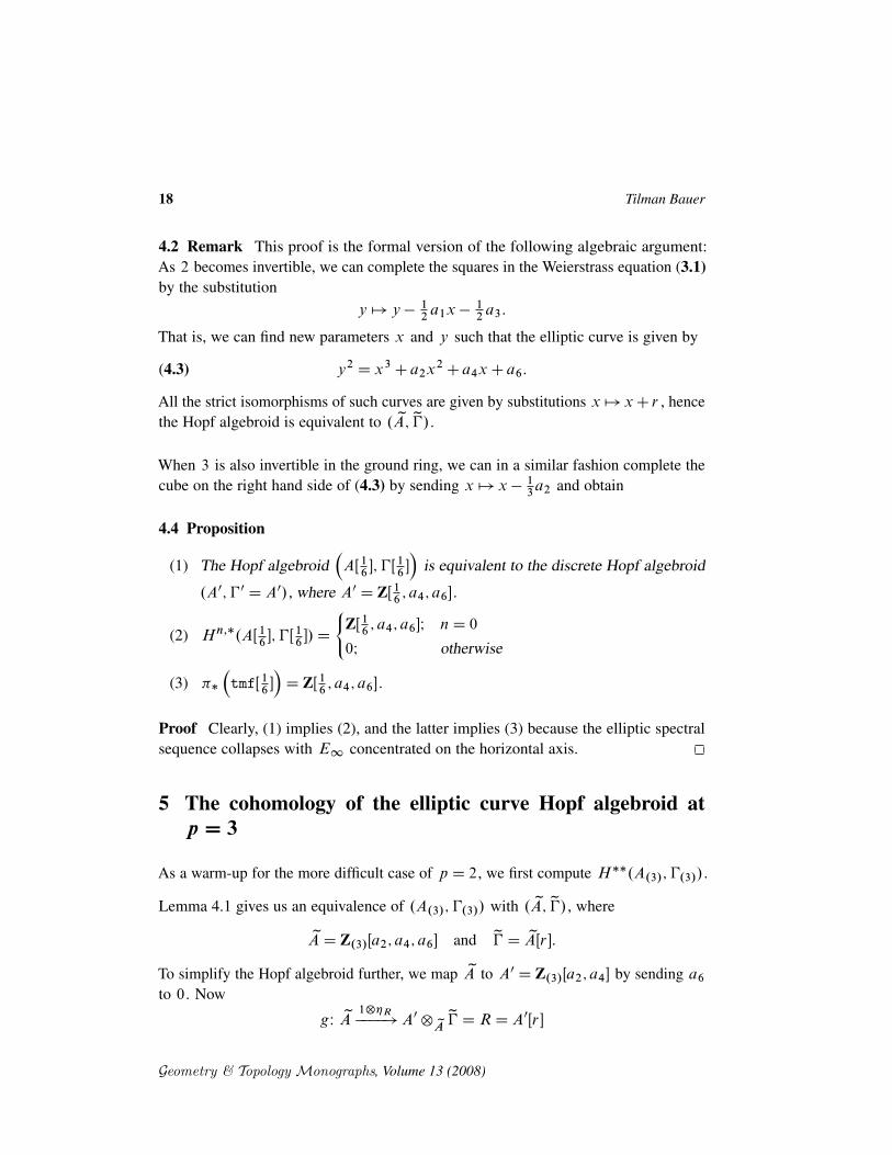
4.4 Proposition

(1) The Hopf algebroid�AŒ1

6�; �Œ1

6��

is equivalent to the discrete Hopf algebroid

.A0; � 0 DA0/, where A0 D ZŒ16; a4; a6�.

(2) H n;�.AŒ16�; �Œ1

6�/D

(ZŒ1

6; a4; a6�I nD 0

0I otherwise

(3) ��

�tmfŒ1

6��D ZŒ1

6; a4; a6�.

Proof Clearly, (1) implies (2), and the latter implies (3) because the elliptic spectralsequence collapses with E1 concentrated on the horizontal axis.

5 The cohomology of the elliptic curve Hopf algebroid atp D 3

As a warm-up for the more difficult case of p D 2, we first compute H��.A.3/; �.3//.

Lemma 4.1 gives us an equivalence of .A.3/; �.3// with . zA; z�/, where

zAD Z.3/Œa2; a4; a6� and z� D zAŒr �:To simplify the Hopf algebroid further, we map zA to A0 D Z.3/Œa2; a4� by sending a6

to 0. Now

gW zA 1˝�R��!A0˝ zA z� DRDA0Œr �



is defined by

g.a2/D a2C 3r

g.a4/D a4C 2a2r C 3r2

g.a6/D a4r C a2r2C r3

This is a faithfully flat extension since g.a6/ is a monic polynomial in r , and weinvoke Theorem 2.4 to conclude that H�.A; �/ŠH�.A0; � 0/ with

.A0; � 0/D�

Z.3/Œa2; a4�;A0Œr �=

�r3C a2r2C a4r

��:

Let I0 D .3/, I1 D .3; a2/, and I2 D .3; a2; a4/ be the invariant prime ideals of.A0; � 0/, and denote by .An; �n/ the Hopf algebroid .A0; � 0/=In for nD 0; 1; 2.

As an A0–module, � 0 is free with basis f1; r; r2g. We first compute the cohomologyof .A2; �2/D .Z=3;Z=3Œr �=.r3//. Since A2 is a field, �2 is injective as an .A2; �2/–comodule, and we can take the minimal resolution

Z=3�L��! �2

@@r��! �2

@2

@r 2��! �2

@@r��! �2

@2

@r 2��! � � �

and get the cohomology algebra

H��.A2; �2/DE.˛/˝P .ˇ/;

where ˛ 2H 1;4.A2; �2/ and ˇ 2H 2;12.A2; �2/.

In the cobar complex, ˛ is represented by Œr � and ˇ by Œr2jr �� Œr jr2�. Furthermore,ˇ can be expressed as a Massey product:

(5.1) ˇ D h˛; ˛; ˛i:

If we consider the algebraic Bockstein spectral sequence associated with the ideal.a4/GA1DZ=3Œa4�DA0=.3; a2/, we see that the polynomial generator correspondingto a4 supports no differentials and hence

H��.A1; �1/DH��.A2; �2/˝P .a4/:


20 Tilman Bauer

We now look at the Bockstein spectral sequence for .a2/GA0DZ=3Œa2; a4�DA0=.3/.We find that in the cobar complex,

a4an2 7! 2anC1

2Œr �

a4Œr �C a2Œr2� 7! 0 Massey product: hanC1

2; ˛; ˛i

a24an

2 7! a4anC12

Œr �

a24Œr �C a4a2Œr

2� 7! a22

�Œr2jr �C Œr jr2�

�D a2

2ˇ

a34 7! 0:

Hence we get the following picture for the E1 term:

0 4 8 12 16 20 240

4

a2

a2ˇ

a2ˇ2

a22

˛

ˇ

ha2; ˛; ˛i

Here, and in all subsequent charts, we use Adams indexing, ie, the square at coordinate.x;y/ represents the group H y;xCy . We also use the following conventions:

� a dot ‘�’ represents a generator of Z=p (here, p D 3);

� a circle around an element denotes a nontrivial Z=p–extension of the grouprepresented by that element;

� a square ‘�’ denotes a generator of Z.p/ ;

� a line of slope 1, 1 or 1=3 denotes multiplication with p , the generator ofH 1;2 (not present at p D 3), or of H 1;4 ;

� an arrow with positive slope denotes generically that the pattern is continued inthat direction;

� an arrow with negative slope denotes a differential; the arrow, the source, and thetarget are then drawn in a gray color to denote that these classes do not survive.

The dashed line of slope 1=3 denotes an exotic multiplicative extensions which followsfrom the Massey product shuffling lemma [10, Appendix 1] and (5.1):

ha2; ˛; ˛i˛ D a2h˛; ˛; ˛i D a2ˇ:



Finally, we run the Bockstein spectral sequence to get the 3–local homology. Thedifferentials derive from d1.a2/D 3r and yield

0 2 4 6 8 10 12 14 16 18 20 22 24 260

2

4

�˛

ˇ

ˇ2

� � � � ��

where � is the discriminant.

6 The differentials

In this section, I compute the differentials in the elliptic spectral sequence whoseE2 –term was computed in the previous section. The differential which implies allfurther differentials in the 3–local tmf spectral sequence is

(6.1) d5.�/D ˇ2˛:

This follows from comparison with the Adams–Novikov spectral sequence: By (3.2),the class Œx2� representing the Hopf map ˛1 2 �3.S0/ in the cobar complex of theAdams–Novikov spectral sequence is mapped to ˛ ; because of the Massey productˇ D h˛; ˛; ˛i, we also conclude that ˇ represents the Hurewicz image of the classˇ1 2 �10.S0/.

Now in the stable stems, ˇ31˛1 represents the trivial homotopy class although ˇ3˛ is

nontrivial in the Hopf algebroid cohomology; thus it must be killed by a differential.The only possibility is ˇ3˛ D d5.�ˇ/, which implies the differential (6.1).

0 4 8 12 16 20 24 28 32 36 400

4

8

� 3

˛ˇ

ˇ2

ˇ3

b

Figure 1: The elliptic spectral sequence at p D 3 up to dimension 40

It also shows that there is an element b representing a class in �27tmf which isthe unique element in the Toda bracket hˇ2

1; ˛1; ˛1i. The Massey product h˛; ˛; ˛i


22 Tilman Bauer

converges to the Toda bracket h˛1; ˛1; ˛1i. The Shuffling Lemma for Toda brackets[10, Appendix 1] implies that there is a multiplicative extension b˛1 D ˇ3

1in �27 as

displayed in the chart. It implies that there has to be a differential d9.�2˛/ D 2ˇ5

since ˇ51D ˇ2

1b˛1 .

The complete E1 term has a free polynomial generator �3 in degree 72 and isdisplayed in Figures 1 and 2, where most classes in filtration 0 have been omitted.

40 44 48 52 56 60 64 68 72 760

4

8

12

16

3 ��3

ˇ4

ˇ5

ˇ6

ˇ7

Figure 2: The elliptic spectral sequence at p D 3 , dimensions 40–76

7 The cohomology of the elliptic curve Hopf algebroid atp D 2

In this section we are going to compute the cohomology of .A; �/, localized at theprime 2.

Note that if 3 is invertible, we can proceed as in Remark 4.2 and complete the cube inx by a transformation x 7! xC r , thereby eliminating the coefficient a2 . This meansthat the resulting Hopf algebroid is

. zA; z�/D .Z.2/Œa1; a3; a4; a6�; zAŒs; t �/;where the map �! z� maps r to 1

3.s2C a1s/.

By two applications of Theorem 2.4, we can furthermore eliminate a4 and a6 (a4

maps to a monic polynomial s4Clower terms in s , a6 to a monic polynomial t2 +lower



terms in t ). This introduces new relations in � :

s4� 6st C a1s3� 3a1t � 3a3s D 0 and

s6� 27t2C 3a1s5� 9a1s2t C 3a21s4� 9a2

1st C a31s3� 27a3t D 0

Hence, at the prime 2, the Hopf algebroid

.A0; � 0/D �Z.2/Œa1; a3�;A0Œs; t �=.the above relations/

�has the same cohomology as .A; �/.

Note that as an A0–module, � 0 is free with basis f1; s; s2; s3; t; st; s2t; s3tg and wehave invariant prime ideals I0 D .2/, I1 D .2; a1/, and I2 D .2; a1; a3/. Define.An; �n/D .A0; � 0/=In for nD 0; 1; 2.

We are going to compute the cohomology of this Hopf algebroid with a sequence ofalgebraic Bockstein spectral sequences. As in the 3–primary case, we first computeH��.A2; �2/. Observe that this is isomorphic as a Hopf algebra to the double DA.1/

of A.1/, where A.1/ is the dual of the subalgebra of the Steenrod algebra generatedby Sq1 and Sq2 .

The cohomology of DA.1/ is well-known. I will compute it here nevertheless todetermine cobar representatives of some classes.

Note that in DA.1/, s2 is primitive, hence we can divide out by it to get a Hopf algebrawhich is isomorphic to the Hopf algebra E.s/˝E.t/. The Cartan–Eilenberg spectralsequence associated to the ideal .s2/ coincides with the algebraic Bockstein spectralsequence of Theorem 2.6 in this situation and has

E1 DH��.DA.1/=.s2//˝P .s2/H)H��.DA.1//:

The cobar complex gives us the following differentials:

d1Œs2nt �D Œs2nC2js�I

d1

�Œt jt �C Œsjs2t �C Œst js2�

�D Œs2js2js2�:

No more differentials are possible for dimension reasons, yielding the following E1–term:

0 2 4 6 8 10 12 14 16 18 20 220

2

4

h1 h2

f

g


24 Tilman Bauer

The elements labeled hi are represented by si ; the element f is represented by

f D Œsjt jt �C Œsjsjs2t �C Œsjst js2C t js2js2�D hh22; h2; h1i;

and the class g is a polynomial generator in this algebra. It is represented in the cobarcomplex by the class Œt jt jt jt � plus elements of higher filtration in the above spectralsequence. It can be expressed as a Massey product

(7.1) g D hh22; h2; h

22; h2i:

as can easily be seen from the differentials.

We record the following Massey product relation:

(7.2) h22 D hh1; h2; h1i

which follows from d Œt �D Œs2js�, d�Œt �C Œs3�

�D Œsjs2�, and

d Œts�D Œt js�C Œsjt C s3�C Œs2js2�:

We will now start an algebraic Bockstein spectral sequence to compute the cohomologyof .A1; �1/ from .A2; �2/:

E1 DH��.DA.1//˝P .a3/H)H��.A1; �1/:

0 2 4 6 8 10 12 14 16 18 20 220

2

4g

h1 h2

a3

f

The elements h1 and h2 lift to cycles in the E1 term, but the cobar complex showsthat

d1.f /D a3h41:

We have an extension a3h31D h3

2because in the cobar complex,

Œt jt �C Œsjs2t �C Œst js2� 7! Œs2js2js2�C a3Œsjsjs�;as well as an exotic Massey product extension

(7.3) a3h21 D hh2; h1; h2i:

Indeed, the Massey product has the cobar representative

Œt js2�C Œs2jt C s3�;



and

d Œs2.t C s3/�D Œt js2�C Œs2jt C s3�C Œs4js�; and s4 D a3s .mod 2; a1/:

No more differentials are possible for dimension reasons.

We thus have computed

E1 D P .a3; h1; h2;g/=.h1h2; h32C a3h3

1/

or, additively only,

E1 D P .a3;g/fh2; h22; h

i1 j i � 0g=.a3h3

1/

It will be necessary to keep track of a Massey product expression for g . Equation (7.1)becomes invalidated because h3

2¤ 0; instead, (7.1) lifts to a matric Massey product

representation

(7.4) g D��

h22

h1

�;

�h2 a3h2

1

a3h21

h2

�;

�h2

2h1

h1 h22

�;

�h2

a3h21

��:

The next step is to introduce a1 . The d1 –differential is linear over P .a23;g/ and

satisfiesd1.a3hi

2/D a1hiC12

where h2 is the lift of the cycle previously called h2 , represented by Œs2C a1s� in thecobar complex.

The resulting homology may be written additively as

P .g/˝ .K˚P .a1/˝L˚H1/

where

K D P .a23/nh2; h

22; h

32

ois the a1 –torsion,

LD P .a23/nhi

1;x;xh1 j 0� i � 3o;

and

H1 D F2

nhi

1 j i � 4o

is the initial infinite h1 –tower. Here

(7.5) x D ha1; h2; h1i


26 Tilman Bauer

is cobar represented by Œa3sC a1t �.

The submodule K˚ 1˝LCH1 constitutes the filtration 0 part; this is displayed inthe following diagram, along with the h1 – and h2 –multiplications:

0 2 4 6 8 10 12 14 16 18 20 22 240

2x

The d2 –differentials all follow from d2.a23/D a2

1x ; explicitly,

d2.a2k3 an

1/D(

a2k�23

anC21

xI k oddI0I k even.

Since d2 does not involve a1 –torsion and is .g; a43/–linear, it is enough to understand

what it does on L=.a43;g/. This module decomposes into two d2 –invariant copies

L0˚ a1L0 of a module L0 , which is shown in the following chart:

0 2 4 6 8 10 12 14 16 18 20 22 240

2

˘ ˘ ˘ ˘ ˘ ˘ ˘a2

1x

a23

da2

1x

Diamonds denote h1 –strings of P .h1/=.h41/ of length 4. Thus

H�.L0; d2/D P .a2

1; h1/=.h41/˚F2 fx;xh1; d; dh1g where d D x2:

The next chart displays the full spectral sequence modulo Bockstein filtration 5 (thefull chart would become too cluttered). Gray classes that do not seem to be hit by or tosupport a differential support a differential into higher filtration.

0 2 4 6 8 10 12 14 16 18 20 22 24 26 28 300

2

4

x a1x

d

y

g

�

The new indecomposable class y has the Massey product representation:

(7.6) y D hx; a21; h2i D ha1x; a1; h2i;



and the class � can be expressed as

(7.7) � 2 ha1x; a1; a1x; a1i with indeterminacy � a1H 0;22.A0; �0/

There are a number of exotic multiplicative extensions, which I will now verify.

7.8 Lemma The following multiplicative extensions exist in the above algebraicBockstein spectral sequence:

(1) xh2 D a1xh1

(2) dh2 D a1dh1

(3) yh1 D a1d

(4) a41g D�h4

1

Proof (1) This follows from the Massey product Shuffling Lemma (cf [10, Appendix1]), ha; b; cid D˙ahb; c; di:

xh2 D.7:5/ha1; h2; h1ih2 D a1hh2; h1; h2i D

.7:3/a1xh1:

(2) This follows from (1) by multiplication with x since d D x2 .

(3) yh1 D.7:6/hx; a2

1; h2ih1 D xha21; h2; h1i D a1x2 D a1d:

(4) This is the hardest extension to verify. We first claim:

(7.9) ga21 D hh1; dh1;xi:

This implies (4) since then,

ga41 D hh1; dh1;xia2

1 D h1hdh1;x; a21i:

Thus ga41

is divisible by h1 , and the only possibility is ga41D�h4

1.

To prove (7.9), we start from the Massey product expression for g and compute

ga21 D.7:4/

��h2

2h1

�;

�h2 xh1

xh1 h2

�;

�h2

2h1

h1 h22

�;

�h2

xh1

��a2

1

��

h22

h1

�;

�0 a1xh1

a1xh1 0

�;

�0 a1h1

a1h1 0

�;

�h2

xh1

��D hh1; a1xh1; a1h1;xh1iC hh2

2; a1xh1; a1h1; h2i DLCR:


28 Tilman Bauer

The second summand, R, is not strictly defined in the technical sense that the sub-Massey products have indeterminacy, as

ha1xh1; a1h1; h2i D f0; dh2g:Despite this, the four-fold product R has no indeterminacy and contains only 0. Tosee this, we calculate

a1R� ha1; h22; a1xh1; a1h1ih2;

where the Massey product is now strictly defined, showing that a1R is divisible byh2 , which implies that it is 0. Multiplication with a1 in that degree is injective, henceRD 0.

As for the first summand, we find that

LD hh1;xh2; h1;xh2i DLemma 7.11

hh1; hxh2; h1; h2i;xi D hh1; dh1;xi:

Equality holds because both left and right hand side have zero indeterminacy.

7.10 Remark One might be tempted to think that �h41D x4 , but this cannot hold

here since �h81¤ 0 whereas .xh1/

4 D 0 because xh31D 0.

For proving 7.8(4), we made use of the following lemma:

7.11 Lemma Let a 2M , b , c , d , e 2A for a differential graded module M over adifferential graded F2 –algebra A. Suppose abD bcD cd D 0 and ha; b; ci D 0. Then

ha; hb; c; di; ei \ ha; b; c; d ei ¤∅:

Proof We adopt the following notation: for a boundary x , we denote by x a chosenchain such that d.x/D x , keeping in mind that it is not unique. Consider the followingdefining system for ha; b; c; d ei:

a b c d e

ab bc cd e

ha; b; ci hb; c; d eiNote that this is not the most general defining system because we insist that the classbounding c d e actually is a class cd bounding c d , multiplied with e .



On the other hand, a defining system for ha; hb; c; di; ei is given by

a bcd C bcd e

ha; b; cidCab cd

hb; c; d ei:

If we compute the representatives of the Massey product for both defining systems, weget in both cases:

ahb; c; d eiC ha; b; cid eC a b c d e:

The last step is to run the Bockstein spectral sequence to compute the integral coho-mology. We have that

d1.a2kC11

/D 2a2k1 h1

d2.a21/D 4h2

d4.yh22/D 8g

The first two are immediate, and the last one follows once again from a Massey productexpression for g in the E4 term of the BSS.

Setting c D hh2; h1; h2i (cf (7.3)), we have

g D��

h22

h1

�;

�h2 c

c h2

�;

�h2

2h1

h1 h22

�;

�h2

c

��:

Note thatd1.x/D d1ha1; h2; h1i D 2hh1; h2; h1i D

.7:2/2h2

2

Thus, when multiplying g by 2 from the left,�2;�h2

2h1

�;

�h2

c

��D 0 and�

2;�h2

2h1

�;

�c

h2

��D h2; h2

2; ci D dh1:

Hence

(7.12) 2g D�dh1;

�h1 h2

2

�;

�h2

c

��D hdh1; h1; h2i:

From this it follows that

(7.13) 4g D 2hdh1; h1; h2i D h2; dh1; h1ih2 D dh22:


30 Tilman Bauer

Therefore, the differential follows from this exotic h2 extension and d1.y/D 2d . Thisin turn follows by multiplication with h1 : d1.yh1/D d1.a1d/D 2dh1 .

Let us also record the identity

(7.14) d D hh2; 2h2; h2; 2h2i:The cohomology of .A0; � 0/ is given by the page below:

0 2 4 6 8 10 12 14 16 18 20 22 240

2

4

� h2 � � � � ��

g

h1d

c

8 The differentials

In this section, I compute the differentials in the spectral sequence whose E2 –termwas computed in the previous section. The first couple of differentials can be derivedby comparing this spectral sequence to the Adams–Novikov spectral sequence; all thefurther differentials follow from Toda bracket relations; in fact, all those differentialsare determined from knowing that tmf is an A1–ring spectrum.

Under the Hurewicz map H of Section 3, the classes I called h1 and h2 in the previoussection are the images of the classes of the same name in the ANSS by (3.2); inparticular, they will represent the Hurewicz images of �2�1 and � 2�3 . Furthermore,as the map S0! tmf is an A1–map, Toda brackets are mapped to Toda brackets, andMassey products in the ANSS are mapped to Massey products in the elliptic spectralsequence. By the computations of Massey products summarized in Appendix A, itfollows that the classes c and d are the images of the classes called c0 and d0 in theANSS and represent the homotopy classes � 2 �8 and � 2 �14 , respectively.

Furthermore, the generator g 2H 4;24.A0; � 0/ represents

(8.1) κ D h�; 2; �; �i 2 �20tmf;

the image of the class of the same name in �20S0 . This point requires a bit ofexplanation since the Toda bracket is not reflected by a Massey product in the ellipticspectral sequence, and because the corresponding class in the ANSS has filtration 2

instead of 4. The given Toda bracket is computed by Kochman [7, 5.3.8] for the sphere.Since both in the sphere (by an exotic extension in the Adams–Novikov E1–term)and in tmf (by (7.13)), we have that 4κ D ��2 , we have that κ 2 �20tmf must be an



odd multiple (mod 8) of κ 2 �20S0 . We can alter g by an odd multiple to make surethey agree on the nose.

8.2 d3–differentials

It is easy to see that there is no room in the spectral sequence for d2 –differentials(indeed, the checkerboard phenomenon implies that there are no di for any even i ).We want to describe all d3 differentials.

Since �4 is zero in �s4

, h41

has to be hit by a differential at some point. The onlypossibility for this is

d3.a21h1/D h4

1:

This impliesd3.a

4nC21

/D a4n1 h3

1:

There is no more room in the spectral sequence for any differentials up to dimension15. We may thus study the multiplicative extensions in E5 DE1 in this range. TheHurewicz map dictates that there must be a multiplicative extension 4h2 D h3

1.

By multiplicativity, there are no more possibilities for a nontrivial d3 .

The following chart shows the d3 differentials; black classes survive.

0 2 4 6 8 10 12 14 16 18 20 22 240

2

4

� � 2 � 2 ��

8.3 Higher differentials and multiplicative extensions

For the determination of the higher differentials, we will only need to appeal once moreto an argument involving the Hurewicz map from the sphere; the remaining differentialsand exotic extension all follow algebraically using Massey products and Toda brackets.The crucial differential is

d5.�/D gh2:

There are several ways to see this. Maybe the easiest is to notice that

κ�3 D 0 2 �29.S0/

thus the class gh32

representing its Hurewicz image has to be killed by a differential.There is only one class in E

30C�;�5

, namely, �h222 E

32;25

. But if d5.�h22/D gh3

2,


32 Tilman Bauer

then necessarily d5.�/D gh2 . Because of the multiplicative extension 4� D �3 , therealso has to be a d7.4�/D gh3

1.

The following chart displays the resulting d5 and d7 differentials up to dimension 52along with the multiplicative extensions they incur. From here on I omit the classes infiltration � 2 which look like the Adams–Novikov chart of bo; it is a straightforwardverification that they can never support a differential from E5 on.

18 22 26 30 34 38 42 46 50 540

4

8

8 4

Since d5.�/D gh2 , we have by multiplicativity that d5.�i/D i�i�1gh2 . Thus the

following powers are cycles for d5 : f�4i ; 2�4iC2; 4�2iC1g. Since d7.4�/D gh31

,we furthermore have that the following classes survive to E9 :

f�8i ; 2�8iC4; 4�4iC2; 8�2iC1g:It will turn out that these are actually also the minimal multiples of the powers of �that survive to E1 . Thus, �8 is a polynomial generator in �192tmf.

I will now verify the extensions displayed in the above chart.

8.4 Proposition The following exotic multiplicative extensions exist in ��tmf. Wedenote a class in �ttmf represented by a cycle c 2 E

tCs;s5

by eŒs; t � if c is the onlyclass in that bidegree that is not divisible by 2.

(1) eŒ25; 1�D hκ; �; �i, thus eŒ25; 1�� D κ�

(2) eŒ27; 1�D hκ; �; 2�i, thus eŒ27; 1��D κ�

(3) eŒ32; 2�D hκ; �; �i, thus eŒ32; 2�� D κ��

(4) eŒ39; 3�D �eŒ25; 1�, thus eŒ39; 3��D 2κ2

(5) κ�2 D �� , thus eŒ39; 3�� D κ2�2

Proof The representations as Toda brackets follow immediately from Massey productsin the dga .E5; d5/. For all multiplicative extensions, use the shuffling lemma for Todabrackets together with the identities from Appendix A.



I will verify the interesting � extension on � . Since ��2 D 4κ and 4� D �3 , we findthat ��D κ�3 . Since the group in this degree is uniquely divisible by �, the resultfollows.

This concludes the computation of the E9 page. For degree reasons, we have thatE

s;t9DE

s;t1 for t � s � 48; the first possible d9 differential is

d9.eŒ49; 1�/?D g2c

This differential is in fact present. In fact, if it were not, we would have an � extensionanalogous to 8.4(2) from 2eŒ47; 5� to κ2� ; but the representative of the former class ishit by the differential d5 on �2 . This propagates to the following picture of differentials:

48 52 56 60 64 68 72 76 80 840

4

8

12

16

4 8

I will first explain the induced d9 –differentials. The class eŒ54; 2� is in the Masseyproduct hh2; eŒ49; 1�; h2i, and thus

d9.eŒ56; 2�/D d9.hh2; eŒ49; 1�; h2i/D hh2;g2c; h2i D g2dh1:

Secondly, the class eŒ73; 1� can be written as hg; h2; eŒ49; 1�i; thus,

d9.eŒ73; 1�/D hg; h2;g2ci D eŒ72; 10�:

The remaining d9 –differentials follow easily from the multiplicative structure.

We now turn to the multiplicative extensions.

8.5 Proposition

(1) eŒ50; 2�D�κ2;

��

�;

��

�2

��, thus eŒ50; 2�� D eŒ53; 7�.

(2) eŒ51; 1��D eŒ52; 6�.


34 Tilman Bauer

(3) eŒ54; 2�D hκ2; �; 2�; �i� , thus 2eŒ54; 2�D eŒ54; 10�.

(4) eŒ57; 3�D hκ2; ��; �i, thus eŒ57; 3�� D 2κ3 .

(5) eŒ65; 3��D eŒ64; 10�.

Proof

(1) The extension follows from the Toda bracket expression as follows:�κ2;

��

�;

��

�2

�� D hκ2; �; �3i D eŒ53; 7�:

(2) This is the same as 8.4(2).

(3) This follows from

hκ2; �; 2�; �i � 2� D κ2h�; 2�; �; 2�i D κ2�:

(4) This follows from

2κ3 D κ2h��; �; �i D hκ2; ��; �i�:(5) This is the extension (2) multiplied with � , using 8.4(5).

The first higher differential occurs in dimension 62, where

d11.eŒ62; 2�/D g3h1:

It suffices to show that d11.eŒ63; 3�/D g3h21

. The latter class has to be hit by somedifferential since it is gh2 times eŒ39; 3� by Proposition 8.4(5), and the claimed d11 isthe only possibility.

The 2–extension in the 54–stem also forces a

d11.eŒ75; 2�/D g3d

since the target class would have to be 2eŒ74; 6�, which is a d5 –boundary.

In a similar fashion, the �–extension from 8.4(4) forces

d13.eŒ81; 3�/D 2g4:

We proceed to the next chunk, starting in dimension 84 and displayed in Figure 3.

Up to total dimension 119, E13DE1 because there is no room for longer differentials,and the remaining d11 and d13 differentials follow from the ones already computedby multiplicativity. There are some multiplicative extensions which I collect in thefollowing proposition. The crucial part here is to express κ as a Toda bracket in adifferent fashion.



84 88 92 96 100 104 108 112 116 1200

4

8

12

16

20

24

2 8

Figure 3: The elliptic spectral sequence — dimensions 84–123

8.6 Lemma We have

κ D h�; 2�; �; 4�; �; �i D h�; 2�; �; 4�; �; �i:

Proof We start with the representation κ D h�; 2; �; �i (cf Appendix A). Then

�κ D h��; 2; �; �i D hh�; �; 2�i; 2; �; �iD h�; �; 4�; �; �i D hh�; �; 2�i; �; 4�; �; �i D �h�; 2�; �; 4�; �; �i:

Since both classes are uniquely divisible by �, the first part follows. For the secondequality, the right hand side can be split up as

hh�; 2�; �; 2�i; 2; �; �i D h�; 2; �; �i:

8.7 Corollary

(1) eŒ97; 1�D hκ4; �; 2�; 3�; 4�; �i, thus eŒ97; 1�� D κ5 .

(2) eŒ99; 1�D hκ4; �; 2�; 3�; 4�; �i, thus eŒ99; 1��D κ5 .

(3) 2eŒ110; 2�D eŒ110; 14�


36 Tilman Bauer

Proof The first two parts are immediate using the above lemma.

The last part requires further explanation. We have

eŒ110; 2�D hκ4; �; 2�; �; 4�; �iand thus

2eŒ110; 2�D hκ4; �; 2�; h�; 4�; �; 2ii D hκ4; �; 2�; h2; κ; 2iiD hκ4; �; 2�; κ�i D hκ5; �; 2�; �2i D eŒ110; 14�:

There is one long differential

d23.eŒ121; 1�/D g6

which follows immediately from the �–extension 8.7(2).

Far from running out of steam, we press on to the next 40 dimensions, as displayed inFigure 4.

120 124 128 132 136 140 144 148 152 156 1600

4

8

12

16

20

24

28

32

8 4




Again, we address the multiplicative extensions indicated in the chart. The extensionsthat raise filtration by at most nine are exactly the same as in dimensions 24 to 64,with the same arguments. There are a few longer extensions:

8.8 Proposition

(1) eŒ124; 6��D eŒ125; 21�

(2) eŒ129; 3��D eŒ130; 18�

(3) eŒ149; 7��D 2eŒ150; 10�D eŒ150; 22�

Proof

(1) Due to the new d23 –differential and the �–extension 8.4(1), we have that

eŒ124; 6�D hκ5; κ; �i;and multiplication with � followed by Toda shuffling yields the extension toeŒ125; 21�.

(2) We have that eŒ129; 3�DheŒ124; 6�; �; �i and eŒ130; 18�DheŒ125; 21�; �; �i (thelatter using 8.4(5)), thus this extensions follows from (1).

(3) This follows from (2) by multiplying with κ .

There is one new differential, namely d23.eŒ146; 2�/D eŒ145; 25� which immediatelyfollows from the � extension 8.8(1).

The rest of the chart, up to the periodicity dimension of 192, is displayed in Figure 5.

Since almost all classes die, there are only extensions that already occured in therespective dimensions lowered by 96D j�4j.The new differential d23.eŒ171; 3�/D eŒ172; 26� follows from 8.8(3). From here on,all classes die until dimension 192. This implies that �8 is a polynomial generator forthe whole spectral sequence as well as in ��tmf.


38 Tilman Bauer

160 164 168 172 176 180 184 188 192 196 2000

4

8

12

16

20

24

28

32

36

40

8 �




Appendix A Some Toda brackets in the homotopy of tmf

In this appendix, I will assemble some 2–primary Toda bracket relations in tmf forquick reference. These are shown in Table 1. Many of them are proved somewhere inthe text, others follow from the relation

(A.1) hy;x;yi \ hx;y; 2yi ¤∅

valid in any E1 ring spectrum for odd-dimensional classes y (Toda [13]).

Dim Class E2 repr. Toda bracket Massey product Ref.6 �2 h2

2 h�; �; �i hh1; h2; h1i (7.2)8 � c h�; �; �i hh2; h1; h2i (7.3)

h2�; �; �i h2h2; h2; h1i (A.1)h�; 2�; �i hh2; 2h2; h1i jugglingh2; �2; �i h2; h2

2; h1i juggling14 � d h�; 2�; �; 2�i hh2; 2h2; h2; 2h2i (7.14)15 �� dh1 h�; �; �i hh2; c; h2i (A.2), (A.1)

h�; �; 2�i hc; h2; 2h2i (A.2)20 κ g h�; 2; �; �i — (8.1)

h�; 2�; �; 4�; �; �i — Lemma 8.6h�; 2�; �; 4�; �; �i — Lemma 8.6

20 2κ 2g h��; �; �i hdh1; h1; h2i (7.12)21 κ� gh1 h�; 2; �2i — (A.3)

Table 1: Some Toda brackets and Massey products

We verify the remaining relations not explained in the main text:

dh1 D h1hh2; 2h2; h2; 2h2i D hhh1; h2; 2h2i; h2; 2h2i D hc; h2; 2h2i(A.2)

κ�D h�; 2; �; �i�D h�; 2; h�; �; �ii D h�; 2; �2i(A.3)

References[1] J Franke, On the construction of elliptic cohomology, Math. Nachr. 158 (1992) 43–65

MR1235295

[2] M J Hopkins, Topological modular forms, the Witten genus, and the theorem of thecube, from: “Proceedings of the International Congress of Mathematicians, Vol. 1, 2(Zurich, 1994)”, Birkhauser, Basel (1995) 554–565 MR1403956


40 Tilman Bauer

[3] M Hopkins, M Mahowald, From elliptic curves to homotopy theory, preprint availableon the Hopf archive (1998)

[4] M J Hopkins, H R Miller, Elliptic curves and stable homotopy I, Draft (1999)

[5] M Hovey, Morita theory for Hopf algebroids and presheaves of groupoids, Amer. J.Math. 124 (2002) 1289–1318 MR1939787

[6] M Hovey, H Sadofsky, Invertible spectra in the E.n/–local stable homotopy category,J. London Math. Soc. .2/ 60 (1999) 284–302 MR1722151

[7] S O Kochman, Stable homotopy groups of spheres, a computer-assisted approach,Lecture Notes in Mathematics 1423, Springer, Berlin (1990) MR1052407

[8] P S Landweber, Editor, Elliptic curves and modular forms in algebraic topology(Princeton 1986), Lecture Notes in Mathematics 1326, Springer, Berlin (1988)MR970278

[9] P S Landweber, D C Ravenel, R E Stong, Periodic cohomology theories defined byelliptic curves, from: “The Cech centennial (Boston, 1993)”, Contemp. Math. 181,Amer. Math. Soc., Providence, RI (1995) 317–337 MR1320998

[10] D C Ravenel, Complex cobordism and stable homotopy groups of spheres, Pure andApplied Mathematics 121, Academic Press, Orlando, FL (1986) MR860042

[11] C Rezk, Supplementary notes for math 512 (v. 0.17) (2002) Available at http://www.math.uiuc.edu/~rezk/512-spr2001-notes.pdf

[12] J H Silverman, The arithmetic of elliptic curves, Graduate Texts in Mathematics 106,Springer, New York (1986) MR817210

[13] H Toda, Composition methods in homotopy groups of spheres, Annals of MathematicsStudies 49, Princeton University Press (1962) MR0143217

Mathematisches Institut der Universität MünsterEinsteinstr. 62, 48149 Münster, Germany

[email protected]

http://wwwmath.uni-muenster.de/u/tbauer/

Received: 30 September 2005 Revised: 1 September 2006


Documents

Computation of the homotopy of the spectrum tmftilmanb/papers/computation... · Computation of the homotopy of the spectrum tmf 13 Deﬁnition The category of Hopf algebroids over