Computation of Air-Vortices Based on GPU Technology - DiVA

Computation of Air-Vortices Based on GPU Technology - Optimizing and

Parallelizing a Model for Wake-Vortex

Prediction Using OpenCL -

E r i k P e l d a n

Master of Science Thesis Stockholm, Sweden 2013

Computation of Air-Vortices Based on GPU Technology - Optimizing and

Parallelizing a Model for Wake-Vortex Prediction Using OpenCL

E R I K P E L D A N

Master’s Thesis in Numerical Analysis (30 ECTS credits)

Master Programme in Mathematics (120 credits)

Royal Institute of Technology year 2013

Supervisor at KTH was Olof Runborg and Elias Jarlebring

Supervisor at AVTECH was David Rytter

Examiner was Michael Hanke

TRITA-MAT-E 2013:07

ISRN-KTH/MAT/E--13/07--SE

Royal Institute of Technology

School of Engineering Sciences

KTH SCI

SE-100 44 Stockholm, Sweden

URL: www.kth.se/sci

http://www.kth.se/sci

-

AbstractThis thesis details the refinement and numerical solution ofa preexisting model for predicting the strengths and posi-tions of so-called wake-vortices that are generated from thelift of heavy aircraft. The ultimate objective is to imple-ment a numerical scheme for the model that is fast enoughto allow for probabilistic methods, such as Monte Carlo-simulations, in order to deal with the inherent uncertaintyin input parameters for wake-vortex predictions.

The differential equation system of the wake-vortex modelis stated clearly, which has not been done before. The re-finement consists in reducing the number of necessary statevariables in the differential equation system.

A numerical algorithm based on the mathematical prop-erties of the model is implemented and different ways ofoptimizing the computations are considered, e.g. throughparallelization.

Finally, a study will be made trying to assess the valid-ity of the results through analyses of the accuracy and ofthe model’s sensitivity to small input parameter variations.

ReferatBeräkning av Luftvirvlar med hjälp av

GPU-Teknologi

Detta exjobb avhandlar förfining och numerisk beräkningav en redan existerande modell för förutsägelse av styrkaoch position hos så kallade wake-virvlar som uppkommersom ett resultat av lyftkraften på stora flygplan. Det lång-siktiga målet med arbetet är att implementera en numerisklösare som är tillräckligt snabb för att möjliggöra probabi-listiska metoder, t ex Monte Carlo-simuleringar. Detta föratt bättre kunna hantera den generella osäkerhet som råderi input-parametrar vid wake-virvelförutsägelse.

Modellens differentialekvationssystem kommer redogö-ras för, något som inte gjorts tidigare. Modellförfiningenbestår i en minskning av antalet tillståndsvariabler i diffe-rentialekvationssystem.

En numerisk lösare baserad på modellens inneboendematematiska egenskaper utvecklas och olika sätt att opti-mera beräkningarna kommer övervägas, t ex genom paral-lellisering.

Slutligen så kommer även en studie där resultatens gil-tighet valideras göras genom att undersöka noggrannheteni lösningen samt känsligheten för variationer i inputpara-metrar.

Contents

1 Introduction 11.1. Background . . . . . . . . . . . . . . . . . . . . . . . . . . . . . . . . 11.2. Literature . . . . . . . . . . . . . . . . . . . . . . . . . . . . . . . . . 21.3. Purpose . . . . . . . . . . . . . . . . . . . . . . . . . . . . . . . . . . 21.4. My contribution . . . . . . . . . . . . . . . . . . . . . . . . . . . . . 21.5. Acknowledgement . . . . . . . . . . . . . . . . . . . . . . . . . . . . . 3

2 Physical Model 52.1. Preliminaries . . . . . . . . . . . . . . . . . . . . . . . . . . . . . . . 62.2. Ancillary Physical Concepts . . . . . . . . . . . . . . . . . . . . . . . 8

2.2.1. Atmospheric Conditions . . . . . . . . . . . . . . . . . . . . . 82.2.2. Vortex Circulation Strength . . . . . . . . . . . . . . . . . . . 92.2.3. Buoyancy . . . . . . . . . . . . . . . . . . . . . . . . . . . . . 11

2.3. The Wake-Vortex Model . . . . . . . . . . . . . . . . . . . . . . . . . 112.3.1. Vortex Movement . . . . . . . . . . . . . . . . . . . . . . . . 122.3.2. Biot-Savart Interactions . . . . . . . . . . . . . . . . . . . . . 122.3.3. The Ground Effects . . . . . . . . . . . . . . . . . . . . . . . 13

3 ODE System 213.1. Mathematical Definitions . . . . . . . . . . . . . . . . . . . . . . . . 21

3.1.1. The Vortex Index Functions . . . . . . . . . . . . . . . . . . . 223.1.2. Representing the Z and G functions . . . . . . . . . . . . . . 233.1.3. The Ground Effect Conditions . . . . . . . . . . . . . . . . . 233.1.4. The Vortex Circulation Strengths . . . . . . . . . . . . . . . . 243.1.5. The Vortex Activation Functions . . . . . . . . . . . . . . . . 243.1.6. The Biot-Savart Tensors . . . . . . . . . . . . . . . . . . . . . 25

3.2. Formulating the ODE System . . . . . . . . . . . . . . . . . . . . . . 253.2.1. The x-Coordinate of the Gate . . . . . . . . . . . . . . . . . . 263.2.2. The Buoyancy Factors . . . . . . . . . . . . . . . . . . . . . . 263.2.3. The Secondary Vortex Angles . . . . . . . . . . . . . . . . . . 283.2.4. The Vortex Coordinate Pairs . . . . . . . . . . . . . . . . . . 283.2.5. Initial Values . . . . . . . . . . . . . . . . . . . . . . . . . . . 293.2.6. Ground Effect-Specifc Dependencies . . . . . . . . . . . . . . 29

4 Implementation 334.1. Solving on the Graphics Card . . . . . . . . . . . . . . . . . . . . . . 334.2. Solver Algorithm . . . . . . . . . . . . . . . . . . . . . . . . . . . . . 334.3. The Weather Grid . . . . . . . . . . . . . . . . . . . . . . . . . . . . 344.4. The Memory Setup . . . . . . . . . . . . . . . . . . . . . . . . . . . . 35

4.4.1. Weather Grid Data . . . . . . . . . . . . . . . . . . . . . . . . 354.4.2. Simulation Parameters . . . . . . . . . . . . . . . . . . . . . . 364.4.3. Runtime Parameters . . . . . . . . . . . . . . . . . . . . . . . 364.4.4. The Solution Data . . . . . . . . . . . . . . . . . . . . . . . . 36

4.5. Accuracy vs Performance Trade-offs . . . . . . . . . . . . . . . . . . 364.5.1. Native Math . . . . . . . . . . . . . . . . . . . . . . . . . . . 364.5.2. An rc(Γ(t))-Lookup Table . . . . . . . . . . . . . . . . . . . . 374.5.3. Circulation . . . . . . . . . . . . . . . . . . . . . . . . . . . . 37

4.6. GPU Idiosyncrasies . . . . . . . . . . . . . . . . . . . . . . . . . . . . 374.6.1. Debugging on the GPU . . . . . . . . . . . . . . . . . . . . . 374.6.2. Vectorization Speedups . . . . . . . . . . . . . . . . . . . . . 374.6.3. Floating Point Accuracy . . . . . . . . . . . . . . . . . . . . . 384.6.4. Data Transfer . . . . . . . . . . . . . . . . . . . . . . . . . . . 384.6.5. Memory Buffer Limitations . . . . . . . . . . . . . . . . . . . 39

5 Analysis of the Rate of Convergence 415.1. Convergence in Out of Ground Effect . . . . . . . . . . . . . . . . . . 425.2. Convergence in Near Ground Effect . . . . . . . . . . . . . . . . . . . 435.3. Convergence In Ground Effect . . . . . . . . . . . . . . . . . . . . . . 445.4. Analysis and Proposed Improvements . . . . . . . . . . . . . . . . . 46

6 Analysis of the Parameter Sensitivity 476.1. Sensitivity in Out of Ground Effect . . . . . . . . . . . . . . . . . . . 486.2. Near/In Ground Effect Sensitivity . . . . . . . . . . . . . . . . . . . 496.3. Tuning the Variations . . . . . . . . . . . . . . . . . . . . . . . . . . 616.4. A Sample Monte Carlo-Simulation . . . . . . . . . . . . . . . . . . . 61

7 Final Thoughts and Suggestions 657.1. Reliability . . . . . . . . . . . . . . . . . . . . . . . . . . . . . . . . . 657.2. Further Work . . . . . . . . . . . . . . . . . . . . . . . . . . . . . . . 67

Bibliography 69

Chapter 1

Introduction

1.1. Background

With air traffic growing at an ever-increasing rate, airports are hard pressedto accommodate as many take-offs and landings as possible without compromisingsafety requirements.

Currently, the number one factor limiting airport capacities is the mandatorydelay between consecutive landings incurred by hazardous vortices from large air-craft. Safety regulations require that landing aircraft be separated a prescribedamount of time to ensure that they not be caught up in the vortices of previousaircraft, with potentially severe consequences.

Previously, it has been unclear what the adequate amount of time should bebetween approaching aircraft. Most airports use lookup tables based on the makeand weight of the aircraft to determine the delay, but this fails to take into accountlocal weather conditions and can lead to flight separations becoming unnecessarilylong or even dangerously short depending on if the weather is favorable or not. Thisin turn can lead either to airports not being able to reach their full potentials becauseof unnecessary delays or to an elevated risk of accidents because of inadequatedelays.

Because of this, researchers are currently putting an effort into trying to modelthese so-called wake-vortices. A model based on empirical data that relies on thesolution of a differential equation system has been progressively developed over thecourse of 30 years.

AVTECH, which is the company where this thesis was written, have developedtheir own model derived from the 30-year-old one. However, due to the manyassumptions in the model made purely on empirical studies and the number ofempirical constants, it is clear that there remains a great deal of uncertainty and itis still hard to correctly predict all vortices’ positions and strengths.

It is thus of interest to assess the effect that the uncertainty has on the outcomeof the predictions. AVTECH want to improve their calculations using probabilisticmethods in order to investigate the effects of small variations in the input data.

1

CHAPTER 1. INTRODUCTION

The use of probabilistic methods, however, necessitates quick calculations. That isthe purpose of this Master’s Thesis.

1.2. LiteratureThree important papers have been used frequently throughout this thesis for

describing the vortex model. Rytter [1] is the Master´s Thesis conducted by DavidRytter at AVTECH that this thesis is based on. The vortex model presented in thisthesis is the same as the one in Rytter [1] except for a few very minor modifications.

Rytter, in turn, relied heavily on the two reports Holzäpfel [2] and NASA [4].NASA [4] is where the concept of modeling vortex interactions through the use of adifferential equation system was introduced. Holzäpfel [2] on the other hand, pro-vided descriptions of most of the ancillary physical phenomena including modelingof stratification, turbulence, circulation and so on.

1.3. PurposeThe main purpose of this thesis is to construct a fast algorithm to compute

the existing vortex-model at AVTECH. The overall goal is to utilize the algorithmfor performing Monte Carlo-simulations in order to quantify the uncertainty in themodel.

1.4. My contributionIn the process of writing this thesis, I have contributed by

Restating the vortex-model as an Ordinary Differential Equation instead ofa Delay Differential Equation. This simplifies the mathematical work sinceODEs are easier to solve in general.

Reducing the required number of state-variables down to 19. The original im-plementation used 33. I also suggest an alternative implementation requiringonly 15 variables in Section 3.2.3.

Actually presenting the ODE in full. Rytter [1] explains the principles behindthe ODE, and the formulae can be seen in the code, but the ODE itself isnever spelled out in precise form. I have used Rytter’s MATLAB code torestate the ODE and also attempted to simplify some of the formulae by useof vector notation.

Translating the implementation first from MATLAB to C++, then from C++to OpenCL.

Selecting and implementing a suitable numerical scheme for solving the dif-ferential equation system.

2

1.5. ACKNOWLEDGEMENT

Estimating how accurate the numerical solutions are.

Performing analysis on how sensitive the ODE is to certain input parameters,using Monte Carlo-simulations as a means to quantify the uncertainty.

1.5. AcknowledgementI would like to acknowledge the invaluable guidance in the form of the many

ideas, comments and suggestions I received from my three supervisors: Olof Run-borg and Elias Jarlebring at KTH, and David Rytter at AVTECH. Their continuoussupport throughout the process of this thesis has been greatly appreciated. I amvery proud of how the thesis turned out, and I am truly grateful to them for helpingme achieve it.

I also would like to thank AVTECH as a company for giving me this opportunity.It has been a very interesting project, and I am thankful that I was entrusted to doit. I specifically enjoyed learning about programming on the graphics card and thefact that I implemented the numerical scheme myself.

Finally, I would also like to acknowledge that AVTECH assisted me in supplyingthe hardware for performing the Monte Carlo-simulations, and for granting meaccess to their weather data that was used in the Monte Carlo-simulations.

3

Chapter 2

Physical Model

A central concept in this thesis will be that of a wake-vortex. A wake-vortex isa vortex in the atmosphere that is formed as a result of the turbulence generatedfrom a large aircraft during flight. Typically there is one wake-vortex generated perwing of an aircraft. Wake-vortices can be dangerous to encounter. For this reason,

b0

Figure 2.1. Vortices are generated because an aircraft pushes air downward in orderto fly. The initial vortex separation is b0 meters.

we want to construct a model for how they behave. Primarily, we are interestedin predicting their strengths and positions so that subsequent aircraft can avoidcolliding with them. However, in order to do this, we must also construct a modelfor other physical phenomena that affect vortex behavior.

Thus, after discussing some notation and conventions in Section 2.1 we beginby explaining these physical concepts in Section 2.2. We then move on to explainthe principles governing wake-vortex interactions in Section 2.3 before finally for-mulating an Ordinary Differential Equation (ODE) system from those principles inChapter 3.

As we will see, the system will amount to an n-body-simulation with someadditional variables for incorporating weather conditions. Moreover, the number of

5

CHAPTER 2. PHYSICAL MODEL

−3 −2 −1 0 1 2 30.5

1

1.5

2

y

z

Figure 2.2. Illustration of a typical vortex time-trajectory. The vortices start outat z ≈ 1.9 and descend until a point where they get close to the ground and theystart to behave more unpredictably.

vortices will grow as we approach the ground. Figure 2.2 illustrates a typical vortextrajectory. The vortices descend until they get close to the ground, after which theirbehavior is more complex. It is this complex behavior that the vortex model aimsto predict.

The ODE and the modeling of the physical phenomena that are presented inthis thesis are those developed by Rytter in [1] at AVTECH.

The use of this ODE together with the physical model has been given the nameP2Pm reflecting that it is derived from the P2P model of Holzäpfel [2] (the ‘m‘ isshort for ‘modified‘). P2P is based largely on empirical data and as such does notalways justify many of its formulae theoretically. In fact, according to Holzäpfel [2],section Model Concept:

P2P is designed to include as much knowledge as possible gained fromboth experimental and numerical wake vortex research with a focus onoperational needs.

2.1. PreliminariesIn the model we will use a concept called gates. A gate is a 2D-plane perpendic-

ular to the flight trajectory at a given time T with a normal pointing in the flightdirection. It should match the position of the aircraft at time T . We illustrate howgates are related to aircraft trajectories in Figure 2.4.

The whole model is built around describing vortex movements within a gate.Thus vortex movements and interactions are essentially 2D, but the gate itself isallowed to move along its normal direction to simulate 3D-movement. The normal

6

2.1. PRELIMINARIES

direction is always fixed, so that regardless of how the gate has moved from itsoriginal position it will always point in the same direction.

We will represent a gate by the y-z-plane as shown in Figure 2.3. Thus vortices

x

y

z

Figure 2.3. The coordinate system of a gate. We align the gate with the y-z plane.ex points in the plane normal.

will have individual y- and z-coordinates, but share the same x-coordinate, i.e., thex-position of the gate. Since we will be dealing with multiple vortices, we will referto them by enumeration. For instance, vortex i will have the position

ri = (x, yi, zi). (2.1)

Also useful will be the vector rij pointing from vortex j to vortex i:

rij = ri − rj . (2.2)

The axis unit vectors will be denoted by (ex, ey, ez), and are illustrated in Figure 2.3.The idea is to create a large number of gates for different points in time and

apply the wake-vortex model to each one of them. By choosing a sufficient amountof gates, one can get an understanding of how the vortices behave throughout aflight trajectory. See Figure 2.4 for an illustration.

Figure 2.4. Gates are generated from flight trajectories at different time points,and their normals point in the direction the aircraft is heading at the time pointthey correspond to. Each gate’s normal is fixed, so that it will always face the samedirection regardless of if the gate has moved from its initial position or not.

We select the units so that the formulae are ‘aircraft-agnostic‘. That is, we donot want equations to depend on the aircraft size nor weight.

7


Let the initial vortex spacing b0 (illustrated in Figure 2.1) be equal to 1 unit-length in the coordinate system:

1 unit length = b0 meters. (2.3)

Furthermore, let1 unit time = t0 seconds. (2.4)

The scaling factor t0 depends on the aircraft’s initial root circulation Γ0:

t0 = 2πb20/Γ0 (2.5)

That is, Γ0 is the value of the vortex strength (to be described in Section 2.2.2) attime t = 0. It depends on the size and weight of the aircraft, so by scaling by it, weremove that dependency.

2.2. Ancillary Physical ConceptsAbove, we stated that vortex behavior will be governed by a number of physical

phenomena. These phenomena are: atmospheric conditions, vortex circulation andatmospheric buoyancy. We will now present how they are modeled.

2.2.1. Atmospheric ConditionsAtmospheric conditions are an important part of the model. They affect both

vortex movement and circulation.There are three atmospheric properties that influence the vortex behavior; the

wind vector W(x, y, z), the turbulence ε(x, y, z) and the stratification N(x, y, z) andthey are all considered to be known a priori in the wake-model.

By stratification, we mean the Brunt-Väisälä or buoyancy frequency. For ourpurposes, it will affect all vertical movement in the atmosphere and also circulationlifetime. It is defined by

N = t0

√g

θ

dθ

dz. (2.6)

where θ denotes the potential temperature in the atmosphere and g is the gravita-tional acceleration. Stratification will affect vortex decay rate and buoyancy factors,as we will see in Sections 2.2.2 and 2.2.3.

Turbulence, also known as Eddy Dissipation Rate (EDR), is a measure of howquickly the kinetic energy within a vortex will dissipate. It will affect the lifetimeof the vortices in our model, as explained in Section 2.2.2.

The wind vector W represents the direction and strength that the wind is blow-ing. In the P2Pm we will make the assumption that the wind vector is always inthe x-y plane. That is, there is no z-component of the wind vector,

W · ez = 0. (2.7)

8

2.2. ANCILLARY PHYSICAL CONCEPTS

Typically, the y-component (cross-wind) will constitute part of the total time-derivative of each vortex’s y-coordinate. The x-component (tail-/head-wind) ofthe wind vector will affect the movement of the gate.

It will be convenient later on to refer to the mean wind, taken over both mainvortices:

W = 12(Wleft main vortex + Wright main vortex

)(2.8)

or, using the vortex-enumeration of Table 2.1 in Section 2.3:

W(x, y1, y2, z1, z2) = 12(W(x, y1, z1) + W(x, y2, z2)

). (2.9)

2.2.2. Vortex Circulation Strength

Vortex circulation is what determines the strength of a vortex. In physicalterms, it is a measure of how fast the air molecules are moving within the vortex.We intend to describe the circulation Γ as a function of the distance r from thevortex centre and of time t.

The basic idea is to represent Γ(r, t) using the formula

ΓN-S(r, t) def= 1− exp(−r2

4νt

). (2.10)

which constitutes an analytical solution of the Navier-Stokes equations for a non-stationary, plane, rotating flow [2]. That is, it is the analytical solution to a veryspecific case. Note that, ΓN-S(r, 0) = 1 is always the maximum due to the normal-ization discussed in Section 2.1.

However, it is clear from LES (Large Eddy Simulations, see [2]) that wake-vortices do not behave exactly as predicted by ΓN-S. Instead, there appear to betwo distinct phases in vortex decay. Initially, the vortices are in what is known asdiffusion phase, where decay is relatively slow. Eventually, they will move on to therapid decay phase, which sees a much faster decrease.

To account for this, we define Γ(r, t) using ΓN−S(r, t), but in such a way thatthe two decay phases can be discerned. Let T1 be the time when diffusion phasestarts and T2 be the time when rapid decay starts. Then we set

Γ(r, t) =

A− exp

(− r2

4ν1(t−T1)

), t ≤ T2,

A− exp(− r2

4ν1(t−T1)

)− exp

(− r2

4ν2(t−T2)

), T2 < t < T3,

0, T3 ≤ t,

(2.11)

where T3 is the earliest time satisfying

A− exp(− r2

4ν1(T3 − T1)

)− exp

(− r2

4ν2(T3 − T2)

)= 0. (2.12)

9


The constants A and T1 have fixed numerical values

T1 = −2.22, (2.13)A = 1.162, (2.14)

because they have been adapted [2] to reflect the vortex structure at time t = 0.The viscosity, ν1 is also constant. It is found through LES [2],

ν1 = 1.78× 10−3, (2.15)

whereas both T2 and ν2 are functions of the turbulence ε and stratification N .Let W(x) denote the Lambert W-function, i.e., the inverse function of f(W ) =W exp(W ). Then

T2(ε,N) =

5 exp(− 37

40N

), ε ≤ 0.0235,

− 514W

(− 14

5 ε4) exp

(−N 37

560W(− 14

5 ε4)), 0.0235 ≤ ε ≤ 0.2535,[

0.8039/ε3/4 − 1]exp

(− 37

200N[0.8039/ε3/4 − 1

]), ε > 0.2535,

(2.16)For ν2 there are different definitions depending on the model you want to use.

Holzäpfel [2] defined a lower and an upper bound:

νlower2 = 9

5000 + 131000N (2.17)

νupper2 = 1

40

[1− exp

(−N − 13

25)]. (2.18)

and performed a study with different values of ν2 within that range. Rytter [1]elected to use the mean value. For all the numerical computations in this report,we will use ν2 = νlower

2 .Nevertheless, even using Γ(r, t) above it is still very difficult to correctly de-

termine the velocity distribution within an actual vortex in the atmosphere. Thisis due to the fact that e.g. ambient turbulence and or neighboring vortices candrastically change the local circulation values in the atmosphere. For this reason,we make use of the simplification introduced in Holzäpfel [2] in which we computethe circulation as an average over the radii 5 to 15 meters as a means to reduce thesensitivity to modeling errors:

Γ5−15(t) def= 111

∫ 16

5Γ(r/b0, t)dr. (2.19)

We need to scale the radius by 1/b0 above because the integration limits are givenin meters instead of the model’s length units (defined in Section 2.1).

Note that Equation (2.19) implies that the vortex circulation model we will beusing only depends on t and not on r.

10

2.3. THE WAKE-VORTEX MODEL

2.2.3. Buoyancy

Buoyancy forces are present in all types of fluids (and the atmosphere can beseen as such). They are the result of the fluid reacting to gravity and pressingdownwards, causing whatever objects present in the fluid to experience a slightlifting force. In the atmosphere, buoyancy forces are only existent during highstratification (=high stability), i.e., when there is a steep temperature gradient.

The P2Pm model represents buoyancy through buoyancy factors Bi. The sub-script i indicates which vortex the buoyancy factor represents. The Bi work by scal-ing all vertical movement. That is, if d is the expected vertical displacement withoutbuoyancy, then the new displacement will be dBi. Initially we put Bi(t = 0) = 1.To compute Bi for other times, we integrate the time-derivative:

dBidt

= −181400N(x, yi, zi)2

√2(z0 − zi) (2.20)

where z0 is the initial altitude of the vortex, i.e., z0 = zi(t = 0), and N(x, y, z) isthe stratification defined in Section 2.2.1.

2.3. The Wake-Vortex ModelWe are now ready to describe the wake-vortex model itself. The general idea is

that we want perform an n-body-simulation where the vortices act on each otherthrough the so-called Biot-Savart interactions that will be described shortly. Eachvortex has an assigned number i, a position ri and a circulation strength σi. Referto Table 2.1 where each vortex’s number is listed.

1 left main vortex2 right main vortex3 left first secondary vortex4 right first secondary vortex5 left second secondary vortex6 right second secondary vortex

Table 2.1. This will be the numbering convention for the vortices. The concept ofa ‘secondary vortex‘ is introduced in Section 2.3.3.

As was mentioned in the beginning of this chapter, the number of active vorticesvaries. The model is split up into three different phases, called ground effects, whichdetermine the nature and complexity of the simulations. The most complex phase,known as In Ground Effect, can comprise up to 12 vortices (counting also mirrorimages), whereas in Out of Ground there are only two.

For the main vortices 1 and 2 from Table 2.1, the circulation strength is givenby:

σi(t) = (−1)1+iΓ5−15(t), i ∈ {1, 2}.

11


where Γ5−15(t) is the circulation function defined in Section 2.2.2. However, thestrengths of the remaining 4 so-called secondary vortices will first be defined inSection 2.3.3 when we explain the ground effects.

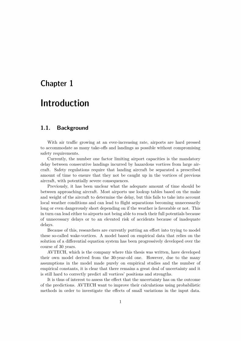
2.3.1. Vortex MovementLet ri = (x, yi, zi) denote the position of a vortex i, let Bi be its buoyancy factor,

let W be the wind with

W(x, y1, y2, z1, z2) = 12(W(x, y1, z1) + W(x, y2, z2)

)being its average value as defined in Section 2.2.1, and let vi be the Biot-Savartinteraction-velocity (see below). Then vortex i’s spatial time-derivatives are givenby:

dx

dt= W(x, y1, y2, z1, z2) · ex (2.21)

dyidt

=[vi(. . . ) + W(x, yi, zi)

]· ey (2.22)

dzidt

=[vi(. . . ) + W(x, yi, zi)

]·Bi(t)ez. (2.23)

For brevity, we omitted the arguments to vi and replaced them by ’. . . ’ because,as we will see in the next section, vi depends on all vortex positions ri and vortexstrengths σi.

However, Formulae (2.21)-(2.23) can be further simplified. Since W(. . . ) ·ez = 0by definition (Section 2.2.1) we get the simpler system:

dx

dt= W(x, y1, y2, z1, z2) · ex (2.24)

dyidt

=[vi(. . . ) + W(x, yi, zi)

]· ey (2.25)

dzidt

= vi(. . . ) ·Bi(t)ez. (2.26)

Note that dxdt is lacking a subscript because, as was mentioned, all vortices share

x-coordinate with the gate.

2.3.2. Biot-Savart InteractionsWe mentioned that vortices affect each other through the so-called Biot-Savart

interactions. They work as follows: The effect one vortex has on another vortex’svelocity is proportional to the strength of the affecting vortex, and inversely propor-tional to the distance between them. That is, the velocity contribution from vortexj to vortex i is given by:

vij = σj(t, . . . )eij × exrij

(2.27)

12


where σj is the circulation strength of vortex j. It is closely related to the circu-lation function Γ(t) from Section 2.2.2, but its exact definition will have to waituntil Section 2.3.3 because it depends on the vortex. The unit vector eij pointsfrom vortex j to vortex i. Equation (2.27) is called the Biot-Savart law applied toaerodynamics and is further explained in Rytter [1]. Moreover, vortex i will be af-fected by all other vortices in the simulation, so the total ‘Biot-Savart contribution‘experienced by vortex i is thus:

vi =∑j 6=i

vij . (2.28)

That is, the sum of the contributions from each individual vortex.

Special Case - Out of Ground

We do not explicitly calculate the Biot-Savart interactions if there are onlytwo vortices participating in the simulation. This is because the vortices are thenassumed to be fixed relative to each other, which allows us to use a different formula:

vi =[1− exp(−(0.4b0)21.257

rc(Γ(t))2 )]ez (2.29)

where rc is the so-called effective core radius. It was first introduced by Holzäpfel[2], and is given implicitly by:

Γ5−15(t) = Γ5−15(t = 0)11

15∑r=5

[1− exp(−1.257(r/b0)2

rc(t)2 )]. (2.30)

By equating Equation (2.30) and Equation (2.19) one can find rc as an implicitfunction of Γ.

Equation (2.29) is related to Equation (2.27), but uses the fact that the vortexpair has a fixed separation when descending together. A simulation with only twoactive vortices is known as Out of Ground Effect, see below.

The rest of this chapter will be devoted to explaining the ground effects.

2.3.3. The Ground EffectsAs mentioned, there are different phases of the model. For historical reasons,

we call these phases ground effects. Ground effects are intended to capture the factthat vortices behave differently depending on which altitude they are generated.Thus, different ground effects will be present on different altitudes. Vortices do notnecessarily need to go through all of the phases during their lifetime. For instance,a typical scenario for vortices that originate close to the ground is that they willnever enter Phase I but instead start in Phase II or III .

Generally, the rule is that the closer to the ground the more complex the groundeffect you have to use. This is because the proximity to the ground will require the

13


addition of secondary vortices that change the behavior of the system. We willclarify how secondary vortices work when describing In Ground Effect, see below.

In addition to secondary vortices, another key concept in explaining the groundeffects is the concept of mirror vortices. Mirror vortices are imaginary vorticesintroduced below ground-level in the simulation with the purpose of stopping theirreal companions from falling through the ground. A mirror vortex always has thesame y-coordinate as its companion but a z-coordinate of opposite sign. It alsoalways rotates in the opposite direction of the vortex it is mirroring.

h

h

Figure 2.5. Illustration of a mirror vortex. It has the same altitude as its realcounterpart, except that its sign is negative. Also, the mirror vortex rotates in theopposite direction.

The ground effects will be presented in ascending order of complexity. Thus,Effect I is the simplest and operates at the highest altitude. In the P2Pm modelthere are three distinct effects. The first two of these are analogous to Phase I andPhase II of NASA [4] respectively, whereas the third one corresponds to Phases IIIand IV.

Note however that since there are only three effects, it will be easier to assign adescriptive name to each of them rather than referring to them using numbers.

Phase I - Out of Ground Effect - OGE

Out of Ground is active whenever we are modeling the system far above theground. Typically, this will be the ‘fallback‘-effect in the sense that there is noexplicit criterion for when to run this effect. Instead we use Out of Ground whenevernone of the other effects is active.

During OGE there are just the two initial main vortices participating in thesimulation. Because of that, one wants to avoid calculating the Biot-Savart contri-butions and instead uses an explicit formula, as already described in Section 2.3.2.

Figure 2.6 gives a schematic illustration and Figure 2.7 gives an example ofvortex movement during OGE.

Phase II - Near Ground Effect - NGE

Near Ground Effect is initiated once both vortices fall below the predefinedheight h = 1.5. The vortices are not supposed to fall through the ground, so two

14


Figure 2.6. Illustration of Out of Ground Effect. The two vortices are descendingtogether toward the ground.

0 20 40 60 80 100

8

10

12

14

y

z

Figure 2.7. Illustration of a typical vortex time-trajectory during OGE. We seeboth main vortices (there are two graphs, one for each vortex) starting off at z ≈ 15and descending together until their circulation has died after which they just floatwith the wind.

mirror vortices are introduced; one for each real vortex. Each real vortex is affectedthrough Biot-Savart by the three other vortices (the other real one and the twomirror vortices). The result is that the descent of the real vortices slows downand instead they are pushed apart along the y-axis. Figure 2.8 illustrates the ideabehind NGE.

NGE is a ‘transition‘ ground effect, i.e, vortices seldom stay in NGE during awhole simulation. For instance, in Figure 2.2, the vortices start in Out of GroundEffect, transition to Near Ground Effect when they fall below z = 1.5 and finallyalso enter In Ground Effect (can be seen in the figure as the point when they startmoving upwards). Note, however, that it is very hard to visually distinguish NGEin Figure 2.2.

15


Figure 2.8. Illustration of Near Ground Effect. The two vortices are approachingthe ground and give rise to two mirror vortices below ground level. The effect of themirror vortices is to slow down the vertical movement and also to push the vorticesapart along the y-axis.

Phase III - In Ground Effect - IGE

In Ground Effect is by far the most complicated effect. There are differentcriteria for each main vortex to initiate IGE. Let

Wydef= W · ey (2.31)

be the y-component of the mean wind defined in Section 2.2.1. For the first primaryvortex the criterion is

z ≤ Z1def=

1.0 Wy ≤ −10.6− 0.4Wy −1 < Wy < 00.6 0 < Wy

(2.32)

For the second primary vortex we have similarly

z ≤ Z2def=

0.6 Wy < 00.6 + 0.4Wy 0 < Wy < 11.0 1 ≤ Wy

(2.33)

These conditions are intended to emulate the so-called adapted rebound, where thewind causes the vortices to enter IGE at different heights. It is further discussed inRytter [1].

Once a main vortex has entered IGE it will stay in that state. When just onevortex is IGE the other vortex will give rise to only a mirror vortex while stillinteracting with all the other (mirror) vortices in the simulation.

In IGE we introduce not only mirror vortices, but also secondary vortices thatorbit their main vortex companions. Secondary vortices are virtual. That is, theydo not exist physically, but are there to ’aid’ the real vortices in behaving as theyshould. The result of adding secondary vortices to the simulation is that theywill push the main vortices upward. Every secondary vortex also gives rise to a

16


Figure 2.9. Illustration of In Ground Effect. There are multiple secondary vorticesas well as mirror vortices, causing complex behavior. The secondary vortices areorbiting the main ones, pushing them further up in the atmosphere.

corresponding mirror vortex. In Figure 2.9 we have illustrated IGE. From Figure 2.9it is easy to see why we have mentioned that IGE is the most complex ground effect.Also refer to Figure 2.12 where the characteristic upwards vortex-movement of IGEcan be seen.

There are two secondary vortices to be introduced for each main vortex. Thefirst one is introduced once IGE is entered and the second one is introduced oncethe first one has rotated 180◦ around its main vortex.

When referring to a secondary vortex’s angle α, we mean the angle where α = 0◦corresponds to a position directly below its respective main vortex and α = −90◦positions the secondary vortex between the two main vortices (so α = −90◦ for aleft-side secondary vortex puts it to the right of its main vortex whereas a right-sidesecondary vortex ends up to the left of its main companion), as shown in Figure 2.10.

Let z0 denote the initial altitude of the main vortices, i.e., at time t = 0. Thenthe starting position for every secondary vortex is at an angle of α0 = −45◦ and atthe distance R from its main vortex , where

R ={

0.4 + (0.4/0.5)(z0 − 0.5) z0 < 0.50.4 z0 ≥ 0.5

(2.34)

The strength of a secondary vortex i is different depending on its angle andwhether it belongs to vortex 1 or 2. Let αi be its angle and Wy = W · ey be they-component of the mean wind as defined in Section 2.2.1. Then

σi(t,W) = −f(αi)G1(Wy)Γ5−15(t), i ∈ {3, 5} (2.35)σi(t,W) = f(αi)G2(Wy)Γ5−15(t), i ∈ {4, 6} (2.36)

where

G1def=

0.2 Wy ≤ −10.3 + 0.1Wy −1 < Wy < 00.3 0 < Wy

(2.37)

17


Main vortices

Secondary vortices

Figure 2.10. Illustration of how angles are measured for secondary vortices. In thepicture, both secondary vortices have an angle of approximately 45◦

G2def=

0.3 Wy < 00.3− 0.1Wy 0 < Wy < 10.2 1 ≤ Wy

(2.38)

are factors that emulate the adapted rebound discussed in Rytter [1]. The signdifference in Equations (2.35) is due to the fact that secondary vortices rotate in theopposite direction of their primaries. The function f(α) was introduced in NASA [4](where it is called ‘thetafac‘) in order to model the fact that the secondary vorticesaffect their primary companions differently depending on their relative angles. Thefunction f(α) is defined as the piecewise linear 360◦-periodic function given byFigure 2.11 below.

Note also that the σi possess a property we will be using in Chapter 6: they onlydepend on the wind during weak cross-wind. That is, G1 and G2 are both constantwhenever |Wy| ≥ 1. As long as that condition holds we can be sure that the windwill not affect σi.

18


−45 45 135 225 315

0

0.2

0.4

0.6

0.8

1

α (◦)

f(α

)

Figure 2.11. Plot of the 360◦-periodic ‘thetafac‘ [4] function f(α).

0 5 10 15 20 25 300

1

2

3

4

5

y

z

Figure 2.12. Illustration of a vortex time-trajectory during IGE. We see both mainvortices influenced by the orbiting secondary vortices (dashed lines), rendering theirtrajectories slightly unpredictable. The vortices start at z ≈ 0.7 and are pushedupward by the secondary vortices.

19

Chapter 3

ODE System

Having described the physical model, we now turn to the task of defining thesystem of ordinary differential equations that will be used to calculate the vortices’movements. The ODE system is quite complex and contains many different statevariables with dissimilar purposes. Therefore, we will start out by constructingsome auxiliary mathematical tools that will simplify the presentation of the system.

In Chapter 2 we explained that the vortex coordinates can be referred to by e.g.

ri = (x, yi, zi) (3.1)

where i is the number assigned to a specific vortex, see Table 2.1. From now on wewill also need to refer to the coordinates of the mirror image of vortex i. These willbe denoted r′i and are defined by:

r′i = (x, yi,−zi). (3.2)

Also let r′ij denote the vector from the mirror of vortex j to vortex i:

r′ijdef= ri − r′j (3.3)

3.1. Mathematical DefinitionsAs mentioned previously, we want to make some mathematical definitions in

order to allow the ODE to be formulated more elegantly. For instance, we will beable to ‘encode‘ each ground effect condition using mathematical expressions. Indoing this, we will make heavy use of the Heaviside function, which we will denoteby H(x). Its definition is

H(x) ={

0 x < 01 x ≥ 0.

(3.4)

The Kronecker delta δij will also be important:

δij ={

1 i = j

0 i 6= j(3.5)

21

CHAPTER 3. ODE SYSTEM

Ai

vOGEi

Z1, Z2

ε

vij

vi

S

f(α)

N

vBSi

I1, I2

N

t

W1,W2

xyi αizi

σi

Γ

Figure 3.1. Graph of all the dependencies of the intermediate functions defined inSection 3.1.

Figure 3.1 provides an overview of all the functions that will be defined in thissection and how their interdependencies work.

3.1.1. The Vortex Index Functions

Table 2.1 displays the numbering scheme used for the vortices. It will oftenbe the case that certain functions are the same for all left-side vortices, and viceversa on the right-hand side. It will therefore be useful to translate a vortex’s indexnumber to its corresponding main vortex‘s index number.

Define the function m : {1, 2, ..6} → {1, 2} to be the map from each vortexindex to the corresponding main vortex index for that side. That is, left-side vortexindices are mapped to 1 and right-side ones are mapped to 2. Using the enumerationfrom Table 2.1 we can formulate this as

22

3.1. MATHEMATICAL DEFINITIONS

m(i) ={

1 if i is odd2 if i is even (3.6)

This will allow us to define e.g. only G1, G2 below instead of G1, G2, G3, . . . , G6because G1, G3, G5 would all be the same.

Furthermore, lets(i) = m(i) + 2 (3.7)

so that s(i) is the index of the first secondary vortex on the same side as vortex i.

3.1.2. Representing the Z and G functionsUsing the Heaviside-function, we can define mathematical expressions for Zi and

Gi that we discussed in Section 2.3.3, specifically in Equations (2.35) and (2.37)-(2.38).

Z1 = 0.6 + 0.4H(−Wy)[|Wy|H(1− |Wy|)− (|Wy| − 1)H(|Wy| − 1)

](3.8)

Z2 = 0.6 + 0.4H(Wy)[|Wy|H(1− |Wy|)− (|Wy| − 1)H(|Wy| − 1)

](3.9)

G1 = 0.3− 0.1H(Wy)[|Wy|H(1− |Wy|)− (|Wy| − 1)H(|Wy| − 1)

](3.10)

G2 = 0.3− 0.1H(−Wy)[|Wy|H(1− |Wy|)− (|Wy| − 1)H(|Wy| − 1)

](3.11)

As we see, these are all functions of the mean wind, which depends on x, y1, y2, z1and z2.

3.1.3. The Ground Effect ConditionsGiven the complex logic for determining e.g. when In Ground Effect is active,

we will formulate indicator functions that will be 1 whenever the conditions aresatisfied and 0 otherwise.

We denote the NGE-condition function by N (z1, z2) (not to be confused withthe stratification Ni(x, yi, zi)) and define it:

N (z1, z2) = H(h− z1)H(h− z2) (3.12)

which thus evaluates to 1 only when both main vortices are below h, in accordancewith Section 2.3.3. Note that N will evaluate to 1 even when the vortices havefallen so low that IGE should activate.

The task of writing an indicator function for IGE is a little bit trickier. Remem-ber that both main vortices can enter IGE independently. Thus we will have todefine two indicator functions; one for each side. Another caveat is that the logicfor IGE states that we should not ever leave IGE once it has commenced. Since

23


the Biot-Savart interactions in IGE invariably cause the vortices to move relativeto each other, we can restate that condition as ‘the secondary vortices have rotatedaway from their initial positions‘. Thus, let α3 and α4 represent the secondaryvortex angles of vortices 3 and 4 respectively. Then the IGE indicator functions are

I1(x, y1, y2, z1, z2, α3) = H(H(Z1 − z1) + α3 − α0) (3.13)I2(x, y1, y2, z1, z2, α4) = H(H(Z2 − z2) + α4 − α0). (3.14)

where α0 = −45◦ is the initial angle of the secondary vortices. The I1, I2-functionsare 1 only if it the secondary vortex angles changed or if the vortices are under theirrespective altitude-threshold for initiating IGE. See Section 2.3.3.

Finally, we will also need an expression for when the second secondary vorticesactivate:

S1(α3) = H(α3 − 180◦ − α0) (3.15)S2(α4) = H(α4 − 180◦ − α0) (3.16)

that is, we are checking ‘has the first secondary vortex rotated 180◦ relative to itsinitial angle α0 yet?‘.

3.1.4. The Vortex Circulation StrengthsThe vortices have different circulation strengths depending on whether they are

secondary or not, and depending on which side they are on. It will be cumbersometo write out each vortex’s circulation directly in the ODE. Hence, we define thefunctions σi representing the circulation strength of each vortex i:

σi(t, x, y1, y2, z1, z2, α3, .., α6) = (−1)iΓ(t)×{

1 i ≤ 2f(αi)Gm(i) i > 2

(3.17)

where the factor (−1)i represents the fact that left and right vortices rotate inopposite directions. The αi are the secondary vortex angles introduced above. Thefunction f(α) used here is the ‘thetafac‘-function, see Figure 2.11. The map m(i)was defined in Section 3.1.1 and Γ(t) is the Γ5−15(t) of Section 2.2.2.

3.1.5. The Vortex Activation FunctionsDifferent vortices have different conditions for when they are to activate. Just

as for circulation strength, it is cumbersome to incorporate this logic directly intothe ODE formulation. Thus, let

Ai(x, y1, y2, z1, z2, αs(i)) =

1 1 ≤ i ≤ 2

Im(i) 3 ≤ i ≤ 4Im(i)Sm(i) 5 ≤ i ≤ 6

(3.18)

be indicator functions evaluating to 1 whenever their respective vortices are toactivate. The αi, Ii and Si were all defined in Section 3.1.3.

24

3.2. FORMULATING THE ODE SYSTEM

3.1.6. The Biot-Savart TensorsThe Biot-Savart interactions were explained in Section 2.3.2. Now that we have

made suitable definitions for denoting vortices and their circulation strength, we areready to define vij . Its definition will be very similar to that of the physical model:

vij = vij(x, yi, yj , zi, zj) = σj(. . . )rij|rij |2

× ex (3.19)

where σj was defined in Section 3.1.4 and the notation rij was discussed in the begin-ning of Chapter 2. However, we also have to deal with mirror vortex contributions.As such, let

v′ij = v′ij(x, yi, yj , zi, zj) = −σj(. . . )r′ij|r′ij |2

× ex (3.20)

represent the contribution from the mirror of vortex j to vortex i. The minus sign isthere because mirror vortices rotate in the opposite direction of their companions.

Just as in the physical model, vi will be the total Biot-Savart contribution tovortex i. However, because of the special case in OGE (see Section 2.3.2), theexpression will be a little more complicated than in Section 2.3.2. We have todefine it so that it chooses the right vi depending on the prevailing Ground Effect.Let N be the NGE indicator function that was defined in Section 3.1.3. Then

vi = NvBSi + (1−N )vOGE

i . (3.21)

where

vBSi =

6∑j=1

Aj

((1− δij)vij + v′ij

)(3.22)

vOGEi =

[1− exp(−(0.4b0)21.257

rc(Γ(t)) )]ez. (3.23)

We neglected to write out all the dependencies above because it would clutter upthe notation. In fact vi depends on all coordinate pairs (yk, zk) where k is an indexof an active vortex. If k is an index of a secondary vortex, then vi will also dependon its secondary angle αk as discussed in Section 3.1.4. Furthermore, vi dependson the time t and the x-coordinate of the gate (explained in Section 2.1).

We used the Kronecker delta in Equation (3.22) to omit the term vii which isundefined. The Aj is meant to filter out vortices that are inactive.

3.2. Formulating the ODE SystemWe have made all the definitions that we need. We will now show how to

construct the ordinary differential equation that incorporates the information inthe physical model and describes wake-vortex movement.

25


It can be very difficult to get a good overview of the ODE we are about todescribe because of the many different variables with dissimilar purposes. Thus wewould recommend the reader to consult Figure 3.2 below, were we have tried tovisualize all the direct inter-variable dependencies.

As has been already stated, the system we formulate is a standard OrdinaryDifferential Equation:

u = f(u, t) (3.24)with the state vector

u =

xB1B2α3...α6y1z1...y6z6

(3.25)

where the dot in the left-hand side denotes a time-derivative and t denotes time.We will attempt to give physical meaning to the state vector u, and define the

function f(u, t) component-wise.

3.2.1. The x-Coordinate of the GateDenoted by x. The time-derivative x is only affected by the wind. Hence it is a

function of the main vortices y- and z-coordinates as well as of x.

x = W(x, y1, y2, z1, z2) · ex (3.26)that is, it is equal to the x-component of the mean wind vector W defined inSection 2.2.1. As mentioned in Chapter 2, each vortex will have the same x-position.

3.2.2. The Buoyancy FactorsDenoted by B1 and B2. The buoyancy factors are functions of the main vortex

positions and also of the vector vi. For i ∈ {1, 2}:

Bi = 181400N(x, yi, zi)2

√2(z0 − z). (3.27)

That is, Equation (3.27) is the same as Equation (2.20).Even though there can be up to 6 vortices there will only be two buoyancy

factors; one for each main vortex. The rationale is that the secondary vortices are

26


vij

αi

αi

Ai

Bi

I1, I2

ziyix

N

S

W1,W2 ε

Z1, Z2 Γ

vOGEi

f(α)

vBSi

Bi

N

t

vi

yixzi

σi

Figure 3.2. Graph showing how the ODE variables depend on the intermediatefunctions and on each other. It contains the graph of Figure 3.1 as a subgraph. Notethat the graph is so complex because it incorporates the dependencies of each groundeffect. For ground-effect-specific dependency-graphs, see the end of this chapter.

merely supposed to ‘aid‘ their corresponding main vortex. They are not real physicalvortices and as such should use the same buoyancy factor as their counterparts inorder to follow their motion.

27


3.2.3. The Secondary Vortex AnglesSecondary vortices were explained in Section 2.3.3. We introduce one angular-

variable per secondary vortex so that we can e.g keep track of when they have rotated180◦ (see Section 2.3.3). There are thus four secondary vortex angles, but we willsubscript them with the number of the particular vortex they are representing. Thusthe variables are: α3, α4, α5, α6, c.f Table 2.1.

For i ∈ {3, 4, 5, 6} we have:

αi = Ai(x, y1, y2, z1, z2, αs(i))rm(i) i × (vi − vm(i))

|rm(i) i|2(3.28)

which is a standard formula from solid mechanics for calculating angular velocity,multiplied by the IGE indicator function. Notice that vi − vm(i) is the relativevelocity of vortex i with respect to its main vortex.

Remark on Redundancy

As explained in Section 2.3.3, during IGE a second secondary vortex is to beintroduced once the first secondary vortex rotates 180◦ around its main companion.This requires us to somehow keep track of the secondary vortices’ angles throughouta simulation. We do this by introducing one angular variable per secondary vortex.Since we also save each vortex’s y- and z-coordinates this creates some redundancy.

Had we saved a radius r per secondary vortex we could just calculate y andz instead. Thus it is in fact possible to formulate the same ODE with a smallernumber of variables. However, for our purposes the numerical solution time is mostimportant, and the alternative approach requires more trigonometric computations,which would detract from the possible gains of reducing the variable count.

3.2.4. The Vortex Coordinate PairsJust as in Section 2.3.1, let

yi =[vi + W(x, yi, zi)

]· ey (3.29)

zi = vi · ezBi (3.30)

for the main vortices, i.e, for i ∈ {1, 2}.When dealing with the secondary vortices, the equations become slightly more

complicated. The secondary vortices need to follow the movement of their maincounterparts until the moment when they themselves become active. Furthermore,they use the same wind as their main vortices [1]. Thus, for i ∈ {3, 4, 5, 6},

yi =[Aivi + (1−Ai)vm(i) + W(x, ym(i), zm(i))

]· ey (3.31)

zi =[Aivi + (1−Ai)vm(i)

]· ezBm(i) (3.32)

28


Simplification During OGE

Consider the y- and z-derivatives defined above. Equations (3.21) and (3.23)show that during OGE, vi · ey = 0. Hence for i = 1, 2, these formulae hold:

yi = W(x, yi, zi) · ey (3.33)zi = vi(t, . . . ) · ezBi(t) (3.34)

Or, by inserting from (3.23):

yi = W(x, yi, zi) · ey (3.35)

zi =[1− exp(−(0.4b0)21.257

rc(Γ(t)) )]Bi(t) (3.36)

We will make use of this simplification in Chapter 6.

3.2.5. Initial ValuesGiven an initial height z0 to run the simulation on, the initial values are as

follows:

u0 =

xB1B2α3...α6y1z1y2z2y3z3y4z4y5z5y6z6

=

011α0...α0−0.5z00.5z0

−0.5−R sin(α0)z0 −R cos(α0)0.5 +R sin(α0)z0 −R cos(α0)−0.5−R sin(α0)z0 −R cos(α0)0.5 +R sin(α0)z0 −R cos(α0)

(3.37)

The initial vortex angle α0 = 45◦ and R were explained in Section 2.3.3.Note that the initial conditions are invariant with respect to aircraft size, as

explained in Section 2.1.

3.2.6. Ground Effect-Specifc DependenciesPart of the complexity in the ODE seen in Figure 3.2 comes from the fact that

it must be able to switch ground effects. Had we dealt with each effect separately,

29


the graphs would have looked simpler, as shown in Figures 3.3, 3.4 and 3.5. Thetask of formulating a new model that treats each ground effect as a separate ODEis suggested as a future development in Section 7.2.

vOGEi

Bi

Bizi yi x

N

αi

t

W1,W2ε

yixzi

Γ

Figure 3.3. Graph of all dependencies during OGE. Note that αi = 0 always, whichis why it is depicted by an isolated node.

30


Bi

ε

Bi

vij

ziyix

N

vBSi

αi

t

W1,W2

vi

yixzi

σi

Γ

Figure 3.4. Graph of all dependencies during NGE. Note that αi = 0 always, whichis why it is depicted by an isolated node.

31


vij

αi

αi

Ai

Bi

ziyix

N

S

W1,W2 ε

Γ f(αi)

vBSi

Bi

t

vi

yixzi

σi

Figure 3.5. Graph of all dependencies during IGE.

32

Chapter 4

Implementation

We have defined the physical model and showed how to represent it using anODE. We will now describe how the ODE is solved numerically. Due to the intentionof performing Monte Carlo-simulations, the algorithm that we use needs to executequickly. In fact, emphasis has been given to speed over accuracy, seeing as weare more interested in studying how the solution changes as a result of the MonteCarlo-variations than in the accuracy of any single solution.

4.1. Solving on the Graphics CardGPUs excel at performing arithmetic-intense calculations in parallel. The IVPs

we wish to solve are all independent, and as such are excellent candidates for par-allelization. The numerical scheme is therefore implemented on the GPU using theOpenCL-toolkit.

It should be pointed out that there are multiple ways of achieving parallelismfor the problem we are trying to address. For instance, one might attempt toparallelize even the solution of a single IVP, e.g. by calculating each ODE-variablein a parallel thread of execution. The difficulty in this approach, lies in the factthat the variables are far from independent, as is evident from Figure 3.2. The taskof achieving parallelism using this approach is thus clearly nontrivial, and is notattempted in this thesis.

4.2. Solver AlgorithmThe Runge-Kutta4 (RK4) algorithm is employed to solve the IVPs. It is a well

known method of order 4. Note that the implementation uses a fixed stepsize, eventhough it is possible to write an adaptable RK4 algorithm.

Nevertheless, as we will see in Chapter 5, the main reason for low accuracy in thesolution is not due to the algorithm itself but because of discontinuities within theODE. It is true that an adaptive scheme would be able to bypass this problem byreducing the stepsize repeatedly until the exact point of the discontinuity is found.

33

CHAPTER 4. IMPLEMENTATION

However such a process would require a large overhead due to having to reevaluatethe points close to a discontinuity so many times.

Additionally, by employing an adaptive scheme, one would run the risk of losinghomogeneity. Meaning that solving different IVPs in the Monte Carlo-simulationmight require different stepsizes, which in turn requires branching. That would havebad consequences for performance on a GPU device[7].

4.3. The Weather GridWe mentioned in Section 2.2.1 that weather data is supplied by a large weather

grid, from which the weather at any particular position can be calculated throughinterpolation.

The grid consists of several layers. Layers are stacked almost directly on top ofeach other so that corresponding grid points from different layers almost align. By‘almost‘ we mean that the grid is typically constructed from real-world measure-ments, and the position of each measurement can be off by a couple of meters.

Typically, the layers are vertically separated by approximately 300 m, and gridpoints of the same layer tend to be approximately 10 km apart.

Prior to a simulation, the weather grid is queried for weather data in the areathat the simulation is to figure in. A query for weather data usually results in threesets of grid points; two sets of points from the closest layers below the requestedposition, and another set of points for the closest layer above it.

Each grid point contains information about the wind vector, turbulence andstratification at that position. The wind vector at a specific point within the grid iscalculated as a weighted average of all the requested grid points, where the weightis taken to be the reciprocal of the squared distance to each point. Thus, if we callthe k requested grid points p1,p2, ...,pk we can write the formula for the wind ata specific point p = (x, y, z):

W(x, y, z) =

∑ki=0

W(pi)|p− pi|2∑k

i=01

|p− pi|2

(4.1)

In contrast, turbulence is calculated as a standard average across all grid points.The reason is that turbulence affects the vortex circulation. If it were allowed tochange as a function of position, the circulation would no longer be guaranteed tobe continuous. Thus turbulence E has the formula:

E =k∑i=0

E(pi)k

(4.2)

As for the stratification, we will actually have two different formulae. Therationale is that stratification, just as turbulence, affects vortex lifetime and as such

34

4.4. THE MEMORY SETUP

must be kept constant in the circulation formula. Thus the circulation function usesthe constant stratification:

Ncirculation =k∑i=0

S(pi)k

(4.3)

However, the other use of stratification is in the buoyancy factors, and in thiscase we really want its value to vary. Thus in this case we employ the weightedaverage:

Nbuoyancy(x, y, z) =

∑ki=0

S(pi)|p− pi|2∑k

i=01

|p− pi|2

(4.4)

Finally, in order to use the weather data within the ODE one must convert itto use the local coordinate system. This includes rotating the wind according to itsrelative bearing to the gate, as well as converting to use the right units [1]:

W [length units/time units]← b0/t0W [ms−1] (4.5)N [time units]← Nt0 [s−1] (4.6)

ε [length units2/time units3]← ε2t0b0 [m2s−3]. (4.7)

4.4. The Memory SetupWe now explain the memory setup in the implementation. Choosing a memory

setup has performance implications. For instance, excessive use of global memoryshould be avoided when other, faster memory types are available. It is neverthelessnecessary to use global memory occasionally because it is the only memory typesuitable for storing large amounts of data. Note that this discussion will require someunderstanding of the OpenCL memory types: private, local, global and constant.For information on these, see e.g. Gaster et al [5].

4.4.1. Weather Grid Data

Weather data is stored in constant memory since it is shared throughout allconcurrent simulations. Each weather point requires six parameters: wind strength,wind direction, stratification and position (x, y, z). The total required amount ofmemory using single precision storage is thus

(1 + 1 + 1 + (1× 3)

)× 4 = 24 bytes.

As there are typically around 10 weather points per Monte Carlo-simulation thisrequires a total of approximately 240 bytes. The small amount of memory requiredmakes it perfect for storage in constant memory.

35


4.4.2. Simulation ParametersThis is data specific to a single initial value problem. Thus the memory re-

quired for this data grows linearly as a function of the number of simultaneous sim-ulations. Presently, the simulation parameters include the precomputed constantsν1, ν2, T1, T2 and also some parameters for the Monte Carlo-simulations: turbulenceperturbation, stratification perturbation, wind strength perturbation and wind di-rection perturbation. Thus a total of (1 × 8) × 4 = 32 bytes per Initial ValueProblem.

The simulation parameters reside in constant memory. However, there is noparticular reason for storing them there, except for the fact that they are constant.They could just as well be stored in other memory types. For a thousand simulationsin total, the memory requirements start approaching the maximum capacity ofconstant memory for some OpenCL implementations. So in order to increase thenumber of simulations, one would likely have to relocate this data elsewhere.

4.4.3. Runtime ParametersThese are parameters that are constant throughout a whole Monte Carlo-simulation,

just like the weather data. They include only three parameters of which only onepertains to the physical model itself (the rest are implementation-specific constantsrequired e.g. for storing memory at correct addresses). Thus it requires approxi-mately 12 bytes and can easily be stored in constant memory.

4.4.4. The Solution DataThe solution data is a large buffer allocated in global memory where all the par-

allel solutions can be written. Typically, the GPU was given approximately 1000IVPs at a time to solve. Thus, 19 variables per 1000 executions per approximately900 time steps requires around 9 MB. Note that if increasing the number of simul-taneous executions one will have to break this buffer into smaller chunks becausesome graphics cards (and OpenCL enabled CPUs) have a maximum limit on thesize of a continuous chunk in global memory.

4.5. Accuracy vs Performance Trade-offsSeeing as the purpose is a Monte-Carlo simulation, and that the maximum error

is allowed to be fairly large (see Section 5.4), a number of performance optimizationsare employed in order to gain execution speed.

4.5.1. Native MathThe GPU‘s native implementations of common math functions are used in favor

of the standard math library. These are accessible in OpenCL using the prefix‘native_‘, e.g. ‘native_exp‘ or ‘native_cos‘.

36

4.6. GPU IDIOSYNCRASIES

4.5.2. An rc(Γ(t))-Lookup TableThe computations in OGE feature the calculation of an implicit function, namely:

rc(Γ(t)).

This is a relatively costly operation to the otherwise very simple OGE formulae, seeSection 2.3.2. Thus, we use a lookup table to gain speed, as in Rytter [1].

Note, however, that the type of interpolation can impact the accuracy of thealgorithm, since it relies on the fact that the integrated function is continuous anddifferentiable.

4.5.3. CirculationThe circulation is given in (2.10) as an integral. However, in the implementation,

we approximate the integral by a relatively crude Riemann sum:

Γ(t) ≈ 111

15∑r=5

Γ(r/b0, t) (4.8)

The same ‘optimization‘ is performed in both Rytter [1] and Holzäpfel [2].

4.6. GPU IdiosyncrasiesThere were a number of interesting obstacles encountered throughout the devel-

opment of the numerical scheme which pertain to the fact that we are developingon a GPU. It would be worthwhile to outline them here so that future work neednot repeat the same trouble-shooting.

4.6.1. Debugging on the GPUAt the time of writing, there is practically no available support for debugging the

OpenCL code. Some error reporting can be achieved by specifying slightly largerdifferential equation system than required. For instance, we require 19 variables toformulate the ODE, but when implementing, 24 variables can be used instead so asto have 5 variables that the numerical scheme completely ignores but that could beuseful for outputting various data that could be helpful in trouble-shooting.

4.6.2. Vectorization SpeedupsModern GPUs and CPUs support so called Single Instruction Multiple Data

(SIMD) operations, which allow for a single thread to do many computations inparallel. OpenCL supports these operations through the use of its vector datatypes,e.g. float4, f loat16 etc.

It was found that the recommended approach to using these kinds of operationsvaries depending on the device. For instance, Intel [10] recommends that vector

37


operations be explicitly used as much as possible, whereas NVIDIA recommendsthat they only be used at leisure. From NVIDIA OpenCL Best Practices [7], chapterInstruction Optimizations:

[...] The CUDA architecture is a scalar architecture. Therefore, there isno performance benefit from using vector types and instructions. Theseshould only be used for convenience. [...]

It should be pointed out that using vector operations in the ODE appeared toincrease CPU performance but to decrease it on the GPU.

4.6.3. Floating Point AccuracyPresently, even the most cutting edge GPUs struggle with double precision arith-

metic efficiency, and single precision accuracy can be orders of magnitude faster[6].Therefore, NVIDIA recommends that single-precision arithmetic be used at alltimes[7]. However, single precision accuracy means that the numerical analysisof the ODE becomes more difficult, e.g. because we get round-off errors. This isimportant to bear in mind, especially in applications where numerical stability is ofthe essence. It might therefore be worthwhile to define something like

#if SINGLE_PRECISIONtypedef float real;

#elsetypedef double real;

#endif

and using real throughout all OpenCL code so as to easily be able to change precisionfor doing e.g. convergence studies.

4.6.4. Data TransferOne has to keep in mind that everything the GPU calculates will have to reside

in GPU memory, which is separate from the RAM accessible to the CPU. Beforestarting execution, one must thus transfer all initial data, including physical pa-rameters and weather data, to the GPU. Once the solutions have been computed,one must also either transfer all the solutions back to main memory or carry outall necessary work on the GPU. It can be preferable to run code on the GPU whichwould run equally fast (or even faster!) on the CPU simply due to the data transferoverhead and lack of parallelism [7].

In our case, we are interested in e.g. computing the mean and variance of all thesolutions. This is a typical instance were it is more efficient to do the work on thegraphics card. That is, instead of transferring all the solutions to the main memoryand then performing the calculations in serial on the CPU, we can parallelize thecomputations and then just transfer the results, saving both execution- and transfer-time.

38

4.6. GPU IDIOSYNCRASIES

4.6.5. Memory Buffer LimitationsIt was discovered that even though modern GPUs can have up to 4 GBs of

memory, there is still a restriction on the size of a contiguous memory buffer. Thusit is not quite as straight-forward as one might think to increase the number ofconcurrent threads. Presently, the required number of threads that are enqueuedon the GPU (one thousand), appears to be just enough so that the solutions canfit nicely inside a single buffer in GPU memory. However, simply increasing thenumber to 10 000 will not work unless one splits up the solution buffer into say 10different parts.

39

Chapter 5

Analysis of the Rate of Convergence

Above, we described the implementation of an RK4-algorithm. RK4 should, byvirtue of being a fourth order method, have an absolute error proportional to thestepsize to the fourth power. We will now discuss under which circumstances thisholds true when solving the wake-vortex ODE.

In performing the numerical convergence studies in this chapter, we have inves-tigated how the solution converges to a reference solution. That is, we compute ahigh accuracy solution and use that as a good approximation of the ’true’ solution,so that we can compute the absolute error of less accurate solutions e.g by taking theabsolute value of the difference from the reference solution. The reference solutionsall have a timestep of approximately 1× 10−2 time units.

Note that in using a reference solution, we can only ever give reasonable ap-proximations of the absolute error for cases when the numerical solution converges.There is no way of telling how great the error is when there is no convergence,because in that case the reference solution is not a good approximation of the exactsolution.

The RK4-algorithm assumes that the differential equation be at least 5th orderdifferentiable [8]. It is not clear that this condition is satisfied under all circum-stances by the wake-vortex ODE, and this is the reason why the theoretical rate ofconvergence cannot always be achieved.

Also, note that the existence and uniqueness of any ODE, y = f(t, y), can only

ε 0.143N 0.700wind strength 2.000wind bearing 228.2◦gate bearing 298.6◦

Table 5.1. The values of the parameters during the convergence study. There is asingle value given per atmospheric property. In other words, all points in the weathergrid have the same value and the weather will be constant.

41

CHAPTER 5. ANALYSIS OF THE RATE OF CONVERGENCE

be guaranteed when f(t, y) is continuous in t and Lipschitz continuous in y [9]. If fis discontinuous, solutions may not exist, but nevertheless they often do. Given thatwe are modeling a physical phenomenon it appears likely that there is a well-definedsolution to the wake-vortex ODE.

Within the ODE, all ground effect transitions generally cause problems. Sincethe ODE changes behavior abruptly once the vortices fall below the altitude-thresholdfor a new effect, there will be discontinuous derivatives that disrupt the convergence.

For instance, when changing from NGE to IGE, we will see discontinuities inthe derivatives of the secondary vortex angles, which throughout NGE have alwaysbeen 0. This causes slower convergence in the angles, which quickly propagates tothe rest of the variables through the Biot-Savart interactions. Figure 5.1 illustratesthat the rate of convergence suffers as a result.

10−2 10−110−7

10−6

10−5

10−4

10−3

10−2

10−1

100

Timestep size (s)

Estim

ated

absolute

Errorinz 1

Theoryt = 64 st = 128 st = 192 s

Figure 5.1. Slow convergence in a simulation that transitions from NGE to IGE.Note that since convergence is so slow, the approximation of the absolute error cannotbe trusted. See the discussion in the beginning of this chapter.

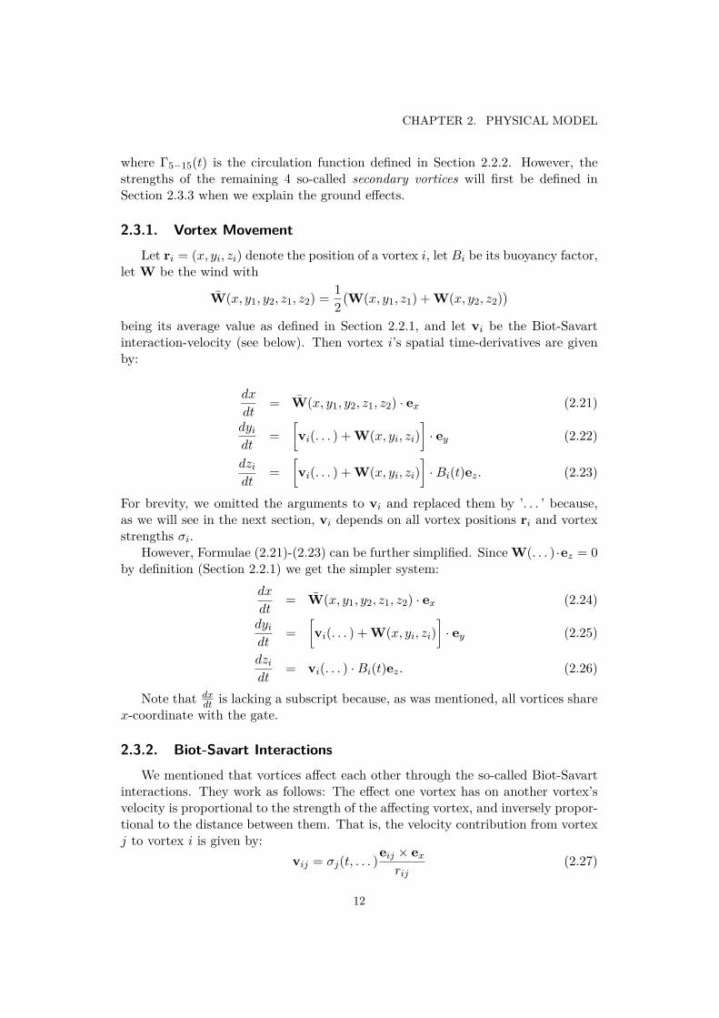
Likewise, when changing from OGE to NGE the vortices will suddenly start torepel in the y-direction whereas previously the y-derivatives were zero (disregardingthe wind), causing slower convergence, as shown in Figure 5.2.

There are also a number of ground-effect-specific issues to be discussed below.

5.1. Convergence in Out of Ground EffectThe ODE has a relatively simple structure during OGE, as can be seen from

Equations (3.35)-(3.36), i.e.,

yi = W(x, yi, zi) · ey (5.1)

zi =[1− exp(−(0.4b0)21.257

rc(Γ(t)) )]Bi(x, yi, zi) (5.2)

42

5.2. CONVERGENCE IN NEAR GROUND EFFECT

10−2 10−1

10−10

10−8

10−6

10−4

10−2

Timestep size (s)

Estim

ated

absolute

Errorinz 1

Theoryt = 64 st = 128 st = 192 s

Figure 5.2. Slow convergence in a simulation that transitions from OGE to NGE. Wesee that t = 64 s (when OGE is still active) is the only one converging as expected.The other graphs are from after the transition. Note that the estimated absoluteerror for the two non-converging graphs cannot be trusted. See the discussion in thebeginning of this chapter.

Both of these formulae are comprised of smooth continuous functions (the implicitfunction rc(Γ) = Γ−1(Γ(rc)) is continuous by the inverse function theorem). Thuswe should expect to get accurate results. Consult Figure 5.3 where the convergenceis shown.

Note that in Section 4.5.2 we mentioned that the implementation uses lookup-tables and interpolation to compute rc(Γ). The choice of this interpolation willimpact the error convergence. Figure 5.3 displays the convergence when using Her-mite Cubic Splines.

5.2. Convergence in Near Ground EffectIn NGE, the equation system is dominated by the Biot-Savart interactions:

yi =[vi + W(x, yi, zi)

]· ey (5.3)

zi = vi · ezBi. (5.4)

The wind function W(x, yi, zi) should always be smooth since it is a model of aphysical phenomenon. The Biot-Savart speed vi in NGE is given by Equation (3.22):

vBSi =

6∑j=1

Aj

((1− δij)vij + v′ij

)(5.5)

43


10−2 10−110−11

10−10

10−9

10−8

10−7

10−6

10−5

Timestep size (s)

Estim

ated

absolute

Errorinz 1

Theoryt = 64 st = 128 st = 192 s

Figure 5.3. Convergence during OGE. The absolute error appears to behave asexpected by theory.

where A3 = A4 = A5 = A6 = 0 since only vortices 1 and 2 and their mirror imagesare active, as explained in Section 2.3.3. Clearly, vi is a sum, and the summands

vij = σj(. . . )rij|rij |2

× ex (5.6)

andv′ij = −σj(. . . )

r′ij|r′ij |2

× ex (5.7)

are all smooth and continuous (with respect to the state variables). Thus, theequation system consists entirely of continuous functions and we can expect accurateresults. Figure 5.4 illustrates this.

5.3. Convergence In Ground EffectIn Ground Effect features the same set of equations as in Near Ground Effect,

except that there are more vortices participating. However, problems will arisebecause the number of participating vortices increases abruptly. In adding a newvortex to the simulation we destroy the convergence. For instance, by letting A5 = 0change to A5 = 1 in order to activate vortex 5, we are creating a discontinuity inthe fifth summand of Equation (5.5).

Thus, the equation system (5.3)-(5.4) is comprised of discontinuous functionsand Figure 5.5 shows that the accuracy suffers due to this.

Note that by making sure that the sum in Equation (5.5) is never discontinuouswe can achieve just as good convergence as in Near Ground Effect. In Figure 5.6the convergence of a modified version of IGE is shown where vortices 5 and 6 never

44

5.3. CONVERGENCE IN GROUND EFFECT

10−2 10−1

10−12

10−10

10−8

10−6

10−4

Timestep size (s)

Estim

ated

absolute

Errorinz 1

Theoryt = 64 st = 128 st = 192 s

Figure 5.4. Convergence during NGE. Error convergence is adequate.

10−2 10−110−6

10−5

10−4

10−3

10−2

10−1

100

101

Timestep size (s)

Estim

ated

absolute

Errorinz 1

Theoryt = 64 st = 128 st = 192 s

Figure 5.5. Convergence during IGE. Convergence does not agree with theory.Therefore we cannot expect the approximation of the absolute error to be accurate.See the discussion at the beginning of this chapter.

activate. That is, the simulation is run from beginning to end with only vortices 1,2, 3 and 4. As can be seen, this preserves the accuracy of the numerical solution,but at the cost of never being able to change the number of participating vortices.

45


10−2 10−1

10−8

10−6

10−4

10−2

100

Timestep size (s)

Estim

ated

absolute

Errorinz 1

Theoryt = 64 st = 128 st = 192 s

Figure 5.6. Convergence during a modified IGE without second secondary vortices.Convergence is better than in Figure 5.5 because there are no discontinuities in theequation system (5.3)-(5.4) anymore.

5.4. Analysis and Proposed ImprovementsWe have studied how the numerical error behaves as a function of the timestep

when solving the ODE using the RK4-algorithm. The RK4 method works wellfor ODEs without discontinuous derivatives. The wake-vortex ODE can be seenas essentially a set of continuous ODEs that have been ‘joined together‘ with thehelp of the Heaviside function H(x) (see e.g Chapter 3 where we used Heaviside toencode all the logic). Thus, we can only achieve 4th order accuracy as long as weapply the RK4-algorithm at a point where no Heaviside function makes its jump.Seeing as all ground effect transitions are governed by Heaviside functions, thesemust be avoided. Furthermore, it is not practical to solve the In Ground Effectwith RK4 since the activation of secondary vortices within IGE is also governed byHeaviside-logic.

In order to remedy the accuracy problem, the most viable option is to amend theODE itself. For instance, one could introduce smooth transitions between groundeffects and smoothly add secondary vortices. Granted, such an approach wouldchange the model but from a physical point of view it nevertheless makes moresense to represent physical phenomena using continuous functions.

Another option is to implement an adaptive numerical scheme which wouldbe able to traverse the discontinuities in the Heaviside functions without losingaccuracy. However, note that such a scheme would have to repeatedly decrease andrecalculate its stepsize in order to deal with the discontinuities, causing a dramaticincrease in computation time.

46

Chapter 6

Analysis of the Parameter Sensitivity

We have mentioned that the wake vortex model is to be used for simulations ofreal-world situations. We now want to clarify how the outcomes of these simulationsare affected by small variations in the input parameters, so as to estimate the model’ssensitivity to measuring errors.

We will study the effect of four parameters, namely: turbulence ε, stratificationN and the wind vector‘s magnitude |W| and direction W/|W|. Since the mainvortices’ y- and z-coordinates are our main interest we will focus the study on onlythose variables.

We want to draw our conclusions through referring to plots from two sets of sim-ulations with authentic weather data. Both setups use data from Thursday, 06 Sep2012 00:00:00 GMT, but one is from 59◦39'7''N, 17◦55'7''E (Stockholm, Arlanda)whereas the other is from 25◦15'10''N, 55◦21'52''E (Dubai, Dubai International Air-port). All parameters are varied separately, linearly from 0 up to +20%, except forthe wind direction which is varied from 0 up to 10◦ instead. The plots display thedifference (due to the parameter variations) in the left main vortex’s coordinates, y1and z1, versus time. That is, the plots display the difference between a perturbedsolution and a reference (unperturbed) solution:

∆y = yunperturbed1 − yperturbed

1 (6.1)∆z = zunperturbed

1 − zperturbed1 . (6.2)

Each plot displays multiple graphs, where different graphs correspond to perturba-tions of different magnitude for the varied parameter.

All the simulations have a gate bearing of 90◦ and initial vortex separation ofb0 = 26.93 m. IGE simulations run at the altitude 20 m while OGE simulations runat 400 m. Since it is very difficult to run a whole simulation in only NGE, we willnot study that ground effect.

Refer to Table 6 for values of t0, which are simulation-specific and required inorder to convert the weather to the model’s length- and time units, as explained inSections 2.1 and 4.3.

47

CHAPTER 6. ANALYSIS OF THE PARAMETER SENSITIVITY

Simulation Setup t0IGE, Dubai 18.457OGE, Dubai 17.797IGE, Stockholm 18.457OGE, Stockholm 17.797

Table 6.1. Values of t0 for each simulation setup

While plots can be useful in explaining ideas it is impossible to cover all casesthat way. Hence, we will also need to examine the ODE directly to draw moregeneral conclusions. In the analysis, we have chosen to respect the implementationand consider the stratification as two separate functions: N(x, y, z) and Ncirculation.

Furthermore, it will be hard to say anything concrete about the ODE behaviorunless we make assumptions, e.g. on the weather functions. For instance, a usefulassumption is that they only depend on the altitude and not on y or x. Thisassumption is plausible seeing as the vortices move at most a couple of kilometersduring strong wind.

Additionally, we would like to point out that even the altitude-dependenceshould be very weak. That is, in typical scenario, wake-vortices descend onlyapproximately 200 m. From the physical meaning of the weather we know thatsuch small altitude differences do not cause drastic changes in wind direction norstrength.

6.1. Sensitivity in Out of Ground EffectAs was stated above, we need to assume that the weather functions only vary as

a function of z, i.e.,

W(x, y, z) = W(z) (6.3)ε(x, y, z) = ε(z) (6.4)

N(x, y, z) = N(z) (6.5)

Otherwise, the complexity of the equations prohibits us from drawing any qualita-tive conclusions with regards to the variables under study.

Nevertheless, when that assumption holds, Equations (3.35)-(3.36) become:

yi(zi) = W(zi) · ey (6.6)

zi(zi, t) = Bi(t, zi, N(zi))[1− exp(− (0.4b0)21.257

rc(Γ(t, ε,Ncirculation)))]. (6.7)

Figure 6.1 depicts the dependency graph resulting from Equations (6.6)-(6.7). Com-pare it to the original OGE dependency graph in Figure 3.3.

Consulting Figure 6.1 and Equations (6.6)-(6.7) we can draw the conclusion thatzi do not depend on W at all. On the other hand, yi has a direct dependence on W.

48

6.2. NEAR/IN GROUND EFFECT SENSITIVITY

vOGEi

Bi

Bizi yi x

N

αi

t

W1,W2

ε

yi xzi

Ncirculation

Γ

Figure 6.1. Dependency graph of the OGE equations, under the assumption thatEquations (6.3)-(6.5) hold.

As a matter of fact, we see in Figures 6.3 and 6.5 that the dependence is essentiallylinear. That is, the difference between two solutions (yI

i , zIi), (yII

i , zIIi ) with slightly

different winds WIi,WII

i is:

∆yi(t) = yIi(t)− yII

i (t) =∫ t

0(WI

i(z1(τ))− WIIi (z2(τ))) · eydτ ≈ tC (6.8)

where C = WIi(t = 0) − WII

i (t = 0). The approximation in the last step is due tothe presumed weak altitude-dependence of W discussed earlier.

Furthermore, notice in Figure 6.1 that yi depends indirectly on zi. This meansthat yi should, in theory, be affected by perturbations in ε and N (since zi is).However, as Figures 6.2 and 6.4 show, this dependence is so weak in practice thatit can be neglected.

So, in general we can say that wind parameters affect only y whereas circulationparameters affect z.

Figure 6.11 illustrates an OGE-trajectory and how different perturbations affectit. Compare with Figures 6.3 and 6.5.

6.2. Near/In Ground Effect Sensitivity

In NGE and IGE, using the same assumptions as in the OGE-analysis in theprevious section, i.e., that Equations (6.3)-(6.5) hold, the ODE Equations (3.29)-

49


50 100 150 200 250

0

2

4

·10−5

Time (s)

∆y

ε-variation

50 100 150 200 250

0

2

4

·10−5

Time (s)

∆y

N -variation

50 100 150 200 250

0

1

2

·10−2

Time (s)

∆z

ε-variation

50 100 150 200 250

0

1

2

·10−2

Time (s)

∆z

N -variation

Figure 6.2. Circulation-variations in Dubai, OGE. The perturbations ∆y and ∆zwere defined in the beginning of this chapter. Considering the relative magnitude ofthe perturbations, only ∆z is affected. The changes in ∆y are 1000 times as small.

50


0 100 200 300

0

1

2

3

Time (s)

∆y

|W|-variation

0 100 200 300

0

0.1

0.2

0.3

Time (s)

∆y

W/|W|-variation

50 100 150 200 250

0

1

2

·10−2

Time (s)

∆z

|W|-variation

50 100 150 200 250

0

1

2

·10−2

Time (s)

∆z

W/|W|-variation

Figure 6.3. Wind-variations in Dubai, OGE. The perturbations ∆y and ∆z weredefined in the beginning of this chapter. It is clear that wind only affects ∆y, relativelyspeaking. Note also that the disturbance grows linearly over time.

51


50 100 150 200 250

0

1

2

·10−4

Time (s)

∆y

ε-variation

50 100 150 200 250

0

1

2

·10−4

Time (s)

∆y

N -variation

50 100 150 200 250

0

1

2

·10−2

Time (s)

∆z

ε-variation

50 100 150 200 250

0

1

2

·10−2

Time (s)

∆z

N -variation

Figure 6.4. Circulation-variations in Stockholm, OGE. The perturbations ∆y and∆z were defined in the beginning of this chapter. Again, only ∆z is affected by thevariations, relatively speaking.

52


0 100 200 300

0

5

10

15

20

Time (s)

∆y

|W|-variation

0 100 200 300

0

2

4

6

8

10

12

Time (s)

∆y

W/|W|-variation

50 100 150 200 250

0

1

2

·10−2

Time (s)

∆z

|W|-variation

50 100 150 200 250

0

1

2

·10−2

Time (s)

∆z

W/|W|-variation

Figure 6.5. Wind-variations in Stockholm, OGE. The perturbations ∆y and ∆zwere defined in the beginning of this chapter. Relatively speaking, only ∆y is affected.Note that the disturbance grows linearly over time.

53


(3.30) for the main vortex coordinates can be simplified slightly:

dyidt

=[vi(y1, y2, . . . , y6, z1, z2, . . . , zi, ε,Ncirculation) + W(zi)

]· ey (6.9)

dzidt

= vi(y1, y2, . . . , y6, z1, z2, . . . , zi, ε,Ncirculation) ·B(zi, N(zi))ez. (6.10)

where vi = vBSi from Section 3.1.6. The dependency graph is illustrated in Fig-

ure 6.6. As is evident from the graph, strong cross-wind renders zi independent of

vij

αi

αi

Ai

Bi

I1, I2

ziyix

N

S

W1,W2

ε

Γ f(αi)

vBSi

Bi

t

vi

yi xzi

σi

Ncirculation

Figure 6.6. Dependency graph of the IGE/NGE equations, under the assumptionthat Equations (6.3)-(6.5) hold. The dashed line indicates a dependency that dissa-pears when the crosswind satisfies 1 < |W · ey|

W. Moreover, yi displays the same sort of dependency on W and on zi as we sawin Section 6.1 so we should expect a similar behavior in the plots. Figures 6.8 and6.10 confirm this.

Unfortunately, the dependencies are too complex for drawing any further con-clusions without resorting to the numerical results.

54


100 200 300

0

1

2

3

4

·10−3

Time (s)

∆y

ε-variation

0 100 200 300

0

5 · 10−2

0.1

0.15

Time (s)∆y

N -variation

100 200 300

−6

−4

−2

0

2

·10−3

Time (s)

∆z

ε-variation

0 100 200 300

0

2

4

6

8

·10−2

Time (s)

∆z

N -variation

Figure 6.7. Circulation-variations in Dubai, IGE. The perturbations ∆y and ∆zwere defined in the beginning of this chapter. Both ∆y and ∆z are affected in anontrivial way.

The effect of different parameter variations on an example IGE-trajectory canbe seen in Figure 6.12. Notice that Figure 6.12 displays a weak oscillatory behaviorin z1(t). This oscillatory behavior is characteristic of IGE and can be seen in allplots from that ground effect. The same oscillations can be seen in e.g Figures 6.9and 6.10 where we only display the perturbations.

55


0 100 200 300

0

1

2

3

Time (s)

∆y

|W|-variation

0 100 200 300

0

5 · 10−2

0.1

0.15

0.2

Time (s)

∆y

W/|W|-variation

0 100 200 300

−6

−4

−2

0

2

·10−3

Time (s)

∆z

|W|-variation

0 100 200 300

−6

−4

−2

0

2

·10−3

Time (s)

∆z

W/|W|-variation

Figure 6.8. Wind-variations in Dubai, IGE. The perturbations ∆y and ∆z weredefined in the beginning of this chapter. Relatively speaking, only ∆y is affected andits perturbation grows linearly over time. The oscillations we see in the ∆z-plots arebriefly discussed in Section 6.2.

56


0 100 200 300

0

1

2

3

4

5·10−3

Time (s)

∆y

ε-variation

0 100 200 300

0

1

2

·10−2

Time (s)

∆y

N -variation

100 200 300−6

−4

−2

0

·10−3

Time (s)

∆z

ε-variation

0 100 200 300

0

0.5

1

·10−2

Time (s)

∆z

N -variation

Figure 6.9. Circulation-variations in Stockholm, IGE. The perturbations ∆y and∆z were defined in the beginning of this chapter. Both ∆y and ∆z are affected bythe variations. The oscillations that can be seen in the plots are briefly discussed inSection 6.2.

57


0 100 200 300

0

5

10

15

20

Time (s)

∆y

|W|-variation

0 100 200 300

0

2

4

6

8

10

12

Time (s)

∆y

W/|W|-variation

0 100 200 300

−4

−2

0

2·10−3

Time (s)

∆z

|W|-variation

0 100 200 300

−2

0

2

·10−3

Time (s)

∆z

W/|W|-variation

Figure 6.10. Wind-variations in Stockholm, IGE. The perturbations ∆y and ∆zwere defined in the beginning of this chapter. Relatively speaking, only ∆y is affectedand the perturbation grows linearly over time. The oscillations that can be seen inthe ∆z-plots are briefly discussed in Section 6.2.

58


Figure 6.11. Plots of y1, z1 versus time for all types of parameter variations, Dubai,OGE.

0 100 200 3000

10

20

t

y

|W|-variation

0 100 200 3008

10

12

14

t

z

|W|-variation

0 100 200 3000

10

20

t

y

W/|W|-variation

0 100 200 3008

10

12

14

t

zW/|W|-variation

0 100 200 3000

10

20

t

y

N -variation

0 100 200 3008

10

12

14

t

z

N -variation

0 100 200 3000

10

20

t

y

ε-variation

0 100 200 3008

10

12

14

t

z

ε-variation

59


Figure 6.12. Plots of y1, z1 versus time for all types of parameter variations, Stock-holm, IGE.

0 100 200 3000

50

100

t

y

|W|-variation

0 100 200 3000.5

1

1.5

2

t

z

|W|-variation

0 100 200 3000

50

100

t

y

W/|W|-variation

0 100 200 3000.5

1

1.5

2

t

zW/|W|-variation

0 100 200 3000

50

100

t

y

N -variation

0 100 200 3000.5

1

1.5

2

t

z

N -variation

0 100 200 3000

50

100

t

y

ε-variation

0 100 200 3000.5

1

1.5

2

t

z

ε-variation

60

6.3. TUNING THE VARIATIONS

Parameter Approximate impact (in length units)N 0.1ε 0.02|W| 20W/|W| 10

Table 6.2. Approximate impacts caused by varying each parameter, as explained inSection 6.3. Used to scale parameter variations in Section 6.4.

6.3. Tuning the VariationsRefer to Figures 6.12 and 6.11 which illustrate the effects the perturbations have

on both y1 and z1. Notice that many of the perturbations do not visibly impact theoutcome of a simulation. Roughly speaking, only the two wind parameters appearto affect it. The other perturbations have no effect because their relative impact onthe outcome is minimal.

This suggests that the magnitude of the perturbations needs to be tuned beforeperforming the Monte Carlo-simulations. That is, presently only two parameters(|W|,W/|W|) visually affect the outcome, so there is no point in including N andε in a simulation since that would just extend computations without any noticeableeffect on the result.

Table 6.2 displays the approximate impact that each parameter has on the out-come. By ’impact’, we mean the maximum perturbation incurred by the variation ofthat parameter. For best results, the parameter variations should be tuned prior torunning a Monte Carlo-simulation so that each parameter’s impact on the outcomeis the same.

6.4. A Sample Monte Carlo-SimulationWe would like to conclude this chapter by giving an example of a Monte Carlo-

simulation in Dubai, IGE. We display only 50 pairs of Monte Carlo-simulated tra-jectories because the purpose is visualization, and adding more would just clutterup the plot. Each IVP, corresponding to a pair of trajectories, i.e., from the left andright main vortices, uses input parameters perturbed using a gaussian distributionwith mean 0. That is, let punperturbed be the unperturbed value of a parameter pthen

pperturbed = punperturbed +N(0, σp). (6.11)

is the perturbed value. The σp are given by the formula

σp = 0.02/xp (6.12)

where xp is the ’approximate impact’-value corresponding to p, in Table 6.2. In thisway, all the varied parameters will have some bearing on the outcome. However,one drawback of scaling down e.g the wind-variations like this is that their visual

61


0 5 10 15 20 250.5

1

1.5

2

2.5

y

z

Monte Carlo-Simulated Main Vortex Trajectories (in IGE)

Figure 6.13. The Monte Carlo-simulated main vortex trajectories uses Dubaiweather. The perturbations are too small to be distinguishable. Refer to Figure 6.14for a zoomed in plot.

impact will be diminished. It will be hard to distinguish the individual trajectoriesin a visualization of a whole vortex-trajectory. For this reason, we first display theinitial (unperturbed) vortex trajectories in Figure 6.13 before zooming in on thelatter part of the vortex lifetime in Figure 6.14, when the perturbations have hadsome time to grow larger.

62

6.4. A SAMPLE MONTE CARLO-SIMULATION

16 18 202.36

2.38

2.4

2.42

2.44

2.46

y

z

Left Main Vortex

22 24 26

2.02

2.03

2.03

2.04

y

Right Main Vortex

Figure 6.14. Plot of 50 Monte Carlo-simulated vortex trajectory-pairs in the timeinterval 270-300 seconds. The whole trajectories can be seen in Figure 6.13.

63

Chapter 7

Final Thoughts and Suggestions

The purpose of this thesis is to perform Monte Carlo-simulations on calculatedwake-vortex trajectories. The long-term plan is to introduce this idea at airportsto assist them in scheduling flight traffic. However, the concept will only be consid-ered by air traffic management if it is deemed trustworthy. Therefore, we want toconclude this thesis by discussing the reliability and to suggest where in the setupthere is still room for improvement.

Note that Rytter [1] already validated the P2Pm model against authentic flightdata. We do not want to repeat his work. Instead we will draw upon the resultsof the analyses in the previous chapters, and on the ODE formulation, to make ourconclusions.

7.1. Reliability

Assuming that the P2Pm-model accurately represents wake-vortex behavior, theresults should be reliable during OGE. As discussed in Chapter 5, we cannot trustthe numerical accuracy of neither IGE nor any simulation containing more than oneground effect. Since a whole simulation is rarely composed solely of NGE we willnot be able to safely trust the NGE-results in general either.

However, as mentioned, this is only true provided that we trust the P2Pm to bean accurate model. There are in fact still areas where the trustworthiness of themodel itself can be improved.

The obstacle that every empirically-derived model will eventually run into isthat all of the credibility must come from agreement with real-world data. Nothingcan be said about the trustworthiness of such a model when applied to scenarioswhere it has not yet been validated. In cases such as wake-vortex prediction thiscan be troublesome since accurate real-world vortex measurements are hard to comeby.

In contrast, a model that is derived completely from physical principles can bereliable even in completely untested scenarios provided that one is aware of all ofthe simplifications made in the model.

65

CHAPTER 7. FINAL THOUGHTS AND SUGGESTIONS

Thus, given that the reliability of the P2Pm will be so crucial to its accept rateat airports it is imperative that an attempt is made to give the model a strongerfoundation in theory. Three points in particular stand out where the model couldgreatly benefit from a stronger theoretical basis: the abrupt transitions, the buoy-ancy factors and the vortex strengths.

Abrupt Transitions

Real-world phenomena are usually represented by smooth functions. It wouldtherefore be interesting to know why wake-vortex behavior is most accurately de-scribed using abrupt transitions between the different states. By ’states’ we meannot only the ground effect-phases but also the number of different ’states’ that canoccur within the IGE-phase as the number of active secondary vortices goes from 1to 4.

Furthermore, the motivation for the abrupt transitions is made especially inter-esting by the fact that they are the precise reason that all numerical solutions inIGE or during a phase-change lack accuracy, as discussed in Chapter 5.

The ground effects were discussed in Section 2.3.3.

Buoyancy Factors

The buoyancy concept, which was discussed in Section 2.2.3, is rather peripheralto the wake-vortex model as a whole. It is nevertheless one of the phenomena whichthe model incorporates and should therefore be clearly defined. Equation (2.20),which describes how to calculate the buoyancy factors, originated from Holzäpfel [2]but lacked both a proper definition of some of its variables (such as ∆z) as well as aclear derivation from other physical phenomena. Without knowing the definition of∆z that Holzäpfel intended it is impossible to know if the formula is used correctly,because there is no physical derivation to fall back on.

Considering that the buoyancy concept is a nonessential part of the wake-vortexmodel and that its definition is so unclear, it might be advisable to omit it altogetherfrom the model until a time when there is a better understanding of it.

Vortex Strength/Circulation

Vortex strength is closely related to circulation, which was introduced by Holzäpfel[2]. Circulation is a central part of the wake-vortex model. Equation (2.19) for cal-culating the circulation, although fairly credible in itself, could benefit from someclarification e.g of how the constants T1, T2, ν1 and ν2 were arrived at.

It would also be interesting to understand the underlying physical motivationfor why the strength of the secondary vortices is affected by |Wy|, i.e., the absolutecross-wind, as explained in Section 2.3.3.

Circulation was discussed in Sections 2.2.2.

66

7.2. FURTHER WORK

Final Note on Reliability

Again, the most important issue at present is the RK4-algorithm’s lack of ac-curacy during IGE and during ground effect-transitions. It is possible to deal withthis issue numerically. That is, the RK4-algorithm would need to be replaced bya more sophisticated numerical algorithm capable of solving accurately even ODEscontaining discontinuities. We nevertheless wish to stress yet again that a firstapproach should be to understand why the model needs to feature the discontinu-ities that are the cause of the problem. One might find that the abrupt transitions(see above) that generate these discontinuities can in fact be replaced by smoothtransitions, in which case a numerical treatment of the problem is unnecessary.

7.2. Further WorkIn the previous two sections we discussed various ways of making the model

more reliable. As a conclusion to this thesis, we would also like to suggest ways inwhich the method we have presented can be further developed.

Starting with the model, there are three logical ’next steps’ to take

Let the wind have a z-component, essentially making the wind 3D instead of2D. This would be a relatively small modification to the model but would forobvious reasons add more realism to it.

Allow the gates to be tilted, i.e., not always aligned with the z-axis. Thiswould probably require that the wake-vortex ODE be reworked. It wouldnevertheless be a useful refinement since it would allow more accurate treat-ment of e.g vortices from an aircraft with a steep downward pitch.

Allow the initial left- and right main vortex positions to have different alti-tudes. This would add more realism to wake-vortex predictions for rollingaircraft. The modification would require that the OGE-phase be restated tonot use an explicit formula for the vortex descent speed.

As for the numerical treatment, there is really only one thing that matters:execution speed. Thus a logical next step is to move from GPU-computationsto even more specialized computing units, e.g Field Programmable Gate Arrays(FPGAs).

Furthermore, in Section 3.2.6 we mentioned that the dependency graph of eachindividual ground effect put together is smaller than the dependency graph of thewhole wake-vortex ODE. Thus, a final idea is to separate the treatment of eachground effect, which might increase performance. This approach is not attemptedin the thesis, because the task of implementing such an algorithm efficiently on theGPU is quite complex. Nevertheless, it is something that could be done in thefuture.

67

Bibliography

[1] David Rytter, Wake Vortex Prediction Model, Master’s Thesis, KTH/AVTECH,TRITA 2010; 46, June 2010

[2] Frank Holzäpfel, Probabilistic Two-Phase Wake Vortex Decay and TransportModel, Journal of Aircraft, Vol. 40, No. 2, 2003, page 323

[3] George Greene, An approximate Model of Vortex Decay in the Atmosphere, Jour-nal of Aircraft, Vol. 23, No. 7,1986, page 566

[4] Robert Robins and Donald Delisi, NWRA AVOSS Wake Vortex Prediction Algo-rithm Version 3.1.1, June 2002, http://ntrs.nasa.gov/archive/nasa/casi.ntrs.gov/20020060722_2002099765.pdf

[5] Benedict Gaster, Lee Howes, David Kaeli, Perhaad Mistry and Dana Schaa, Ad-vanced Micro Devices (AMD), Heterogenous Computing with OpenCL, MorganKaufman (imprint of Elsevier), 2012

[6] NVIDIA Corporation, NVIDIA Tesla Kepler GPU Computing Accelerators, May2012

[7] NVIDIA Corporation, NVIDIA OpenCL Best Practices Guide, Version 1.0, July2009

[8] Ernst Hairer, Syvert Nørsett and Gerhard Wanner, Solving Ordinary DifferentialEquations I - Nonstiff Problems, Second Revised Edition, Springer Verlag BerlinHeidelberg, 1993

[9] Alfredo Pucci, Sistemi di equazioni differenziali con secondo membro discontinuorispetto all’incognita, 1971, Rend. Ist. Mat. Univ. Trieste, Vol. III, page 75-80

[10] Intel Corporation, Intel® SDK for OpenCL Applications 2012 OpenCL Op-timization Guide, http://software.intel.com/sites/landingpage/opencl/optimization-guide/index.htm

69

TRITA-MAT-E 2013:07

ISRN-KTH/MAT/E--13/07-SE

www.kth.se

Documents

Computation of Air-Vortices Based on GPU Technology - DiVA