Computation-free Nonparametric testing for Local and Global

Spatial Autocorrelation with application to the Canadian

Electorate

Adam B KashlakWeicong Yuan

Mathematical & Statistical Sciences

University of Alberta

Edmonton, Canada, T6G 2G1

December 17, 2020

Abstract

Measures of local and global spatial association are key tools for exploratory spatial data analysis.Many such measures exist including Moran’s I, Geary’s C, and the Getis-Ord G and G∗ statistics.A parametric approach to testing for significance relies on strong assumptions, which are often notmet by real world data. Alternatively, the most popular nonparametric approach, the permutationtest, imposes a large computational burden especially for massive graphical networks. Hence, wepropose a computation-free approach to nonparametric permutation testing for local and globalmeasures of spatial autocorrelation stemming from generalizations of the Khintchine inequality fromfunctional analysis and the theory of Lp spaces. Our methodology is demonstrated on the results ofthe 2019 federal Canadian election in the province of Alberta. We recorded the percentage of thevote gained by the conservative candidate in each riding. This data is not normal, and the samplesize is fixed at n = 34 ridings making the parametric approach invalid. In contrast, running a classicpermutation test for every riding, for multiple test statistics, with various neighbourhood structures,and multiple testing correction would require the simulation of millions of permutations. We areable to achieve similar statistical power on this dataset to the permutation test without the need fortedious simulation. We also consider data simulated across the entire electoral map of Canada.

Contents

1 Introduction 2

2 Methods for testing spatial association 22.1 Local indicators of spatial association . . . . . . . . . . . . . . . . . . . . . . . . . . . . . 22.2 Global indicators of spatial association . . . . . . . . . . . . . . . . . . . . . . . . . . . . . 32.3 Permutation tests for spatial association . . . . . . . . . . . . . . . . . . . . . . . . . . . . 4

3 Theory 43.1 Analytic permutation test for the Local Gamma Index . . . . . . . . . . . . . . . . . . . . 43.2 Extensions to testing LISA . . . . . . . . . . . . . . . . . . . . . . . . . . . . . . . . . . . 53.3 Extensions to testing GISA . . . . . . . . . . . . . . . . . . . . . . . . . . . . . . . . . . . 6

4 Data Analysis 64.1 Simulated Data . . . . . . . . . . . . . . . . . . . . . . . . . . . . . . . . . . . . . . . . . . 6

4.1.1 Local Statistics . . . . . . . . . . . . . . . . . . . . . . . . . . . . . . . . . . . . . . 64.1.2 Global Statistics . . . . . . . . . . . . . . . . . . . . . . . . . . . . . . . . . . . . . 7

4.2 Alberta Electorate Data . . . . . . . . . . . . . . . . . . . . . . . . . . . . . . . . . . . . . 11

5 Discussion and Future Extensions 11

1

arX

iv:2

012.

0864

7v1

[st

at.M

E]

15

Dec

202

0

A Proofs 15A.1 LISA Proofs . . . . . . . . . . . . . . . . . . . . . . . . . . . . . . . . . . . . . . . . . . . . 15A.2 GISA Proofs . . . . . . . . . . . . . . . . . . . . . . . . . . . . . . . . . . . . . . . . . . . 16

B Comparison with the Gaussian Approximation 21

1 Introduction

The 2019 Canadian federal election left the province of Alberta an homogeneous sea of blue as the Con-servative Party swept the entire province except for the small riding of Edmonton-Strathcona captured byHeather McPherson of the New Democratic Party. Is the province merely an highly homogeneous mass ofconservatism or are there more features to the political topology? In this article, we answer this questionby proposing a novel nonparametric approach to testing for local and global spatial autocorrelation viaan analytic variant of the classic permutation test.

Global and local indicators of spatial association are a cornerstone of exploratory spatial data analysis(Anselin, 1995, 2019). For a connected graph G with n vertices ν1, . . . , νn, set of edges E , and randomvariables y1, . . . , yn associated with each vertex, a global indicator of spatial association (GISA) testswhether the random vector y = (y1, . . . , yn) is uncorrelated or has some non-negligible spatial autocor-relation. Similarly, a local indicator of spatial association (LISA) tests whether or not random variableyi at vertex νi is correlated with some user-defined local neighbourhood of νi.

Many measures of GISA and LISA have been proposed including Moran’s I, Geary’s C, and theGetis-Ord statistics; see, for example, Cliff and Ord (1981); Sokal et al. (1998); Waller and Gotway(2004); Getis and Ord (2010); Gaetan and Guyon (2010); Seya (2020) and others for more details. Twostandard testing paradigms exist for these statistics: asymptotic normality and permutation tests. Theformer suffers from strong distributional assumptions. Furthermore, the assumption that n→∞ is notvalid in this context; Alberta has a fixed n = 34 ridings (vertices) without hope for increasing the samplesize. In turn, the permutation test offers a powerful nonparametric testing alternative to asymptoticnormality. The permutation test simply computes the value of the chosen test statistic under uniformlyrandom permutations of the observations. Its downfall stems from the computation required, because aswe cannot enumerate the entire set of n! elements of the symmetric group, we instead randomly drawpermutations to get a Monte Carlo estimate of the p-value. This results in the dual problems of heavycomputation and estimated p-values that are upwardly biased causing a loss in statistical power. Forexample, if we were to test for local autocorrelation at one vertex, we may want to simulate 10,000permutations to get an accurate estimate of the p-value. Repeating this for Canada’s 338 ridings, wouldresult in 3.38 million permutations. Furthermore, applying the Bonferroni multiple testing correctionwould warrant another, say, 100x permutations per vertex requiring 338 million in total. Repeatingthis test with different neighbourhood designations—e.g. k = 1, 2, 3 nearest neighbours—would furthermultiply the computational burden.

Our approach follows from the permutation test, but instead of proceeding via tedious Monte Carlosimulation, we instead use analytic formulations of the permutation test from the recent works of Spektor(2016); Kashlak et al. (2020); Herscovici and Spektor (2020). This allows us to propose an analyticformula for computation of the permutation test p-value. The underlying thread tying together themany measures of local and global autocorrelation is that all of these statistics can be considered as aspecial case of the Gamma index for matrix association (Mantel, 1967; Hubert, 1985) as noted in Anselin(1995). Hence, we derive a general p-value bound applicable to any statistic falling into the form of aGamma index in Theorem 3.1 and specify it to cases of interest for LISA and GISA testing in Sections 3.2and 3.3, respectively. Prior to that, the test statistics of interest are briefly introduced in Section 2, andsubsequently the Canadian electorate data is analyzed in Section 4 along with simulated data.

2 Methods for testing spatial association

2.1 Local indicators of spatial association

For a graph G with n vertices ν1, . . . , νn and real valued measurements y1, . . . , yn ∈ R at each vertex, wecan define a few different measurements of LISA based on a user specified n× n weight matrix W . SeeAnselin (1995); Bivand and Wong (2018); Seya (2020) for more details.

2

Local Moran’s index for node i is defined as

Ii =yi − yσ2

n∑j=1

wi,j(yj − y)

where wi,j is the i, jth entry in the chosen weight matrix W and σ2 = n−1∑ni=1(yi − y)2 is the sample

variance of the yi. In Sokal et al. (1998), moments for local Moran’s index are derived under the totalrandomization hypothesis being “the one under which all permutations of the observed data values onthe locations are equally likely.” These moments are

EIi = −wi,(1)

n− 1and Var (Ii) = wi,(2)

n− bn− 1

+ (w2i,(1) − wi,(2))

2b− n(n− 1)(n− 2)

−w2i,(1)

(n− 1)2.

where wi,(1) =∑nj=1 wi,j and wi,(2) =

∑nj=1 w

2i,j and b = n

∑ni=1 y

4i /(∑ni=1 y

2i )2.

Local Geary’s statistic for node i is defined as

Ci =1

σ2

n∑j=1

wi,j(yi − yj)2

with σ2 as above. It it preferable to perform a significance test for Ci using a permutation test as opposedto parametric methods (Anselin, 1995, 2019; Seya, 2020). Regardless, the first and second moments underthe total randomization hypothesis are

ECi =2nwi,(1)

n− 1and Var (Ci) =

(n

n− 1

)(w2

i,(1) − wi,(2))(3 + b)−(

2nwi,(1)

n− 1

)2

as outlined in Sokal et al. (1998).The Getis–Ord statistics for node i are

Gi =

∑j 6=i wi,jyj∑j 6=i yj

, G∗i =

∑j wi,jyj∑j yj

.

with means and variances

EGi =wi,(1)

n− 1, and Var (Gi) =

wi,(1)(n− 1− wi,(1))σ2−i

(n− 1)2(n− 2)y2−i

,

EG∗i =wi,(1)

n, and Var (G∗i ) =

wi,(1)(n− wi,(1))σ2

n2(n− 1)y2

with y−i and σ2−i being the sample mean and variance of y1, . . . , yn with the ith data point removed.

All of these statistics have been thoroughly discussed in the noted references. Briefly, Moran’s I isthe closest analogue to autocorrelation from a time series context, which can be positive or negativedepending on how the neighbourhood values deviate above or below the sample mean. It will be nearzero, however, if the local measurements lie close to the sample mean whereas Geary’s C will deem sucha setting to have strong positive spatial association. The Getis–Ord statistics act like moving averagesidentifying local clusters that all exhibit large values, which are sometimes referred to as “hot spots” inthe literature. These two statistics, G and G∗, behave similarly to Moran’s I.

2.2 Global indicators of spatial association

The above LISA statistics naturally extend to GISA statistics through summation. Though chronologi-cally, GISA statistics came first, and LISA statistics were designed in the following additive form:

I =

n∑i=1

Ii, C =

n∑i=1

Ci, G =

n∑i=1

Gi, G∗ =

n∑i=1

G∗i .

Consequently, we both have a global measure and an ANOVA-like decomposition of the global spa-tial association into individual contributions from each of the n nodes in the graph. Similar to theLISA statistics, significance of these GISA statistics can be established via their moments and a normalapproximation or via a permutation test.

3

2.3 Permutation tests for spatial association

To perform a permutation test for a LISA statistic at node νi, we apply a restricted permutation ofthe nodes π ∈ Sn such that π(i) = i. Thus, we fix the ith node and permute the others. For B ∈ Npermutations, π1, . . . , πB , drawn uniformly at random from Sn, the symmetric group on n elements, thatfix the ith entry, the upper-tail p-value is estimated to be

p-value =1

B + 1

(1 +

B∑k=1

1 [Ti(πk) ≥ T ∗i ]

)

where T ∗i is the chosen statistic of interest—e.g. Ii or Ci—and Ti(πk) is the value of that statisticcomputed after permuting the measurements y1, . . . , yn by πk. Similarly, the lower tail can be computedby reversing the inequality.

We note that while Moran’s I and the Getis–Ord G and G∗ are distinct statistics, in the contextof a permutation test, they all yield the same inference. This is because the ordering of the Ti(πk) ispreserved whether yj or yj − y appears in the summand.

A permutation test for GISA statistics is applied similarly to those for LISA statistics. One areaof dispute is whether the randomization should be restricted or unrestricted sometimes referred to asconditional or total randomization, respectively. Mathematically, unrestricted randomization wouldconsider uniformly random permutations in Sn while restricted randomization would consider uniformlyrandom permutations from Sn that fix i. This is discussed in more detail in Anselin (1995) and Sokalet al. (1998) among others. In the theoretical development of Section 3, we consider the restrictedrandomization setting.

3 Theory

3.1 Analytic permutation test for the Local Gamma Index

The gamma index (Mantel, 1967; Hubert, 1985) is a general measure of matrix association defined for twosimilar, say n× n, matrices A and B with entries ai,j and bi,j , respectively, to be γAB :=

∑ni,j=1 ai,jbi,j

where we use the notation γ instead of the more standard Γ to avoid conflict with the use of the gammafunction below. Typically, the ai,j and bi,j can be treated as measures of proximity between objects iand j resulting in γAB being an unnormalized measure of association (or correlation) between matricesA and B. In Hubert (1985), it is shown how the gamma index can be seen as a general correlationmeasure, which includes many classic correlation statistics such as Pearson correlation, Spearman’s ρ,and Kendall’s τ . As a result, the gamma index is sometimes referred to as the general correlationcoefficient.

The local gamma index introduced in Anselin (1995) is a local version of the above gamma indexdefined as γi =

∑nj=1 ai,jbi,j where A and B are dropped for notational convenience. We note that

γ =∑ni=1 γi thus decomposing the global gamma index into a sum of local gamma indices reminiscent

of ANOVA. For specific choices of ai,j and bi,j , Anselin (1995) shows that the local gamma index can bespecified to local Moran’s, Geary’s, and the Getis-Ord statistics as well as others. This is achieved bynoting that each of these statistics can be written as the gamma index between a weight matrix W—e.g.the adjacency matrix—and a data association matrix Λ—e.g. λi,j = yiyj . Thus, we focus our theoreticaldevelopment on the local gamma index.

In Theorem 3.1, we develop analytic bounds on the permutation test statistic’s p-value via applicationof a weakly dependent variant of the Khintchine inequality (Haagerup, 1981; Garling, 2007; Spektor, 2016;Kashlak et al., 2020; Herscovici and Spektor, 2020). In what follows, W is a binary weight matrix—i.e.wi,j ∈ 0, 1—with diagonal entries of zero. Such W include the adjacency matrix for the graph G aswell as the k-nearest-neighbours matrix where wi,j = 1 if there exists a path from νi to νj of length nogreater than k. In Theorem 3.1, we require the below low-connectivity condition on the weight matrix,which is reasonable for large planar graphs as considered in the data from Section 4. However, thiscondition can also be reversed as is discussed in Remark 3.2.

Condition 3.1 (No highly connected vertices). For each row i of W,∑nj=1 wi,j ≤ n/2.

Theorem 3.1 (Local Gamma Index). For a graph G with n vertices, let W be a binary-valued n×n weightmatrix with zero diagonal, and let Λ be an n × n matrix with entries λi,j = λ(yi, yj) with λ : R2 → Rbeing a measure of proximity—e.g. λ(yi, yj) = (yi − y)(yj − y) for Moran or λ(yi, yj) = (yi − yj)2 for

4

Geary. The local gamma index between W and Λ at vertex i is γi =∑nj=1 wi,jλ(yi, yj) and the permuted

variant of this test statistic is γi(π) =∑nj=1 wi,jλ(yi, yπ(j)) where π is a uniformly random element of

Sn conditioned so that π(i) = i. Then, for vertex i under Condition 3.1 denoting mi =∑nj=1 wi,j,

λ−i = (n− 1)−1∑j 6=i λi,j, and s2

i = (n− 1)−1∑j 6=i(λi,j − λ−i)2,

P(|γi(π)−miλ−i| ≥ γi | y1, . . . , yn

)≤ exp

(− miγ

2i

2s2i (n−mi − 1)2

)(3.1)

Furthermore,

P(|γi(π)−miλ−i| ≥ γi | y1, . . . , yn

)≤ C0I

[exp

(− miγ

2i

2s2i (n−mi − 1)2

);

(n− 1)(n−mi − 1)

m2i

,1

2

](3.2)

where I[·] is the regularized incomplete beta function and

C0 =

√(n− 1)(n−mi − 1)Γ

((n−1)(n−mi−1)

m2i

)miΓ

(12 + (n−1)(n−mi−1)

m2i

)with Γ(·) the gamma function.

Remark 3.2 (Highly connected vertex). In the proof of Theorem 3.1, the assumption that mi ≤ n−mi−1from Condition 3.1 is used. If the converse were true, then the proof can be rerun by swapping the rolesof mi and n−mi − 1. The resulting bounds are

P(|γi(π)−miλ−i| ≥ γi | y1, . . . , yn

)≤ exp

(− (n−mi − 1)γ2

i

2s2im

2i

)and

P(|γi(π)−miλ−i| ≥ γi | y1, . . . , yn

)≤ C0I

[exp

(− (n−mi − 1)γ2

i

2s2im

2i

);

(n− 1)mi

(n−mi − 1)2,

1

2

]with

C0 =

√(n− 1)miΓ

((n−1)mi

(n−mi−1)2

)(n−mi − 1)Γ

(12 + (n−1)mi

(n−mi−1)2

) .The necessity of having a binary-valued weight matrix arises from the proof of Theorem 3.1, which

reframes testing for significant spatial association as a two sample test—i.e. the 0’s and the 1’s delineatetwo samples to compare. Though, unlike the two sample tests discussed in Kashlak et al. (2020), wetypically have many more 0-weights than 1-weights as indicated in Condition 3.1. Hence, the first boundin Equation 3.1 is mathematically valid but excessively conservative in practice. The beta-correctedbound in Equation 3.2 rectifies this problem as demonstrated with both real and simulated data inSection 4. As an alternative to this beta-correction, Kashlak et al. (2020) also proposes an empiricalcorrection based on performing a small number of permutations to estimate the parameters for theincomplete beta function. We further note in the simulations in Section 4 that this approach is inferiorto our formula presented in Equation 3.2.

3.2 Extensions to testing LISA

By directly applying Theorem 3.1 to Moran’s I and Geary’s C, we have the below corollaries. In practice,one should use Equation 3.2 for significance testing. Nevertheless, the following sub-Gaussian boundsgive intuition regarding the behaviour of these LISA statistics.

Corollary 3.3 (Moran’s Statistic). For Ii = yi−yσ2

∑nj=1 wi,j(yj − y), the permutation test p-value is

bounded by

P(|Ii(π)−miI−i| ≥ Ii | y1, . . . , yn

)≤ exp

(− miI

2i

2(n−mi − 1)2

(σ4

s2i

))Corollary 3.4 (Geary’s Statistic). For Ci = 1

σ2

∑nj=1 wi,j(yi − yj)

2, the permutation test p-value isbounded by

P(|Ci(π)−miC−i| ≥ Ci | y1, . . . , yn

)≤ exp

(− miC

2i

2(n−mi − 1)2

(σ4

s2i

))

5

We note that the only difference between these corollaries and Theorem 3.1 is the inclusion of a factorof σ4 in the numerator. In the case of Moran’s I after centring so that λ−i = 0, the ratio with s2

i becomes

σ4

s2i

= (n− 1)−1

∑ni,j=1(yi − y)2(yj − y)2

(yi − y)2∑nj=1,j 6=i(yj − y)2

.

As the double sum in the numerator is over n2 terms, the sum in the denominator can be thought ofsumming along the ith row of these values. Hence, the p-value becomes smaller if the ith row of entrieshas lower variance than the average row variance and vice versa. In the case of Geary’s C after centringabout λ−i, we have s2

i = (n− 1)−1∑nj=1,j 6=i(yi − yj)4, which yields a similar intuition.

Remark 3.5 (Getis-Ord Statistics). As discussed in Section 2 and in more detail in Anselin (1995), aconditional/restricted permutation test on local Moran’s index will give an identical empirical referencedistribution to a permutation test on either of the Getis-Ord G or G∗ statistics. This is because for vertexνi, we permute with π ∈ Sn such that π(i) = i—that is, the permutation is a conditional randomizationthat fixes yi—and this permutation only modifies the term

∑nj=1 wi,jyπ(j).

3.3 Extensions to testing GISA

Global indicators can be defined as scaled sums of corresponding local indicators as noted in Section 2and in Anselin (1995). To extend Theorem 3.1 for LISA to Theorem 3.2 for GISA, we must first defineS⊗nn to be the direct product of n copies of the symmetric group Sn, which itself satisfies the axioms ofa group.

Theorem 3.2 (Global Gamma Index). For a graph G with n vertices, let W be a binary-valued n × nweight matrix with zero diagonal, and let Λ be an n×n matrix with entries λi,j = λ(yi, yj) with λ : R2 → Rbeing a measure of proximity—e.g. λ(yi, yj) = (yi − y)(yj − y) for Moran or λ(yi, yj) = (yi − yj)2 forGeary. The gamma index between W and Λ is γ =

∑ni=1 γi =

∑ni=1

∑nj=1 wi,jλ(yi, yj) and the permuted

variant of this test statistic is γ(π) =∑ni=1 γi(πi) where π = (π1, . . . , πn) is a uniformly random element

of S⊗nn conditioned so that πi(i) = i. Then, denoting mi =∑nj=1 wi,j, λ−i = (n − 1)−1

∑j 6=i λi,j,

ηi = mi(n−mi − 1)/n− 1, and υ2 =∑ni=1 ηis

2i ,

P

(∣∣∣∣∣γ(π)−n∑i=1

miλ−i

∣∣∣∣∣ ≥ γ | y1, . . . , yn

)≤ 1√

πΓ

(γ2

4υ2;

1

2

)+O(2−2n)

with Γ(·; ·) the upper incomplete gamma function.

4 Data Analysis

4.1 Simulated Data

4.1.1 Local Statistics

Before delving into the results of the 2019 Canadian election, we use the map of Canada’s 338 ridings tosimulate independent data to verify correct performance of our methodology under the null hypothesisof no spatial autocorrelation. Hence, we simulate 338-long vectors of iid random variates coming fromboth the standard normal distribution and the exponential distribution with rate parameter set to 1.For each of the 30 replications, we produce 338 p-values using Theorem 3.1 with the incomplete betafunction transformation for both Moran’s and Geary’s statistic. The weight matrix W is chosen to bethe graph adjacency matrix.

The results of these four simulations are displayed in Figure 1 in the form of QQ-plots charting the338 ordered p-values against the expected quantiles. In all cases, these empirical values do not deviatesignificantly from the main diagonal. In Table 1, we compare the performance of Theorem 3.1 usingthe incomplete beta transform to three other methods for producing p-values: Theorem 3.1 using theempirical adjustment mentioned in Section 3; the standard computation-based permutation test using1000 permutations at each riding; and approximation of the test statistic using the normal distributionbased on the means and variances detailed in Sokal et al. (1998). This is done by using the Anderson–Darling goodness of fit test to test for uniformity of the 338 null p-values in each of the 30 replications.Table 1 tabulates how many of these 30 replications are rejected as not uniform by the Anderson–Darling

6

Number of Anderson-Darling RejectionsBeta Adjusted Emp Adjusted Computed Perms Z Score

MoranGaussian 2 14 8 30Exponential 3 8 16 30

GearyGaussian 0 12 5 30Exponential 6 8 12 30

Table 1: The number of simulated null data sets whose set of 338 p-values are rejected by the Anderson–Darling goodness of fit test for uniformity at the 1% level. 30 replicates were performed for each case.

test at the 1% level. We see that the p-values produced by our methodology more often appear uniformthan either the computation-based permutation test or approaching our methodology via an empiricaladjustment. Lastly, all 30 simulations producing p-values based on Z-scores are rejected indicating thatthe normal approximation for the distribution of either Moran’s or Geary’s statistic is not valid in thissetting.

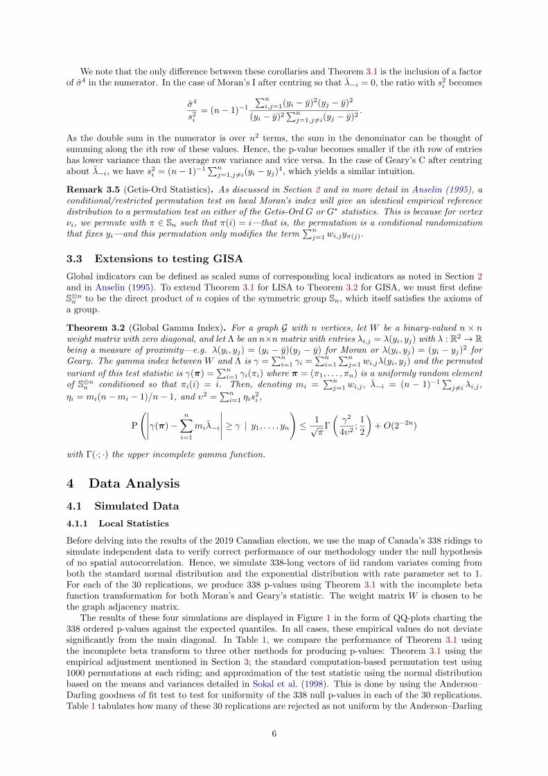
4.1.2 Global Statistics

We also test the performance of Theorem 3.2 in the null setting by simulating iid Gaussian and ex-ponential data on the entire map of Canada. Figure 2 displays the results of 400 replications of eachof the four settings. For Moran’s statistic in both cases and Geary’s statistic for Gaussian data, thedistribution of the 400 p-values is uniform as desired both visually and via the Kolmogorov-Smirnov andAnderson-Darling tests. In the case of Geary with exponential data, the p-values produced by Theo-rem 3.2 under-report the significance—i.e. the p-values are larger than they should be. This is correctedvia the following empirical beta transform detailed in Algorithm 1, which is similar to the one proposedin Kashlak et al. (2020), but modified to handle GISA statistics.

Algorithm 1 The Empirical Beta Transform for GISA Statistics

Compute p-value p0 = 1√π

Γ( γ2

4υ2 ; 12 ) based on γ chosen from the desired GISA statistic.

Choose r > 1, the number of permutations to simulate—e.g. r = 10.Draw π1, . . . ,πr from S⊗nn uniformly at random under the condition that πi,j(j) = j.

Compute r p-values by pi = 1√π

Γ(γ(πi)2

4υ2 ; 12 ) .

Find the method of moments estimator for α and β from the beta distribution.Estimate first and second central moments of the pi by p and s2,the sample mean and variance.

Estimate α = p2(1− p)/s2 − p.Estimate β = [p(1− p)/s2 − 1][1− p].

Return the adjusted p-value I(p0; α, β).

In Figure 3, we compare the statistical power of Theorem 3.2 to the classic computation-basedpermutation test. For both Moran’s and Geary’s statistic and both Gaussian and exponential data, werandomly generate 400 datasets on the map of Canada with 6 different correlation matrices being I+ciAwhere I is the identity matrix, A is the adjacency matrix for the map of Canada, and ci ranges from 0to 0.15 for Gaussian data and from 0 to 0.5 for exponential data. The permutation test was performedby simulating 500 random permutations resulting in a total of 500× 400× 6 = 1, 200, 000 permutationsin total. For Moran and Geary with Gaussian data, we see nearly identical statistical power from bothmethodologies. For Moran with Exponential data, there is a slight drop in the statistical power. In thecase of Geary’s statistic with exponential data, we lose more statistical power similar to the null settingabove. By applying the empirical adjustment from Algorithm 1, we can recover some of the lost power.As both Theorem 3.1 and 3.2 produce upper bounds the permutation test p-value, we note that thesharpness of these bounds is negatively affected when the data is heavily skewed. This is much morenoticeable in Geary’s statistic than in Moran’s statistic.

Lastly, we note that Theorem 3.2 is specifically formulated to be a two-sided test. Hence, in Figure 3,we are comparing its performance with a two-sided permutation test. As we only considered positivecorrelations in this simulation, we could have achieved higher statistical power with a one-sided test.

7

0.0 0.2 0.4 0.6 0.8 1.0

0.0

0.2

0.4

0.6

0.8

1.0

Moran with Gaussian Data

Theoretical Quantiles

Em

piric

al Q

uant

iles

0.0 0.2 0.4 0.6 0.8 1.0

0.0

0.2

0.4

0.6

0.8

1.0

Geary with Gaussian Data

Theoretical Quantiles

Em

piric

al Q

uant

iles

0.0 0.2 0.4 0.6 0.8 1.0

0.0

0.2

0.4

0.6

0.8

1.0

Moran with Exponential Data

Theoretical Quantiles

Em

piric

al Q

uant

iles

0.0 0.2 0.4 0.6 0.8 1.0

0.0

0.2

0.4

0.6

0.8

1.0

Geary with Exponential Data

Theoretical Quantiles

Em

piric

al Q

uant

iles

Figure 1: These plots depict 30 replicates of ordered p-values for Moran’s and Geary’s statistic and forindependent Gaussian and exponential data simulated on the entire map of Canada’s 338 ridings. Thisindicates that Theorem 3.1 produces p-values as would be expected in the null setting of independence.

8

0.0 0.2 0.4 0.6 0.8 1.0

0.0

0.2

0.4

0.6

0.8

1.0

Moran with Gaussian Data

Theoretical Quantiles

Em

piric

ial Q

uant

iles

KS Test: 0.769

AD Test: 0.592

0.0 0.2 0.4 0.6 0.8 1.0

0.0

0.2

0.4

0.6

0.8

1.0

Geary with Gaussian Data

Theoretical Quantiles

Em

piric

ial Q

uant

iles

KS Test: 0.433

AD Test: 0.47

0.0 0.2 0.4 0.6 0.8 1.0

0.0

0.2

0.4

0.6

0.8

1.0

Moran with Exponential Data

Theoretical Quantiles

Em

piric

ial Q

uant

iles

KS Test: 0.181

AD Test: 0.215

0.0 0.2 0.4 0.6 0.8 1.0

0.0

0.2

0.4

0.6

0.8

1.0

Geary with Exponential Data

Theoretical Quantiles

Em

piric

ial Q

uant

iles

KS Test: 0

AD Test: 0

KS Test: 0.29

AD Test: 0.087

Figure 2: These plots depict of 400 p-values of ordered p-values for global Moran’s and Geary’s statis-tic and for independent Gaussian and exponential data simulated on the entire map of Canada’s 338ridings. This indicates that Theorem 3.2 produces p-values as would be expected in the null settingof independence expect in the case of Geary’s statistic with exponential data where the blue trianglesindicate empirically adjusted p-values.

9

0.00 0.05 0.10 0.15

0.2

0.4

0.6

0.8

1.0

Global Moran with Gaussian Data

correlation

perc

enta

ge r

ejec

ted

Permutation TestAnalytic Test

0.0 0.1 0.2 0.3 0.4 0.5

0.2

0.4

0.6

0.8

Global Moran with Exponential Data

correlation

perc

enta

ge r

ejec

ted

Permutation TestAnalytic Test

0.0 0.1 0.2 0.3 0.4 0.5

0.2

0.4

0.6

0.8

Global Moran with Exponential Data

correlation

perc

enta

ge r

ejec

ted

Permutation TestAnalytic Test

0.0 0.1 0.2 0.3 0.4 0.5

0.0

0.1

0.2

0.3

0.4

0.5

0.6

0.7

Global Geary with Exponential Data

correlation

perc

enta

ge r

ejec

ted

Permutation TestAnalytic TestEmp Adjusted

Figure 3: These plots compare the statistical power of our method (blue 4) to the classic permutationtest (black ) with 500 permutations replicated 400 times at each of 6 different correlations. The firstthree cases show that equivalent power is achieved in both methodologies. For Geary’s statistic withskewed exponential data, the empirical adjustment is applied (red +’s) as in Figure 2 to recover lostpower.

10

0

2

4

6

8

30 40 50 60 70 80 90Percentage of the Popular Vote

Num

ber o

f Rid

ings

Alberta Conservatives' 2019 Election Performance

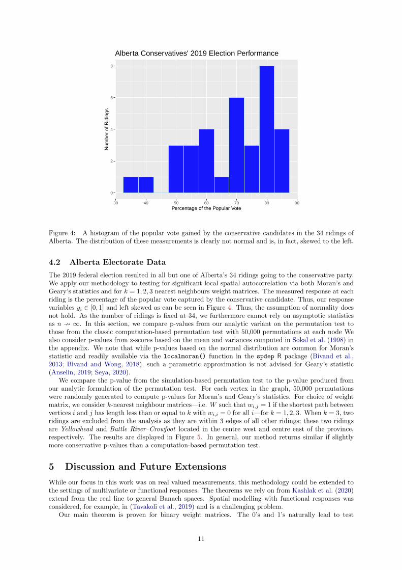
Figure 4: A histogram of the popular vote gained by the conservative candidates in the 34 ridings ofAlberta. The distribution of these measurements is clearly not normal and is, in fact, skewed to the left.

4.2 Alberta Electorate Data

The 2019 federal election resulted in all but one of Alberta’s 34 ridings going to the conservative party.We apply our methodology to testing for significant local spatial autocorrelation via both Moran’s andGeary’s statistics and for k = 1, 2, 3 nearest neighbours weight matrices. The measured response at eachriding is the percentage of the popular vote captured by the conservative candidate. Thus, our responsevariables yi ∈ [0, 1] and left skewed as can be seen in Figure 4. Thus, the assumption of normality doesnot hold. As the number of ridings is fixed at 34, we furthermore cannot rely on asymptotic statisticsas n 9 ∞. In this section, we compare p-values from our analytic variant on the permutation test tothose from the classic computation-based permutation test with 50,000 permutations at each node Wealso consider p-values from z-scores based on the mean and variances computed in Sokal et al. (1998) inthe appendix. We note that while p-values based on the normal distribution are common for Moran’sstatistic and readily available via the localmoran() function in the spdep R package (Bivand et al.,2013; Bivand and Wong, 2018), such a parametric approximation is not advised for Geary’s statistic(Anselin, 2019; Seya, 2020).

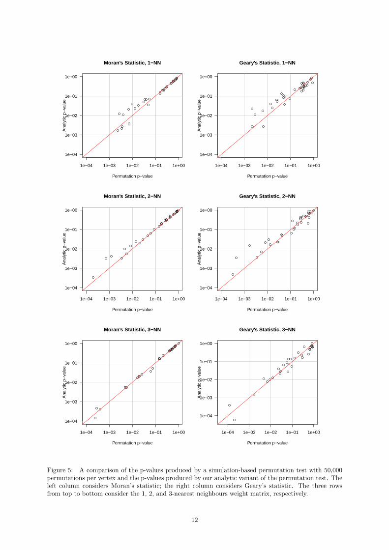
We compare the p-value from the simulation-based permutation test to the p-value produced fromour analytic formulation of the permutation test. For each vertex in the graph, 50,000 permutationswere randomly generated to compute p-values for Moran’s and Geary’s statistics. For choice of weightmatrix, we consider k-nearest neighbour matrices—i.e. W such that wi,j = 1 if the shortest path betweenvertices i and j has length less than or equal to k with wi,i = 0 for all i—for k = 1, 2, 3. When k = 3, tworidings are excluded from the analysis as they are within 3 edges of all other ridings; these two ridingsare Yellowhead and Battle River–Crowfoot located in the centre west and centre east of the province,respectively. The results are displayed in Figure 5. In general, our method returns similar if slightlymore conservative p-values than a computation-based permutation test.

5 Discussion and Future Extensions

While our focus in this work was on real valued measurements, this methodology could be extended tothe settings of multivariate or functional responses. The theorems we rely on from Kashlak et al. (2020)extend from the real line to general Banach spaces. Spatial modelling with functional responses wasconsidered, for example, in (Tavakoli et al., 2019) and is a challenging problem.

Our main theorem is proven for binary weight matrices. The 0’s and 1’s naturally lead to test

11

1e−04 1e−03 1e−02 1e−01 1e+00

1e−04

1e−03

1e−02

1e−01

1e+00

Moran's Statistic, 1−NN

Permutation p−value

Ana

lytic

p−

valu

e

1e−04 1e−03 1e−02 1e−01 1e+00

1e−04

1e−03

1e−02

1e−01

1e+00

Geary's Statistic, 1−NN

Permutation p−value

Ana

lytic

p−

valu

e

1e−04 1e−03 1e−02 1e−01 1e+00

1e−04

1e−03

1e−02

1e−01

1e+00

Moran's Statistic, 2−NN

Permutation p−value

Ana

lytic

p−

valu

e

1e−04 1e−03 1e−02 1e−01 1e+00

1e−04

1e−03

1e−02

1e−01

1e+00

Geary's Statistic, 2−NN

Permutation p−value

Ana

lytic

p−

valu

e

1e−04 1e−03 1e−02 1e−01 1e+00

1e−04

1e−03

1e−02

1e−01

1e+00

Moran's Statistic, 3−NN

Permutation p−value

Ana

lytic

p−

valu

e

1e−04 1e−03 1e−02 1e−01 1e+00

1e−04

1e−03

1e−02

1e−01

1e+00

Geary's Statistic, 3−NN

Permutation p−value

Ana

lytic

p−

valu

e

Figure 5: A comparison of the p-values produced by a simulation-based permutation test with 50,000permutations per vertex and the p-values produced by our analytic variant of the permutation test. Theleft column considers Moran’s statistic; the right column considers Geary’s statistic. The three rowsfrom top to bottom consider the 1, 2, and 3-nearest neighbours weight matrix, respectively.

12

One-Nearest-Neighbours

AlbertaM

oran

Edmonton CalgaryG

eary

Two-Nearest-Neighbours

Alberta

Mor

an

Edmonton Calgary

Gea

ry

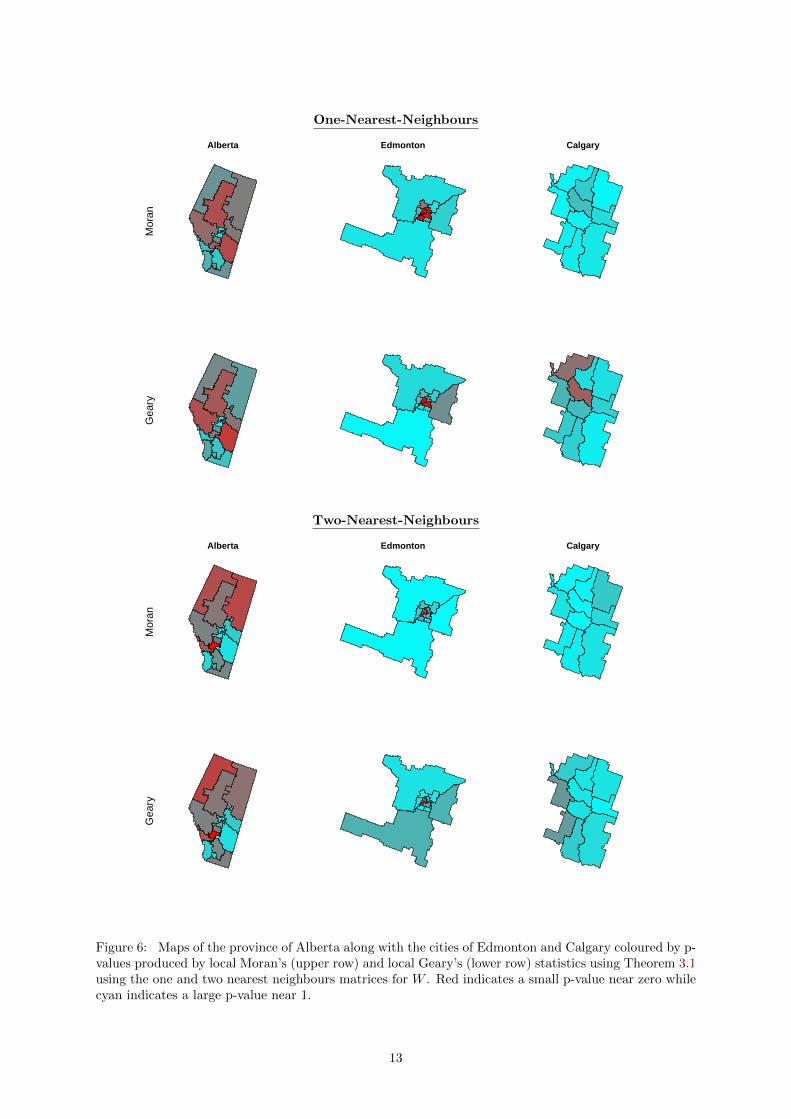
Figure 6: Maps of the province of Alberta along with the cities of Edmonton and Calgary coloured by p-values produced by local Moran’s (upper row) and local Geary’s (lower row) statistics using Theorem 3.1using the one and two nearest neighbours matrices for W . Red indicates a small p-value near zero whilecyan indicates a large p-value near 1.

13

statistics being reformulated into two sample tests so that the ideas of Kashlak et al. (2020) can beapplied. However, non-binary weight matrices are often of interest in spatial data analysis. Extensionsto such will require the adaptation of novel versions of the Khintchine inequality such as Havrilla andTkocz (2019).

Acknowledgements

The authors would like to thank the Natural Sciences and Engineering Research Council of Canada(NSERC) for the funding provided via their Discovery Grant program.

References

Milton Abramowitz and Irene A Stegun. Handbook of mathematical functions with formulas, graphs,and mathematical tables, 1972.

Luc Anselin. Local indicators of spatial association—lisa. Geographical analysis, 27(2):93–115, 1995.

Luc Anselin. A local indicator of multivariate spatial association: extending geary’s c. GeographicalAnalysis, 51(2):133–150, 2019.

Roger S Bivand and David WS Wong. Comparing implementations of global and local indicators ofspatial association. Test, 27(3):716–748, 2018.

Roger S. Bivand, Edzer Pebesma, and Virgilio Gomez-Rubio. Applied spatial data analysis with R,Second edition. Springer, NY, 2013. URL http://www.asdar-book.org/.

Andrew David Cliff and J Keith Ord. Spatial processes: models & applications. Taylor & Francis, 1981.

DLMF. NIST Digital Library of Mathematical Functions. http://dlmf.nist.gov/, Release 1.0.28 of 2020-09-15, 2020. URL http://dlmf.nist.gov/. F. W. J. Olver, A. B. Olde Daalhuis, D. W. Lozier, B. I.Schneider, R. F. Boisvert, C. W. Clark, B. R. Miller, B. V. Saunders, H. S. Cohl, and M. A. McClain,eds.

B Doman. An asymptotic expansion for the incomplete beta function. Mathematics of computation, 65(215):1283–1288, 1996.

Carlo Gaetan and Xavier Guyon. Spatial statistics and modeling, volume 90. Springer, 2010.

David JH Garling. Inequalities: a journey into linear analysis. Cambridge University Press, 2007.

Arthur Getis and J Keith Ord. The analysis of spatial association by use of distance statistics. InPerspectives on spatial data analysis, pages 127–145. Springer, 2010.

Uffe Haagerup. The best constants in the Khintchine inequality. Studia Mathematica, 70:231–283, 1981.

Alex Havrilla and Tomasz Tkocz. Sharp khinchin-type inequalities for symmetric discrete uniform ran-dom variables. arXiv preprint arXiv:1912.13345, 2019.

Orli Herscovici and Susanna Spektor. The best constant in the Khinchine inequality for slightly dependentrandom variables. arXiv preprint arXiv:1806.03562, 2020.

Lawrence J Hubert. Combinatorial data analysis: association and partial association. Psychometrika,50(4):449–467, 1985.

Adam B Kashlak, Sergii Myroshnychenko, and Susanna Spektor. Analytic permutation testing viaKahane–Khintchine inequalities. arXiv preprint arXiv:2001.01130, 2020.

Nathan Mantel. The detection of disease clustering and a generalized regression approach. Cancerresearch, 27(2 Part 1):209–220, 1967.

Hajime Seya. Global and local indicators of spatial associations. In Spatial Analysis Using Big Data,pages 33–56. Elsevier, 2020.

14

Robert R Sokal, Neal L Oden, and Barbara A Thomson. Local spatial autocorrelation in a biologicalmodel. Geographical Analysis, 30(4):331–354, 1998.

Susanna Spektor. Restricted Khinchine inequality. Canadian Mathematical Bulletin, 59(1):204–210,2016.

Shahin Tavakoli, Davide Pigoli, John AD Aston, and John S Coleman. A spatial modeling approach forlinguistic object data: Analyzing dialect sound variations across great britain. Journal of the AmericanStatistical Association, 114(527):1081–1096, 2019.

Lance A Waller and Carol A Gotway. Applied spatial statistics for public health data, volume 368. JohnWiley & Sons, 2004.

A Proofs

A.1 LISA Proofs

Proof of Theorem 3.1. We first recall that n is the total number of vertices in the graph G and that mi

is the number of edges at vertex νi. For binary weights wi,j ∈ 0, 1, we apply an affine transformationto define imbalanced Rademacher weights

δi,j =n− 1

mi(n−mi − 1)wi,j −

1

n−mi − 1∈− 1

n−mi − 1,

1

mi

for i 6= j while maintaining that δi,i = wi,i = 0. Note that since

∑j wi,j = mi that

∑j δi,j = 0.

Considering γi =∑nj=1 wi,jλi,j , we have that

γi =

n∑j=1

wi,jλi,j =mi(n−mi − 1)

n− 1

n∑j=1

δi,j + (n−mi − 1)−1

λi,j

=mi(n−mi − 1)

n− 1

n∑j=1

δi,jλi,j +miλ−i

where λ−i = (n − 1)−1∑j 6=i λi,j . Therefore, our statistic γi is equivalent up to affine transformation

to a two sample test for equality of the mean of the λi,j such that wi,j = 1 and the mean of those λi,jwith wi,j = 0 excluding the value λi,i from this test. Thus, for π being a uniformly random element ofSn, the symmetric group on n elements, with the restriction that π(i) = i, we define the permuted test

statistic to be γi(π) = mi(n−mi−1)n−1

∑nj=1 δi,jλi,π(j) + miλ−i. We note that a permutation test on γi is

equivalent to a permutation test on Ti =∑nj=1 δi,jλi,j . Let Ωi = [δ ∈ − 1

n−mi−1 , 0,1min | δi = 0, δj 6=

0 for j 6= i,∑nj=1 δj = 0] be the set of possible n-dimensional weight vectors δ that fix δi = 0. We note

the following correspondence similar to Spektor (2016) that

π ∈ Sn|π(i) = i ↔ [δ ∈ Ωi |

δi = 0 and

for i ≤ mi, δj = 1

miif π(j) ≤ mi + 1 and δj = − 1

n−mi−1 if π(j) > mi + 1

for i > mi, δj = 1mi

if π(j) ≤ mi and δj = − 1n−mi−1 if π(j) > mi

].

Thus, we can consider the permuted test statistic with respect to a dependent vector of random weightsδ ∈ Ω. That is, conditional of the yi, Ti(π) can be treated as a weakly dependent weighted Rademachersum. Applying Theorem 2.1 of Kashlak et al. (2020) for imbalanced two sample tests for equality ofmeans under Condition 3.1 that mi ≤ n−mi − 1, we have that

P (|Ti(π)| ≥ t) ≤ exp

(− m3

i t2

2s2i (n− 1)2

)where s2

i = (n− 1)−1∑j 6=i(λi,j − λ−i)2 is the sample variance of the λi,j for j 6= i. Translating back to

the local gamma index, we have

P(|γi(π)−miλ−i| ≥ γi

)≤ exp

(− m3

i

2s2i (n− 1)2

[n− 1

mi(n−mi − 1)γi

]2)

≤ exp

(− miγ

2i

2s2i (n−mi − 1)2

)

15

For the final part of Theorem 3.1, we apply the beta transform from Kashlak et al. (2020) Proposi-tion 2.5 resulting in

P(|γi(π)−miλ−i| ≥ γi

)≤ C0I

[exp

(− miγ

2i

2s2i (n−mi − 1)2

);

(n− 1)(n−mi − 1)

m2i

,1

2

]where I[·] is the regularized incomplete beta function and

C0 =

√(n− 1)(n−mi − 1)Γ

((n−1)(n−mi−1)

m2i

)miΓ

(12 + (n−1)(n−mi−1)

m2i

)with Γ(·) the gamma function.

A.2 GISA Proofs

Lemma A.1. For q > 0 and |c| < 1

2q∑k=0, kmod 2=0

Γ(q + 1)ck/2

Γ(k2 + 1)Γ(q − k2 + 1)

≥2q−1∑

k=1, kmod 2=1

Γ(q + 1)ck/2

Γ(k2 + 1)Γ(q − k2 + 1)

(A.1)

and furthermore2q−1∑

k=1, kmod 2=1

Γ(q + 1)ck/2

Γ(k2 + 1)Γ(q − k2 + 1)

= (1 + c)q +O(q−1/2).

Remark A.2. In the proof of Lemma A.1, we use a variety of transformations for hypergeometricfunctions, which can be found in the NIST Digital Library of Mathematical Functions (DLMF, 2020) aswell as in Chapter 15 of Abramowitz and Stegun (1972). These include the following where |z| ≤ 1 anda, b, c ∈ C such that R(c− a− b) > 0.

• Gauss’ summation formula, 2F1(a, b; c; 1) = Γ(c)Γ(c−a−b)Γ(c−a)Γ(c−b) for c 6= 0,−1,−2, . . . (Abramowitz and

Stegun, 1972, Eqn 15.1.20).

• Euler’s integral transform, 2F1(a, b; c; z) = Γ(c)Γ(b)Γ(c−b)

∫ 1

0tb−1(1 − t)c−b−1(1 − tz)−adt for R(c) >

R(b) > 0 (Abramowitz and Stegun, 1972, Eqn 15.3.1).

• Pfaff’s linear transform, 2F1(a, b; c; z) = (1 − z)−a2F1(a, c − b; c; zz−1 ) (Abramowitz and Stegun,

1972, Eqn 15.3.4).

• Another linear transformation 2F1(a, b; c; z) = Γ(c)Γ(b−a)Γ(b)Γ(c−a) (1 − z)−a2F1(a, c − b; a − b + 1; 1

z−1 ) +Γ(c)Γ(a−b)Γ(a)Γ(c−b) (1− z)−b2F1(b, c− a; b− a+ 1; 1

z−1 ) for |arg(1− z)| < π (Abramowitz and Stegun, 1972,

Eqn 15.3.8).

We also make use of Gautschi’s inequality for the ratio of two Gamma functions, x1−s < Γ(x+1)Γ(x+s) <

(x+ 1)1−s for s ∈ (0, 1) (DLMF, 2020, Eqn. 5.6.4).

Proof. We first note that the lefthand side of Equation A.1 is just (1 + c)q, which can be written as thegeneralized hypergeometric function 1F0(−q; ;−c).

For the righthand side, we rewrite it as

RHS(EqnA.1) =

q∑r=1

Γ(q + 1)cr−1/2

Γ(r + 12 )Γ(q − r + 3

2 )=

Γ(q + 1)√c

q∑r=1

cr

Γ(r + 12 )Γ(q − r + 3

2 )

and note that the ratio of consecutive terms is[cr+1

Γ(r + 32 )Γ(q − r + 1

2 )

] [Γ(r + 1

2 )Γ(q − r + 32 )

cr

]=

(q + 1

2 − r12 + r

)c.

16

After rescaling, we have the first q terms of the Gaussian hypergeometric function 2F1(−q − 12 , 1; 1

2 ;−c)by noting that

2F1

(−q − 1

2, 1;

1

2;−c

)= 1 +

q∑r=1

√πΓ(q + 3

2 )cr

Γ(r + 12 )Γ(q − r + 3

2 )+∑r>q

(−q − 12 )r

( 12 )r

(−c)r

= 1 +

q∑r=1

√πΓ(q + 3

2 )cr

Γ(r + 12 )Γ(q − r + 3

2 )+ cq+1

2F1

(1

2, 1; q +

1

2;−c

)where (n)r = n(n + 1) . . . (n + r − 1) is the Pochhammer symbol or rising factorial. Rearranging theabove terms gives

Γ(q + 1)√c

q∑r=1

cr

Γ(r + 12 )Γ(q − r + 3

2 )

=Γ(q + 1)

√cπΓ(q + 3

2 )

2F1

(−q − 1

2, 1;

1

2;−c

)− cq+1

2F1

(1

2, 1; q +

1

2;−c

)− 1

(A.2)

For the first hypergeometric function in Equation A.2, we apply a linear transformation formula(Abramowitz and Stegun, 1972, Eqn 15.3.8), upper bounding the second term below by setting 1/(1 + c)to 1, and then using Gauss’ summation formula to get

2F1

(−q − 1

2, 1;

1

2;−c

)= (1 + c)q−1/2 Γ( 1

2 )Γ(q + 32 )

Γ(1)Γ(q + 1)2F1

(−q − 1

2,−1

2;−q − 1

2;

1

1 + c

)+ (1 + c)−1 Γ( 1

2 )Γ(−q − 32 )

Γ(−q − 12 )Γ(− 1

2 )2F1

(1, q + 1; q +

5

2;

1

1 + c

)≤ (1 + c)q−1/2

√πΓ(q + 3

2 )

Γ(q + 1)1F0

(−1

2;

1

1 + c

)+

2F1(1, q + 1; q + 52 ; 1)

2(1 + c)(q + 32 )

= (1 + c)q−1/2

√πΓ(q + 3

2 )

Γ(q + 1)

√1− 1

1 + c+

Γ(q+ 52 )Γ( 1

2 )

Γ(q+ 32 )Γ( 3

2 )

2(1 + c)(q + 32 )

= (1 + c)q√cπΓ(q + 3

2 )

Γ(q + 1)+

1

1 + c.

For the second hypergeometric function in Equation A.2, we apply the Pfaff transform and thenEuler’s integral transform to get

2F1

(1

2, 1; q +

1

2;−c

)= (1 + c)−1/2

2F1

(1

2, q − 1

2; q +

1

2;

c

c+ 1

)= (1 + c)−1/2 Γ(q + 1

2 )

Γ(q − 12 )

∫ 1

0

tq−3/2

(1− ct

c+ 1

)−1/2

dt

≤ (1 + c)−1/2 Γ(q + 12 )

Γ(q − 12 )

∫ 1

0

tq−3/2dt

(1− c

c+ 1

)−1/2

= 1.

Putting the above bounds into Equation A.2 and upper bounding with Gautschi’s inequality we getthe desired result:

q∑r=1

Γ(q + 1)cr−1/2

Γ(r + 12 )Γ(q − r + 3

2 )≤ Γ(q + 1)√cπΓ(q + 3

2 )

(1 + c)q

√cπΓ(q + 3

2 )

Γ(q + 1)+

1

1 + c− cq+1 − 1

= (1 + c)q − Γ(q + 1)

√cπΓ(q + 3

2 )

c

1 + c+ cq+1

≤ (1 + c)q −

√q + 1

q + 12

1√π

√c

1 + c+ cq+1/2

≤ (1 + c)q − 3√2π

√1

q + 12

+1/2

(q + 12 )2

.

17

Lemma A.3. For p, n ≥ 1, let c1, . . . , cn ∈ R+. Then,∑k1+...+kn=2p

Γ(p+ 1)

Γ(k1/2 + 1) . . .Γ(kn/2 + 1)

n∏i=1

cki/2i ≤ 2n−1(c1 + . . .+ cn)p

where the sum is taken over all integer compositions of 2p.

Proof. We let ∆n2p denote the discrete simplex

∆n2p = (k1, . . . , kn) ∈ Nn | ki ≥ 0 ∀i and k1 + . . .+ kn = 2p

being the set of all n-long integer compositions of 2p ∈ N. As 2p is an even integer, we can consider evencompositions (k1, . . . , kn) such that

∑ni=1 ki = 2p and ki mod 2 = 0 for all i = 1, . . . , n, and we denote

ki = 2li. From the multinomial theorem, summing over only even compositions of 2p gives∑2l1+...+2ln=2p

Γ(p+ 1)

Γ(l1 + 1) . . .Γ(ln + 1)

n∏i=1

clii = (c1 + . . .+ cn)p.

The collection of even compositions (2l1, . . . , 2ln) forms a discrete subsimplex of ∆n2p isomorphic to ∆n

p .

We further decompose the remaining not-strictly-even (NSE) compositions of 2p into∑n/2m=1

(n

2m

)=

2n−1 − 1, disjoint subsimplices by indicating which entries in the composition are even and which areodd. This summation follows directly from the identity

∑nm=0(−1)m

(nm

)= 0. Because 2p is even, none of

the NSE subsplicies can have cardinality more than |∆np | =

(p+n−1n−1

). We will denote an NSE subsimplex

as ∆n2p(o) where o = 0, 2, 4, . . . is the number of odd entries in the composition. Each subsimplex with

exactly o odd entries is isomorphic to the others via translation. Hence, without loss of generality, wechoose the simplex ∆n

2p(o) to be the one with odd entries k1, . . . , ko and even entries ko+1, . . . , kn.

Noting that the subsimplex of even compositions is ∆n2p(0), we first prove that

(c1 + . . .+ cn)p =∑

k∈∆n2p(0)

Γ(p+ 1)

Γ(k1/2 + 1) . . .Γ(kn/2 + 1)

n∏i=1

cki/2i

≥∑

k∈∆n2p(2)

Γ(p+ 1)

Γ(k1/2 + 1) . . .Γ(kn/2 + 1)

n∏i=1

cki/2i .

by summing along a “row” of ∆n2p. We recall that entries k1 and k2 are odd in ∆n

2p(2). By fixing theremaining k3, . . . , kn, denoting 2q = 2p− k3 − . . .− kn, and applying Lemma A.1, we note that

Γ(p+ 1)

Γ(k3/2 + 1) . . .Γ(kn/2 + 1)

n∏i=3

cki/2i

∑k1+k2=2q, even

ck1/21 c

k2/22

Γ(k1/2 + 1)Γ(k2/2 + 1)

≥ Γ(p+ 1)

Γ(k3/2 + 1) . . .Γ(kn/2 + 1)

n∏i=3

cki/2i

∑k1+k2=2q, odd

ck1/21 c

k2/22

Γ(k1/2 + 1)Γ(k2/2 + 1).

Applying this for every choice of k3, . . . , kn demonstrates that the multinomial sum over all elements in∆n

2p(0) is greater or equal to the sum over all elements in any of the ∆n2p(2).

Repeating this argument shows that the multinomial sum over ∆n2p(o) is greater than or equal to the

sum over ∆n2p(o+ 2). Denoting ζ = ∆n

2p(2l) : l = 1, . . . , bn/2c to be the set of all subsimplices of ∆n2p,

we conclude that

∑k1+...+kn=2p

Γ(p+ 1)

Γ(k1/2 + 1) . . .Γ(kn/2 + 1)

n∏i=1

cki/2i

=∑∆∈ζ

∑k∈∆

Γ(p+ 1)

Γ(k1/2 + 1) . . .Γ(kn/2 + 1)

n∏i=1

cki/2i

≤ |ζ|(c1 + . . .+ cn)p ≤ 2n−1(c1 + . . .+ cn)p

by noting that |ζ| =∑bn/2cl=0

(n2l

)= 2n−1.

18

Proof of Theorem 3.2. Beginning from the proof of Theorem 3.1, we recall that we can apply an affine

transformation to write γi(πi) = mi(n−mi−1)n−1

∑nj=1 δi,jλi,πi(j) +miλ−i. Thus, our global test statistic can

be written as

γ(π) =

n∑i=1

mi(n−mi − 1)

n− 1

n∑j=1

δi,jλi,πi(j)

+

n∑i=1

miλ−i.

Inference based on the permutation test will not be affected by the constant shift term∑ni=1miλ−i.

Hence, we can proceed by considering T (π) =∑ni=1 ηiTi(πi) for η = [mi(n − mi − 1)/(n − 1)] and

Ti =∑nj=1 δi,jλi,πi(j).

We recall that π = (π1, . . . , πn) is such that πi and πj are independent random permutations fori 6= j. Then, we bound the pth moment of T (π) as follows:

ET (π)p =∑

k1+...+kn=p

(p

k1, . . . , kn

) n∏i=1

ηkii E[Ti(πi)

ki]

≤∑

k1+...+kn=p

(p

k1, . . . , kn

) n∏i=1

ηkiiki!(n− 1)kiskii

2ki/2m3ki/2i Γ(ki2 + 1)

=(n− 1)p

2p/2

∑k1+...+kn=p

Γ(p+ 1)

Γ(k12 + 1) . . .Γ(kn2 + 1)

n∏i=1

(η2i s

2i

m3i

)ki/2

=

(n− 1

21/2

)pΓ(p+ 1)

Γ(p2 + 1)

∑k1+...+kn=p

Γ(p2 + 1)

Γ(k12 + 1) . . .Γ(kn2 + 1)

n∏i=1

(η2i s

2i

m3i

)ki/2

≤(n− 1

21/2

)pΓ(p+ 1)

Γ(p2 + 1)2n−1

(n∑i=1

η2i s

2i

m3i

)p/2where the first inequality comes from Theorem A.4 of (Kashlak et al., 2020) and the second inequalitycomes from Lemma A.3 above. Symmetrizing the statistic T with π′ is an iid copy of π and applicationof Markov/Chernoff’s inequality gives

P (|T (π)| > t) ≤ infλ>0

e−λtEeλ(T (π)−T (π′))

≤ infλ>0

e−λt

[1 +

∞∑p=1

λp

p!E(T (π)− T (π′))p

]

≤ infλ>0

e−λt

[1 +

∞∑p=1

λ2p22p

(2p)!ET (π)2p

]

≤ infλ>0

e−λt

[1 +

∞∑p=1

λ2p22p

(2p)!

(n− 1

21/2

)2p(2p)!

p!2n−1

(n∑i=1

η2i s

2i

m3i

)p]

≤ infλ>0

e−λt

[1 +

∞∑p=1

2n−1

p!

2(n− 1)2λ2

p( n∑i=1

η2i s

2i

m3i

)p]

≤ infλ>0

e−λt

[1 +

∞∑p=1

(2nλ2)p

p!

(n∑i=1

(n−mi − 1)2s2i

mi

)p]

≤ infλ>0

e−λt exp

(2nλ2

) n∑i=1

(n−mi − 1)2s2i

mi

≤ exp

− t2

2n+2

(n∑i=1

(n−mi − 1)2s2i

mi

)−1 = exp

− t2

2n+2$2

where $2 =∑ni=1

(n−mi−1)2s2imi

acts like a variance for this sub-Gaussian bound.Lastly, we modify the proof of Proposition 2.5 of Kashlak et al. (2020) to improve that bound. We

19

first note that Var (Ti(π)) = s2i (

1n−mi−1 + 1

mi). Recalling the defining of ηi, we get that

Var (T (π)) =

n∑i=1

s2i η

2i

(1

n−mi − 1+

1

mi

)

=

n∑i=1

s2i

(mi(n−mi − 1)2 +m2

i (n−mi − 1)

(n− 1)2

)=

n∑i=1

ηis2i := υ2.

Thus, we apply the proof of Proposition 2.5 of Kashlak et al. (2020) to get

P

(e−

T (π)2

2n+2$2 < u

)≤ C0I

(u; 2n

$2

υ2,

1

2

)(A.3)

where I is the regularized incomplete beta function and

C0 =

(2n$

2

υ2

)1/2

Γ(

2n$2

υ2

)Γ(

12 + 2n$

2

υ2

) ≈ 1.

However, the presence of 2n in both the exponent and the beta parameter in Equation A.3 makes thisnumerically impossible to compute for moderate to large sample sizes n. Thus, we apply the asymptoticformula for the incomplete beta function detailed in Doman (1996) to get a numerically stable equationfor the tail probability.

In Doman (1996),

I(x; a, b) ∼ Q (−g log x; b) +Γ(a+ b)

Γ(a)Γ(b)xg∞∑k=0

Tk(b, x)/gk+1 (A.4)

where Q is the upper regularized incomplete gamma function, g = a + (b − 1)/2 and the Tk are powerseries related to the sinh() function and the Bernoulli polynomials. In our context, g = 2n$2/υ2−1/4 ≈2n$2/υ2. The first piece of Equation A.4 becomes

Q(−g log x; b) = Q

(2n$2

υ2− 1

4

T 2

2n+2$2;

1

2

)= Q

(T 2

4υ2− T 2

2n+4$2;

1

2

).

The second term of the asymptotic expansion contains a few subparts. First, we can use Stirling’sapproximation to show that for a→∞ with b fixed

Γ(a+ b)

Γ(a)Γ(b)∼ ab

Γ(b)=

2n/2$

υ√π

We also have that xg = exp(−T 2/2υ2). For the final series term, we only consider the first term (n=0)as gk+1 ∼ 2nk making the remainder negligible. The result is

∞∑k=0

Tk(b, x)

gk+1∼ T0(1/2, e−T

2/2n+2$2

)

2n$2/υ2∼ |T |

3/23n/2$3

2n$2/υ2=

υ2|T |3

25n/2$5

Combining all three pieces gives the expression

2n/2$

υ√π

e−T2/2υ2 υ2|T |3

25n/2$5=

1√π

υ|T |3

22n$4e−T

2/2υ2

Combining with the first part of the asymptotic expansion, we conclude that

P

(e−

T (π)2

2n$2 < u

)∼ Q

(T 2

4υ2;

1

2

)+

1√π

υ|T |3

22n$4e−T

2/2υ2

and finally that

P

(∣∣∣∣∣γ(π)−n∑i=1

miλ−i

∣∣∣∣∣ ≥ γ)∼ Q

(γ2

4υ2;

1

2

)+O(2−2n)

20

B Comparison with the Gaussian Approximation

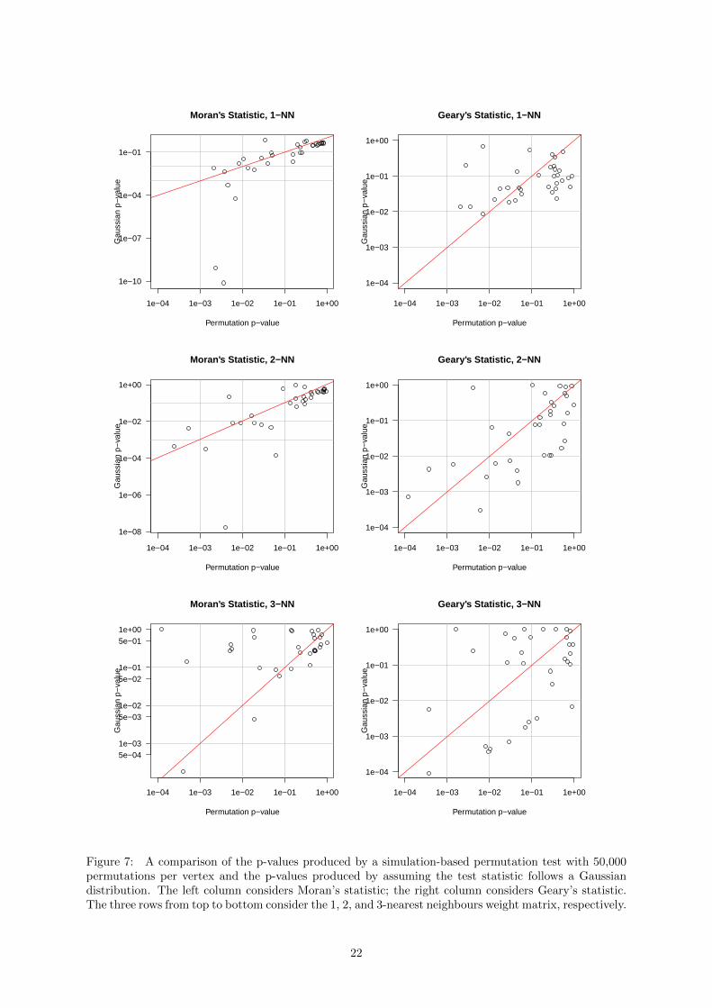
Figure 7 further reprises the analysis displayed in Figure 5 but compares the computation-based per-mutation test to the Gaussian approximation. The Gaussian approximation is not valid for the Albertaelectoral dataset as can be seen by the wild disagreement between these two methods. For Moran’sstatistic with 1-NN and 2-NN weight matrices, the Gaussian approach appears prone to overstating thesignificance of the local autocorrelation whereas for the 3-NN weight matrix, it understates the signifi-cance of many ridings. For Geary’s statistic, there is little agreement between the permutation p-valuesand the Gaussian p-values. Albeit, this departure has already been noted in Anselin (2019); Seya (2020)who recommend the permutation test for Geary’s statistic.

21

1e−04 1e−03 1e−02 1e−01 1e+00

1e−10

1e−07

1e−04

1e−01

Moran's Statistic, 1−NN

Permutation p−value

Gau

ssia

n p−

valu

e

1e−04 1e−03 1e−02 1e−01 1e+00

1e−04

1e−03

1e−02

1e−01

1e+00

Geary's Statistic, 1−NN

Permutation p−value

Gau

ssia

n p−

valu

e

1e−04 1e−03 1e−02 1e−01 1e+00

1e−08

1e−06

1e−04

1e−02

1e+00

Moran's Statistic, 2−NN

Permutation p−value

Gau

ssia

n p−

valu

e

1e−04 1e−03 1e−02 1e−01 1e+00

1e−04

1e−03

1e−02

1e−01

1e+00

Geary's Statistic, 2−NN

Permutation p−value

Gau

ssia

n p−

valu

e

1e−04 1e−03 1e−02 1e−01 1e+00

5e−041e−03

5e−031e−02

5e−021e−01

5e−011e+00

Moran's Statistic, 3−NN

Permutation p−value

Gau

ssia

n p−

valu

e

1e−04 1e−03 1e−02 1e−01 1e+00

1e−04

1e−03

1e−02

1e−01

1e+00

Geary's Statistic, 3−NN

Permutation p−value

Gau

ssia

n p−

valu

e

Figure 7: A comparison of the p-values produced by a simulation-based permutation test with 50,000permutations per vertex and the p-values produced by assuming the test statistic follows a Gaussiandistribution. The left column considers Moran’s statistic; the right column considers Geary’s statistic.The three rows from top to bottom consider the 1, 2, and 3-nearest neighbours weight matrix, respectively.

22