Computation and Applications of Industrial Leading ...users.cis.fiu.edu/~taoli/pub/05-kpiforsmcc01.pdffactoring out the key performance indicators ... methodology for KPI analysis

Abstract— Within Business Intelligence (BI) systems, an industrial Key Performance Indicator (KPI) is a measurement of how well the industrial process in the organization performs an operational activity that is critical for the current and future success of that organization [1]. The industrial leading indicators are one type of KPIs that present key drivers of industrial business value, are predictors of future outcomes. Thus leading indicator discovery is critical to success of the industrial objectives. There are some challenges in leading indicator discovery. The traditional approach depending on domain experts’ experiences is labor-intensive and error-prone. In addition, because the time shifts between industrial KPIs are vague and often inconstant for variability of business concerns, the correlation between them cannot be correctly calculated using the traditional distance functions. In this paper, we propose a semi-automatic system with an iterative learning process for discovering leading indicators to help trace anomalies and optimize the industrial objectives. Finally two industrial case studies are conducted by applying the proposed methods in the production printing application. The proposed system has two key differentiations and novelties: (1) the semi-automatic framework uses temporal data mining techniques combined with domain knowledge to enable timely access to KPI analysis, and anomaly tracing; and (2) an iterative learning method continuingly uncovers the “root” leading indicators along with the changes of business environment.

Index Terms—KPI, Leading Indicator, Business Process, Iterative

Learning, Anomaly, Time Series.

I. INTRODUCTION ithin Business Intelligence (BI) systems (e.g., business dashboard, business performance management, management information system, etc.),

industrial Key Performance Indicators (also known as KPI) are one tool used to convey the relative health of the business, or a portion of that business. A KPI is a specific metric (a quantitative, periodic measurement of one or more processes), chosen from all of the collected or possible industrial metrics within a business in such a manner as to

This work is partially supported by NSF CAREER Award IIS-0546280

and a Xerox UAC (University of Affairs Committee) award. Wei Peng, Tong Sun and Philip Rose are with the Xerox Innovation

Group, Xerox Corporation, Webster, NY 14580 USA (e-mail: {Wei.Peng, Tong.Sun, Philip.Rose}@xerox.com).

Tao Li is with the School of Computer Science, Florida International University, Miami, FL 33199 USA (e-mail: [email protected]).

convey the most amount of information in a single measurement – the “key” measurement. As such, a KPI is a quantifiable measurement of how well an operational, tactical or strategic activity is performed and progressed in the industrial process within an organization [1]. KPIs must reflect the critical success factors of an organization. Not all metrics are indicators, not all indicators are KPIs either, but all KPIs are indicators and all indicators are metrics, thus defining an ontological hierarchy of measurements.

There are three types of KPI [1]: (1) Leading indicator: “a KPI that measures activities that have a significant effect on future performance of industrial objectives” which are causal roots of the outcome (i.e. lagging indicator) they influence, and actionable for the future performance against one or more lagging indicators; (2) Lagging indicator: a KPI that measures the output of past activities; and (3) Diagnostic measure: a KPI that is neither leading nor lagging, but signals the health of industrial processes or activities. For example[1], “Number of clients that sales people meet with face to face each week” may be a leading indicator of “Sales Revenue” (a lagging indicator or outcome); “Complex repairs completed successfully during the first call or visit” be a leading indicator of “Customer Satisfaction” (a lagging indicator or outcome). “Throughput” should be a diagnostic measure of “Efficiency” of a production workflow. Leading indicators are very powerful metrics in that they possess not only the predictive and insightful causal relationship(s) within the business process(s), but also enable the actionable course for continuing industrial process improvement. Therefore, creating effective leading KPIs is critical to the success of any business organization so that not only it is agile to changes, but also is prepared for changes in advance. However, identifying leading indicators is often hard and tricky requiring months to collect requirements, standardizing definitions and rules, prioritizing metrics, and soliciting feedback, etc. Moreover, because the time shifts between the leading indicators and the corresponding

Computation and Applications of Industrial Leading Indicators to Business Process

Improvement Wei Peng, Tong Sun, Philip Rose, and Tao Li

W

INTERNATIONAL JOURNAL OF INTELLIGENT CONTROL AND SYSTEMS VOL. 13, NO. 3, SEPTEMBER 2008,196-207

Fig. 1. The Schematic View and Iterative Steps

affected lagging indicators are vague and often inconstant for variability of business concerns, the traditional approach depending on domain experts’ experiences is labor-intensive and error-prone. Given that 20% of the work in developing a successful KPI comes from a deploy-observe-adjust cycle [1] – i.e. putting a KPI into a BI system, seeing how it impacts behavior and performance, and then adjusting accordingly – many of the KPIs visible in a typical BI system at any point in time are not delivering full value to the users of these systems. Furthermore, it is much more challenging to identify the more powerful value-driver KPIs (i.e. leading indicators). Finally, many traditional BI systems, such as Business Scorecard [12], Executive Information Systems [13], Dashboard [14,15], deliver primarily pre-defined historic metrics (or lagging indicators) for a long-term strategic or mid-term tactical analysis, and lack the necessary flexibility to support evolving metrics or data collection points over time for real-time operational analysis. There are also some BI systems improving business process quality through managing exceptions or execution quality [16,17].

In this paper, we propose a semi-automatic system with an iterative learning process for analyzing operational metrics, factoring out the key performance indicators (KPIs) and then further discovering leading indicators by applying certain data mining techniques incorporated with the domain knowledge. The system involves domain experts to define the KPIs and validate the leading indicators to avoid “black-box” effects [20]. In order to illustrate how the proposed system and methods can be applied in a specific business process, two case studies have been conducted for typical real-world production print workflows (e.g.,

transaction printing, and book printing, as examples). The major challenges being investigated and addressed in this paper are:

• How to automate the computation intensive data analysis while incorporating as much domain knowledge as possible?

• How to effectively factor out overlapping or non-critical metrics?

• How to calculate the approximate influencing time shifts between correlated metrics?

• How to measure the significance of causal relationships between the leading indicators and the metrics they predict?

• How to enable the addition of new data collection points if the resulting leading indicators are not satisfactory based on domain knowledge, when business concerns change, or when other alternations occur within the underlying organization?

Compared with the traditional analytic capabilities in most existing BI systems, the proposed system and methods have two key differentiations and innovations: (1) the semi-automatic framework simplifies many traditional labor-intensive and error-prone steps through the application of temporal data mining techniques (e.g., dynamic time warping, Granger Causality, adaptive agglomerative clustering) combined with specific domain knowledge, thus enabling timely access to operational metrics, KPI analysis, and powerful leading indicator discovery; and (2) an iterative learning methodology not only continuingly uncovers the “root” leading indicators,

INTERNATIONAL JOURNAL OF INTELLIGENT CONTROL AND SYSTEMS, VOL. 13, NO. 3, SEPTEMBER 2008 197

but also enables the flexibility and adaptability for metrics updates and additional data collection points.

The discovered leading relationship also helps to correlate the detected anomalies in business processes. Anomalies indicate some unexpected situations such as operational or business measurement below a certain threshold [23,24]. As we know, anomaly detection and tracing are critical to keep a business process workflow running soundly. Even small faults may cause the whole workflow process unable to work properly. However detecting, understanding, and tracing anomalies in the complex business process are not trivial since the states of business workflow components vary along time, anomalies usually propagate, and the number of anomalies is too small. We propose to trace anomalies and identify the anomaly sources by looking for the correlation between the KPIs where the anomalies present instead of looking for the correlation between the anomalies directly.

The rest of our paper is organized as follows: Section II describes the system scheme and the iterative learning methodology for KPI analysis and leading indicator discovery. Section III introduces Dynamic Time Warping (DTW) and Granger Causality in leading indicator identification. Section IV specifies how to use adaptive agglomerative clustering to construct causal relation hierarchy between KPIs, and find the critical root leading indicators. Section V presents how to detect anomalies and trace them in a business process by using leading indicator discovery techniques. Two case studies that are based on the discrete event simulations of the real-world production printing workflows are illustrated in Section VI. Section VII concludes the paper with summary and future research topics. The preliminary version of this paper is published in [19].

II. SYSTEM SCHEME FOR KPI ANALYSIS LEADING INDICATOR DISCOVERY

Figure 1 illustrates the schematic view of various elements and steps within the proposed system and iterative learning process for KPI analysis and leading indicator discovery. It consists of the following 10 major steps (numbered from 1 to 10 in Figure 1): 1. For any business organization, the underlying domain

model, which encapsulates business goal, business process and workflow model, key terminology and relationships, business assumption, etc., drives the definition of data collection points (or data model) that need to be tracked in a BI system. The Raw Data is the basic data entities, which may be culled from recorded events, workflow or machine logs, metrics, etc., and provides a baseline data source for further data-driven analysis.

2. Usually, the domain experts identify and define KPIs and their formulas based on existing raw data, business goals, and personal experience. Some KPIs are generic -- for example, process efficiency and throughput are generic measurements in the manufacturing domain. Some KPIs are customized to a particular business goal or application – for instance, the number of impressions achieved on a press is customized to the printing domain, but bears little meaning in other manufacturing environments. The metrics used in this step are specific sets of time series data from step 1 as identified by the domain expert.

3. In a complex system, a significant number of metrics

may be collected. Some metrics contain little information related to certain business goals, and some metrics are overlapping. It is critical to filter out the less important metrics or noises and focus on the small number of metrics in a particular business context that yield the greatest business value. We propose to use unsupervised dimensionality reduction techniques, such as Principal Component Analysis (PCA) [2]/Singular Value Decomposition (SVD) [3] to filter out the less significant metrics. In addition, an unsupervised dimensionality reduction technique, Piecewise Aggregate Approximation (PAA) [4] can help to reduce the time dimensionality of each time series if the computational efficiency is required.

4. In order to discover leading indicators, we explore the

correlations among the reduced indicator sets by considering the time-shifts [11]. Traditional metric distance functions, including Euclidean distance and correlation coefficients, are not suitable for detecting correlation between time series. Non-metric distance functions like Dynamic Time Warping (DTW), which is widely used in speech recognition, is well suited for leading indicator discovery. DTW applies dynamic programming with time composition and decomposition [5] to discover the best alignment warp with the minimum alignment distortion (distance). This alignment warping path can then be used to compute the time shifts between various metrics, to help determine the time order of these metrics, and to construct the causal hierarchy. In the case of two highly correlated metrics it is often the case that the one appearing before the other is a leading indicator to the other. However, there are two disadvantages of utilizing DTW for leading indicator discovery: (a) the highly correlated time series does not provide theoretic foundation of any causal relationships between the series themselves; and (b) it is difficult to define the threshold alignment warping distance. In order to overcome these drawbacks we next apply Granger Causality [6] in order to test causal direction between the time series.

198 Peng et al: Computation and Applications of Industrial Leading Indicators to Business Process Improvement

This determines whether one time series variable can help to predict the other. Although Granger Causality is unable to obtain the time shifts, it provides the solid statistical foundation for the leading indicator discovery and establishes the significance scores of causal relationships between metrics. Therefore, we use both DTW and Granger Causality to derive the distance matrix among indicators, which dictate the correlation between any two indicators. Detailed technical content regarding DTW and Granger Causality are provided in Section 3.

5. Any specific metric may have many leading indicators,

each of which could in turn lead to additional metrics. This many-to-many directional complexity increases polynomially as the number of indicators increases. Therefore, after the correlation distance matrix is derived in step 4, we propose the use of adaptive agglomerative clustering to obtain the hierarchical relationships in a dendrogram, thus partitioning all of the metrics into clusters. The details behind this proposed clustering algorithm are provided in Section 4.

6. All metrics falling into the same cluster at this point are

more highly correlated with each other than across the clusters. Within an individual cluster, the metrics preceding others are assumed to be the root leading indicators for this cluster.

7. After the root leading indicator is discovered from each

cluster in step 6, the domain experts will examine them against the underlying domain model and determine whether the resulting leading indicators are actionable and/or meaningfully critical in certain business context.

8. In some cases, the domain experts will discover one or

more leading indicators with actionable characteristics, thus designating these indicators as the desired leading KPI. As business processes change, the entire discovery process, from step 1 to step 7, continuingly progresses, such that the resulting leading indicators also change over time.

9. In other cases, the domain experts may decide to delete

or devalue some indicators, or decide to add more metrics (which may imply new data collection points to be added) to the domain model. As the underlying domain model is updated, the scheme of raw data collection is evolved via expansion or merging. Meanwhile, the entire discovery process, from step 1 to step 7, continuingly progresses, such that the resulting leading indicators also change over time.

10. Over time the business concerns or context will change, and the domain model is updated accordingly. Similarly, the entire discovery process, from step 1 to step 7, continuingly progresses, such that the resulting leading indicators may evolve over time.

In summary, the above 10 steps illustrate an iterative learning methodology to discover the leading indicators in a business process over time via data mining techniques combined with domain knowledge guidance. The learned leading indicators can also evolve with changing business objectives, and those that are determined to be actionable are implemented as KPIs within the environment so that continuing process improvement is enabled.

III. LEADING INDICATOR IDENTIFICATION

METHODS As we discussed in the last section (step 4 of the iterative

process), in order to discover leading indicators, we first need to compute the “time shifts” between the time series indicators, define the threshold alignment warping distance for “high correlation” between the indicators, and then determine whether there is any “causal relationship” from the “high correlative” pairs. We find that DTW and Granger Causality complement each other and serve well for the above two purposes in leading indicator discovery. This section provides detailed descriptions on how these two techniques can be used jointly in uncovering leading indicators from a set of time series indicators.

A. Using Dynamic Time Warping to Discover the Correlation and the Time Order of Indicators First, we use Z-score normalization [7] to remove the

baseline and re-scale the indicators so that the range of all indicators has mean of zero and variance of one. Then we use Dynamic Time Warping (DTW) that is often applied in speech and handwriting recognition [24] to discover the nonlinear alignment similarity between KPIs.

Suppose we have KPI X, which has the value sequence [X1, X2, … , Xn], and KPI Y , which has the value sequence [Y1, Y2, …, Ym] over time. The best warping distance DTW(X, Y) between X and Y is presented as:

(1) where D(Xn, Ym) is the local distance between the elements Xn and Ym, and X(1, n-1) and Y(1, m-1) are the subsequences [X1, X2, …, Xn-1] and [Y1, Y2, …, Ym-1] respectively. A threshold need to be set such that if the best warping distance DTW(X, Y) is below it there should exist a high correlation between X and Y.

For leading indicator discovery based on DTW, we use the alignment warp path to discover the time order in highly


correlated indicators and the approximate time shifts between them. The alignment warp path is composed of two arrays which are of the same length, each of which consists of the increasing or decreasing position numbers in an indicator. The elements of the same array number in the two arrays are matched positionally by DTW to achieve the optimal alignment. Let the alignment warp path between KPI X and KPI Y be composed of arrays PX and PY from X and Y respectively. The time shift between X and Y is abs(mode(PX - PY )), where abs is the absolute value function. Mode(x) returns the element with the highest frequency in the array x.

• If mode(PX - PY ) < 0, KPI X precedes Y , and is considered as the leading indicator of Y if X and Y are highly correlated.

• If mode(PX - PY ) > 0, Y is the leading indicator. • If mode(PX - PY ) = 0, X and Y do not exhibit a

leading relationship in either direction. For example, given X be [4, 5, 3, 6, 8] and Y be [5, 2, 7, 8, 9], the alignment warp path PX is [1, 2, 3, 4, 5, 5] and PY is [1, 1, 2, 3, 4, 5]. The time shift between them is 1, and KPI Y is preceding KPI X if they are regarded to be highly correlated.

B. Using Granger Causality to Score the Significance of Causal Relationship

Granger Causality [6] is a measure to determine whether one time series helps to predict another time series. Given lagged values of X and Y from time 1 to t-1, we want to forecast the value of Y at time t. We say that X Granger-cause Y, if the variance of the optimal linear prediction based on lagged X and Y is smaller than if only based on lagged Y. In other words, the addition of lagged X to lagged Y makes better prediction than only lagged Y. Granger Causality usually uses an F-test on the lagged values of X and Y to test whether X provides significant information of the future values of Y.

Let Yi and Xi be the values of Y and X at time i respectively. The data are described with a bivariate vector regressive model:

(2) where k is the lag length, α and β are coefficients, and єt is the error term. The null hypothesis H0 is α1 = α2 = … = αk = 0. The equation (2) restricted under the null hypothesis is the model:

. (3)

The residues Res1 and Res0 of these two models are and , where n is the whole test time. The sum of

squares of residues in these two models can be transformed to a modified ratio which is:

. (4) TS, or “test statistic” follows an F-distribution if the null hypothesis is true. The value of test statistic is assigned a significance p-value, which is in the range of [0, 1], by comparing to the corresponding entry in the table of F-test critical value. The smaller the significance score, the higher the possibility to reject the null hypothesis, or to accept the causal relationship. The significance score is directional. If the significance score of X to Y is small enough, while the significance score of Y to X is not, we regard X as the leading indication of Y, and vice versa. If the scores of two directions are very close, neither is presumed to have a leading relationship to the other.

IV. ROOT LEADING INDICATOR IDENTIFICATION METHODS

Any specific metric may have many leading indicators,

each of which could in turn lead to additional metrics. This many-to-many directional complexity increases polynomially as the number of indicators increases. Domain experts are unable to determine all of the leading indicators, and decision making is impossible when there are too many leading indicators to be optimized. Therefore complexity must be reduced to provide focus on the critical leading indicators. These critical leading indicators are called root leading indicators and are root causes of one or more key metrics. We propose the use of adaptive agglomerative clustering to obtain the hierarchical relationships in a dendrogram, thus partitioning all of the metrics into clusters and ultimately identifying the “root” leading indicators.

From the results of DTW and Granger Causality, we derive the distance matrix wherein each cell is a value indicating the correlation between the corresponding row metric (represented as Ki) and the column metric (represented as Kj), and the diagonal values are zeros. In case of DTW, the cell value is the alignment warping distance. In case of Granger Causality the significance scores are directional, thus we need a transformation to determine the distance matrix. In the Granger Causality distance matrix, the cell value of row Ki and column Kj is equal to the cell value of row Kj and column Ki, and is equal to the smaller significance score in the scores from Ki to Kj and from j to i. After the distance matrix is derived, agglomerative clustering constructs a dendrogram on top of the metrics. The metrics are then partitioned into clusters such that metrics within the same cluster have a higher correlation between each other as compared to the metrics in other clusters.


By cutting different edges in the aforementioned dendrogram we can obtain a different number of clusters. However, where to cut the edges is uncertain in the traditional agglomerative clustering, and even domain experts cannot determine the number of clusters in a complex set of metrics. Modified agglomerative clustering is able to solve this problem. The cluster number can be determined by Akaike Information Criterion (AIC) - essentially the log-likelihood of the model increasingly penalized by the number of parameters. The AIC score of a cluster assignment Ci is defined as:

(5) where L(Ci) is the log-likelihood of Ci. K × m is the number of parameters in the model. K is the number of clusters, and m is the number of coordinates of each metric. We assume that each cluster is following multivariate Gaussian distribution. The log-likelihood L(Ci) is:

, (6) where nj is the number of metrics in cluster j, and σj is estimated by the average distance between all pairs of metrics in cluster j. The cluster number that obtains the highest AIC score is chosen.

Because the metrics in the same cluster are cohesive based on the non-traditional correlation function, σj is calculated using the warping distance matrix from DTW. Moreover, we also project the metrics into the two dimensional space where the traditional distance function preserves the property of the correlation obtained from DTW in the original space. The visualization of metrics in this latent two-dimensional space helps to determine the number of clusters, and offers vivid intuitions of the relationships between metrics [22]. We use multidimensional scaling (MDS) to create a space that faithfully captures the observed correlation between entities in this space [8, 9]. In our experiment, the input n × n pairwise distance matrix of n metrics is transformed to an n × 2 matrix such that every metric is projected into a two dimensional space. In each of the obtained clusters the metrics are sequenced based on the time order and shifts between them. The metrics preceding all other metrics in the cluster are regarded as the root leading indicators of the other metrics in this cluster.

V. TRACING ANOMALIES We adopt Adaptive Threshold [18] to detect anomalies in

each KPI. It uses Exponentially Weighted Moving Average (EWMA) [21] to estimate the recent mean of the time series KPI, and adaptively sets the alarm threshold. If the KPI is below the threshold at a particular time, the alarm signals.

Given a KPI w, and the value of w at time i wi, the alarm signals when: wi < αμi-1, where μi-1 is calculated from the past history of w before time i. α in the range (0, 1) is the percentage of mean value below which the alarm prepares to signal. μi can be estimated by using EWMA as follows

, (7) where λ is the EWMA factor. The direct use of the above algorithm may yield many false alarms. Usually it is modified such that if there are a certain number of successive violations of the threshold, then the alarm signals. Before tracing anomalies in workflow, the correlations between anomalies need to be mined. Since the number of anomalies is usually too few to extract any correlation rules, we assume that highly correlated anomalies should lie in highly correlated KPIs. If anomalies show the leading relationship extracted from their KPI analysis process, the anomaly appearing first within a range of a certain time period is the anomaly source. For example, the anomaly a is detected in KPI A at time ta, the anomaly b is detected in KPI B at time tb, and if we find the KPI A is the leading indicator of KPI B with the time shift T and tb-ta is in the range (0, T+ ε), where ε is a small positive value due to time shift estimation error, then a is the anomaly source of b. If an anomaly c in KPI C is detected at time tc, C is leading B in time T’, and tc-tb is in the range (0, T’+ ε), then c is the anomaly source of a and b.

VI. CASE STUDIES In order to illustrate how the proposed system and

methods can be applied in specific business processes, and how the leading indicators help guide decision making, a study was made of two typical real-world workflows in production printing domain: transactional printing and book production. The first case study gives a detail description of applied techniques of leading indicator discovery and anomaly tracing process. The second case study mainly focuses on the iterative process. A domain-expert helped construct two discrete event driven domain models based on real world printing applications that in turn drove the data collection points (or metrics), KPI filtering, and leading indicator validation. The discrete event model tracks asynchronous discrete incidents (or events) with the system state transitions based on specified time intervals [10], thus delivering the time series data required for these case studies.

A (1) Leading Indicator Discovery in a Transactional Production Printing Workflow Scenario Figure 2 illustrates a transactional production printing

workflow model, consisting of 7 activities or operations (shown in circles) connected via transactions (shown as rectangles). Some of the activities or operations can be


performed either automatically or manually. For example, check printing is a typical transactional printing workflow, which usually involves a “shell” (a pre-printed empty check form or frame), and a variable information (VI) data stream that contains the individualized content for each check. The upstream workflow activities include designing the check shell (“Generate Shell Format”) and transaction data model for check content (“Generate Transaction VI”). Before production starts, the check shells are pre-printed (“Generate Shell”) and loaded into the printer (“Load Shell”). As soon as the production cycle kicks off, the transaction VI stream is combined with its overlay shell form and the composed result is then printed on the pre-printed and loaded checks shells at a production printer. Finally, finishing operations (such as cut and fold) take place on the printed checks. Figure 3 shows the 7 time series indicators that are the throughput metrics of each constituent activity or operation in the case study of transaction workflow model. More specifically, GenShellFormat, GenShell, LoadShell, GenVIData, VIComp, Printing, and CutFold are the throughput metrics of “Generate Shell Format”, “Generate Shell”, “Load Shell”, “Generate Transaction VI”, “VI Data Composition”, “Printing”, and “Cut & Fold”, respectively.

In this scenario, we assume that the processing time for each activity within the workflow model follows a different Gaussian distribution. The flow of one activity to the next is delayed for some specified time, and noise exists in the model according to the actual environment. Specifically, the operator needs 20 minutes to transfer items from the synchronized activities “Generate Shell Format” and “Generate VI Data” to activity “VI Data Composition”; it takes 10 and 15 minutes to transfer from the previous activities to “Printing” and from “Printing” to “Cut&Fold” respectively. There exists 5 minutes from “Generate Shell” to “Load Shell”. The indicators in Figure 3 are time series data tracking the throughput of each activity (transactions per minute) over a total recording time of 500 minutes.

The cell value in the symmetric matrix in Table 1 represents the optimal warping distance between the corresponding column metric and the corresponding row metric. Thus, the smaller the cell value, the higher possibility of the corresponding column metric highly correlated with the corresponding row metric. The significance score of metric i Granger-causing metric j is recorded in the cell intersecting row i and column j in Table 2. The smaller the significance score, the higher the causal relationship existing between the corresponding row metric and column metric. The time shift matrix in Table 3 is calculated from the alignment warp path. The positive cell value means that the row metric appears before the column metric. On the contrary, the negative cell value means the column metric appears before the row metric. Zeros in cells indicate diagnostic relationship.

Fig. 2. A transaction production printing workflow scenario

Fig. 3. Seven transaction printing time series KPIs

Fig. 4.The dendrogram of agglomerative clustering on transaction printing KPIs and visualization of KPIs From these three tables, it can be seen that GenShell is highly correlated to LoadShell. This is because the corresponding operations are directly connected in the workflow model. The time shift between them is calculated by using DTW to be 5, as shown in Table 3 that indicates GenShell leads LoadShell.


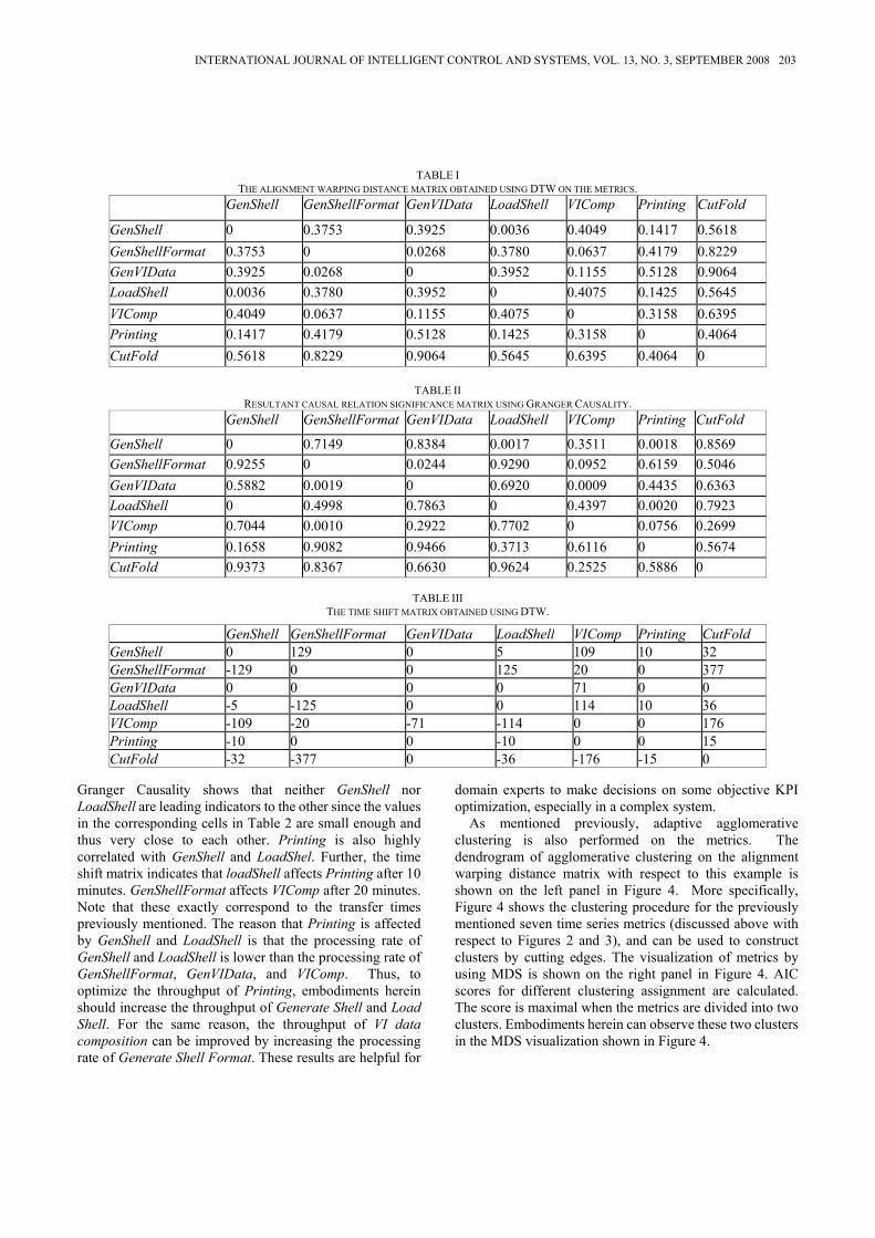
TABLE I

THE ALIGNMENT WARPING DISTANCE MATRIX OBTAINED USING DTW ON THE METRICS. GenShell GenShellFormat GenVIData LoadShell VIComp Printing CutFold

GenShell 0 0.3753 0.3925 0.0036 0.4049 0.1417 0.5618 GenShellFormat 0.3753 0 0.0268 0.3780 0.0637 0.4179 0.8229 GenVIData 0.3925 0.0268 0 0.3952 0.1155 0.5128 0.9064 LoadShell 0.0036 0.3780 0.3952 0 0.4075 0.1425 0.5645 VIComp 0.4049 0.0637 0.1155 0.4075 0 0.3158 0.6395 Printing 0.1417 0.4179 0.5128 0.1425 0.3158 0 0.4064 CutFold 0.5618 0.8229 0.9064 0.5645 0.6395 0.4064 0

TABLE II

RESULTANT CAUSAL RELATION SIGNIFICANCE MATRIX USING GRANGER CAUSALITY. GenShell GenShellFormat GenVIData LoadShell VIComp Printing CutFold

GenShell 0 0.7149 0.8384 0.0017 0.3511 0.0018 0.8569 GenShellFormat 0.9255 0 0.0244 0.9290 0.0952 0.6159 0.5046 GenVIData 0.5882 0.0019 0 0.6920 0.0009 0.4435 0.6363 LoadShell 0 0.4998 0.7863 0 0.4397 0.0020 0.7923 VIComp 0.7044 0.0010 0.2922 0.7702 0 0.0756 0.2699 Printing 0.1658 0.9082 0.9466 0.3713 0.6116 0 0.5674 CutFold 0.9373 0.8367 0.6630 0.9624 0.2525 0.5886 0

TABLE III

THE TIME SHIFT MATRIX OBTAINED USING DTW.

Granger Causality shows that neither GenShell nor LoadShell are leading indicators to the other since the values in the corresponding cells in Table 2 are small enough and thus very close to each other. Printing is also highly correlated with GenShell and LoadShel. Further, the time shift matrix indicates that loadShell affects Printing after 10 minutes. GenShellFormat affects VIComp after 20 minutes. Note that these exactly correspond to the transfer times previously mentioned. The reason that Printing is affected by GenShell and LoadShell is that the processing rate of GenShell and LoadShell is lower than the processing rate of GenShellFormat, GenVIData, and VIComp. Thus, to optimize the throughput of Printing, embodiments herein should increase the throughput of Generate Shell and Load Shell. For the same reason, the throughput of VI data composition can be improved by increasing the processing rate of Generate Shell Format. These results are helpful for

domain experts to make decisions on some objective KPI optimization, especially in a complex system.

As mentioned previously, adaptive agglomerative clustering is also performed on the metrics. The dendrogram of agglomerative clustering on the alignment warping distance matrix with respect to this example is shown on the left panel in Figure 4. More specifically, Figure 4 shows the clustering procedure for the previously mentioned seven time series metrics (discussed above with respect to Figures 2 and 3), and can be used to construct clusters by cutting edges. The visualization of metrics by using MDS is shown on the right panel in Figure 4. AIC scores for different clustering assignment are calculated. The score is maximal when the metrics are divided into two clusters. Embodiments herein can observe these two clusters in the MDS visualization shown in Figure 4.

GenShell GenShellFormat GenVIData LoadShell VIComp Printing CutFold GenShell 0 129 0 5 109 10 32 GenShellFormat -129 0 0 125 20 0 377GenVIData 0 0 0 0 71 0 0 LoadShell -5 -125 0 0 114 10 36 VIComp -109 -20 -71 -114 0 0 176 Printing -10 0 0 -10 0 0 15 CutFold -32 -377 0 -36 -176 -15 0


The metrics in the same cluster are identified similarly in Figures 2 and 4. One cluster has GenShell, LoadShell, Printing, and CutFold. The other has GenShellFormat, GenVIData, and VIComp. In the former cluster, the root leading indicator is GenShell as the results of DTW, or both GenShell and LoadShell are root leading indicators as the results of Granger Causality. In the latter cluster, the root leading indicator is GenShellFormat. If the focal lagging indicator is the finishing throughput (The finishing throughput is the throughput of the activity ‘Cut & Fold’), GenShell is its root leading indicator according to DTW. After domain experts (or users) examine the results obtained from leading indicator analysis, they could decide to increase the processing rate of the activity ‘Generate Shell’ to optimize the finishing throughput. In this example, the time that this leading indicator affects the finishing throughput is approximately 30 minutes. After improving GenShell and LoadShell, the finishing throughput is almost doubled told by domain experts.

A (2) Tracing Anomalies in the Transactional Production Printing Workflow Scenario Take this transaction beta printing workflow as an

example. Adaptive Threshold algorithm can find anomalies in three KPIs, GenShell, LoadShell, and Printing. These three KPIs from time 231 to time 280 and the alarm thresholds below which the alarm prepares to signal are illustrated in Figure 5. α and λ are set to 0.5 and 0.98 respectively. From Figure 5, we note that GenShell rings the alarm after time 242, LoadShell after time 247, and Printing after time 252. We define that until there are 3 consecutive violations of the threshold, the alarm rings. The anomalies of GenShell, LoadShell and Printing denoted as “A”, “B”, and “C” in Figure 5, occur at 245, 250, and 255 respectively. Note that Adaptive Threshold detects all anomalies without any false alarms. In order to trace the anomalies, we first find that these three anomalies are in the highly related KPIs. By observing the time shift matrix in Table III, GenShell precedes LoadShell by 5 minutes, and LoadShell precedes Printing by 10 minutes too. Obviously, the anomaly “C” occurs in operation “Printing” can be traced back to operation “Load Shell”, and then to operation “Generate Shell”. Thus the operators can go to the operation “Generate Shell” directly to solve the problem in the original anomaly source instead of inspecting all three operations.

B A Book Printing Workflow Scenario Figures 6-8 demonstrate an example of an evolving

procedure of leading indicator analysis for an example book printing workflow scenario. Figures 6-8 illustrate a book printing workflow model along the top of each figure, with a dendrogram of the agglomerative clustering on the alignment warping distance matrix shown to the left below each printing workflow model, and a visualization of metrics by using MDS shown to the right below each

printing workflow model. In this case study, the tested dataset contains three evolving phases of book printing. More specifically, Figures 6, 7, and 8 illustrate the evolving process of leading indicator analysis and how it guides the decision making for continuing process improvement.

Fig. 5. Three KPIs from the transaction printing workflow, alarm threshold, and anomalies.

In this example, the book printing workflow involves book submission, printer setup, printing, folder setup, folding, staple setup, and stapling. Folder setup and staple setup are assumed to be required for all books. However, printer setup is only necessary when the book type (e.g., perfect bound book, booklet, case bound book, etc.) has changed from a previous book to the current book. If both the previous book and current book have the same paper type, the same color requirement, etc., the printer does not need to be set up. Otherwise, certain amount of time is consumed for printer setup. The processing time for all the activities (or operations) depends on the volumes of books and their typical running speed. There are eight indicators identified in this scenario, such as ‘Book Submission Rate’ (BookSub), thoughputs of ‘Printer Setup’ (PrintSetup), ‘Printing’, ‘Folder Setup’ (FoldSetup), ‘Folding’, ‘Staple Setup’ (StapleSetup), ‘Stapling’, and ‘Book Type Changing Rate’ (BookTypeChange).

Figure 6 illustrates a scenario where the eight indicators are divided into five clusters according to AIC score as shown in the MDS visualization. In this scenario, it is discovered that the folder setup is the root leading indicator of the finishing (e.g., staping) throughput. This folder setup inefficiency may have been caused by operator inefficiency or folder error. In response to this leading indicator discovery shown in Figure 6, domain experts decide to improve the folder setup efficiency by either providing operator training or correcting folder errors to meet the overall book throughput demand. By improving the folder setup operation, we can print more books in the same


amount of time. The finishing throughput is improved 9.4% that cannot be achieved by any other component improvement in the workflow. Then in Figure 7, after folder setup improvement, the metrics are grouped into four clusters. The printing throughput thus becomes the root

leading indicator of the finishing throughput. According to this leading indicator discovery, shown in Figure 7, domain experts decide to increase the number of printers, or install higher speed printers to improve the printing throughput.

Fig. 6. Iteration – 1: FoldSetup is the root leading indicator.

Fig. 7. Iteration -2: Printing is the root leading indicator.


Fig. 8. Iteration – 3: BookTypeChange is the root leading indicator.

With 5 more high-speed printers deployed, the finishing throughput is then improved by 16.6%, assuming the submitted book types are the same. However, as business conditions evolve and/or customer base grows the submitted book types are very likely to change dramatically. In the example of Figure 8, there are 5 book types coming in compared to the previous 2 books types, metrics are then divided into 3 clusters. With the increased book types submitted into the workflow, the printer setup throughput is now the leading indicator of the finishing throughput based on the distance matrix of DTW. However, the causal significant matrix obtained from Granger causality further indicates that BookTypeChange is the leading indicator of all other metrics except BookSub.. Therefore, the BookTypeChange is the root leading indicator for the overall book throughput. Then the domain experts decide to update the job scheduling algorithm so that similar book types can be printed in a batch without incurring additional printer setup. This demonstrates a continuing process improvement based on iteratively leading indicator discovery. We also note that in this scenario Granger causality is supplementary in helping to discover hidden leading indicators when the time shift obtained from DTW between some metrics are not obvious.

VII. Conclusion In this paper, a semi-automatic system and methods are

proposed to iteratively discover leading indicators from real-time workflow events, equipment logs, and other metrics sources, to enable incremental adjustment of the underling domain model, locate the anomaly sources, and/or addition or subtraction of data collection points. We also demonstrate the applications of the proposed system and methods in two production printing workflow scenarios. In addition, the powerful impact of this iterative leading indicator analysis on

the continuing business process shows that it can improve the operational decision support. By properly incorporating domain knowledge with data mining algorithms, the proposed system not only possesses the capability to scale up in more complex environment with a large amount of data points by filtering out the redundant indicators based on domain knowledge, but also feeds back the leading indicator discovery within the domain model so that the domain model also incrementally evolves with this new knowledge. We also find out that the processes of determining the time order and the causal direction for the correlated indicators can comprise applying both Dynamic Time Warping and Granger Causality techniques to the time series of data. A modified agglomerative clustering method based on Akaike Information Criterion (AIC) selection criteria is presented to ultimately identify the root leading indicators and enable the decision maker(s) to act upon the most critical factors for process improvement. Concerning the future work, we are going to investigate and prototype an operational intelligence platform that enables the timely access to heterogeneous operational data, and has the ability to predict and proactively adapt to the perceived changes. We are also looking into utilizing state-of-the-art ontology to more efficiently model the domain as well as knowledge reasoning techniques and data mining algorithms that can be mutually leveraged.

REFERENCES [1] W. W. Eckerson, Performance dashboards: measuring, monitoring, and

managing your business. John Wiley, Hoboken, NJ, 2005. [2] K. Pearson, “On Lines and Planes of Closest Fit to Systems of Points in

Space”. Philosophical Magazine, vol. 2, no. 6, pp.559–572, 1901. [3] G. H. Golub and C. F. Van Loan, Matrix Computations. 3rd ed., Johns

Hopkins University Press, Baltimore, 1996.

[4] E. J. Keogh, K. Chakrabarti, M. J. Pazzani, and S. Mehrotra, “Dimensionality reduction for fast similarity search in large time series databases”. Knowledge and Information Systems, vol. 3, no. 3, pp. 263-286, 2001.


[5] C. S. Myers and L. R. Rabiner, “A comparative study of several dynamic time-warping algorithms for connected word recognition”. The Bell System Technical Journal, vol. 60, no. 7, pp.1389–1409, September 1981.

[6] C. W. J. Granger, “Investigating causal relations by econometric models and cross-spectral methods”. Econometrica, vol. 37, pp. 424–438, 1969.

[7] K. Li and J. E. Porter, “Normalizations and selection of speech segments for speaker recognition scoring”. In ICASSP, pp. 595–597, 1988.

[8] J. D. Carrol and P. Arabie, “Multidimensional scaling”. Annual Review of Psychology, vol. 31, pp. 07-649, 1980.

[9] G. Young and A. S. Householder, “A note on multidimensional psycho-physical analysis”. Psychometrika, vol. 6, pp. 331-333, 1941.

[10] J. Banks, J. S. Carson, and B. L. Nelson, Discrete-Event System Simulation. 2nd edition, Prentice-Hall, Englewood Cliffs, NJ, 1996.

[11] Y. Sakurai, S. Papadimitriou, C. Faloutsos, “BRAID: Stream Mining through Group Lag Correlations”, SIGMOD, pp. 599-610, 2005.

[12] R. S. Kaplan, D. P. Norton, The Balanced Scorecard – Translating Strategy Into Action, Harvard Business School Press, Boston, Massachusetts, 1996.

[13] D. E. Leidner, J. J. Elam, ”Executive Information Systems: Their Impact on Executive Decision Making”. Journal of Management Information Systems, vol. 10, no. 3, pp. 139-156, 1994.

[14] On-Demand Dashboard Solution for Salesforce, http://www.visualmining.com.

[15] Produce Plus Production Performance Dashboard, http://www.win2biz.com/unido_sw/eng/Produce.htm.

[16] D. Grigori, F. Casati, U. Dayal., and M. Shan, “Improving Business Process Quality through Exception Understanding, Prediction, and Prevention”. In Proceedings of the 27th international Conference on Very Large Data Bases, Morgan Kaufmann Publishers, San Francisco, CA, pp. 159-168, 2001.

[17] D. Grigori , F. Casati , M. Castellanos , U. Dayal , M. Sayal , M. Shan, “Business process intelligence”. Computers in Industry, vol. 53, no. 3, pp. 321-343, April 2004.

[18] V. A. Siris and F. Papagalou, “Application of anomaly detection algorithms for detecting syn flooding attacks”. In Proceeding of IEEE Globecom 2004, November 2004.

[19] W. Peng, T. Sun, P. Rose, and T. Li, “A Semi-automatic System with an Iterative Learning Method for Discovering the Leading Indicators in Business Processes”, SIGKDD'07 workshop on Domain Driven Data Mining, pp. 33-42, 2007..

[20] M. Todd, S. D. J. McArthur, and S. J. Shaw, “A Semiautomatic Approach to Deriving Turbine Generator Diagnostic Knowledge”, Transactions on Systems, Man, and Cybernetics – Part C, vol. 37, no. 5, pp. 979-992 2007.

[21] H. Chen, G. Jiang, C. Ungureanu, and K. Yoshihira, “Online Tracking of Component Interactions for Failure Detection and Localization in Distributed Systems”, Transactions on Systems, Man, and Cybernetics – Part C, vol. 37, no. 4, pp. 644-651, 2007.

[22] C. Chen, J. Kuljis, and R. J. Paul, “Visualizing Latent Domain Knowledge”, Transactions on Systems, Man, and Cybernetics – Part C, vol. 31, no. 4, pp. 518-529 , 2001.

[23] S. T. Sarasamma, Q. A. Zhu, and J. Huff, “Hierarchical Kohonenen net for anomaly detection in network security”, IEEE Transactions on Systems, Man, and Cybernetics - Part B, vol. 35, no. 2, pp. 302-312, 2005.

[24] M. Yasuhara and M. Oka, “Signature Verification Experiment Based on Nonlinear Time Alignment: A Feasibility Study”, IEEE Transactions on Systems, Man, and Cybemetics, vol. 17, no. 3, pp. 212-216, 1977.

Dr. Wei Peng is currently a member of the research and technical staff in Xerox Innovation Group of Xerox Corporation. She received her bachelor degree in

Computer Science from Xi’an Polytechnic University in 2002, and Ph.D. degree in Computer Science from Florida International University in 2008. Her primary research interests are: data mining, information retrieval, machine learning, and bioinformatics.

Dr. Tong Sun is currently a Principal Scientist at Xerox Research Center Webster. She received her B.S and M.S. in Electrical and Computer Engineering from Huazhong University of Science and Technology in 1988 and 1991, and Ph.D. from University of Rhode Island in 1995. Her primary research interests are Human Computer Interaction, Web Semantics, workflow modeling and automation, service science, service

oriented architecture.

Phil Rose is Product Marketing Manger for XMPie, Inc. Rose, who holds degrees in both Computer Science and Printing Management, has spent more than 20 years in the industry. His experience spans advertising design, systems programming, production management, research and development, and product marketing. Prior to joining XMPie, Rose was a member of the Xerox Innovation Group, served in production

management/directorship roles for Excellus BlueCross Blue Shield and the Army Times Publishing Company, and was Product Marketing Manager for both Prepress Solutions and Tegra-Varityper. His career in printing and publishing started during college where he filled positions as both an artist and sales representative for two small publications in the greater Rochester, NY area.

Dr. Tao Li is an assistant professor in the School of Computer Science atFlorida International University. He received his PhD in 2004 from University of Rochester. His research interests are in data mining, machine learning and information retrieval. He is a recipient of NSF CAREER Award and IBM Faculty Research Awards.


Documents

Computation and Applications of Industrial Leading ...users.cis.fiu.edu/~taoli/pub/05-kpiforsmcc01.pdffactoring out the key performance indicators ... methodology for KPI analysis