Compressive Sensing-Based Topology Identification for ...msimoes/documents/papers2016/MGS_pape… · transferring, and analyzing the ... next generation SGs is the aggregation of

1551-3203 (c) 2015 IEEE. Personal use is permitted, but republication/redistribution requires IEEE permission. See http://www.ieee.org/publications_standards/publications/rights/index.html for more information.

This article has been accepted for publication in a future issue of this journal, but has not been fully edited. Content may change prior to final publication. Citation information: DOI 10.1109/TII.2016.2520396, IEEETransactions on Industrial Informatics

1

Abstract— Smart grid (SG) technology transforms the traditional

power grid from a single layer physical system to a cyber-physical

network that includes a second layer of information. Collecting,

transferring, and analyzing the huge amount of data that can be

captured from different parameters in the network, together with

the uncertainty that is caused by the distributed power generators,

challenge the standard methods for security and monitoring in

future SGs. Other important issues are the cost and power

efficiency of data collection and analysis, which are highlighted in

emergency situations such as blackouts. This paper presents an

efficient dynamic solution for online SG topology identification

and monitoring by combining concepts from compressive sensing

and graph theory. In particular, the SG is modeled as a huge

interconnected graph, and then using a DC power-flow model

under the probabilistic optimal power flow, topology identification

is mathematically reformulated as a sparse recovery problem.

This problem and challenges therein are efficiently solved using

modified sparse recovery algorithms. Network models are

generated using the MATPOWER toolbox. Simulation results

show that the proposed method represents a promising alternative

for real time monitoring in SGs.

Index Terms— Smart grids, topology identification and fault

detection, cyber-physical systems, compressive sensing (CS),

sparse recovery.

I. INTRODUCTION

N intelligence revolution is happening in the technology

of power grids, supporting the development of so-called

smart grids (SGs). Roughly speaking, “the term SG

refers to electricity networks that can intelligently integrate the

behavior and actions of all parameters and users connected to

them” [1]. This revolution transforms a traditional power grid

from a single-layer physical system into a huge cyber-physical

network, using a layer of information that flows through the

system. This information includes the status of several

parameters in the network such as bus voltages, active and

reactive powers, phase angles, branch currents, and load

consumption, in addition to the actuating or controlling

commands fed back to the network from controllers and

decision making units [1]-[4], [26]-[27].

Manuscript received September 16, 2015; Revised November 23, 2015;

Accepted for publication January 5, 2016. This work was partially supported

by Petroleum Institute (PI) grant 470039, and NSF CAREER grant CCF-

1149225. Copyright © 2016 IEEE. Personal use of this material is permitted.

However, permission to use this material for any other purposes must be

obtained from the IEEE by sending a request to [email protected]. M. Babakmehr is with the Electrical Engineering and Computer Science

Department, Colorado School of Mines, Golden, CO, 80401, USA, (phone:

303- 273-3562, e-mail: [email protected]). M.G. Simões, M.B. Wakin and F. Harirchi are with the Electrical

Engineering and Computer Science Department, Colorado School of Mines, Golden, CO, 80401, USA, (e-mails: [email protected];

[email protected] and [email protected]).

Thus, SGs can be also considered as one of the pioneering

networked control systems [32]. Another important feature of

next generation SGs is the aggregation of renewable energy

micro-sources in distributed generation technology [5]. The

nature of the injected power from renewables as wind turbines

and solar panels is inherently random. This randomness, along

with the uncertainty in the load, lead to probabilistic behavior

in the load-power flow at buses. The probabilistic optimal

power flow (P-OPF) problem has been fully discussed in [6]-

[8] and references therein.

Collecting, transferring, and analyzing the huge amount of

data flowing through the information layer of the SG, together

with the uncertainty caused by distributed power generators and

load characteristics, challenge the standard methods for

security, monitoring, and control [1]-[4] and [33]-[34].

Identifying changes of lines is particularly critical for a number

of tasks, including state estimation, optimal power flow, real-

time contingency analysis, and thus, security assessment of

power systems [7]. Other important issues are the cost and

power efficiency of real-time data collection and analysis [10].

The Supervisory Control and Data Acquisition (SCADA)

system and Wide Area Mentoring System (WAMS) provide

voltage and power data for each local system in near real time

[2]-[4], [26]-[27]. The most popular sensing technology used

widely in SG data collection systems is the synchronous Phasor

Measurement Unit (PMU) [4]. The system data exchange

(SDX) module of the North American Electric Reliability

Corporation (NERC) provides network-wide topology status on

an hourly basis [10]; however, in order to transform the PN into

a smart network a near real-time monitoring of system topology

and transmission lines status is mandatory.

The power network (PN) topology identification (TI)

problem has been addressed in [9] based on a consuming or

economic approach. Some related work has addressed the

problem of fault or power line outage identification (POI) using

PMU data in a power grid; see [7], [10]-[14] and references

therein. In this work, we introduce an efficient and low cost

solution for TI (that can also be used to solve the POI problem)

using a few measurements of the system parameters. Our work

combines sparse sampling theory from the field of Compressive

Sensing [20] with concepts borrowed from graph theory [15].

Most of the previous approaches (which are mainly focused on

POI) rely on a DC linear power flow model [7], [10]-[14].

Using this approximated model, the PN is modeled as a graph

and the POI problem is expressed in terms of certain matrices

defined by this graph. In some recent works, POI is formulated

as a combinatorially complex (integer programming) problem,

which is computationally tractable only for single or, at most,

double line changes (refer to [10]). Due to the discrete

formulation of the problem, the optimal solution can be found

Mohammad Babakmehr, Student Member, IEEE, Marcelo G. Simões, Fellow, IEEE,

Michael B. Wakin, Senior Member, IEEE, Farnaz Harirchi, Student Member, IEEE

Compressive Sensing-Based Topology

Identification for Smart Grids

A



2

through an exhaustive search (ES). However, the computational

complexity of such an ES is high, and thus it is inappropriate

from a time cost perspective. Moreover, coping with multiple

line changes is critical in the face of cascading failures in recent

blackouts, especially in case of large networks. This has

motivated a number of existing works [7], [10] and [13], which

consider handling multiple line outages. A recent alternative

approach to line-change identification adopts a Gauss–Markov

graphical model of the PN and can deal with multiple changes

at affordable complexity; the Gauss-Markov approach is based

on a stochastic characterization of power flows that models the

buses’ phase angles as Gaussian random variables and

comprehensively addresses their dependencies [7]. An

ambiguity group-based location recognition algorithm has been

also proposed for recognizing the most likely outage line

locations in multiple outages. Also recently a distributed

framework to perform the identification locally at each phasor

data concentrator has been presented in [12]. Moreover, another

approach considered the same problem under scenarios with a

limited number of PMUs [13]. Another new method for solving

the POI problem has been developed based on the theory of

quickest change detection [30]. Moreover, a non-iterative

method for wide-area fault location has been presented in [28]

which applies the substitution theorem. Most recently, a

sparsity-based method has been developed in order to address

the bad PMU data records and their imperfections in power

outage detection and localization. Sparse recovery has been

found recent interests in fault type identification and

localization in distribution networks as well [15]-[16]. For more

information on these approaches, please also refer to the

references therein.

In [10] and [24], the authors formulate POI as a sparse

recovery problem (SRP). Their method leverages the fact that

the number of outage lines after a failure represents a small

fraction of the total number of lines. A global stochastic

optimization technique based on cross-entropy optimization

(CEO) is introduced in [11]. The initial idea of this method is

based on the formulation presented in [10]. It has been shown

that CEO has better performance compared to [10] in general.

However, both of these methods require hourly basecase grid

topology information in addition to the system parameters to be

able to find the outage lines in the grid. In [10], the

measurement or sensing matrix of the SRP includes the

weighted Laplacian matrix 𝐵 (also called the topology,

structure, or nodal-admittance matrix) of the corresponding

graph of the power network, which is dependent on the previous

structure of the network and needs to have the topology

information of the graph delivered in an hourly manner. In [11],

the measurement vector is calculated from multiplication of the

same Laplacian matrix with the phase angle vector, so again

hourly basecase topology information from the grid is needed.

Moreover, the performance of most of the aforementioned

methods is highly related to the level of noise. It has been shown

in the literature ([10] and [11]) that the recovery performance

of these methods significantly decreases as the level of noise

increases, so in both of the approaches in [10] and [11], a pre-

whitening procedure is applied before further analysis. Another

important problem to be considered is the rank deficiency of the

matrix 𝐵. To shun the problems arising from this rank

deficiency, one of the network buses is normally considered as

the reference bus and its corresponding row and column are

removed from the matrix 𝐵; as a result, the nodal-admittance

matrix becomes full rank. Nevertheless, whenever the records

from the reference bus are affected by bad data (due to cyber-

attacks or any other precision deficiency issues,), the overall

procedure can be depraved. Another important issue is with the

mistakenly unreported switching events. These type of errors

can affect the configuration of the nodal-admittance matrix 𝐵.

This means that, if the last reported status of the topology of the

grid has not been stated within a suitable time interval the final

results can be disturbed. Moreover, to the best of our

knowledge, in most of the aforementioned methods the random

behavior applied by renewable energy sources and the

uncertainty in loads are not accounted. Finally, the

mathematical formulation of some aforementioned methods is

dependent on the connectivity of the power grid graph, where

they assume that the power outages may not be allowed to result

in islanding in any part of the network [10].

This work is based on the probabilistic power flow model.

Our approach is completely different from previous

formulations, in that the presented reformulation relies only on

the measurements from system parameters and does not need

any a priori information about the topology of the network. In

fact, we reformulate the topology identification problem in such

a way that the nodal-admittance or structure matrix itself, is the

direct output of the optimization problem. As a result, this

framework is capable of dealing with the aforementioned

imperfections. Case studies using standard IEEE test-beds [18]

show that the proposed method represents a promising new

strategy for topology identification, line change, fault detection,

and monitoring issues in SGs.

The rest of this paper is organized as follows. Section II

discusses the model of a PN as an interconnected graph and its

corresponding mathematical representation using a DC power

flow model. Section III presents the proposed sparse topology

identification technique. Moreover, it contains a short review

on CS and a short description of the SRP solvers to be used in

this paper. Simulation results of a study of the sensing matrix

coherence (Section III.A), the effectiveness of the algorithm,

and the results from applying a model of structured sparsity are

discussed in Section IV. Finally, Section V summarizes the

final conclusions of this paper.

II. POWER NETWORK MODEL AND CORRESPONDING GRAPH

In this section, the graph representation of a PN, its

corresponding matrices, and its connection with the DC power

flow model are described. Moreover, we discuss a random

Gaussian distribution assumption for the system (bus power and

voltage) parameters in a large SG with a considerable amount

of renewable energy sources.

A. Graph of the Power Network

We represent the PN as a graph 𝐺(𝑆𝑁 , 𝑆𝐸), consisting of a set

of 𝐾 nodes 𝑆𝑁 = {1, . . . , 𝐾}, where each node 𝑖 represents an

arbitrary bus of the SG, and a set of 𝐿 edges or transmission

lines 𝑆𝐸 = {𝑙𝑖,𝑗: 𝑖, 𝑗𝜖𝑆𝑁}, which connect certain nodes and form

the general structure or topology of the grid. Following the

approaches in [7], and almost all of examples from [10], we

assume that the data from the nodes’ parameters (such as power

and phase angles) are obtained from a network of sensors. The



3

main goal of this paper is to identify the structure or topology

of the PN in near real time using a small set of data, without any

a priori knowledge about the structure of the network.

Nowadays, a vast amount of work is focusing on power sensor

technology especially on software-based PMUs with much

lower costs per unit; [28] and the references therein.

B. DC Power Flow Model and Corresponding Graph of PN

The AC power-flow model, also known as the AC load-flow

model, is a numerical technique in power engineering, applied

to a power system in order to analyze the behavior of different

forms of AC power under normal steady-state operation. In

such a model two distinct sets of non-linear equations (called

power balance equations) indicate the relationship between

active and reactive power and the voltage magnitude and phase

angle as follows [19]:

𝑃𝑖𝑗 = 𝑔𝑖,𝑗𝑉𝑖2 − 𝑔𝑖,𝑗𝑉𝑖𝑉𝑗𝑐𝑜𝑠(𝜃𝑖 − 𝜃𝑗) + 𝑏𝑖,𝑗𝑉𝑖𝑉𝑗𝑠𝑖𝑛(𝜃𝑖 − 𝜃𝑗) (1)

𝑄𝑖𝑗 = 𝑏𝑖,𝑗𝑉𝑖2 − 𝑏𝑖,𝑗𝑉𝑖𝑉𝑗𝑐𝑜𝑠(𝜃𝑖 − 𝜃𝑗) + 𝑔𝑖,𝑗𝑉𝑖𝑉𝑗𝑠𝑖𝑛(𝜃𝑖 − 𝜃𝑗). (2)

Here 𝑃𝑖𝑗 and 𝑄𝑖𝑗 are the active and reactive powers injected from

node 𝑗 to node 𝑖, respectively; 𝑉𝑖 and 𝜃𝑖 represent the amplitude

and phase of the voltage on node 𝑖, respectively; 𝑔𝑖,𝑗 is the real

part of the admittance of the line 𝑙𝑖,𝑗 (or the conductance); and

𝑏𝑖,𝑗 is the imaginary part of the admittance of line 𝑙𝑖,𝑗 (or the

susceptance). It has been shown that when the system is stable,

under a normal steady-state condition, the phase angle

differences are small, meaning that 𝑠𝑖𝑛(𝜃𝑖 − 𝜃𝑗 ) ≈ 𝜃𝑖 − 𝜃𝑗.

Using this simplification and the DC power flow method

discussed in [19], the power injected to a distinct bus 𝑖 follows

the superposition law (in practical cases equation (4) cannot be

exactly validated):

𝑃𝑖 = ∑ 𝑃𝑖𝑗𝑗 = ∑ 𝑏𝑖,𝑗𝑗𝜖𝛮𝑖

(𝜃𝑖 − 𝜃𝑗) (3)

𝑄𝑖 = ∑ 𝑄𝑖𝑗𝑗 = ∑ 𝑏𝑖,𝑗𝑗𝜖𝛮𝑖

(𝑉𝑖 − 𝑉𝑗) . (4)

Here 𝛮𝑖 is the set of neighbor buses connected directly to bus 𝑖. It is useful to rewrite these summations in a matrix-vector

format, where we have:

𝑝 = 𝐵𝜃 𝑝𝜖𝑅𝐾 (5)

𝑞 = 𝐵𝑣 𝑞𝜖𝑅𝐾 . (6)

In this notation the voltage amplitude and voltage phasor angle

values from all of the nodes are collected in two vectors

𝑣, 𝜃 𝜖𝑅𝐾 , respectively. Also, the active and reactive power

values of all of the nodes are stored in the vectors 𝑝 and 𝑞,

respectively. The matrix 𝐵 ∈ 𝑅𝐾×𝐾 is called the nodal-

admittance matrix, describing a power network of 𝐾 buses, and

its elements can be represented in the following format:

𝐵𝑖𝑗 = {

−𝑏𝑖,𝑗 , 𝑖𝑓 𝑙𝑖,𝑗𝜖𝑆𝐸

∑ 𝑏𝑖,𝑗 , 𝑗𝜖𝛮𝑖𝑖𝑓 𝑖 = 𝑗

0, 𝑜𝑡ℎ𝑒𝑟𝑤𝑖𝑠𝑒

} (7)

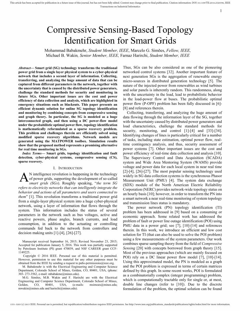
The nodal-admittance matrix of the IEEE Standard-118 Bus

is shown in Fig. 1. We see that this matrix has a sparse structure.

It has been mentioned in the literature that the PN nodal-

admittance matrix can be interpreted as a weighted version of

the Laplacian matrix of the corresponding graph 𝐺(𝑆𝑁 , 𝑆𝐸) [19]

and [17]. Moreover, since the Laplacian matrix has a direct

relationship with other important structural matrices of a graph,

the nodal-admittance matrix 𝐵 can give a full description of the

power network structure; see [19] for more information on

graphs and their corresponding matrices. As a result, our goal

is to design an appropriate and fast method to determine the

structure of the matrix 𝐵 from measurements of the PN

parameters.

C. Gaussian Distribution of Parameters

In [6]-[8] it has been thoroughly discussed that due to the

load uncertainty in large-scale transmission networks and the

increasing contribution of distributed renewable sources in

smaller scale PNs, injected active and reactive powers can be

modeled as random variables. Moreover, “the injected power

can be modeled as a Gaussian random variable since it models

the superposition of many independent factors (e.g., loads) [6]”.

The aforementioned linear relationship in (3) suggests that the

difference of phasor angles (𝜃𝑖 − 𝜃𝑗) for each sample of time

across a bus can be approximated by a Gaussian random

variable as well [7]. Moreover, allowing for the fixed phasor at

the slack bus, under steady-state conditions individual phasor

angle measurements 𝜃𝑖 can be modeled as Gaussian random

variables. Consequently, we will assume that during the

observation window of a TI problem, the measurements of the

phase angle of node 𝑖 can be well approximated by Gaussian

random variables. As we will discuss in Section III, this random

behavior has an impact on the structure of the sensing matrix in

the TI problem, and it is beneficial to the performance of sparse

recovery techniques in Section IV.

Fig.1. Corresponding normalized Laplacian matrix of the standard IEEE

118 Bus.

III. SPARSE TOPOLOGY IDENTIFICATION

We now focus on the problem of recovering the topology

matrix 𝐵 from vectors of measurements 𝑝 and 𝜃 (see (5)), or

equivalently, 𝑞 and 𝑣 (see (6)). A key assumption in our work

is that the SG can be considered as a sparse interconnected

system. This assumption is based on a survey of articles and

standard power network models found in software and

toolboxes such as MATPOWER. We observe that the regular

maximum connectivity level of a bus in a network is typically

less than 5-10%, especially in very large power transmission

systems. For example, the highest connectivity level of a bus in

IEEE 30 bus is 6 (10%), in IEEE 118 bus is 9 (7%) and in IEEE

2383 is 9 (0.3%). This means that each column in the nodal-

admittance matrix satisfies the definition of a sparse signal

(Section III-B). This sparsity helps us formulate TI as a sparse



4

recovery problem, which as supported by the theory of

Compressive Sensing, can be solved with a small set of

measurements in a fast and accurate way using SRP algorithms.

If the sparsity assumption is violated, however, the performance

of the algorithm will suffer. The formulation of TI as a SRP is

presented in Section III-A. Section III-B gives a short

background on CS. Finally, in Section III-C we introduce the

types of the SRP solvers used in this work.

A. Sparse Setup of Topology Identification Problem

Given an interconnected PN of 𝐾 buses, let the phase angle

and active power measurements of 𝑖𝑡ℎ bus be associated with

the following time series of 𝑀 sample times:

𝑝𝑖(𝑡) 𝑓𝑜𝑟 𝑡 = 1,2, . . . , 𝑀 (8)

𝜃𝑖(𝑡) 𝑓𝑜𝑟 𝑡 = 1,2, . . . , 𝑀 . (9)

As mentioned before, in the DC model, the (active or

reactive) power injected into a distinct bus 𝑖 follows the

superposition law (3) and (4). Since (4) cannot be validated

properly in some practical situations, we prefer to use (3) to

formulate the sparse TI problem. This means that, for each node

𝑖 in the network and at each sample time 𝑡, we have

𝑝𝑖(𝑡) = ∑ 𝑝𝑖𝑗𝑗 (𝑡) = ∑ 𝑏𝑖,𝑗𝑗𝜖𝛮𝑖

(𝜃𝑖(𝑡) − 𝜃𝑗(𝑡)) . (10)

As mentioned before, 𝑏𝑖,𝑗 is the susceptance along the line 𝑙𝑖,𝑗

under the DC model, and 𝛮𝑖 is the set of neighbor buses

connected directly to bus 𝑖. If we write 𝑏𝑖,𝑗 = 0 for 𝑗 ∉ 𝛮𝑖, we

can extend (10) as follows:

𝑝𝑖(𝑡) = ∑ 𝑝𝑖𝑗𝑗 (𝑡) = ∑ 𝑏𝑖,𝑗𝑗𝜖𝑆𝐾

𝑖 (𝜃𝑖(𝑡) − 𝜃𝑗(𝑡)) + 𝑢𝑖(𝑡) + 𝑒𝑖(𝑡), (11)

where 𝑆𝐾𝑖 is the set of all nodes in the network except node 𝑖 (so

the set 𝑆𝐾𝑖 contains 𝐾 − 1 nodes), 𝑢𝑖 is a possible leakage of

active power in node 𝑖 itself, and 𝑒𝑖 is the measurement noise.

Since we assume data is collected at 𝑀 sample times, we can

use matrix-vector notation to write

𝑝𝑖 = 𝐴𝑖𝑦𝑖 + 𝑢𝑖 + 𝑒𝑖, (12)

where, 𝑝𝑖 , 𝑢𝑖 , 𝑒𝑖𝜖𝑅𝑀. In equation (14) we have

𝐴𝑖 = [𝑎1,𝑖𝑇 , … , 𝑎𝑖−1,𝑖

𝑇 , 𝑎𝑖+1,𝑖𝑇 , . . . , 𝑎𝐾,𝑖

𝑇 ] 𝜖 𝑅𝑀×𝐾−1 (13)

𝑎𝑗,𝑖𝑇 = (𝜃𝑖(𝑡) − 𝜃𝑗(𝑡)) 𝜖𝑅𝑀 𝑓𝑜𝑟 𝑡 = 1,2, . . . , 𝑀 (14)

𝑦𝑖 = [𝑏𝑖,1, … , 𝑏𝑖,𝑖−1, 𝑏𝑖,𝑖+1, . . . , 𝑏𝑖,𝐾]𝑇

𝜖𝑅𝐾−1. (15)

Each column of the matrix 𝐴𝑖 represents the difference of phase

angles between node 𝑖 and one node 𝑗𝜖𝑆𝐾𝑖 in the network across

𝑀 samples of time. As discussed in Section II-C, this difference

can be modeled as a Gaussian random variable. The vector 𝑦𝑖

is a sparse vector, with all of its elements equal to zero except a

small portion, which are located in those positions

corresponding the (few) neighbors of node 𝑖. Summing over 𝑢𝑖

and 𝑒𝑖 (modeled as a vector of white Gaussian noise), we reach

the following equation for each individual bus:

𝑝𝑖 = 𝐴𝑖𝑦𝑖 + 𝜂𝑖 . (16)

1 The notation in this Section matches that in Section III-A, except for

convenience we suppose the unknown vector 𝑦 has length 𝐾 rather than 𝐾 − 1.

The TI problem can be viewed as the estimation of all vectors

{𝑦𝑖}𝑖=1𝐾 that best match the observed measurements {𝑝𝑖}𝑖=1

𝐾 . In

order to solve such a problem, we can define the following

optimization problem:

𝑚𝑖𝑛{�̂�𝑖}𝑖=1

𝐾∑ ‖𝐴𝑖�̂�𝑖 − 𝑝𝑖‖2

2𝐾𝑖=1 . (17)

Problem (17) can be solved individually for each node 𝑖. If 𝐴𝑖 is full rank, the number of measurements 𝑀 exceeds the

number of unknowns 𝐾 − 1, and the variance of the noise

vector, 𝜂𝑖, is small enough, this optimization problem can be

solved using Least Square (LS) techniques. Since the value of

𝐾 depends on the number of buses in the grid, a large number

of measurements 𝑀 will be needed to solve this problem in the

case of large power grids. In order to avoid this problem, we

suggest using sparse recovery techniques [20] to solve for the

vectors {𝑦𝑖}𝑖=1𝐾 . Since each vector 𝑦𝑖 is sparse, we can view the

goal in (16) as recovering an S-sparse vector 𝑦𝑖𝜖𝑅𝐾−1 from a

set of observations 𝑝𝑖𝜖𝑅𝑀, where 𝐴𝑖𝜖𝑅𝑀×𝐾−1 is the sensing

matrix, 𝜂𝑖𝜖𝑅𝑀 is a vector of white Gaussian noise, and 𝑆 is the

number of nodes which are directly connected to the one

individual node 𝑖 for which we are solving the problem. In

general we want 𝑀 ≪ 𝐾 so the problem can be solved using a

reasonable set of observations in huge power grids. After

solving this problem for each sparse vector 𝑦𝑖 corresponding to

each node 𝑖, we can concatenate all of the sparse vectors

together, form the weighted Laplacian matrix 𝐵, and the process

is completed. Because 𝜃𝑖(𝑡) − 𝜃𝑗(𝑡) = 0 for 𝑖 = 𝑗, 𝑆𝐾𝑖 should

include 𝐾 − 1 nodes; in other words, we should keep the node

𝑖 out of 𝑆𝐾𝑖 since it produces a vector of zeros in the

corresponding column of the matrix 𝐴𝑖. Thus, we cannot

directly calculate the value of the parameter 𝐵𝑖𝑖 from the

recovered vector 𝑦𝑖; however, regarding the aforementioned

definition of the matrix 𝐵,

𝐵𝑖𝑖 = ∑ 𝑏𝑖,𝑗𝑗𝜖𝛮𝑖 . (18)

Thus, after recovering the vector 𝑦𝑖 , 𝐵𝑖𝑖 can be easily calculated.

In the next section, we briefly give a summary of the required

CS and SRP background and concepts used in interpreting and

solving (16) as an SRP.

B. CS Background and Related Concepts

Definition 1 (Sparse Signal): An S-sparse signal 𝑦𝜖𝑅𝐾 is a

signal of length 𝐾 with 𝑆 non-zero entries where 𝑆 < 𝐾 (in

many cases (𝑆 ≪ 𝐾).1

Intuitively, the SRP is an optimization problem in which the

goal is to recover an S-sparse signal 𝑦𝜖𝑅𝐾 from a set of linear

observations (measurements) 𝑝 = 𝐴𝑦 𝜖𝑅𝑀 where 𝐴𝜖𝑅𝑀×𝐾 is

the sensing matrix with 𝑀 < 𝐾 (in many cases 𝑀 << 𝐾).

Typically in CS, the number of measurements 𝑀 will be

proportional to the sparsity level 𝑆 of the signal 𝑦 to be

recovered. For example, it is known that when the sensing

matrix 𝐴 is drawn randomly from a suitable distribution (i.e.,

the measurement protocol is random), with high probability any

𝑆-sparse signal 𝑦 can be recovered from the measurements 𝑝 =𝐴𝑦 if the number of measurements 𝑀 is merely proportional



5

𝑆 𝑙𝑜𝑔 (𝐾

𝑆). This number of measurements can be significantly

smaller than the overall signal length 𝐾, and is only greater than

the fundamental limit 𝑆 by a logarithmic factor; one can

interpret this logarithmic factor as the price that should be paid

for not knowing the locations of the sparse coefficients in

advance. Remarkably, assuming the signal 𝑦 to be exactly

sparse and the measurements 𝑝 = 𝐴𝑦 to be noise-free, this

recovery is exact. If the signal to be recovered is nearly sparse

(compressible2) or if the measurements are noisy, this recovery

is provably robust. Compressible signals appear in variety of

applications such as when CS-based techniques are used for

MRI; in many such applications, approximate signal recovery

is sufficient. However, in our work each column of the matrix

𝐵 is exactly sparse. Due to the underdetermined nature of this

recovery problem (i.e., since 𝑀 < 𝐾), the null space of the

sensing matrix 𝐴 is non-trivial; therefore, we have infinitely

many candidate solutions to the system of equations 𝑝 = 𝐴𝑦.

However, under certain conditions on the sensing matrix 𝐴, CS-

based recovery methods can be guaranteed to efficiently find

the candidate solution that is sparse enough. The following

definitions and theorems provide examples of such conditions;

for more discussion and technical proofs and details please refer

to [20]-[22] and references therein.

Definition 2 (Coherence): The coherence of an 𝑀 × 𝐾 matrix

𝐴 with normalized columns 𝑎1, 𝑎2, … , 𝑎𝐾 is defined as follows:

𝜇𝐴 = 𝑚𝑎𝑥1≤𝑚,𝑛≤𝐾,𝑚≠𝑛

|⟨𝑎𝑚, 𝑎𝑛⟩| . (19)

The coherence of an 𝑀 by 𝐾 matrix 𝐴 is a value in the interval

[1

√𝐾, 1].

Definition 3 (Restricted Isometry Property): An 𝑀 by 𝐾

sensing matrix 𝐴 satisfies the Restricted Isometry Property

(RIP) of order 𝑆 if

(1 − 𝛿𝑆)‖𝑦‖22 ≤ ‖𝐴𝑦‖2

2 ≤ (1 + 𝛿𝑆)‖𝑦‖22 (20)

holds for all coefficient vectors 𝑦 with ‖𝑦‖0 ≤ 𝑆 where

𝛿𝑆𝜖(0,1) is known as the isometry constant of order 𝑆.

Theorem 1 (Coherence-based recovery guarantee): Suppose

𝑦 is S-sparse and let 𝑝 = 𝐴𝑦. If

𝜇𝐴 <1

2𝑆−1 , (21)

then �̂� = 𝑦 is the unique solution to 𝑝 = 𝐴�̂� having sparsity 𝑆

or less. The smaller the coherence of 𝐴, the larger the permitted

value of 𝑆, and the broader the class of signals that can be

recovered. Roughly, what these conditions require is that any

two subsets of columns of the sensing matrix 𝐴 must be almost

orthogonal to each other.

Theorem 2 (RIP-based recovery guarantees): Suppose 𝐴

satisfies the RIP of order 2𝑆 with 𝛿2𝑠 < 0.4651. Let 𝑝 = 𝐴𝑦 +𝜂 be noisy measurements of a vector 𝑦. Then for any S-sparse

vector 𝑦, (22) correctly returns �̂� = 𝑦 given 𝑝:

�̂� = 𝑎𝑟𝑔𝑚𝑖𝑛�́�

‖�́�‖1 𝑠𝑢𝑏𝑗𝑒𝑐𝑡 𝑡𝑜 ‖𝑝 − 𝐴�́�‖2 < 휀. (22)

Moreover, for any vector 𝑦, if 휀 ≥ ‖𝜂‖2, then the solution �̂� to

(22) obeys:

2 The nearest 𝑆-sparse signal to 𝑥, 𝑥𝑠, can be obtained simply by keeping the

𝑆 largest entries of 𝑥 and setting all remaining entries to 0. If 𝑥 is exactly 𝑆-

‖𝑦 − �̂�‖2 ≤ 𝐶1‖𝑦−𝑦𝑆‖1

√𝑆+ 𝐶2휀 , (23)

where 𝐶1 and 𝐶2 depend only on the matrix isometry constant.

The vector 𝑦𝑆 is the closest 𝑆-sparse approximation to 𝑦. The

optimization (22) is widely known as Basic Pursuit Denoising

(BPDN) and is an SRP. In the next section, we briefly introduce

several SRP solvers which are used in this work. By

generalizing these methods, we will introduce new adaptable

strategies in order to address the practical challenges involved

in solving the sparse TI problem.

C. Sparse TI Structure and Data Correlation Issues

In general, the standard techniques for solving SRPs can be

categorized into two major groups: greedy algorithms and

algorithms based on convex optimization. In this work we will

use the popular greedy Orthogonal Matching Pursuit (OMP)

algorithm (see Algorithm 1) and the convex optimization

algorithm known as LASSO. The LASSO estimator is defined

as follows:

�̂� = 𝑎𝑟𝑔𝑚𝑖𝑛�́�‖𝑝 − 𝐴�́�‖22 + 𝜆‖�́�‖1 . (24)

This can be viewed as the Lagrangian form of the BPDN

problem (24).

Algorithm 1 Orthogonal Matching Pursuit - OMP require: matrix 𝑨, measurements 𝒑 , stopping criterion

initialize: 𝒓𝟎 = 𝒑, 𝒚𝟎 = 𝟎, 𝒍 = 𝟎, 𝑺𝑼𝑷𝟎 = ∅ repeat

1.match: 𝒉𝒍 = 𝑨𝑻𝒓𝒍 2.identify support indicator:

𝒔𝒖𝒑𝒍 = {𝒂𝒓𝒈𝒎𝒂𝒙𝒋|𝒉𝒍(𝒋)|}

3.update the support:

𝑺𝑼𝑷𝒍+𝟏 = 𝑺𝑼𝑷𝒍 ∪ 𝒔𝒖𝒑𝒍 4.update signal estimate:

𝒚𝒍+𝟏 = 𝒂𝒓𝒈𝒎𝒊𝒏𝒛: 𝒔𝒖𝒑𝒑(𝒛)⊆𝑺𝑼𝑷𝒍+𝟏‖𝒑 − 𝑨𝒛‖𝟐

𝒓𝒍+𝟏 = 𝒑 − 𝑨𝒚𝒍+𝟏

𝒍 = 𝒍 + 𝟏 Until stopping criterion met

output: �̂� = 𝒚𝒍

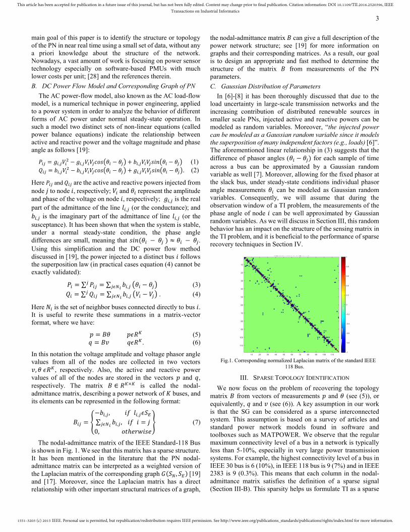
a. Structured Sparsity

By inspection of the columns of the Laplacian matrices of

standard IEEE test-beds (Fig.1 and Fig.2) we see that the

columns tend to exhibit a clustered sparse structure: the column

vectors not only contain few nonzero elements (i.e., they are

sparse), but the nonzero elements tend to occur in nearly

adjacent positions. In the case of the IEEE Standard-14 Bus or

IEEE Standard-30 Bus, columns 2, 5 and 6 or columns 6 and 10

can be taken as clear examples, respectively. Since in a real PN,

nodes and lines are ordered based on their position in the

network, and commonly the neighbor nodes are connected

through neighbor lines (except in special cases), it is realistic in

practice to assume that nodes have an ordering that lends itself

to clustered sparsity. In one of our recent works [21], we have

used this (17) formulation in addition to reweighted 𝑙1

algorithm to exploit the concentration of the nonzero elements

to the main diagonal besides the clustered structure in the

signal.

sparse, then 𝑥 = 𝑥𝑠. If the distance from 𝑥 to 𝑥𝑠 is small (but not necessarily

zero), 𝑥 is said to be compressible.



6

Fig.2. Corresponding Laplacian matrices of the standard IEEE test-beds;

a) IEEE 14 Bus and b) IEEE 30 Bus (Scaled between [-1, 1]).

Definition 4 (Clustered sparsity): We refer to a signal 𝑦 ∈ 𝑅𝐾

as (S;C)-clustered sparse if the total number of nonzero

coefficients is 𝑆 and all nonzero coefficients are distributed

within 𝐶 disjoint clusters (the locations and sizes of the clusters

are arbitrary).

Figure 3 shows the difference between the general structure

of an 𝑆-sparse signal (Fig. 3a) and a clustered-sparse signal

(Fig. 3b).

Modified Clustered OMP

Clustered OMP is a generalized version of the traditional

greedy method OMP. COMP modifies the support

identification step of OMP in order to improve the SRP results

whenever we expect clustered sparsity in the signal to be

recovered [23]. In Section IV, we show how COMP offers

improved recovery of clustered sparse signals. The step-wise

description of COMP (from [23]) is given in Algorithm 2.

Algorithm 2 Clustered Orthogonal Matching Pursuit- COMP require: matrix A, measurements 𝒑 , maximum cluster size m, stopping criterion

initialize: 𝒓𝟎 = 𝒑, 𝒚𝟎 = 𝟎, 𝒍 = 𝟎, 𝑺𝑼𝑷𝟎 = ∅

repeat


𝒔𝒖𝒑𝒍 = {𝒂𝒓𝒈𝒎𝒂𝒙𝒋|𝒉𝒍(𝒋)|}

3.extend support

𝒔𝒖𝒑 ̂ 𝒍 = {𝒔𝒖𝒑𝒍 − 𝒎 + 𝟏, … , 𝒔𝒖𝒑𝒍, … , 𝒔𝒖𝒑𝒍 + 𝒎 − 𝟏} 4.update the support:

𝑺𝑼𝑷𝒍+𝟏 = 𝑺𝑼𝑷𝒍 ∪ 𝐬𝐮𝐩 ̂ 𝒍 5.update signal estimate:


𝒓𝒍+𝟏 = 𝒑 − 𝑨𝒚𝒍+𝟏



In order to improve the handling of border effects, we make a

slight modification to Step 3 of COMP as follows:

3.1. finding the boundaries of the support

Upper Bound = 𝒎𝒊𝒏((𝒔𝒖𝒑𝒍 + 𝒎 − 𝟏), 𝟏))

Lower bound = 𝒎𝒂𝒙(𝒔𝒖𝒑𝒍 − 𝒎 + 𝟏), 𝑵)

3.2. modified extend support:

𝒔𝒖𝒑𝒍 = {𝑳𝒐𝒘𝒆𝒓 𝒃𝒐𝒖𝒏𝒅 , … , 𝒔𝒖𝒑𝒍, … , 𝑼𝒑𝒑𝒆𝒓 𝑩𝒐𝒖𝒏𝒅 }

We call the resulting algorithm Modified COMP (MCOMP).

b. Data Correlation Issue

Even though graph data analytics are essential for gaining

insight into big networks, large-scale interconnected network

processing is complex because of its graph-specific challenges,

including complicated correlations among data entities, highly

skewed distributions, and so on. Considering large-scale

interconnected power networks, the possible correlation among

the recorded data from the nodes (especially from neighboring

nodes) is an issue in sparse TI since it may result in highly

coherent sensing matrices 𝐴. As noted in Theorem 1, high

coherence can have an undesirable effect on the performance of

SRP solvers. Recently, two new techniques named Band–

exclusion (B) and Local Optimization (LO) have been

developed in [25] in order to help address the high coherence

issue in sparse signal recovery. The BLO technique known as

BLOOMP can be interpreted as adding an additional constraint

on the support selection step in OMP to prevent the algorithm

from picking highly correlated indexes in the estimated support

of the sparse signal [25]. Within this algorithm a new concept

termed the coherence band is defined. The coherence band (𝑐𝑏)

and related concepts are defined as follows: for some tolerance

𝛼 ≥ 0,

𝐵𝛼(𝜆) = {𝑖| |⟨𝑎𝑖, 𝑎𝜆⟩| > 𝛼} (25)

𝐵𝛼(𝛬) =∪𝜆𝜖𝛬 𝐵𝛼(𝜆) (26)

𝐵𝛼(2)(𝜆) = 𝐵𝛼(𝐵𝛼(𝜆)) =∪𝑗𝜖𝐵𝛼(𝜆) 𝐵𝛼(𝑗) (27)

𝐵𝛼(2)(𝛬) = 𝐵𝛼(𝐵𝛼(𝛬)) =∪𝜆𝜖𝛬 𝐵𝛼

(2)(𝜆). (28)

However, there is an issue with applying such a method in the

sparse TI problem. Due to nature of this method, whenever the

correlation between two columns of the sensing matrix is high

one of the corresponding positions will not be selected within

the true support. On the other side, as it has been mentioned

before, in TI the positions of the nonzero elements of a signal

vector are typically clustered. Since correlation in a sensing

matrix tends to be highest for columns corresponding to

neighboring nodes, this means that applying the BLOOMP

method may cause us to miss some nonzero elements of the

signal vector. In order to deal with this problem, we suggest an

algorithm composed of BLOOMP and MCOMP that we refer

to as BLOMCOMP (Algorithm 3); this algorithm adds the pre-

knowledge of clustered sparsity to BLOOMP. This

modification prevents us from losing nonzero neighbor

elements within a cluster. In addition to band-exclusion, LO is

used in BLOMCOMP as a residual-reduction technique (for

more information please refer to [25]).

Algorithm 3 Band-excluded Locally Optimized MCOMP

(BLOMCOMP) require: matrix 𝑨 , measurements 𝒑 , Coherence band 𝜶 > 𝟎 , maximum

cluster size 𝒎, stopping criterion

initialize: 𝒓𝟎 = 𝒑, 𝒚𝟎 = 𝟎, 𝒍 = 𝟎, 𝑺𝑼𝑷𝟎 = ∅

repeat


𝒔𝒖𝒑𝒍 = {𝒂𝒓𝒈𝒎𝒂𝒙𝒋|𝒉𝒍(𝒋)|} , 𝒋 ∉ 𝑩𝜶

(𝟐)(𝑺𝑼𝑷𝒍−𝟏)

3.update the support:

Upper Bound = 𝒎𝒊𝒏((𝒔𝒖𝒑𝒍 + 𝒎 − 𝟏), 𝟏))

Lower bound = 𝒎𝒂𝒙(𝒔𝒖𝒑𝒍 − 𝒎 + 𝟏), 𝑲)

𝒔𝒖𝒑 ̂ 𝒍 = {𝑳𝒐𝒘𝒆𝒓 𝒃𝒐𝒖𝒏𝒅 , … , 𝒔𝒖𝒑𝒍, … , 𝑼𝒑𝒑𝒆𝒓 𝑩𝒐𝒖𝒏𝒅 } 𝑺𝑼𝑷𝒍+𝟏 = 𝑳𝑶(𝑺𝑼𝑷𝒍 ∪ {𝒔𝒖𝒑 ̂ 𝒍}) 4.update signal estimate:


𝒓𝒍+𝟏 = 𝒑 − 𝑨𝒚𝒍+𝟏



(b) (a)



7

Local Optimization Procedure require: 𝑨, 𝒚 , Coherence band 𝜶 > 𝟎, 𝑺𝑼𝑷𝟎 = ∪ {𝒔𝒖𝒑 ̂ 𝒊} 𝒇𝒐𝒓 𝒊 = 𝟏: 𝒌+1

repeat: for 𝒊 = 𝟏: 𝒌+1

1. 𝒚𝒊 = 𝒂𝒓𝒈𝒎𝒊𝒏𝒛:𝒔𝒖𝒑𝒑(𝒛)=(𝑺𝑼𝑷𝒊−𝟏 \{𝒔𝒖𝒑 ̂ 𝒊}) ∪ {𝝀𝒊},𝝀𝒊𝝐𝑩𝜶({𝒔𝒖𝒑 ̂ 𝒊})‖𝒑 − 𝑨𝒛‖𝟐

2. 𝑺𝑼𝑷𝒊 = 𝒔𝒖𝒑𝒑(𝒚𝒊)

output: 𝑺𝑼𝑷𝒌+𝟏

Fig.3 (a) Structure of a 6-sparse signal. (b) A (25;5)-clustered-sparse signal.

(c) The average value of Coherence 𝜇𝐴 vs # of measurements 𝑀 over all 118

corresponding sensing matrices '𝐴' for all of the nodes in the IEEE 118-Bus.

IV. SIMULATION RESULTS AND DISCUSSION

A. Setup

In this section, we test the proposed method for recovering

the topology of an SG using compressive observations (𝑀 < 𝐾)

collected from the system parameters. We see that the

probability of successful recovery varies for different nodes in

the network based on the local pattern of sparsity. In these

simulations, we use the IEEE Standard-30 Bus, 118 Bus and,

2383 as case studies. These three PNs include 30 Buses and 47

power transmission lines, 118 Buses and 186 lines, and 2383

Buses and 2896 lines, respectively, and their detailed

specifications have been fully described in the MATPOWER

toolbox [18]. To generate the data, we first feed the system with

Gaussian demand and simulate the PN. The MATPOWER [18]

toolbox is used for solving the power flow equations in various

demands and the resulting phase angle and active power

measurements are applied as the input to the SRP. Finally, 1-

2% white noise has been added to measurement vectors

randomly.

Each column of the matrix 𝐵 represents one of the sparse

vectors 𝑦𝑖 which we attempt to recover by solving an SRP. For

the IEEE Standard-118 Bus, Fig. 3c shows how the coherence

(19) of the corresponding sensing matrix 𝐴 changes as the

number of measurements 𝑀 increases; curves are averaged over

1000 realizations of the network and over all 118 nodes. This

coherence measure appears to approach a non-zero asymptote

as the number of measurements increases. As has been

mentioned before, the smaller the coherence metric, the larger

the sparsity 𝑆 of signals that can be recovered. One class of

matrices well known to have low coherence are random

Gaussian matrices. As mentioned in Section II-C and in the

literature such as [6]-[8], due to the load uncertainty and the

aggregation of the renewables in SGs, the difference of the

phase angles across a bus can be approximated by a Gaussian

random variable. Moreover, in the SRP formulation in Section

III-A, the sensing matrix is formed by the variation in bus phase

angles. Thus, the closer the behavior of the phase angles is to

being Gaussian, the better one might expect the sparse recovery

algorithms to perform.

B. Results

Within the network graph, SRP solvers exhibit different

recovery performance on different nodes for a given number of

measurements, mainly because of the following two factors.

The first factor is the sparsity level of the signal 𝑦𝑖 (or in our

PN, the in-degree, or the number of connected links to a bus),

and the second factor is the presence of a possible structure in

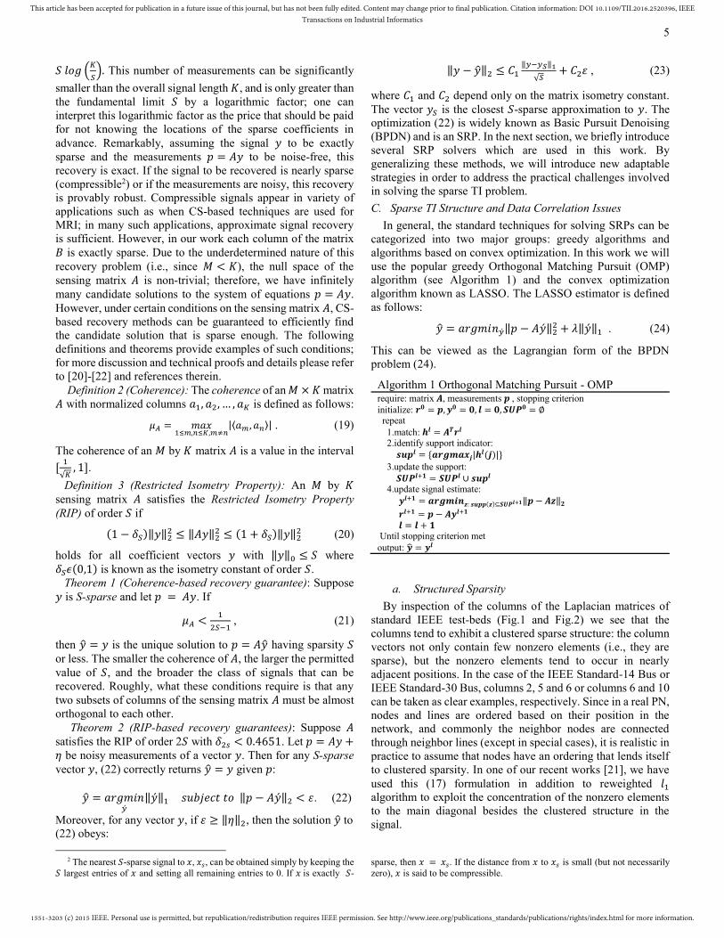
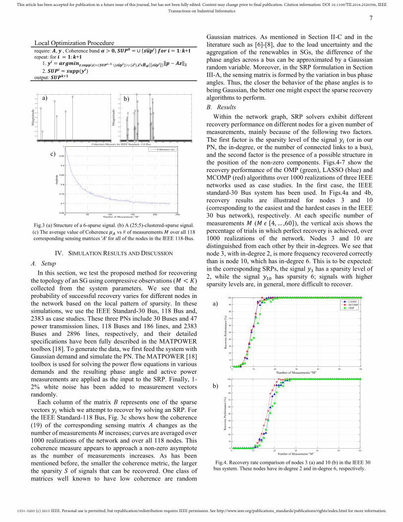
the position of the non-zero components. Figs.4-7 show the

recovery performance of the OMP (green), LASSO (blue) and

MCOMP (red) algorithms over 1000 realizations of three IEEE

networks used as case studies. In the first case, the IEEE

standard-30 Bus system has been used. In Figs.4a and 4b,

recovery results are illustrated for nodes 3 and 10

(corresponding to the easiest and the hardest cases in the IEEE

30 bus network), respectively. At each specific number of

measurements 𝑀 (𝑀 𝜖 {4, … ,60}), the vertical axis shows the

percentage of trials in which perfect recovery is achieved, over

1000 realizations of the network. Nodes 3 and 10 are

distinguished from each other by their in-degrees. We see that

node 3, with in-degree 2, is more frequency recovered correctly

than is node 10, which has in-degree 6. This is to be expected:

in the corresponding SRPs, the signal 𝑦3 has a sparsity level of

2, while the signal 𝑦10 has sparsity 6; signals with higher

sparsity levels are, in general, more difficult to recover.

Fig.4. Recovery rate comparison of nodes 3 (a) and 10 (b) in the IEEE 30 bus system. These nodes have in-degree 2 and in-degree 6, respectively.

a)

c)

b)

a) b)



8

Another important factor, which affects the SRP solver’s

performance, is the existence of a possible clustered structure

in the sparse signals to be recovered. As we have mentioned,

MCOMP is an extended version of OMP, which has been

adapted to exploit the knowledge that the non-zero entries of

the signal appear in clusters. The structured sparsity in the

columns of the matrix 𝐵 can be used to improve the recovery

performance. Figs.4a and 4b show how the presence of

clustered sparsity helps the MCOMP algorithm to outperform

the LASSO and OMP, especially in the case of node 10, where

𝑦10 is a (6, 4)-clustered sparse signal and the in-degree of the

node (or the number of nonzero elements of the signal to be

recovered) is larger.

Fig.5. Recovery rate comparison of nodes 74, 59, and 49 in the IEEE 118-Bus,

with in-degree 2, 5, and 9 respectively.

In order to compare the performance over more complicated

cases, the IEEE Standard-118 Bus and 2383 Bus systems have

also been used for modeling the PN. In the IEEE 118 bus, we

focus on recovering the connections to nodes 74 (which has in-

degree 2), 49 (in-degree 9), and 59 (in-degree 6). In the IEEE

2383 bus, we focus on nodes 3 (in-degree 3) and 1920 (in-

degree 9). From the sparsity level viewpoint, 𝑦49 and 𝑦1920

correspond to the most complicated signals 𝑦𝑖 to be recovered

in the two networks, respectively. Recovery results are again

shown over 1000 realizations of the corresponding network.

Figs.5a-c show the recovery results for the IEEE 118 Bus

network. As might be expected, we see that node 74 (with in-

degree 2) is more likely to be recovered from a given number

of measurements than is node 59 (in-degree 6). Node 49 (with

in-degree 9) is the most difficult to recover. These plots also

show how MCOMP outperforms LASSO and OMP in the case

of node 49, where 𝑦49 is a (9, 5)-clustered sparse signal and the

in-degree of the node (or the number of nonzero elements of the

signal to be recovered) is larger. On node 59 (where the

corresponding signal 𝑦59 is a (6, 3)-clustered sparse signal)

MCOMP again outperforms OMP and LASSO. On node 74

(where 𝑦74 has no clustered sparsity), LASSO is the best

performing algorithm.

Moreover, Fig.6.a and b are representing the recovery

performance of each of 3 SRP solvers for 3-sparse node 3 and

9-sparse node 1920 in IEEE 2383 Bus network. Due to the

larger scale of this network, we generally need more

measurements to achieve the perfect recovery for any

individual node compared to smaller networks like the IEEE

118 Bus. As it has been mentioned before, the number of

measurements needed for full recovery depends on both the

sparsity level and the original dimension of the signal 𝑦 (here,

the dimension 𝐾 equals the number of buses in our sparse TI

problem); specifically, 𝑀 must be at least proportional to

𝑆 𝑙𝑜𝑔(𝐾/𝑆). As a rough rule of thumb, in many applications,

when the sensing matrix has low coherence, one observes

perfect recovery when 𝑀 ≈ 4𝑆. However, as the dimension 𝐾

grows, it becomes necessary to take more measurements. For

example, in the case of the IEEE 118 Bus, node 49 has in-degree

9, and perfect recovery is possible when 𝑀 ≈ 50. In the case of

the IEEE 2383 network, node 1920 again has in-degree 9, but

perfect recovery is not possible until 𝑀 ≈ 80.

Fig.6. Recovery rate comparison of nodes 3 and 1920 in the IEEE standard 2383 network. Nodes 3 and 1920 have in-degree 3 and 9, respectively.

b)

a)

OMP

a)

b)

c)



9

Comparing the results from different size networks it is clear

that number of measurements required for perfect recovery is

affected less by the network size than by the sparsity level of

the corresponding signal 𝑦𝑖 to be recovered. Taking fewer

measurements reduces the recovery performance of any SRP

solver; however, the LASSO and MCOMP generally show

better recovery performance than OMP. Moreover, we cannot

recover the nodes with higher in-degrees (such as node 49,

where 𝑦49 is a (9, 5)-clustered sparse signal) until 𝑀 is large

enough that the PN coherence metric reaches a suitably small

level, and if such a level were never to be reached, we might be

limited in the degree of nodes that we could recover with these

techniques.

Finally, in order to highlight the effect of the data correlation

issue in addition to the impact of clustered sparsity, we have

examined the recovery results for two other clustered sparse

signals in the IEEE 118 bus: signal 𝑦37 which is a (6, 2)-

clustered sparse signal, and signal 𝑦80 which is an (8, 4)-

clustered sparse signal. In general, as one should expect 𝑦37 to

be easier to recover compared to 𝑦80. In order to evaluate the

results we define the interconnection order (𝐼𝑂) for node 𝑖 as

follows:

𝐼𝑂(𝑖) = ∑ 𝑖𝑛 − 𝑑𝑒𝑔𝑟𝑒𝑒(𝑗)𝑗𝜖𝛮𝑖 (29)

Node 37 has 6 direct neighbors and 𝐼𝑂(37) = 17; node 80

has 8 direct neighbors and 𝐼𝑂(80) = 22. The interconnection

order can be interpreted as a factor that can reflect the level of

data correlation within a specific bus versus the rest of the

network; however, it will not be the only factor. Fig.7 illustrates

how BLOMCOMP outperforms MCOMP, OMP and LASSO

in the case of node 80, where we face a more complicated and

interconnected local topology and a higher coherence in the

corresponding sensing matrix.

Fig.7. Recovery rate comparison of nodes 37 and 80 in the IEEE 118-Bus.

An initial value of m = 4 is chosen in MCOMP and BLOMCOMP.

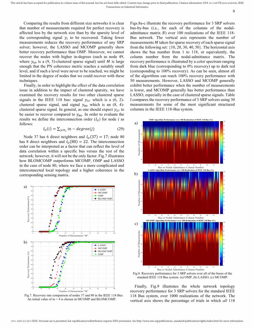
Figs.8a-c illustrate the recovery performance for 3 SRP solvers

bus-by-bus (i.e., for each of the columns of the nodal-

admittance matrix 𝐵) over 100 realizations of the IEEE 118-

Bus network. The vertical axis represents the number of

measurements 𝑀 taken for sparse recovery of each sparse signal

from the following set: {10, 20, 30, 40, 50}. The horizontal axis

shows the bus number from 1 to 118, or equivalently, the

column number from the nodal-admittance matrix. The

recovery performance is illustrated by a color spectrum ranging

from dark blue (corresponding to 0% recovery) up to dark red

(corresponding to 100% recovery). As can be seen, almost all

of the algorithms can reach 100% recovery performance with

50 measurements. However, LASSO and MCOMP generally

exhibit better performance when the number of measurements

is lower, and MCOMP generally has better performance than

LASSO, especially in the case of clustered sparse signals. Table

I compares the recovery performance of 3 SRP solvers using 30

measurements for some of the most significant structured

columns in the IEEE 118-Bus system.

Fig.8. Recovery performance for 3 SRP solvers over all of the buses of the

standard IEEE 118 Bus system: (a) OMP, (b) LASSO, (c) MCOMP.

Finally, Fig.9 illustrates the whole network topology

recovery performance for 3 SRP solvers for the standard IEEE

118 Bus system, over 1000 realizations of the network. The

vertical axis shows the percentage of trials in which all 118

b)

c)

a)

a)

b)



10

columns of the nodal-admittance matrix 𝐵 (and, as a result, the

whole network topology) are perfectly recovered. This figure

also shows that the whole network topology can typically be

recovered from 50 or fewer measurements per bus.

Table. I. Recovery performance of 3 SRP solvers using 30 measurements for

the most significant clustered sparse buses in the IEEE 118-Bus system.

Bus (Column) # OMP (%) LASSO (%) MCOMP (%)

5 90 91 100

11 92 100 98

12 52 54 51

15 85 93 100

17 74 71 88

56 89 92 100

62 92 99 99

85 74 92 99

100 31 32 78

105 90 90 100

Fig.9. Whole network topology recovery performance for 3 SRP solvers

for the standard IEEE 118 Bus system over 1000 realizations of the network.

V. CONCLUSIONS

In this study, we explore the topology identification problem

for smart grids. The DC power flow model, graph theory, and

sparse recovery techniques from compressive sensing are

composed in order to address the following challenges in

topology identification and line outage localization of

transmission lines: 1) the computational complexity of data

collection and analysis procedures in large scale SGs; 2) the

effect of distributed generation systems such as wind turbines

or PV cells; and 3) the uncertainty of system states and

parameters caused by the nonlinear and stochastic behavior of

loads. The proposed method models the SG as an

interconnected graph. Next, using an approximated version of

the AC power-flow model (a DC model) under the probabilistic

power flow regime, the TI problem is mathematically

formulated as an optimization problem.

Finally, due to the sparse nature of this optimization problem

the TI can be interpreted as an SRP, which can efficiently be

solved using SRP solvers such as greedy (OMP, MCOMP) or

optimization based (LASSO) algorithms. We have discussed

important concepts from CS such as coherence and its behavior

in a sparse representation of the TI problem for IEEE standard

networks. Network models have been generated using the

MATPOWER toolbox and standard IEEE test-beds. The main

advantage of the presented method is that this sparse

reformulation of the TI problem relies only on the

measurements from the system parameters and does not need

any a priori information about the topology of the network. In

fact, in our technique, the output of the SRP solver methods is

the structure or topology matrix of the network itself. Case

studies using standard IEEE standard test-beds have shown that

the proposed method represents a promising new strategy for

topology identification, fault detection, and monitoring using

only a small set of observations from some of the bus

parameters. This paper shows that the recovery performance of

the SRP solvers is mainly dependent on the in-degree (number

of lines connected) of each bus in the network. Moreover, the

sparse signals to be recovered often exhibit a clustered-sparse

structure, so it is possible to improve the recovery results using

SRP solvers that encourage structured sparsity. We have also

addressed the problem of correlation in the sensing matrix

among columns that are likely to belong to the signal support.

REFERENCES

[1] X.Y.Yu, C. Cecati, T. Dillon, and M. G. Simões, “The new frontier of

smart grids,” IEEE Ind. Electron. Mag., vol. 5, no. 3, pp. 49–63, Sep.

2011.

[2] V. Gungor, D. Sahin, T. Kocak, S. Ergut, C. Buccella, C. Cecati, and G.

Hancke, Smart Grid Technologies Communications Technologies and Standards” IEEE Transactions on Industrial Informatics, vol.7, no. 4, pp.

529-539, Sept. 2011.

[3] Weilin Li, Mohsen Ferdowsi, Marija Stevic, Antonello Monti, and Ferdinanda Ponci, “Cosimulation for Smart Grid Communications”,

IEEE Transactions on Industrial Informatics, vol. 10, no. 4, Nov 2014. [4] X. Fang, S. Misra, G. Xue, and D. Yang, “Smart grid-The new and

improved power grid: A survey,” IEEE Commun. Surveys Tutorials, vol.

14, no. 4, pp. 944–980, Fourth Quarter 2012. [5] Harirchi, Farnaz; Simoes, M.Godoy, Al Durra, Ahmed and Muyeen, S.M.

"Short transient recovery of low voltage-grid-tied DC distributed

generation". ECCE, 2015 IEEE, pp 1149-1155, Montreal, QC, Canada, Sept. 2015.

[6] H. Sedghi, E Jonckheere. Information and Control in Networks. In

Giacomo Como, Bo Bernhardsson, Anders Rantzer, editors, Lecture Notes in Control and Information Sciences, vol. 450, 2014, Springer

Cham Heidelberg New York Dordrecht London, Ch. 9, pp 277-297.

[7] M. He and J. Zhang. “A dependency graph approach for fault detection and localization towards secure smart grid”. IEEE Transactions on Smart

Grid, no. 2, pp. 342–351, June 2011.

[8] A. Schellenberg, W. Rosehart, and J. Aguado, “Cumulant-based probabilistic optimal power flow (P-OPF) with Gaussian and Gamma

distributions,”IEEE Trans. on Power Systems, vol. 20, pp. 773–781, May

2005. [9] V. Kekatos, G. B. Giannakis, and R. Baldick, “Grid topology

identification using electricity prices,” in Proc. IEEE Power & Energy

Society General Meeting, National Harbor, MD, Jul. 2014. [10] H. Zhu and G. B. Giannakis, “Sparse Overcomplete Representations for

Efficient Identification of Power Line Outages” IEEE Trans. on Power

Systems, vol. 23, pp. 1644-1652, Oct. 2012. [11] J.C. Chen, W.T Li, C.K. Wen, J.H. Teng, P. Ting. “Efficient identification

method for power line outages in the smart power grid”. IEEE Trans.

Power Systems, vol. 29, pp. 1788–1800, 2014. [12] Zhao and W.-Z. Song, “Distributed power-line outage detection based on

wide area measurement system,” Sensors, vol. 14, no. 7, pp. 13 114–13

133, Jan. 2014. [13] J. Wu, J. Xiong, and Y. Shi, “Efficient location identification of multiple

line outages with limited PMUs in smart grids,” IEEE Trans. Power Syst.,

vol. 30, no. 4, pp. 1659-1668, Jul 2015. [14] Wen-Tai Li, Chao-Kai Wen, Jung-Chieh Chen, Kai-Kit Wong, Jen-Hao

Teng, and Chau Yuen. “Location Identification of Power Line Outages

Using PMU Measurements with Bad Data”. arXiv:1502.05789v1 [cs.SY] 20 Feb 2015.

[15] M. Majidi, A. Arabali, and M. Etezadi-Amoli, “Fault location in

distribution networks by compressive sensing,” IEEE Trans. on Power Delivery. vol.30, no,4,pp 1761-1769, Aug 2015.

[16] Guangyu Feng, and Ali Abur. “Fault Location Using Wide-Area

Measurements and Sparse Estimation”. IEEE Trans. on Power Systems Accepted and to be published, 2016.

[17] D. B. West, Introduction to Graph Theory, 2nd ed., Prentice Hall, 2001.



11

[18] R. D. Zimmerman, C. E. Murillo-Sanchez, and R. J. Thomas, “Steady-

state operations, planning and analysis tools for power systems research and education,” IEEE Trans. on Power Systems, vol. 26, no. 1, pp. 12–19,

Feb. 2011.

[19] A. J. Wood and B. F. Wollenberg, Power Generation, Operation, and Control, 2nd ed. New York: Wiley, 1996.

[20] E.J. Candes and M.B. Wakin, “An introduction to compressive sam-

`pling”, IEEE Signal Processing Magazine, vol. 24, pp. 21–30, Mar 2008. [21] M Babakmehr, MG Simoes, MB Wakin, A Durra, F Harirchi. "Smart grid

topology identification using sparse recovery". Presented in Industry

Applications Society Annual Meeting, Oct 2015, to be reviewed in IEEE Trans of Industrial Applications.

[22] M. B. Wakin. Compressive Sensing Fundamentals. In M. Amin, editor,

Compressive Sensing for Urban Radar, pp. 1-47. CRC Press, Boca Raton, Florida, 2014.

[23] B.M. Sanandaji, T.L. Vincent, and M.B. Wakin. “Compressive Topology

Identification of Interconnected Dynamic Systems via Clustered Orthogonal Matching Pursuit”, in Proceedings of the 50th IEEE CDC-

ECC 2011, Orlando, Florida, USA, Dec. 2011, pp. 174–180.

[24] M. Babakmehr, M.G. Simões, A. Al Durra, F. Harirchi and Qi. Han. “Application of Compressive Sensing for Distributed and Structured

Power Line Outage Detection in Smart Grids”, IEEE, ACC 2015, pp

3682-3689, Chicago, Illinois, USA, July 2015. [25] A. Fannjiang, W. Liao. "Coherence Pattern–Guided Compressive Sensing

with Unresolved Grids". SIAM J. IMAGING SCIENCES, vol. 5, no. 1, pp.

179–202, 2012. [26] Debomita Ghosh, T. Ghose, and D. K. Mohanta. “Communication

Feasibility Analysis for Smart Grid with Phasor Measurement Units”. IEEE Transactions on Industrial Informatics, vol. 9, no. 3, pp 1486-1496,

Aug 2013.

[27] Ayman I. Sabbah, Student Member, IEEE, Amr El-Mougy, and Mohamed Ibnkahla, A Survey of Networking Challenges and Routing Protocols in

Smart Grids, IEEE Transactions on Industrial Informatics, vol. 10, no. 1,

pp 210-221, Feb 2014. [28] David M. Laverty, Robert J. Best, Paul Brogan, Iyad Al Khatib, Luigi

Vanfretti, and D. John Morrow, “The OpenPMU Platform for Open-

Source Phasor Measurements” IEEE Transactions on Instrumentation and measurements, vol. 62, no. 4, Apr 2013.

[29] Sadegh Azizi, and Majid Sanaye-Pasand. “A Straightforward Method for

Wide-Area Fault Location on Transmission Networks” IEEE Transactions of Power Delivery, vol. 30, no. 1, pp 264-272, Feb 2015.

[30] Yu Christine Chen, Taposh Banerjee, Alejandro D. Domínguez-García,

and Venugopal V. Veeravalli. "Quickest Line Outage Detection and Identification". IEEE Transactions of Power Systems, vol. 31, no. 1, pp

749-758, Jan 2016.

[31] Qingqing Huang, Leilai Shao and Na Li. “Dynamic detection of transmission line outages using Hidden Markov Models”, IEEE, ACC

2015, pp 5050 – 5055, Chicago, Illinois, USA, July 2015.

[32] Xian-Ming Zhang, Qing-Long Han, and Xinghuo Yu. “Survey on Recent Advances in Networked Control Systems”, DOI:

10.1109/TII.2015.2506545, IEEE Transactions on Industrial Informatics.

[33] Francisco J. Rodriguez, Susel Fernandez, Ines Sanz, Miguel Moranchel, and Emilio J. Bueno. “Distributed Approach for SmartGrids

Reconfiguration based on the OSPF routing protocol”. DOI:

10.1109/TII.2015.2496202, IEEE Transactions on Industrial Informatics. [34] FJunbo Zhang, C.Y. Chung, Zejing Wang, and Xiangtian Zheng.

“Instantaneous Electromechanical Dynamics Monitoring in Smart

Transmission Grid”. DOI 10.1109/TII.2015.2492861, IEEE Transactions

on Industrial Informatics.

Mohammad Babakmehr (S’14) received the B.S.

degree in electrical engineering in 2008 from Central

Tehran University and the M.Sc. degree in Biomedical-Bioelectric engineering in 2011 from

the Amirkabir University of Technology, Tehran,

Iran. He is currently a Ph.D. degree candidate in the

Department of Electrical Engineering and Computer

Science, Colorado School of Mines (CSM), Golden. He has been with the Center for the Advanced

Control of Energy and Power Systems since 2013. His research interests include

smart grid technologies, compressive sensing, advance signal processing and control theory.

Marcelo G. Simões (S’89–M’95–SM’98-F’15)

received the B.S. and M.S. degrees from the University of São Paulo, Brazil, in 1985 and 1990,

the Ph.D. degree from The University of Tennessee,

Knoxville in 1995, and the D.Sc. degree (Livre- ocência) from the University of São Paulo in 1998.

He is an IEEE fellow and Associate Professor with

the Colorado School of Mines (CSM), Golden, where he has been establishing research and

education activities in the development of intelligent

control for high-power electronics applications in renewable and distributed energy systems, and where he currently serves as the

Director of the Center for the Advanced Control of Energy and Power Systems.

He has been involved in activities related to the control and management of smartgrid applications since joining CSM. In 2002, he received an NSF

CAREER Award “Intelligent-Based Performance Enhancement Control of

Micropower Energy Systems.” Currently, he is the Chair for the IEEE IES Smart Grid Committee.

Miachael B. Wakin (S’01–M’06–SM’13) Michael

B. Wakin is the Ben L. Fryrear Associate Professor in

the Department of Electrical Engineering and Computer Science at the Colorado School of Mines

(CSM). Dr. Wakin received a Ph.D. in electrical

engineering in 2007 from Rice University. He was an NSF Mathematical Sciences Postdoctoral Research

Fellow at Caltech from 2006-2007 and an Assistant Professor at the University of Michigan from 2007-

2008. His research interests include sparse,

geometric, and manifold-based models for signal processing and compressive sensing.

In 2007, Dr. Wakin shared the Hershel M. Rich Invention Award from Rice

University for the design of a single-pixel camera based on compressive sensing; in 2012, Dr. Wakin received the NSF CAREER Award for research

into dimensionality reduction techniques for structured data sets; and in 2014,

Dr. Wakin received the Excellence in Research Award for his research as a junior faculty member at CSM.

Farnaz Harirchi (S’14) received the B.S. degree in

electrical engineering in 2008 from Central Tehran University and the M.Sc. degree in Electrial and

Electronic engineering in 2011 from the Iran

University of Science and Technology, Tehran, Iran. She is currently a Ph.D. degree candidate in the

Department of Electrical Engineering and Computer

Science, Colorado School of Mines (CSM), Golden. She has been with the Center for the Advanced

Control of Energy and Power Systems since 2012.

Her research interests include renewable energy aggregation, smart Microgrids, power electronics and, intelligent control for high-power electronics

applications.

Documents

Compressive Sensing-Based Topology Identification for ...msimoes/documents/papers2016/MGS_pape… · transferring, and analyzing the ... next generation SGs is the aggregation of