Compression perpendicular to grain in timber - …733343/FULLTEXT01.pdf · Compression perpendicular to grain in timber ... When the wood material is subjected to a compression load

Master thesis in Civil Engineering

Compression perpendicular to grain in timber – Bearing strength for a sill plate

Tryck vinkelrätt fibrerna hos trä – Sylltryck

Authors: Kathem Hassan Ali, Tajdar

Hussain, Arman Kamali

Supervisor LNU: Marie Johansson

Examiner, LNU: Marie Johansson

Date: 2014-07-07

Course 4BY05E, 15 hp

Subject: Civil Engineering

Level: Master (one year)

Department of building technology

I

Abstract

Timber is widely used in the construction industry, because of its availability and good

properties. The compressive strength perpendicular to grain (bearing strength) is one property

of wood which is important for structural design. The bearing strength is important for the

behavior of the structure in all contact points between wooden members. The calculations

models for bearing strength have been a subject of discussion for many years and the different

building codes in Europe has treated it differently during the years.

The aim of this thesis was to compare different calculations models for bearing strength with

the results of an experimental study. In this study the bearing strength for a fully supported

beam loaded with a point load was studied. Two different loading lengths were studied as

well as loading in a point in the middle of the beam, at the edge of the beam and at a distance

of 10 mm between the edge and the loading point. The loading was made with a steel stud.

Calculations were also performed according to the following standards; Eurocode 5 (EN1995-

1-1:2004) before and after amendment, the German Code (DIN 1052:2004), the Italian Code

(CNR-DT 206:2006) and two versions of the Swedish Code (BKR).

The results showed that the results from the new version of Eurocode 5 agreed best with the

experimental results. The tested results, however, were lower than the values calculated using

Eurocode (and all the other codes); this might be explained by the hard loading conditions

using a steel stud instead of a wood stud.

II

Acknowledgement

This master thesis was carried out at the School of Engineering at Linnaeus University in

Växjö, Sweden as part of the master program in civil engineering. The work has been

performed in the period 2011 to 2013. We would like to thank for the support, guidelines on

this study and work provided by our supervisor and examiner Marie Johansson.

Secondly, we would like to say a big thank you to Bertil Enquist the research engineer, for

help in our laboratory tests and analysis. In addition, we would like to thank those individuals

that have helped including our friends and university staff for their support in project report

writing.

Finally, we would like to express our gratitude for the support and encouragement by our

families during the whole work.

III

IV

Table of Contents

Abstract ................................................................................................................................ I

Acknowledgement .............................................................................................................. II

Table of Contents .............................................................................................................. IV

1. Introduction .................................................................................................................... 1

1.1. Background .......................................................................................................................... 1

1.2. Objective ............................................................................................................................... 2

1.3. Outline of the thesis ............................................................................................................. 2

2. Literature review ............................................................................................................. 3

2.1. Introduction about wood material and timber structures ................................................... 3 2.1.1. Natural characteristics of wood ................................................................................................. 4 2.1.2. Physical properties of wood ........................................................................................................ 4 2.1.3. Mechanical properties of timber ................................................................................................ 5 2.1.4. Strength grading ......................................................................................................................... 6

2.2. Compression strength perpendicular to grain..................................................................... 6 2.2.1. Load carrying capacity according to EN 408 ............................................................................ 7

2.3. Overview of methods and models to calculate design compression capacity ..................... 8 2.3.1. Eurocode 5 (EN1995-1-1:2004) before amendment .................................................................. 8 2.3.2. Eurocode 5 (EN 1995-1-1:2004) after amendment ................................................................. 10 2.3.3. Italian code (CNR-DT-206:2006) ............................................................................................ 11 2.3.4. German Code (DIN 1052:2004) ............................................................................................... 12 2.3.5. Swedish new code (BKR: 2003)................................................................................................ 13 2.3.6. Swedish old code ....................................................................................................................... 13

3. Description of material and methods ........................................................................... 15

3.1. Description of tests ............................................................................................................. 15

3.2. Material .............................................................................................................................. 15

3.3. Mechanical testing in the MTS machine .......................................................................... 17

3.4. Strain field measurements ................................................................................................. 18

4. Results from the experiments ....................................................................................... 19

4.1. Modulus of elasticity of the material ................................................................................. 19

4.2. Compression force perpendicular to grain max,90,cF ......................................................... 21

4.3. General results from ARAMIS .......................................................................................... 22

5. Calculation according to different codes ..................................................................... 24

5.1. Old version of Eurocode (EN 1995-1-1:2004) before amendment ................................... 25

5.2. New Eurocode 5(EN 1995-1-1:2004) after amendment ................................................... 26

5.3. Italian code (CNR-DT 206-2006) ...................................................................................... 28

5.4. German code (DIN 1052:2004) ......................................................................................... 29

5.5. Swedish new code (BKR: 2003) ......................................................................................... 31

5.6. Swedish old code ................................................................................................................ 32

6. Analysis and discussion................................................................................................ 34

V

7. Conclusion .................................................................................................................... 38

8. References ..................................................................................................................... 39

Appendix A: ARAMIS Images ......................................................................................... 41

Appendix B: Cross-sectional view of specimens ............................................................. 43

Appendix C: Force and deformation diagram ................................................................ 51

Appendix D: Force-deformations graphs MTS 810 ....................................................... 57

1

1. Introduction

1.1. Background

Timber is a material that has many characteristics that make it a good material for

construction of buildings. The material has a very high strength, especially when compared

with its low weight. The material is, however, very anisotropic with different properties in

different directions due to its make-up of oriented fibers. The strength parallel to the fiber

direction is very good while the strength when loaded perpendicular to the fiber direction is

very low. This low strength perpendicular to the fiber direction needs to be addressed when

designing timber structures. In particular the compression strength perpendicular to the fiber

direction needs to be taken into account at supports; see Figure 1.1.

a) End support b) Bottom and top Support

c) Interior Support d) Ledger

Figure 1.1: Examples of supports where the timber is loaded in compression perpendicular to the fibers. [1]

When the wood material is subjected to a compression load perpendicular to the fibers the

fibers react by collapsing causing large deformations, the fibers are crushed; se Figure 1.2. As

can be seen in Figure 1.2(b) the material around the loaded area will help to minimize the

deformation under the load. For this reason most models for calculating design capacity in

these cases include not only the material strength and the loaded area but also a term that take

the amount of unloaded area into account. Several different models for taking the unloaded

area into account have been presented during the years. The total deformation will depend on

the loaded area as well as how close to the end of a board the load is transferred.

2

a) b) Figure 1.2: Load perpendicular to the grains (a) before the crushing of fibers

(b) After crushing of fibers [1].

Various design codes in Europe have used different models for calculating the design

capacity. The value of the compression strength perpendicular to the grain varies greatly

between different national codes as well as the models for taking the unloaded area into

account. The common European code has also changed the model for calculating design

capacity and several models have been presented at conferences during the last 10 years [1].

1.2. Objective

The aim of this thesis is to investigate the behavior of timber loaded perpendicular to the fiber

direction. In the study different calculation models for bearing strength from the literature will

be compared with the results from an experimental study.

The bearing strength will be studied experimentally and the deformations will be studied with

both LVDT (Linear variable differential transformer) gauges and with the non-contact system

ARAMIS which will give the total strain field under the load. Different loading lengths and

different distances to the edge of the loaded member will be investigated. The results from the

experimental study will be compared with results calculated using different models found in

the literature. The study will show which of the models fits best with the experimental results.

The study will only investigate fully supported beams of Norway spruce with compression

loads from a stud. Three different distances from the edge to the loaded point will be studied

as well as two different loading areas.

1.3. Outline of the thesis

The work of the thesis consists of, in chapter one the background and the objectives. Chapter

two gives a general introduction to timber and a literature review on compression

perpendicular to the fiber direction including different design models described in the

literature. Chapter three describes the testing including the material, the test-set-up and the

procedures. Chapter four describes the results from the experiments and chapter five describes

the design calculations for the same set-ups as in the experiments according to different

models found in the literature. Chapter six includes an analysis of the results and compares

the experimental results with the results from the design calculations. Chapter seven includes

a summary and suggestions for further research.

3

2. Literature review

This section firstly addresses the wood material and timber structure and secondly a brief

discussion of mechanical properties of timber; compression perpendicular to the fiber

direction and models that have been proposed over the last decade.

2.1. Introduction about wood material and timber structures

Wood material is extracted from the main stem of a tree through various sawing processes.

The tree stem is grown round which provides the rigidity, mechanical strength and height to

maintain the crown, and to make the tree effective against gravity and wind loads. The stem

wood also provides transportation of water and minerals from the root of the tree to the crown

[2]. An image of a typical cross-section, as shown in Figure 2.1, illustrates the main features

of a tree trunk, such as the outer bark layer which is dry and corky. The cambium is a layer of

cells between the wood and the bark were new wood cells are formed on the inside and new

bark cells formed the outside. A tree produces a new layer of thin walled cells in the cambium

every year in the early growing season; mainly for transportation of water and nutrients, and

later in the season it produces thick walled cells, mainly for structural purposes. This process

makes a visible ring as shown in Figure 2.1 which is a so-called annual ring.

Figure 2.1: Cross-section of tree trunk [1].

Wood, in general, is composed of mainly three elements; 50% carbon, 6% hydrogen and 44%

oxygen in the form of cellulose, hemicelluloses and lignin [4]. Cellulose is a long chain

molecule; the cellulose chain are bound together to form crystalline strands called fibrils.

These fibrils are bound together with lignin and makes up the cell wall. Up to 80 to 95% of

the wood cells are oriented parallel to the longitudinal axis of the tree. The most common type

of cell in softwood is the so called tracheid; a tube-shaped cell with a size of approximately 2-

4 mm in length and 0.1 mm in width. This tracheid makes up the main part of the wood

tissue; they are often called grain or fiber [4].

4

2.1.1. Natural characteristics of wood

Wood has a number of natural characteristic which can be seen as defects, some of them

described below. Often such characteristics can cause a reduction of the wood strength. For

example; knots, slope of grain, juvenile wood, reaction wood [2].

Knots in wood structures are common. The knots are the part of the branch wood that can be

seen inside the tree trunk, see Figure 2.2. The knot influences the strength of the timber by the

discontinuity of fibers. The size, shape and location of the knots affect the strength of timber.

Hence for a better strength timber should have few and smaller knots.

Figure 2.2: Knots in wood section, [3]

2.1.2. Physical properties of wood

Furthermore, some of the physical properties of wood have a large influence on the behavior

of wood and timber. These properties are density, wood and moisture, seasoning defects,

shrinkage and swelling, etc. [2]. Density is one important physical characteristic of timber,

which affects the timber strength properties. High density is often associated with high

strength of the wood material. The density is defined as follows:

Density =V

M

Volume

Mass (2.1)

Where M is the mass in [kg] and V is the volume in [3m ].

The density for wood has to be defined also in terms of moisture content; since the mass and

volume are both dependent on water content. Water content in timber is one of the external

factors that have a large influence on wood properties. Moisture content is usually defined as

follows:

Moisture content (M.C) =

100W

WW

w

dw

(2.2)

Where, wW is wet weight of the sample, and dW is weight of the sample after drying in 104°C

for 24 hours [2].

5

2.1.3. Mechanical properties of timber

The wood material strength refers to the ability to resist the applied force until the material

fails, and the amount of the deformation determines the elasticity of material [1]. The

structure of wood material is an example of an orthotropic material because it has different

properties in different directions. Thus for structural purposes wood material is assumed to be

anisotropic. Figure 2.3(a-b) shows the definition of the direction of the stresses in wood. The

property, which is along the X-axis; aligned with the grain direction (L) is referred to as stress

parallel to the grain. Stresses across the grain direction in the tangential (T) or radial (R)

direction are referred to as stresses perpendicular to the grain. For structural purposes the

strength perpendicular to the grain is assumed to be the same in both tangential ad radial

directions. The symbols used for these stresses according to EC 5 are: [1]

dc ,0, - is the design compression stress parallel to grain, where dc ,0, refers to

compression at zero degree angle and ´d´ is for design.

dc ,90, - is the design compression stress perpendicular to the grain, where dc ,90, refers to

compression at o90 angle and ‘d’ is for design.

a)

b)

Figure 2.3 (a): The principle direction of wood grain and stresses. (b): Direction of load with respect to

direction of annual growth rings: ´90°or perpendicular (R), [1]

6

2.1.4. Strength grading

Wood is a natural material, and due to its very varying properties, it is necessary to sort, or

grade, the sawn material into different strength classes to have better control of the strength

properties. The strength of the sawn timber is dependent on several parameters such as;

species, size, density and the size and dimension of knots. The sawn timber is therefore

graded into different strength classes with given values for modulus of elasticity, bending and

shear strength parallel to grain, compression and tension strengths parallel and perpendicular

to grain and density.

There are many techniques used to grade the sawn material into strength classes, most of them

are based on the relationship between the modulus of elasticity and the bending strength.

There are different ways to measure the modulus of elasticity; static bending machines or

machines based on measuring resonance frequency [2]. Determination of modulus of

elasticity (MOE) from resonance frequency is one of the most commonly used techniques. A

board´s MOE can be determined by introducing vibration into it and evaluate its resonance

frequency. The equation for determining the longitudinal modulus of elasticityE0,mean from

resonance frequency can be expressed as following [5]:

20,mean lf ρ 4 E (2.3)

Where is density [kg/m3], f is first resonance frequency in the longitudinal direction [Hz],

l is length of material (beam) [m].

2.2. Compression strength perpendicular to grain

In structural design the compression strength perpendicular to grain is an important property,

as it determines the bearing strength. The bearing strength depends on loading conditions and

specimen type as discussed in the background. Timber is composed of thin tubular cells, and

these cells are bound together by a substance, called lignin as explained in Chapter 2.1. In

principle, these cells looks like a bundle of narrow thin-walled tubes as shown in Figure 2.4.

Figure 2.4: Microscopic view of wood cell in structure of timber, [1].

7

When a load applied perpendicular to the cells (grains), the thin walled tubes are affected

laterally and will be squeezed together with the increase of compression stresses and start to

collapse. This behavior continues until all the fibers are fully crushed. When all fibers are

crushed together it is possible to once again increase the loads and it is difficult to define a

failure level. As read in [1] “The strain in the wood can exceed 30% and failure may still not

arise”. The deformation will at this stage, however, be very large and in most structures too

large for a rational use in the structure. To determine a strength value for compression

perpendicular to grain a maximum strain value is normally used.

Normal stress in a structural member is defined by dividing the resultant force (F) by the

cross-sectional area (A). The mathematical expression as follows: [5]

A

F

Area

Forceσ (2.4)

Similarly, in timber with a design load applied perpendicular to the grains, the design stress

perpendicular to grain dc,90, can be obtained by dividing the design load c,90,dF by the

(contact area) effective area efA .

ef

c,90,d

c,90,dA

Fσ (2.5)

Where, the effective area is obtained from multiplying the contact width, b, with the effective

contact length, lef. This effective length can be the actual length or it may be derived from

different models which will be discussed further in the next section. Thelandersson and

Martensson, [6], Blass and Görlacher [7], Van der put [8] and several other researchers have

proposed many models to calculate the effective length.

The capacity of the material c,90,df can also be increased by a factor k that takes the effect of

the surrounding material into account (unloaded length).

2.2.1. Load carrying capacity according to EN 408

The compression force perpendicular to grain Fc,90 can be estimate from the tests performed

according to EN 408:2010.

To calculate the compressive force perpendicular to grain the following process will have to

be used. Firstly the load-deformation curve will have to be drawn, see Figure 2.6. From this

curve an estimated value for the Fc,90,max,est is decided. Secondly that the value of 0.1Fc,90,max,est

and the value of 0.4Fc,90,max,est is calculated and their value levels drawn into the curve. Then a

straight line 1 is drawn through these two points as shown in Figure 2.6. Another line 2 is then

drawn parallel to line 1, with the deformation at the origin load F=0 equal to 0.01h as shown

in Figure 2.6, where the h is total depth of specimen.

The value of the compressive strength Fc,90,maxthen corresponds to the load value that

corresponds to the intersection of line 2 and the load-deformation curve of test results. If the

value of Fc,90,maxas determined is within 5% of the estimated Fc,90,max,est, then that value may be

used to determine the compressive strength; otherwise, repeat the procedure until a value of

within the tolerance is obtained [9].

8

Figure 2.5: Load-deformation curve for compression perpendicular to the grain, definition of compression

strength Fc,90,max at 1 % off set, [2]

2.3. Overview of methods and models to calculate design compression

capacity

Most codes in Europe have had different methods to calculate the design capacity for

compression perpendicular to the grain, for example the German Code, the Italian Code, the

Swedish Code. Since 2012 Euro-code 5 is used all over Europe. For Eurocode there has been

a discussion about which model to use for calculating the design capacity which has led to

changes in the code. The codes all have different methods for taking the unloaded length into

account. In this study only the case with a concentrated load applied to a fully supported beam

(sill) is included. Only models regarding this load case is therefore presented.

2.3.1. Eurocode 5 (EN1995-1-1:2004) before amendment

In Eurocode 5 the design rules for the compression perpendicular to the grains were as

follows before the last amendment [2]. According to Eurocode 5 the following expression

shall be satisfied for the beam in compression: [2]

c,90,dc,90c,90,d .fkσ (2.6)

ef

c,90,d

c,90,dA

Fσ

(2.7)

And the design compression force perpendicular to grain is

efc,90,dc,90c,90,d .A.fkF (2.8)

9

Where,

c,90k - is a factor taking into account the load configuration, possibility of splitting

and degree of compressive deformation.

c,90,dσ - is the design compressive stress in the contact area perpendicular to the grain.

c,90,df - is the design compressive strength perpendicular to grain.

efA - is the effective area

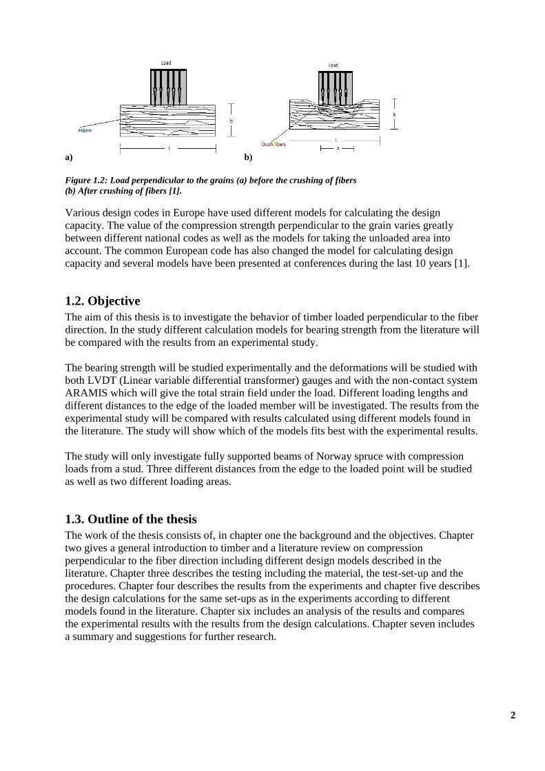
The design compression strength perpendicular to grain fc,90,d value is 2.5 N/mm2. And the

value of kc,90 should be calculated for the case with a concentrated load as follows. For a

member with a depth 2.5bh where a concentrated force with contact over the full width, b

of the member is applied to one face directly over a continuous or discrete support on the

opposite face, the factor kc,90 is given by:

0.5

ef

c,90,dl

l

250

l2.38-k

(2.9)

Where:

lef - is the effective length of bearing stresses, l is the contact length, h is the total depth of

specimen and b is the width of specimen.

Figure 2.6: Determination of effective lengths for a member with5.2

b

h

, (a) and (b) are continuous

support, [1]

The effective length for a load perpendicular to the grain shall be determined by a line with

the vertical inclination of 1:3.

The effective length of the load adjacent to the end of the member which is shown in Figure

2.6 (a) is.

10

3

hllef (2.10)

Where h is depth of member.

Where the distance a ≥ 2/3 h, from the edge of applied load to the end of member, Figure

2.6(b).

3

2hllef (2.11)

Where the h is depth of member, 40 mm or whichever is largest.

2.3.2. Eurocode 5 (EN 1995-1-1:2004) after amendment

Eurocode 5 was updated with an amendment for the calculation of compression strength

perpendicular to grain which was published 2009-05-20. In the new version of the standard

when a member is loaded perpendicular to the grain by a design load fc,90,d the expression for

compression stress σc,90,dwill be derived at the plane of contact between the load and the

member [2][1].

ef

c,90,d

c,90,dA

Fσ

(2.12)

Where:

Aef is the effective contact area perpendicular to the grain. “The effective area is obtained by

multiplying the contact zone width by an ‘effective contact length’. The effective contact

length can be the actual contact length, l , as indicated in Figure 2.6, or may be derived by

adding 30 mm to each end of the actual contact length but not more than “a" or ”l””,[10] as

shown in Figure 2.6.

The validation requirement will be:

c,90,dc,90c,90,d .fkσ (2.13)


efc,90,dc,90c,90,d .A.fkF (2.14)

The value of kc,90 should be taken to be 1, however for the bearing conditions which is shown

in Figure2.6 , when h21 l , where h is the depth of the member, a higher value can be used

for solid softwood and glued laminated timber as given in Table 2.1.The design compression

strength perpendicular to grain fc,90,d value is 2.5 N/mm2.

11

Table 2.1: Value of kc,90 for solid timber and glued laminated timber members subjected to compression

perpendicular to the grain [10]

Member support condition Solid softwood timber member

Continuous support kc,90 = 1.25

Discrete support kc,90 = 1.5

2.3.3. Italian code (CNR-DT-206:2006)

In the Italian code the unloaded length deals with in this certain way [2] [11].

Figure 2.7: Effective length, [2]

Where the expression shall be satisfied:

c,90,dc,90,d fσ (2.15)

ef

90,d

c,90,dlb

Fσ

(2.16)

efc,90,dc,90,d lbfF (2.17)

efl - is effective length given by considering the stress field distribution parallel to the grain

with an inclination of 1/3 and the limits shall be following:

hllef3

1

(2.18)

ll ef 2 (2.19)

The design compression strength perpendicular to grain fc,90,d value is 5 N/mm2 . However,

when it is allowed for the point of a maximum deformation perpendicular to grain it is

possible to use a value of 1.5 times the strength.

12

2.3.4. German Code (DIN 1052:2004)

In the German code the unloaded length is dealt with in the following way [2]:

Where the following expression shall be satisfied

1fk

σ

c,90,dc,90

c,90,d

(2.20)

And the compressive design stress is

ef

c,90,d

c,90,dA

Fσ

(2.21)


efc,90,dc,90,dc,90,d .A.fkF (2.22)

The symbols which are used:

efA -is the effective area under the load perpendicular to the grain.

c,90k -is the factor taking into account for unloaded length.

To calculate the effective area, efA , of the applied load in compression perpendicular to the

grain; it is possible to increase the length of the surface of the applied load along the direction

of grain up to 30 mm on both sides.[2]

The design compression strength perpendicular to grain fc,90,d value is 4.8 N/mm2. Principally

the German code is same as the new version of Euro-code and some of the values for kc,90 are

also equal. The value of kc,90 is possible to assume from 1 to 1.75 for distances according to

Figure 2.8 can be found in Table 2.2.

Figure 2.8: Effective length determination (a): continuous support (b): member with discrete support, [2]

13

Table 2.2: The value of the factor according to the germen code

Material c,90k

Glue-Laminated plain timber, hl 21 1.0

Plain timber with compressed tie , hl 21 1.25

Glue-Laminated timber with compressed tie and hl 21 ,

mml 400

1.5

Glue-Laminated timber and hl 21 , mml 400 1.75

2.3.5. Swedish new code (BKR: 2003)

According to the Swedish code the bearing strength can be calculated as follows [2] [12], the

resistance of timber member in compression perpendicular to grain is: AfκR c,90,dc,90c,90,d

(2.23)

Where:

c,90,dR - is the design value for compression perpendicular to the grain

dcf ,90 - is the design compressive strength of member

A - is the cross-sectional area of member

90,c - is the factor taking into account for the effected length according to Eurocode 5. In

practice normally kc,90 is not used and is therefore set to1.0.

2.3.6. Swedish old code

According to the Swedish old code the compression force perpendicular to the grain can be

calculated as follows [13], the resistance of timber member in compression perpendicular to

grain is:

c,90c,90c,90 fκσ (2.24)

lb

Fσ c,90

(2.25)

c,90c,90c,90,d .fκlbF (2.26)

Where,

c,90,dF - is the design value for compression perpendicular to the grain

c,90,df - is the design capacity for compression perpendicular to the grain

b - is the loaded area width

l - is the loaded area length

c,90 - is an increase factor which accounts for the unloaded length

14

c,90 =1 for cases A2, A3 and B2, B3

For cases A1 and B1 the value for κc,90 will calculate according to the following equation:

1,0

l

150

1,8

c,904

c4

150

l 150mm15for l (l=90)

l

l

l

150for

150mm15for

15mmfor

15

3. Description of material and methods

3.1. Description of tests

A series of tests was performed at Linnaeus University, Växjö laboratory on behalf of the

University in order to verify the compression strength perpendicular to grain of timber. The

experiments were divided into six different set-ups with two different loading areas and three

distances from the edge. The first series named A1, A2, A3 and the second named B1, B2, B3

as shown in Figure 3.1. All specimens have a dimension of (45 x 95 x500) mm. And the

compression tests were performed by applying a load on the specimens by using two steel

plates having contact area (45x95) mm or (90x95) mm, see Figure 3.1.

Figure 3.1: Schematic diagram for the series A1-A3 and B1-B3

3.2. Material

The material was 15 Norway spruce boards of strength class C24 with dimension (45 x95 x

4500) mm. The boards were all sawn with the annual rings more or less parallel with the face

side of the board. The boards were conditioned at a temperature of 21°C and a relative

humidity of 65% before the experiments. The dynamic modulus of elasticity of the boards

was measured using an MTG-grader before the tests. The boards were marked with a number

from 1 to 15 on one edge. Six 500 mm long sections were selected from each of the boards,

one for each loading case according to Figure 3.1. The selection were made so that the

specimens in the series A1and B1 were without knots in the central 300 mm and the

specimens in series A2, A3, B2 and B3 were without knots in 200 mm in one end. Of the 15

boards 11 boards were selected as giving specimens without knots in the right area, and these

selected boards were cut into six specimens. These six set-ups marked with board number and

specimen number, e.g. (1:A1 – 1:A3) and (1:B1 – 1:B3), see Figure 3.2.

16

4000

500

500

500

500

500

500

11:A1

1:A2

1:A3

1:B1

1:B2

1:B31

1

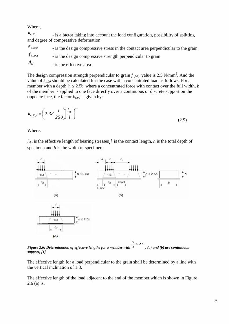
Figure 3.2: Specimen numbers marked on the board. Note: There should not be large knots on the

specimen’s compression area

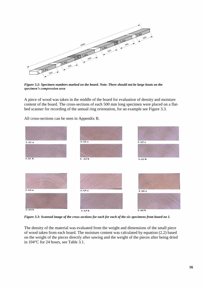
A piece of wood was taken in the middle of the board for evaluation of density and moisture

content of the board. The cross-sections of each 500 mm long specimen were placed on a flat-

bed scanner for recording of the annual ring orientation, for an example see Figure 3.3.

All cross-sections can be seen in Appendix B.

Figure 3.3: Scanned image of the cross-sections for each for each of the six specimens from board no 1.

The density of the material was evaluated from the weight and dimensions of the small piece

of wood taken from each board. The moisture content was calculated by equation (2.2) based

on the weight of the pieces directly after sawing and the weight of the pieces after being dried

in 104°C for 24 hours, see Table 3.1.

17

Table 3.1 Values of density and moisture content for boards.

Serial No. Board No. Density (kg/m3) Moisture content (MC in %)

1 1 395 11.96

2 2 490 12.40

3 3 428 11.67

4 4 366 10.78

5 5 503 12.09

6 6 436 10.91

7 9 402 12.78

8 10 377 11.52

9 11 405 11.81

10 14 482 15.87

11 15 415 11.09

Mean Density=412 Avg. MC= 12.1

3.3. Mechanical testing in the MTS machine

The mechanical tests were performed in an MTS 810 machine, which is a hydraulic one axial

loading machine with a capacity of 100 kN. The test specimens were mounted with the flat

side down on a steel beam, see Figure 3.4. The free end or both free ends were clamped to the

steel beam to avoid bending of the specimens. The load was applied with a steel stud with the

dimensions of (45 x 95) mm or (90 x 95) mm. The specimens were all placed with the pith

side down.

Figure 3.4: Material testing machine 810(MTS-810) with a specimen loaded in the center mounted on a steel

beam and clamped down in the ends.

18

The specimens were compressed with the steel studs at load rate of 1 mm/minute until the

deformation reached 3mm; the loading rate was thereafter increased to 3 mm/minute. The

loading was stopped when the total deformation was 10 mm. The load was registered by a

load cell placed between the machine and the steel stud and the deformation registered was

the movement of the steel stud (the piston in the machine). The load and deformation was

registered in a computer and later stored as excel files.

3.4. Strain field measurements

The ARAMIS (Optical 3D Deformation Analysis) was used to record the deformation during

the test. This system is based on two 4-mega pixel digital cameras,which take steroscopic

images during the test. The speciemen is sprayed with a speckle pattern that the ARAMIS

system is able to recognise between the images. By the speckle recognition system it is

possible to calculate the deformations and strains on a complete surface during loading. In

this case one set of specimens were recorded in all six load cases. The ARAMIS recorded the

deformations at each load step of 200 N. The data was used to calculate the strain field in x

and y direction.The ARAMIS system can be seen in Figure 3.5.

Figure 3.5.: ARAMIS setup with the speckle pattern painted on the specimen loaded close to the end with the

large steel stud. In the foreground the two cameras used for taking stereoscopic images of the specimen

during loading can be seen.

19

4. Results from the experiments

The compression perpendicular to grain test were performed as described in Chapter 2.2.1 and

evaluated according to EN 408:2010. [14] The experimental results are summarized in the

following three sub chapters.

4.1. Modulus of elasticity of the material

The longitudinal modulus of elasticitymean0,E can be calculated by the Equation 2.3, explained

in Chapter 2.1. [14]

0,meanE = 2 (f l)ρ 4 (4.1)

Where is density [kg/m3], f is frequency [Hz], l is length of the beam [m].

The modulus of elasticity perpendicular to grain 90,cE can be calculated using the following

equation

lbww

hFFE

12

12c,90

(4.2)

Where:

12 FF - is the increment of load on the linear portion of load deformation curve, in N.

12 ww - is the increment of deformation corresponding to 12 FF , in mm.

Figure 4.1 shows one of the curves from the experiments where the linear part of the curve,

the two points on line 1, is used to determine the Ec,90 and the line 2 used to determine the

c,90,maxF value.

20

Figure 4.1: Force-Deformation curve for the case 2- B1

The modulus of elasticity in the longitudinal direction and perpendicular to the grain direction

of the boards obtained from experimental investigation is presented in Table 4.1. This table

shows the average modulus of elasticity perpendicular to the grain for the six specimens from

each board. These six cases are from A1 to A3 and B1 to B3.

Table 4.1: Modulus of elasticity of boards

Serial No. Board No. Average Ec,90[MPa] E0,mean[MPa]

1 1 348 10092

2 2 436 13841

3 3 387 11926

4 4 377 9347

5 5 383 16401

6 6 346 12154

7 9 347 10833

8 10 335 11372

9 11 311 9987

10 14 369 15276

11 15 356 8817

Mean Ec,90 =363 Mean E0,mean = 11822

21

4.2. Compression force perpendicular to grain max,90,cF

The second part of the result includes the calculation of the values of maximum compression

force Fc,90,max shown in Table 4.2. The maximum compression force perpendicular to grain

Fc,90,max can be determined by using the definition according to EN 408 for block compression

as explained in the Chapter 2.2 by using the Figure 2.5.

Table 4.2: Compression force perpendicular to grain for each board and loading case

Board No.

Compression force perpendicular to grain Fc,90,max[kN]

A1 A2 A3 B1 B2 B3

1 23.80 20.44 18.88 40.63 39.28 32.32

2 30.67 27.35 24.59 52.71 44.87 38.60

3 23.66 22.43 22.08 40.54 38.18 33.89

4 24.66 20.52 18.10 37.51 33.99 28.53

5 22.70 19.92 18.52 40.04 35.14 30.42

6 25.70 22.37 19.07 41.23 36.90 32.84

9 21.66 19.04 16.21 35.00 29.99 27.74

10 22.03 20.92 17.82 36.93 42.68 30.77

11 22.32 20.49 18.63 38.02 33.22 30.98

14 26.16 23.35 21.76 44.03 41.17 34.42

15 24.66 20.56 18.57 38.25 31.47 32.84

The mean of the results for the compression force perpendicular to grain for each loading

configuration is presented in Table 4.3.

Table 4.3: Mean values of max bearing force

Serial No. Test

Name No.Of Test

Loaded

Length(mm)

Mean value of Max-

Compression Force max,90,cF( kN)

1 1A 11 45 24.36

2 2A 11 45 21.58

3 3A 11 45 19.48

4 1B 11 90 40.45

5 2B 11 90 36.99

6 3B 11 90 32.13

22

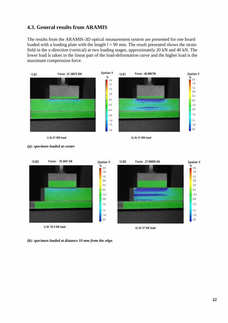
4.3. General results from ARAMIS

The results from the ARAMIS-3D optical measurement system are presented for one board

loaded with a loading plate with the length l = 90 mm. The result presented shows the strain

field in the y-direction (vertical) at two loading stages, approximately 20 kN and 40 kN. The

lower load is taken in the linear part of the load-deformation curve and the higher load is the

maximum compression force.

(a): specimen loaded at center

(b): specimen loaded at distance 10 mm from the edge.

23

(c): specimen loaded at the end

Figure 4.2(a - c): Effect of load on the specimen where the load at center, at distance 10 mm and at the end of

the member (specimen 12B1, 12B2 and 12B3 respectively)

Generally, from these images, it is observed that the stresses are concentrated in the region

below the loading contact area, see Figure 4.2. The maximum strain was in the range of -2 to

2 %. As shown in Figure 4.2 the tested set of specimen's series (load in the center of

specimen, specimen loaded at distance 10 mm and series loaded at the end) with constant

specimens size (l x b x h). However, within the subject boundaries, this visualization study is

not a complete study of strain and distribution of the bearing stresses of the specimens, but it

gives an impression of strain field and stress dispersion. All pictures are presented in

Appendix A.

24

5. Calculation according to different codes

In this chapter, the calculations of the maximum compression force perpendicular to grain

(Fc,90,d) according to the standards Euro-code 5 (EN1995-1-1:2004), old Euro-code, German

Code (DIN 1052:2004), Italian Code (CNR-DT 206:2006), Swedish Code (BKR: 2003) and

old Swedish code are presented. All codes were explained in chapter 2.3. And the design

compressive strength, fc,90d for all these codes are given in Table 5.1.

Table 5.1: Value of fc,90d for different codes

Strength

value

EU-5 before

amendment

EU-5 after

amendment

Italian

code

German

code

Swedish new code

‘BKR 2003’

Swedish code

‘old’

fc,90d

)/( 2mmN 2.5 2.5 5 4.8 7 7

Figure 5.1: Schematic diagram for test series

The calculation for compression force perpendicular to the grain according to different codes

as follows

25

5.1. Old version of Eurocode (EN 1995-1-1:2004) before amendment

The calculation of compression force perpendicular to the grain is: [2]

efdccdc AfkF ,90,90,,90, (5.1.1)

Where the factor kc,90, effective length lef, design compression strength perpendicular to grain

dcf ,90, and the effective area efA .The geometry of the specimen is described earlier and it can

be seen in Figure 3.1.However, the calculation of the setups will yield the following result.

Calculation for setup A1

With dimension b = 95mm, h = 45mm and the contact length l = 45mm as follows:

dcf ,90, =2.5 N/mm2

3

2hll ef = mm75

3

45245

(5.1.3)

5,0

90,250

38.2

l

llk

ef

c 84.245

75

250

4538.2

5,0

(5.1.4)

blA efef .

F c,90,dkc,90 f c,90,dAef 2.84 2.5 95 45 30.35kN

Calculation for setup B1

With dimension b = 95mm and h = 45mmand the contact length l = 90mm will be as follows:

mmh

ll ef 1203

45290

3

2

333.290

120

250

9038.2

25038.2

5,05,0

90,

l

llk

ef

c

blA efef .

F c,90,dkc,90 f c,90,dAef 2.333 2.5 95 90 49.87kN


With dimension b = 95mm, h = 45mm and the contact length l = 45mm are as follows:

mmh

ll ef 603

4545

3

54.245

60

250

4538.2

25038.2

5.05.0

90,

l

llk

ef

c

blA efef .

F c,90,dkc,90 f c,90,dAef 2.54 2.5 95 45 27.15kN

26


With dimension b = 95mm, h = 45mm and the contact length l = 90mm is as follows:

18.290

105

250

9038.2

25038.2

5.05.0

90,

l

llk

ef

c

mmh

ll ef 1053

4590

3

blA efef .

F c,90,dkc,90 f c,90,dAef 2.18 2.5 95 90 46.64kN

For setup A3 and B3 the calculation will be same as setup A2 and B2 respectively because of

the amplification factor kc,90 is the same.

5.2. New Eurocode 5(EN 1995-1-1:2004) after amendment

The calculation of compression force perpendicular to the grain according to the new version

of Eurocode 5 as follows: [2]

efdccdc AfkF ,90,90,,90, (5.2.1)

2,90, 5.2mm

Nf dc

Where the factor kc,90= cx , effective length lef, design compression strength perpendicular to

grain dcf ,90, and the effective area efA .

The geometry of the specimen is described earlier and it can be seen in Figure 3.1.


With dimension b = 95mm, h = 45mm and the contact length l = 45mm are as follows

dcf ,90, =2.5 N/mm2

25.1

9975)30245(95)302(

90

2

,dc,c

ef

kx

mmmmlbA

17.3199755.225.1,90,90,,90, efdccdc AfkF kN


With dimension b = 95mm and the contact length l = 45mm are as follows

dcf ,90, =2.5 N/mm2

25.1

14250)30290(95)302( 2

c

ef

x

mmmmlbA

27

kNAfkF efdccdc 53.441425005.225.1,90,90,,90,

Calculations for setup A2

With dimension b = 95mm, and the contact length l = 45mm are as follows

dcf ,90,=2.5 N/mm

2

25.1

8075)103045.(95)1030( 2

c

ef

x

m mm mm mlbA

kNAfkF efdccdc 23.2580755.225.1,90,90,,90,

Calculations for setup B2


dcf ,90, =2.5 N/mm2

25.1

12350)103090(95)1030( 2

c

ef

x

m mm mm mlbA

efdccdc AfkF ,90,90,,90,kN60.38123505.225.1



dcf ,90, =2.5 N/mm2

25.1

7125)3045(95)30( 2

c

ef

x

m mm mlbA

efdccdc AfkF ,90,90,,90, kN27.2271255.225.1



dcf ,90, =2.5 N/mm2

25.1

11400)3090(95)30( 2

c

ef

x

m mm mlbA

efdccdc AfkF ,90,90,,90, kN63.35114005.225.1

28

5.3. Italian code (CNR-DT 206-2006)

The calculation of compression force perpendicular to the grain according to Italian code as

follows: [2]

efdcdc AfF ,90,,90,

=5 N/

Where the factor kc,90,d , effective length lef, design compression strength perpendicular to

grain dcf ,90,

and the effective area efA .




=5 N/

kNlbfF efdcdc 63.3575955,90,,90,



=5 N/

kNlbfF efdcdc 25.3370955,90,,90,



=5 N/

kNlbfF efdcdc 50.2860955,90,,90,



=5 N/

dcf ,90,

2mm

dcf ,90,

2mm

mmhlll ef 7575,90min32;2min

dcf ,90,

2mm

mmhlll ef 7070,90min103

1,2min

dcf ,90,

2mm


1;2min

dcf ,90,

2mm

29

kNlbfF efdcdc 25.71150955,90,,90,



=5 N/

kNlbfF efdcdc 50.66140955,90,,90,



=5 N/

kNlbfF efdcdc 00.57120955,90,,90,

5.4. German code (DIN 1052:2004)

The calculation of compression force perpendicular to the grain according to German code as

follows: [2]

=4.8 N/

1. ,90,90,

,90,

dcc

dc

fk

ef

dc

dcA

F ,90,

,90,

And,

efdccdc AfkF ,90,90,,90,

25.190, ck

Where the factor kc,90,d , effective length lef, design compression strength perpendicular to


The geometry of the specimen is described earlier and it can be seen in Figure 3.1


dcf ,90,

2mm


1,2min

dcf ,90,

2mm


1;2min

dcf ,90,

2mm

30



efdccdc lbfkF ,90,90,,90, .

kNF dc 75.4275.95.8.4.25.1,90,




kNF dc 9.3970958.425.1,90,




kNF dc 2.3460958.425.1,90,




kNF dc 5.85150958.425.1,90,




kNF dc 8.79140958.425.1,90,



1,2min


1;2min



1,2min

31




kNF dc 4.68120.95.8.4.25.1,90,

5.5. Swedish new code (BKR: 2003)

The calculation of compression force perpendicular to the grain according to the new Swedish

code as follows: [2]

AfkR dccdc ,90,90,,90,

A

FR

dc

dc

,90,

,90,

AfkF dccdc ,90,90,,90,

dcf ,90, = 7 N/mm2

Where the factor, kc,90 , effective length, lef, design compression strength perpendicular to





kNAfkF dccdc 92.29459571,90,90,,90,



kNAfkF dccdc 85.59909571,90,90,,90,

Calculations for setups A2 and A3.


kNAfkF dccdc 92.29459571,90,90,,90,


1;2min

32

Calculations for setups B2 and B3


kNAfkF dccdc 85.59909571,90,90,,90,

5.6. Swedish old code

The calculation of compression force perpendicular to the grain according to the Swedish old

code as follows: [13]

90,90, ccc f

hb

Fc

90,

90,,90, ccdc fhbF

2

90, /7 mmNf c

Where the factor is c , design compression strength perpendicular to grain dcf ,90,, width of

specimen b, contact length, h.



With dimension b = 95mm and h = 45mm l = 90 mm will be as follows:

1,0

l

150

1,8

c,904

c4

150

l 150mm15for l (l=90)

c =1.136

kNfhbF ccdc 00.347136,1459590,,90,

Calculations for setup A2 and A3

With dimension b = 95mm and h = 45mm will be as follows:

14,190

1504

l

l

l

150for

150mm15for

15mmfor

33

c 1

kNfhbF ccdc 93.2971459590,,90,


With dimension b = 95mm and h = 90mm l= 90 mm will be as follows:

1,0

l

150

1,8

c,904

c4

150

l 150mm15for l (l=90)

90

1504ck = 1.136

kNfhbF ccdc 00.687136,1909590,,90,

Calculations for setup B2 and B3

With dimension b = 95mm and h = 90mmwill be as follows:

c 1

kNfhbF ccdc 85.5971909590,,90,

All calculated values for the maximum compression force perpendicular to grain ( )

according to the different codes which are present in Table 5.3.

Table 5.3: Compression force (Fc,90,d) according to different codes

Specimen

no.

EU5

Old(kN)

EU 5

New(kN)

Italian

(kN)

German

(kN)

Swedish

New(kN)

Swedish

Old(kN)

30.35 31.17 35.62 42.75 29.92 34.00

27.15 25.23 33.25 39.90 29.92 29.93

27.15 22.27 28.50 34.20 29.92 29.93

49.87 44.53 71.25 85.51 59.85 68.00

46.64 38.60 66.50 79.82 59.85 59.85

46.64 35.63 57.00 68.40 59.85 59.85

The codes or models are explained in chapter 2.3. And all calculations are presented in appendix A.

dc,90,F

1A

2A

3A

1B

2B

3B

(*)

l

l

l

150for

150mm15for

15mmfor

34

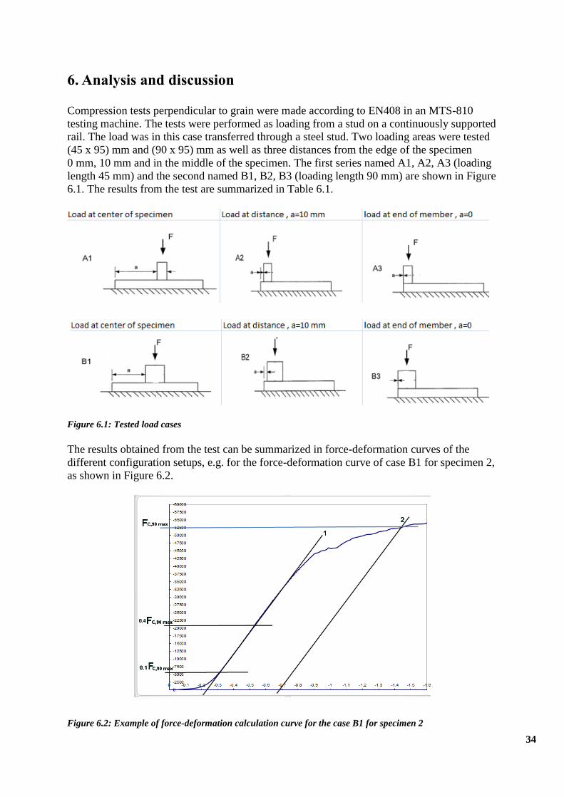
6. Analysis and discussion

Compression tests perpendicular to grain were made according to EN408 in an MTS-810

testing machine. The tests were performed as loading from a stud on a continuously supported

rail. The load was in this case transferred through a steel stud. Two loading areas were tested

(45 x 95) mm and (90 x 95) mm as well as three distances from the edge of the specimen

0 mm, 10 mm and in the middle of the specimen. The first series named A1, A2, A3 (loading

length 45 mm) and the second named B1, B2, B3 (loading length 90 mm) are shown in Figure

6.1. The results from the test are summarized in Table 6.1.

Figure 6.1: Tested load cases

The results obtained from the test can be summarized in force-deformation curves of the

different configuration setups, e.g. for the force-deformation curve of case B1 for specimen 2,

as shown in Figure 6.2.

Figure 6.2: Example of force-deformation calculation curve for the case B1 for specimen 2

35

Figure 6.3 shows the resulting force-deformation curve for all six types (A1-3 and B1-3) for

specimen number 1. The curves shows that for setup B with a longer loading length the

maximum capacity is larger than for setup A with a smaller loading length.

Figure 6.3: A general graphical representation for maximum force and deformation

Moreover the results obtained from the test have shown that the compression perpendicular to

grain strength of the beam when loaded is dependent on the loading situation and the loading

area. The compression capacity is about 65-70% higher for the case with a doubled loading

area. There is also an effect of the distance from the end of the rail. Loading in the middle of

the long specimen increased the capacity with approximately 25%. Moving the loading point

only 10 mm from the edge increased the capacity by 10% compared to loading at the edge,

see Table 6.1.

Several researchers, e.g. Van der put et al. [7], Madsen [8], Blass and Görlacher[9], as well as

several codes have proposed that the design should be based on an assumption of an effective

length l ef due to the load spread in the material. For example see Eurocode (Chapter 2.3.1)

where the load spread is assumed to be 1:3. The ARAMIS-3D optical measurement images as

shown in Figure 6.4, (compression at center, at distance 10 mm and at the edge) with constant

specimens’ size (90x 95), it is observed that the stresses are concentrated in the region below

the loading contact area. The load spread in these images seems to be steeper than 1:3. This

might be due to the sharp edges of the steel stud used to transfer the load. Especially the load

close to the edge seems to have a load spread that is very small and a very limited area outside

the directly loaded area is affected by strains.

36

Figure 6.4(a - c): Deformation under compression, effect of load on the specimen where the load at center, at

distance 10 mm and at the end of the member (specimen 12B1, 12B2 and 12B3 respectively) [15]

The capacity of the compression force was calculated according to six different codes. The

codes were two versions of Eurocode 5, the Italian code (CNR-DT 206-2006), the German

code (DIN 1052:2004) and two versions of the Swedish code. As shown in Table 6.1 below it

is easy to see that the different codes will lead to different maximum compression force even

when the test material was the same. In general the highest compression stress value was the

B1 case which has the biggest loading area (90x95) and the largest effective length. The

effective length will be increase in both directions of the loaded area for this case. The

opposite case was A3 which has the smallest loading area (45x95) and the smallest effective

length, because of the edge load position, where the effective length can be included in one

direction only. The effect of increasing the effective length in only one direction compared to

the two other cases (load in the middle and load from 10 mm from the edge) will lead to a

lower maximum compression force.

37

Table 6.1: Comparison of test results of Max Compression Force with different codes

Specimen

no.

Test

Data

EU5

Old(kN)

EU 5

New(kN)

Italian

(kN)

German

(kN)

Swedish

New(kN)

Swedish

Old(kN)

24.36 30.35 31.17 35.62 42.75 29.92 34.00

21.58 27.15 25.23 33.25 39.9 29.92 29.93

19.49 27.15 22.27 28.50 34.2 29.92 29.93

40.45 49.87 44.53 71.25 85.5 59.85 68.00

36.99 46.64 38.60 66.50 79.8 59.85 59.85

32.13 46.64 35.63 57.00 68.4 59.85 59.85

Comparing the results from the different calculations according to the codes it is possible to

see that calculations according to the new Eurocode 5 resulted in the lowest maximum

compression force. The results also showed that the effect of load area is taken into account in

all the codes. For the Eurocode the compression force is approximately 1.5 times higher for

the bigger load area while for many of the older national codes the maximum is almost

doubled for the bigger load area. Several of the codes also show an effect of load spread. The

value for loading in the middle of the specimen, with the load spreading in two directions, is

higher than loading at the edge.

The results also showed that in all cases the experimental results were lower than the capacity

calculated according to the codes. Moreover the code that gave results closest to the

experimental results was the new version of Eurocode 5. The results from the code showed

results that were 10-25% higher than the results from the experiments.

The results also show that Eurocode is farther from the experimental results for the 45 mm

wide specimens than for the 90 mm wide specimens. But the results from Eurocode show a

result that is approximately 25% higher for loading in the middle of the specimen than at the

edge, which agrees well with the experimental results. The effect of loading 10 mm from the

edge is also approximately 10% higher than loading at the edge which also agrees well with

the code. This shows that Eurocode at least takes the loading area and distance from the edge

into account in a reasonable way at least when compared with these tests

However, the compression stress perpendicular to grain in new Eurocode 5 are higher than the

test data and that happen because of some reasons such as

1) Using a steel stud with sharp edges. Steel stud is a much harsher condition than using

a wood stud.

2) The specimens were not knot free 100% and that will surely affect the test results.

1A

2A

3A

1B

2B

3B

38

7. Conclusion

Based on a literature review and from the specimens tested in this study, it can be concluded

that the compression perpendicular to the grain in timber is an important property for

structural design. It is dependent on the loading situation, the loading area and the type of

specimen. The case studied in this case is the loading from a stud on a continuously supported

rail. In this thesis especially the effect of loading area and loading position was investigated.

Two loading areas were tested (45x 95) mm and (90 x 95) mm as well as three distances from

the end of the specimen 0 mm, 10 mm and in the middle of a long specimen.

The results show that there is a great influence of loading area. The compression capacity is

about 65-70% higher for the case with a doubled loading area. There is also an effect of the

distance from the end of the rail. Loading in the middle of the long specimen increased the

capacity with approximately 25%. Moving the loading point only 10 mm from the edge

increased the capacity by 10% compared to loading at the edge.

The capacity of the compression force was calculated according to six different codes. The

codes were two versions of Eurocode 5, the Italian code (CNR-DT 206-2006), the German

code (DIN 1052:2004) and two versions of the Swedish code (BKR). The results showed that

in all cases the experimental results were lower than the capacity calculated according to the

code. The main explanation to this is probably that the loading was done with a steel stud with

relatively sharp edges. Compared to a timber stud this loading is much harder.

The code that gave results closest to the experimental results was the new version of

Eurocode 5. The results from the code showed results that were 10-25% higher than the

results from the experiments. The results also show that Eurocode is farther from the

experimental results for the 45 mm wide specimens than for the 90 mm wide specimens.

The results from Eurocode show a result that is approximately 25% higher for loading in the

middle of the specimen than at the edge, which agrees well with the experimental results. The

effect of loading 10 mm from the edge is also approximately 10% higher than loading at the

edge which also agrees well with the code. This shows that Eurocode at least takes the

loading area and distance from the edge into account in a reasonable way at least when

compared with these tests.

The experimental results still show to low strength compared to the codes. A further study

using another material in the loading stud should be done. This could show how much of the

low strength is due to the rather hard loading conditions in this study.

39

8. References

[1] Porteous, J. and Kermani, A.2007: “Structural timber design to Eurocode 5” Blackwell

Science Ltd, 9600 Garsington Road, Oxford OX4 2DQ, UK.

[2] Formolo, F. and Granström, R. 2007: “Compression perpendicular to grain and

reinforcement of a pre-stressed timber deck”. Chalmers Master Thesis 2007:25 Department of

Division of Structural Engineering, Steel and Timber Structures, Chalmers University of

Technology SE-412 96 Göteborg Sweden,

[3] Image from google search, “http://limited-vision-stock.deviantart.com/art/Wood-Texture-

03-197276178”Web. June 2014

[4] Crocetti, R., Johansson, M., Johansson, J.et al.2011: “Design of timber structures”

Exaktprinting I Malmo AB, Swedish Wood, P.O.Box 55525 SE 102 04 Stockholm Sweden.

[5] EN 1991-1-1:2002. Eurocode 1: Actions on Structures. Part 1-1: General

Actions – Densities, Self-Weight and Imposed Loads for Buildings, CEN, European

Committee for standardization.

[6] Thelandersson S. and Mårtensson A 2012:, "Design Principles for Timber in Compression

Perpendicular to Grain" Proceedings of the CIB-W-18, Paper -30-20-1. Meeting Forty-Five

Forty-Five Vaxjo Sweden, August 2012.

[7] Blass, H.-J.; Görlacher, R. 2004: “Compression perpendicular to the grain“, Proceedings

of the 8thWorld Conference on Timber Engineering, Vol. II, Lahti, Finland, 2004

[8] van der PutT.A.C.M. 1982: A general failure criterion for wood, Proc. IUFRO S5.02

paper 23, 1982, Boras, Sweden.

[9] EN 1193:1998. Timber Structures – Structural Timber and Glued Laminated

Timber – Determination of Shear Strength and Mechanical Properties Perpendicular to the

Grain, CEN, European Committee for standardization.

[10] EN-1-1:2004: Eurocode 5: Design of timber structures. Part 1-1: General – common

rules and rules of buildings, CEN, European Committee for standardization

[11] CNR-DT 206 2006: Istruzioni per il Progetto, l´Esecuzione e ilCollaudodelleStrutture di

legno, ConsiglioNazionaledelleRicerche, Roma, Italy

[12] BKR: 2003 2003:, Design regulations BKR. Boverket, BFS 1998:39

[13] Building and Design Regulations, BFS 1993:58 with amendments up to BFS 1998:39,

BFS 1999:7 and BFS 1999:46, Swedish Board of Housing, Building and Planning

Month of publication: June 2000.

[14] BS EN 408:2010, Timber structures: Structural timber and glued laminated timber.

40

[15] Larsen, H.J.,Leijten,A.J.M., Van der Put, T.A.C.M. 2011: “The design rules in Eurocode

5 for compression perpendicular to the grain – Continuous supported beams.” CIB-W18:

Timber Structure 1-43, Danish Timber Information 2011.

41

Appendix A: ARAMIS Images

The following images which were taken by ARAMIS are general view of the effect on wood

structures at the maximum force.

Figure 9.1- ARAMIS test result A1

Figure 9.2 - ARAMIS test result A2

Figure 9.3 - ARAMIS test result A3

42

Figure 9.4- ARAMIS test result B2

Figure 9.5 - ARAMIS test result B3

43

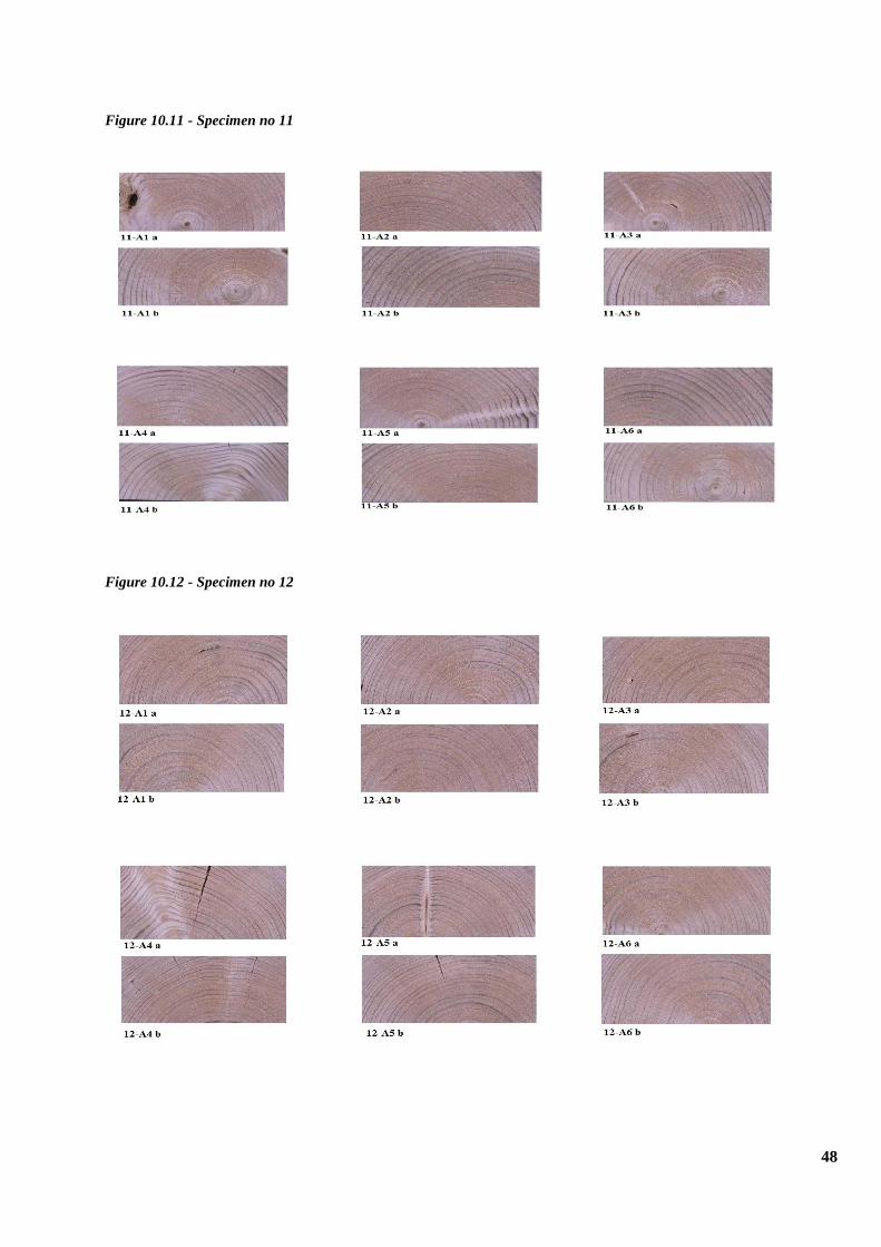
Appendix B: Cross-sectional view of specimens

Following pictures below are tested board´s specimens’ cross-sectional area which shows the

grains direction.

Figure 10.1 - Specimen no 1

Figure 10.2- Specimen no 2

44



45



46



47



48



49



50


51

Appendix C: Force and deformation diagram

The following figures below are general expression for each board’s combine graph for

different series.

Figure 11.1a - Specimen no 1A

Figure 11.1B - Specimen no 1B

52

Figure 11.3A - Specimen no 3A


53



54



55



56



57

Appendix D: Force-deformations graphs MTS 810

The following figures below are general expression for each board’s single graph for different

series in MTS 810.

Figure 12.1 Force-deformation for different loading situations.2A1, 2A2 and 2A3

-80000

-70000

-60000

-50000

-40000

-30000

-20000

-10000

0

10000

-11 -10 -9 -8 -7 -6 -5 -4 -3 -2 -1 0

MTS

81

0 F

orc

e(N

)

MTS 810 Displcement (mm)

Specimen 2-A1

-60000

-50000

-40000

-30000

-20000

-10000

0

10000

-12 -10 -8 -6 -4 -2 0 2

MTS

81

0 F

orc

e(N

)

MTS 810 Displacement (mm)

Specimen 2-A2

-50000

-40000

-30000

-20000

-10000

0

10000

-15 -10 -5 0

MTS

81

0 (

N)


Specimen 2-A3

58

Figure 12.2 Force-deformation for different loading situations.2B1, 2B2 and 2B3

-110000

-90000

-70000

-50000

-30000

-10000

10000

-12 -10 -8 -6 -4 -2 0

MTS

81

0 F

orc

e (

N)


Specimen 2-B1

-80000

-70000

-60000

-50000

-40000

-30000

-20000

-10000

0

10000

-15 -10 -5 0

MTS

81

0 F

orc

e (

N)


Specimen 2-B2

-70000

-60000

-50000

-40000

-30000

-20000

-10000

0

10000

-15 -10 -5 0

MTS

81

0 F

orc

e (

N)


Specimen 2-A3

59

Documents

Compression perpendicular to grain in timber - …733343/FULLTEXT01.pdf · Compression perpendicular to grain in timber ... When the wood material is subjected to a compression load