COMPRESSION AND RADIATION OF HIGH-POWER SHORT RF PULSES. I. ENERGY

Progress In Electromagnetics Research, Vol. 116, 239–270, 2011

COMPRESSION AND RADIATION OF HIGH-POWERSHORT RF PULSES. I. ENERGY ACCUMULATION INDIRECT-FLOW WAVEGUIDE COMPRESSORS

K. Sirenko

King Abdullah University of Science and Technology (KAUST)4700 KAUST, Thuwal, 23955-6900, Saudi Arabia

V. Pazynin and Y. Sirenko

Institute of Radiophysics and ElectronicsNational Academy of Sciences of Ukraine (IRE NASU)12 Acad. Proskura Str., Kharkiv, 61085, Ukraine

H. Bagcı

King Abdullah University of Science and Technology (KAUST)4700 KAUST, Thuwal, 23955-6900, Saudi Arabia

Abstract—Proper design of efficient microwave energy compressorsrequires precise understanding of the physics pertinent to energyaccumulation and exhaust processes in resonant waveguide cavities.In this paper, practically for the first time these highly non-monotonictransient processes are studied in detail using a rigorous time-domainapproach. Additionally, influence of the geometrical design andexcitation parameters on the compressor’s performance is quantifiedin detail.

1. INTRODUCTION

A microwave (energy) compressor is a device capable of convertinga long-duration low-amplitude input pulse into a short-durationhigh-amplitude output pulse. Active compressors achieve this byaccumulating the energy of input pulse for a relatively long periodof time and then exhausting the accumulated energy in the form ofa short high-power output. Efficient microwave pulse compression is

Received 20 February 2011, Accepted 26 April 2011, Scheduled 4 May 2011Corresponding author: Kostyantyn Sirenko ([email protected]).

240 Sirenko et al.

needed in several fields of science and engineering: Compressors areused as components of particle accelerators [1, 2] and radars [3], andutilized in data transmission [4], energy transfer [5], plasma heating [6],and biological studies [7].

An active microwave compressor consists of a storage unit, whichacts as an energy accumulator, and a switch, which terminates theenergy accumulation in the storage unit and lets the accumulatedenergy exhaust [8]. Although the storage unit might be designed ina number of ways, the most common designs utilize high-Q waveguidecavities [1, 2, 9–14]. As for switches, a few design options exist:switches that change the resonance condition of the whole devicevia discharge [9, 14] or controlled effects in semiconductors [12, 15],distributed-grating type switches [16], interference plasma (gasdischarge) switches [10, 13], trigatron commutators [11, 14], andresonant switches [17, 18]. Apparently, a compressor is a resonantdevice; its design and analysis require a detailed study of long-duration accumulation and short-duration exhaust processes involvingweakly-decaying fields of quasi-monochromatic pulses. For properoperation of the compressor, the design parameters of the storageunit and the switch, and the input pulse parameters shouldbe correctly fitted and completely consistent. A miscalculatedvariation in any of these parameters usually causes an avalanche ofchanges, which can dramatically reduce the compressor’s performance.Unfortunately, the effect of these variations cannot be predicted usingsimplified and approximate mathematical models, which separatelyaccount for characteristics of compressor’s isolated components.For example, design and characterization methods, which employapproximate mathematical models [1, 8, 9, 12] and experimental testingprocedures [2, 14], do not take into account the time-dependentfeatures of the compressors. Moreover, they require tuning of thecompressors’ design parameters manually [1, 2, 12, 14]. To this end,mathematically rigorous and accurate full-wave simulators, whichmodel the compressor as a whole and throughout the entire duration oftime-dependent energy accumulation and exhaust, should be utilizedin design and analysis of compressors.

Time-domain methods are best suited for this job mostly becausethey allow real-time observation of all wave interactions taking placeduring the energy accumulation and exhaust. However, very longobservation times required to study the transient resonant processesenforce two main constraints on the time-domain method used:(i) High accuracy to avoid error build up during long simulationtimes and to obtain reliable results; (ii) high efficiency to completethe simulations using reasonable computational resources. In this

Progress In Electromagnetics Research, Vol. 116, 2011 241

work, finite-difference time-domain (FDTD) method described in [19]is preferred for this purpose. This simulator achieves high accuracyby employing mathematically exact absorbing boundary conditions(EACs) [19–21]. Its efficiency is increased via the use of a numericallyexact blocked-FFT based scheme, which reduces the computationalcost of temporal convolutions present in the non-local EACs [19, 22–28].Combination of these two advanced computational techniques rendersthis FDTD simulator an ideal candidate for accurately analyzing theenergy accumulation and exhaust in compressors.

It is not possible to design a properly functioning energy compres-sor without in-depth understanding of the energy accumulation pro-cess. The energy accumulation process, which involves formation ofhighly resonant high-power pulses in the storage unit, is non-uniformin time; hence, a real-time study is required to fully understand allpertinent physical phenomena. In this work, practically for the firsttime, all processes inside a compressor are studied in time-domain indetail from the very beginning of the excitation right until the end ofthe accumulated energy’s exhaust. Moreover, the influence of variousparameters of the compressor and the excitation on the energy accu-mulation process and, thus, the overall compressor’s performance, isdiscussed. As an example, the paper analyzes in detail the energy accu-mulation processes in a rectangular direct-flow waveguide compressorexcited by TE0,n waves, which is designed following the scheme out-lined in [17]. This paper supplements [17]; together they allow forrigorously formulating and efficiently solving the problem of designingand analyzing various compressors in VHF, UHF, SHF and EHF bands(from 300 MHz to 300GHz).

The novel contributions of this work are twofold: (i) It presents arigorous scheme to design and characterize energy compressors, whichallows to study a compressor as a whole in contrast to the existingdesign frameworks, which separately account for characteristics of thecompressor’s isolated components. The proposed method is capableof performing a fully rigorous characterization of the time-dependentenergy accumulation and exhaust processes. (ii) A detailed discussionon the effects of the various design parameters (geometric dimension,switching, etc.) and the durations of the excitation and energyaccumulation and exhaust processes on the efficiency of the compressoris presented.

The remainder of this paper is organized as follows. Section 2starts with a description of the mathematical model, and thenintroduces several time- and frequency-domain characteristics used inthe design and analysis of the compressors. Section 3 starts with abrief summary of the design scheme used, and then presents a detailed

242 Sirenko et al.

discussion of the energy accumulation processes and explains howvarious parameters of the compressors and the excitation influence thecompressor’s performance. Section 4 provides a short description ofthe FDTD simulator with FFT-accelerated EACs. Section 5 presentsconclusions and future research avenues.

2. MATHEMATICAL MODEL ANDCHARACTERISTICS OF MICROWAVE COMPRESSORS

This section first introduces the mathematical model (Section 2.1),and then describes the compressor’s time- and frequency-domaincharacteristics in terms of model parameters (Sections 2.2 and 2.3).It should be noted here that the mathematical model parameters andthe time and frequency domain characteristics are extensively referredto in Section 3, where the energy accumulation process is discussed indetail.

2.1. Mathematical Model

Consider the two-dimensional (2-D) model of the rectangular direct-flow waveguide compressor presented in Fig. 1. TE0,n wave interactionson this structure are mathematically modelled by the following initial-boundary value problem [20, 21]:

[−εr (g) ∂2t −P +∂2

z + ∂2y

]U (g, t) = 0; t > 0, g = {y, z} ∈ Q

U (g, 0) = 0, ∂tU (g, t)|t=0 = 0; g ∈ QL

Etg (g, t)|g∈S = 0; t ≥ 0(1)

Here, {x, y, z} are Cartesian coordinates; P [U ] = ∂t[Z0σ0(g, t)U(g, t)];U = Ex, Ey = Ez = Hx = 0; ~E (g, t) = {Ex, Ey, Ez} and~H (g, t) = {Hx,Hy,Hz} are the vectors of electric and magneticfields; S represents the perfect electrically conducting (PEC) sur-faces of the compressor; Etg (g, t) is the component of electric fieldthat is tangential to S; Q = QL ∪ I ∪ II ∪ L1 ∪ L2 is thephysical domain; QL = {g = {y, z} ∈ Q : −L1 < z < L2} is thecomputation domain; σ0 (g, t) and εr (g) represent the conductiv-ity and the relative permittivity; Z0 = (µ0/ε0)

1/2, ε0 and µ0

are the wave impedance, permittivity and permeability of the freespace, respectively. σ0 (g, t) and εr (g) are piecewise constant func-tions in space, and the conductivity’s time dependence is utilizedto change the compressor’s mode of operation (energy accumula-tion/exhaust). Domains I = {g ∈ Q : −a1/2 ≤ y ≤ a1/2, z < −L1},


2

z L=

1

z L= −

h

a

0 l

1

L1

a 2

a 2

L z

LQ

1

d 2

d 3

d

y

coupling window

(beyond-cutoff diaphragm)

storage unit switch

II I

Sfeeding waveguide output waveguide

d

Figure 1. Geometry of a direct-flow compressor on the basis ofrectangular waveguides.

and II = {g ∈ Q : −a2/2 ≤ y ≤ a2/2, z > L2} represent infinite reg-ular input (feeding) and output waveguides, and contours L1 ={g ∈ Q : z = −L1} and L2 = {g ∈ Q : z = L2} represent virtualboundaries between I and II and the computation domain QL, respec-tively. The physical domain Q is unbounded in the z (longitudinal)direction. In this model, the SI system is used for all physical quan-tities except the time t, which is multiplied with the speed of light infree space and measured in meters.

Let U i (g, t) represent an incident pulse (excitation), which arrivesfrom the feeding waveguide I upon the virtual boundary L1 at timet > 0. The total field U (g, t) in I can be represented as a sum ofincident and scattered fields: U (g, t) = U i (g, t) + U s

1 (g, t), g ∈ I; inII total field consists of only the scattered field: U (g, t) = U s

2 (g, t),g ∈ II. U i (g, t), U s

1 (g, t), and U s2 (g, t) are represented in terms of

modes via separation of variables [20, 21]:

U i (g, t) =∑

n

vn,1 (z, t) µn,1 (y); g ∈ I,

U sj (g, t) =

∑n

un,j (z, t) µn,j (y); g ∈ I for j = 1,

g ∈ II for j = 2, j = 1, 2.

(2)

The spatio-temporal (mode) amplitudes vn,1 (z, t) and un,j (z, t) and

244 Sirenko et al.

the transverse functions µn,j (y) are related by

{vn,1 (z, t)un,j (z, t)

}=

aj/2∫

−aj/2

{U i (g, t)U s

j (g, t)

}µn,j (y) dy; g ∈ I for j = 1,

g ∈ II for j = 2, j = 1, 2.

where aj represent the widths of the waveguides I (j = 1) andII (j = 2) (Fig. 1). It should be noted that vn,1 (z, t), un,j (z, t)and µn,j (y) define a complete set of modes for representing thewaves U i (g, t) and U s

j (g, t). The transverse functions µn,j (y) and thecorresponding eigenvalues λn,j are known; for the TE0,n waves in 2-Dwaveguides considered here, they are given by [20, 21]:

µn,j (y) =

√2aj

sin(nπ

y+aj/2aj

), λn,j =

nπ

aj; n = 1, 2, 3..., j = 1, 2.

The unbounded (open) problem (1) in the domain Q can beconverted into a bounded (closed) one in the domain QL, which ismore suitable for numerical solution, by introducing EACs on thevirtual boundaries L1 and L2 (Fig. 1). In this work, the EACs derivedin [20, 21] are used. It should be noted here that enforcing EACs onvirtual boundaries results in mathematically exact conversion of theunbounded problem to the bounded one [20, 21]. The EACs on L1 andL2 are [20, 21]:

U (y,−L1, t)− U i (y,−L1, t) =∑

n

t∫

0

J0 (λn,1 (t−τ))

×

a1/2∫

−a1/2

∂z

[U (y, z, τ)−U i (y, z, τ)

]∣∣z=−L1

µn,1 (y) dy

dτ

µn,1 (y) ;

−a1

2≤ y ≤ a1

2, t ≥ 0,

U (y, L2, t) = −∑

n

t∫

0

J0(λn,2 (t−τ))

×

a2/2∫

−a2/2

∂zU (y, z, τ)|z=L2µn,2 (y) dy

dτ

µn,2 (y) ;−a2

2≤y≤ a2

2, t≥0.


Here, J0 (.) represents the Bessel function of the zeroth order. It shouldbe noted here that these EACs are nonlocal both in space and time(note the ranges of integrals over τ and y); their direct numericalimplementation results in increased computational requirements. Thiscan be alleviated by using localization techniques [20, 21] or byaccelerating the computation of temporal convolutions via the use ofblocked FFTs [22–28] as described in [19]. It should be noted herethat both of these techniques are exact, i.e., their application does notintroduce additional errors into the numerical solution.

2.2. Time-domain Characteristics

Four different characteristics are defined in the time-domain to quantifythe energy accumulation and exhaust processes on compressors:(i) Energy Efficiency is the ratio of the useful output energy to the

total input energy:

η =W s

2 (t3; t4)W i

1 (t1; t2). (3)

Here, W i1 (t1; t2) and W s

2 (t3; t4) represent the total energies fedinto compressor from the waveguide I between times t1 and t2,and transmitted into the output waveguide II between times t3and t4, respectively; t1 and t2 are the turn-on and off times of theexcitation (t1 is usually zero), the useful output pulse is non-zerobetween t3 and t4. W i

1 (t1; t2) and W s2 (t3; t4) are computed using:

Wi(s)j (t1; t2) = − (+)

∫ t2

t1

Pi(s)j (t)dt; j = 1, 2, (4)

where −P i1 (t) and P s

2 (t) represent the instantaneous powerentering and leaving the computation domain QL through thevirtual boundaries L1 and L2, respectively and are computedby [32]:

Pi(s)j (t) =

∫

Lj

([~E

i(s)j (g, t)× ~H

i(s)j (g, t)

]· ~nj

)dS

=

−a1/2∫−a1/2

[E

i(s)x (y,−L1, t)H

i(s)y (y,−L1, t)

]dy for j =1, g ∈ L1

a2/2∫−a2/2

[Es

x (y, L2, t) Hsy (y, L2, t)

]dy for j =2, g ∈ L2

(5)

where ~nj represents the unit normal defined on the boundary Lj

which points outwards from the domain QL, and ~Ei(s)j (g, t) and

246 Sirenko et al.

~Hi(s)j (g, t), g ∈ Lj , are the boundary values of incident (scattered)

electric and magnetic fields.η is a positive number less than or equal to one, — obviously, thecloser η to one, the more efficient compressor is.

(ii) Degree of Compression quantifies how short the useful outputpulse is in comparison to the input pulse — it is defined as theratio of input and output pulse durations:

β =T i

T s2

, (6)

where T i = t2 − t1 and T s2 = t4 − t3 are the durations of input

and output pulses, respectively. Normally, β is a positive numbergreater than one – obviously, larger β means higher compressionrate.

(iii) Power Gain is a measure of compressor’s ability to increase thepower of the output pulse in comparison to the input pulse. Powergain is defined as the product of the degree of compression (6) andthe energy efficiency (3):

θ = β · η (7)

It is clear from (7) that θ is the ratio of the mean powers of theinput and output pulses. θ is a positive number greater than one— obviously, larger θ means higher power gain.

(iv) Instantaneous Energy Accumulation Efficiency is the ratio ofthe energy accumulated in the storage unit to the total inputenergy within a given length of time. The instantaneous energyaccumulation efficiency at a given moment of time t is defined as

ηaccum (t) =W i

1 (0; t)−W s1 (0; t)−W s

2 (0; t)W i

1 (0; t), (8)

where W s1 (t1; t2) represents the energy reflected back into the

feeding waveguide I between the times t1 and t2 (see (4));meanings of W i

1 (0; t) and W s2 (0; t) are already discussed above.

According to the law of energy conservation (see below), inthe absence of loss (i.e., under the assumption of PEC walls)the difference between the total input energy W i

1 (0; t) and thereflected and transmitted energies W s

j (0; t) , j = 1, 2 is equal tothe energy accumulated in the storage unit.ηaccum (t) is used in determining the optimal length of excitationT i — the reflected and transmitted instantaneous powers are non-monotonic functions of time, which means that there are timeintervals when the accumulated energy grows faster than the


scattered one, hence, ηaccum (t) also changes non-monotonicallywith time. For example, T i can be set to maximize the overallenergy efficiency η; this can be achieved by turning off theexcitation at the time when ηaccum (t) is maximum. One may trademaximum η for the highest possible energy in the output pulse,and, accordingly, the highest power gain; this can be achievedby turning off the excitation when the accumulated energy is notgrowing any more – the storage cannot accept energy any more.The understanding of the above characteristics is completed by

adding a short discussion on the balance of instantaneous power (theinstantaneous Poynting theorem), which reads [32]

P s1 (t)+P i×s

1 (t)+P s2 (t)︸︷︷︸

1

+12

∂

∂t

∫

QL

(Z0

∣∣∣ ~H (g, t)∣∣∣2+

εr (g)Z0

∣∣∣ ~E (g, t)∣∣∣2)dV

︸︷︷︸2

+∫

QL

σ0 (g)∣∣∣ ~E (g, t)

∣∣∣2dV

︸︷︷︸3

= −P i1 (t) . (9)

Here, ~E (g, t) and ~H (g, t) are electric and magnetic fields, dV = dydz,P s

j (t) , j = 1, 2 and P i1 (t) are given by (5), and the P i×s

1 (t) is givenby

P i×s1 (t) =

∫

L1

[([ ~Es

1 × ~H i1] + [ ~Ei

1 × ~Hs1 ]

)· ~n1

]dS

= −a1/2∫

−a1/2

[Es

x (y,−L1, t) H iy (y,−L1, t)

+Eix (y,−L1, t)Hs

y (y,−L1, t)]dy.

Indeed, as it is clearly stated by (9) that the sum of the instantaneouspower reflected and transmitted from the domain QL into thewaveguides I and II through the boundaries L1 and L2 (term 1),the instantaneous power accumulated in QL (term 2), and theinstantaneous power dissipated due to loss in QL (term 3) is equalto the instantaneous power incoming into QL through L1 (right-side’sterm). The instantaneous Poynting theorem (9) justifies definitionsof (5) and (8). It is clear that it is possible to obtain directly theenergies accumulated and dissipated in the storage unit by integratingterms 2 and 3 in (9) over a given length of time.

248 Sirenko et al.

2.3. Frequency-domain (Spectral) Characteristics

In what follows in this section and the remainder of the paper, Fouriertransform pairs are related by

f (k) =12π

T∫

0

f (t) eiktdt ↔ f(t) =

∞∫

−∞f (k) e−iktdk, (10)

where, f (t) and f (k) represent the Fourier transform pair, k = 2π/λis the wavenumber, λ is the wavelength, and T is the upper limit ofthe observation time.

The following frequency-domain characteristics are used togetherwith the time-domain ones in describing the energy accumulationprocesses in compressors.

(i) Spectral Amplitude U (g, k) is obtained by Fourier transformingthe time-domain field U (g, t). When σ0 (g, t) = σ0 (g) andT → ∞, the function U (g, k) is a solution of the boundary-valueproblem

[∂2

z +∂2y +k2ε (g)

]U (g, k)=0; g={y, z}∈Q

U (g, t)∣∣∣g∈S

=0. (11)

Here, ε (g) = εr (g) + iZ0σ0 (g)/k is the complex permittivity.Similar to their counterparts, U (g, k) = U i (g, k) + U s

1 (g, k) forg ∈ I and U (g, k) = U s

2 (g, k) for g ∈ II and U i (g, k), U s1 (g, k),

and U s2 (g, k) are represented in terms of modes via separation of

variables [33]:

U i (g, k) =∑

n

vn,1 (z, k) µn,1 (y)

=∑

n

bn,1 (k) exp [iγn,1 (z + L1)] µn,1 (y); g ∈ I,

U s1 (g, k) =

∑n

un,1 (z, k) µn,1 (y)

=∑

n

cn,1 (k) exp [−iγn,1 (z + L1)] µn,1 (y); g ∈ I

U s2 (g, k) =

∑n

un,2 (z, k) µn,2 (y)

=∑

n

cn,2 (k) exp [iγn,2 (z − L2)] µn,2 (y); g ∈ II.


(ii) Propagation Constant of the nth waveguide mode with wavenum-ber k is defined as

γn,j (k) =√

k2 − λ2n,j , Reγn,j (k) ≥ 0, Imγn,j (k) ≥ 0.

Here, λn,j is an eigenvalue of the waveguide I (j = 1) or II (j = 2).γn,j (k) indicates if the mode is propagating (Reγn,j (k) > 0 andImγn,j (k) = 0) or damped (Reγn,j (k) = 0 and Imγn,j (k) > 0),and γn,j (k) = 0 in the cut-off point.

(iii) Reflection and Transmission Coefficients are defined as

Rp,n (k) =un,1 (z, k)vp,1 (z, k)

∣∣∣∣z=−L1

=cn,1

bp,1,

Tp,n (k) =un,2 (z, k)|z=L2

vp,1 (z, k)|z=−L1

=cn,2

bp,1.

Here, vp,1 (z, k) and un,j (z, k) , j = 1, 2 are the spectralamplitudes, i.e., Fourier transforms (see (10)) of the spatio-temporal amplitudes vp,1 (z, t) and un,j (z, t) (see (2)). Thereflection coefficient Rp,n (k) describes the amplitude of nthreflected mode (in the waveguide I) relative to pth incident mode(in the waveguide I); the transmission coefficient Tp,n (k) describesthe amplitude of nth transmitted mode (in the waveguide II)relative to pth incident mode (in the waveguide I). The reflectionand transmission coefficients are used in the derivation of thefrequency-domain expressions of the reflected and transmittedenergy as described below.

(iv) Energy Coupling Between Modes. Let the compressor be excitedwith the pth propagating mode with wavenumber k incident fromthe waveguide I (Imγp,1 (k) = 0), then the relative reflectedand transmitted energy components coupled to nth propagating(outgoing) modes in the waveguides I and II are defined as [33]

WRp,n (k) = |Rp,n (k)|2 Reγn,1 (k)

γp,1 (k),

W Tp,n (k) = |Tp,n (k)|2 Reγn,2 (k)

γp,1 (k).

(12)

Here, WRp,n and W T

p,n are analogues of the time-domain energycharacteristics (4) in the sense that they are suitable for theevaluation of the compressor’s performance.

(v) Complex Eigenfrequency kn = Rekn + iImkn is the complexwavenumber corresponding to the nth resonant frequency Rekn.

250 Sirenko et al.

At the frequencies k = kn, nontrivial solutions Un

(g, kn

)of the

homogeneous problem (11) (U i (g, k) ≡ 0) describe possible fieldsfreely oscillating in the resonator [21]. The imaginary part Imkn

defines the decay for the corresponding eigenoscillation — theamplitude of the corresponding eigenoscillation decreases withtime t as exp

(−t∣∣Imkn

∣∣) [29–31].(vi) Q-factor of the fields at the working frequency is a measure of

the compressor’s ability to accumulate and store energy. HigherQ-factor means slower decay of the accumulated energy (thatmight exist due to the reflection back into the feeding waveguide,or leak to the output waveguide, or conductive loss). The Q-factoris defined as [29–31]

Q =Rek

2∣∣Imk

∣∣ . (13)

Here, k = Rek + iImk is the complex working frequency ofthe compressor. Its real part Rek coincides with a conventionalreal working frequency of a compressor: kwork = Rek, and theimaginary part Imk defines decay of the working oscillation.

Just like the time-domain, the origin of these characteristics is theenergy conservation law (the Poynting theorem) for monochromaticwaves. If a compressor is excited with the pth propagating modewith wavenumber k incident from the waveguide I, then the Poyntingtheorem for propagating modes of the waveguides I and II reads [33]

∑n

WRp,n (k) +

∑n

W Tp,n (k) = 1− k2

γp,1

∫

QL

Imε (g)∣∣∣ ~E (g, k)

∣∣∣2

dV. (14)

Here, ~E (g, k) is the spectral amplitude (the Fourier transform) of thetime-domain electric field, ~E (g, t). It is clear that the last term in theright-hand side of (14) defines the relative part of energy dissipateddue to conductive loss.

It should be noted here that for a fixed value of the wavenumberk, the number of propagating modes of the waveguides I and II isfinite and given by Mj =

∑n

(Reγn,j/|γn,j |), j = 1, 2 (for propagating

modes Imγn,j = 0, then Reγn,j/|γn,j | is either zero or one). Let Mbe the number of propagating modes inside the storage unit, thenthe set {M1,M2,M} can be used to name the compressor’s regime ofoperation [33]. For example, if max {M1, M2} = N , then the regime ofoperation is called “N -modes” regime, if M1 < M and M2 < M , thenit is called the “trapped modes” regime.


3. COMPRESSOR DESIGN AND ENERGYACCUMULATION

In this section, the energy accumulation process is described indetail; and the influence of the compressor’s geometric parameters,(conductive) absorption in the storage unit’s walls, and the parametersof excitation (frequency, duration) on the energy accumulation processand the compressor’s overall performance is characterized. In addition,a method to set the optimal excitation duration is discussed. For thispurpose, a model compressor constructed from rectangular waveguidesis considered. It is assumed that the feeding waveguide of compressoris excited by TE0,n waves (Ey = Ez = Hx = 0, the first indexdetermines the number of field peaks in the x direction, the secondone — in the y direction). Under this assumption, since there isno field variation in the x direction, the compressor under study isaccurately modelled using the 2-D structure in the y0z plane (Fig. 1).The electromagnetic wave interactions on this structure are describedby the initial-boundary value problem (1) (see Section 2.1), whereU (g, t) = Ex (g, t). It should be noted here that, for more general casesand more complicated structures, three-dimensional (3-D) models areneeded to accurately model all aspects of the pertinent physics. Insuch cases, only the electromagnetic initial-boundary value problemwill be different; however, the discussions on the design principlesand the energy accumulations characteristics described here would beunchanged. Before presenting the details of the energy accumulationprocesses on the model compressor in the rest of this section, a briefsummary of the design scheme and the material that will be detailedin the subsequent sections is given below:

First, prototypes for the compressor’s storage unit, feeding andoutput waveguides are chosen. Waveguide cavity resonator is coupledwith a feeding waveguide via a thin beyond-cutoff diaphragm. Thegeometric parameters of the storage unit and the waveguides are setto enable the propagation of certain modes and to get the desiredQ-factor.

The complex eigenfrequencies kn = Rekn + iImkn of thestorage unit are computed, the Q-factors and the field patterns ofcorresponding eigenoscillations are determined. One of the values ofRekn is chosen as the working frequency of compressor, kwork. Thechoice is made taking into account two factors: (i) The Q-factor ofoscillation at kwork = Rekn, as it defines the energy efficiency ofcompressor. (ii) The remoteness of kwork from the real values ofeigenfrequencies of the compressor with open output waveguide, asthis parameter together with the length of storage unit define duration

252 Sirenko et al.

of the compressed pulse (the compressor with open output waveguideshould not resonate in the neighborhood of the working frequencykwork).

The switch that locks/unlocks the output waveguide at thefrequency kwork is designed. The switch is integrated with the openoutput waveguide in such a way that the structure of the storage unit +the short-circuited output waveguide and the structure of the storageunit + the locked switch + the open output waveguide sustain exactlythe same oscillation at the frequency kwork.

The process of energy accumulation is studied in detail. Influenceof the switch, the size of the coupling window between the feedingwaveguide and the storage unit, the conductive wall loss and theexcitation’s frequency on the compressor’s performance is discussed.The (time- and frequency-domain) characteristics of the compressorare computed for quasi-monochromatic pulses of various durations,and the optimal duration of excitation is set in accordance with thecompressor’s specification.

3.1. Initial Prototype

The geometrical parameters of the rectangular storage unit, feedingand output waveguide are chosen such that, in the frequency band ofinterest 3.2 < k < 4.1 rad/m, the feeding waveguide supports onlyTE0,1 mode, and the storage unit and the output waveguide supportonly three TE0,n, n = 1, 2, 3 modes. This choice sets the parametersas a2 = 3.0m, d2 = 10.0m, d3 = 3.0m and a1 = 1.28m, d1 = 3.0 m(Fig. 1). The storage unit is coupled with the feeding waveguide viaa thin beyond-cutoff diaphragm with d = 0.06 and a = 0.4 [21, 33–36]. The virtual boundaries L1 and L2 are set at z = −L1 = 0.0and z = L2 = 16.0m, respectively. A distributed grating-type switchis used in the compressor design under study [16]. It is a periodicsystem of quartz discharge tubes (see Fig. 1, the diameter of the tubeh = 0.4m, the period l = 0.6m, the thickness of the walls is 0.02 m,and the permittivity of the quartz walls is εr = 3.8).

3.2. Determining the Working Frequency

The working frequency of the compressor is chosen from theeigenfrequencies of the storage unit. This is performed in twosteps: (i) The eigenfrequencies of the short-circuited compressor(the compressor with the closed output waveguide) are extractedfrom the frequency-domain response obtained from a time-domainsimulation with broadband excitation. Similarly, eigenfrequenciesof the compressor with the open output waveguide are computed.


The eigenfrequencies obtained in the first and second simulationsare compared; the eigenfrequencies of the short-circuited compressor,which are not within the neighborhood of any of the eigenfrequenciesof the compressor with the open output waveguide, are chosen. (ii) Foreach of those eigenfrequencies, a more precise (narrowband) simulationis performed to find the eigenfrequency with the highest Q-factor.

To obtain the broadband response in time-domain, the short-circuited compressor is excited with a broadband Gaussian TE0,1

pulse. This excitation is implemented by setting U i(g, t) = Eix(g, t):

v1,1(0, t) = F1(t) = exp[−(t− T )2/4α2] cos[k(t− T )]χ(T − t). Here,v1,1(0, t) represents the amplitude of the pulse on the virtual boundaryL1 (z = −L1 = 0) (see (2)), χ(.) is the Heaviside step function andthe parameters T , T , k, and α are the duration, delay, modulation(center) frequency, and the bandwidth of the pulse, respectively.These parameters are chosen as T = 30 m, T = 15 m, k =3.5 rad/m, and α = 2; this choice of parameters results in F1(t)and its Fourier transform F1(k) that are plotted in Fig. 2(a). Thetotal observation time T = 1000 m is long enough to allow theoscillations in compressor to reach a steady-state. The snapshot ofthe time-domain fields induced in the compressor at t = 804.5 mis given in Fig. 3(a). The antinodal point g1 = {y = 0, z = 12.3}is clearly marked in the same figure. The normalized spectrumat point g1, |U(g1, k, T )|, is obtained by Fourier transforming thefree-oscillating (in the absence of excitation, T < t ≤ T ) time-domain field U(g1, t), to obtain U(g1, k) and subsequently dividingU(g1, k) by the Fourier transform of the excitation’s time signature,F1(k). The values of real parts Rek of complex eigenfrequencies kare identified as Rek = {3.345, 3.52, 3.65, 3.675, 3.85, 3.953, 4.04}from the resonance peaks in normalized spectrum |U(g1, k, T )| (seeFig. 3(b)). A similar simulation is performed on the compressor withthe open output waveguide and its eigenfrequencies are found to beRek = {3.3, 3.4, 3.51, 3.62, 3.73, 3.88}. Each of the eigenfrequenciesof the short-circuited compressor, which are remote enough from theeigenfrequencies of the compressor with the open output waveguide,namely Rek = { 3.675, 3.85, 3.953, 4.04}, are studied more carefullyin the next step.

The Q-factors and field patterns of the eigenoscillations aredetermined from a set of simulations with narrowband Gaussianexcitation with v1,1(0, t) = F1(t) where now α = 20, T = 100m,T = 200m. At each simulation the center frequency of the excitation,k, is set to one of the eigenfrequencies obtained as a result of theinitial broadband simulation, k = {3.675, 3.85, 3.953, 4.04}. This

254 Sirenko et al.

(a)

(b)

(c)

0 15 30 [ ]t m 2 3 4 5 [ ]k rad m

0 50 100 150 200 [ ]t m 3.6 3.8 4.0 4.2 [ ]k rad m

1.0

0.0

–1.0

1.0

0.0

–1.0

1.0

0.0

–1.0

( )1F t

( )1F t

( )2F t

( )1F k~

( )1F k~

( )2F k~

0.5

0.25

0.0

6

3

0

50

25

0

0 20 2980 3000 [ ]t m 3.6 3.8 4.0 4.2 [ ]k rad m

k~

k~

k~

Figure 2. Temporal and spectral characteristics of excitation pulses.(a) Broadband Gaussian pulse: v1,1(0, t) = F1(t), k = 3.5 rad/m, α =2, T = 15m, T = 30 m. (b) Narrowband Gaussian pulse: v1,1(0, t) =F1(t), k = 3.953 rad/m, α = 20, T = 100 m, T = 200m. (c) Longquasi-monochromatic pulse: v1,1(0, t) = F2(t), k = 3.953 rad/m,tstart = 0.1m, toneL = 5 m, toneR = 3000m, tend = 3004.9m.

choice of parameters (k = 3.953 rad/m) results in F1(t) and its Fouriertransform F1(k) that are plotted in Figs. 2(b). In these simulations, theobservation time is set as T = 600 m to allow the eigenoscillations toreach steady state. The Q-factor at each of these frequency pointsis obtained by studying the free-oscillating (in the absence of the


(a) (b)

1g

8.0

4.0

0.0

3.2 3.6 4.0

[ ]k rad m

( )1, ,U g k T~

Figure 3. Excitation of the compressor by the broadband Gaussianpulse: (a) Field pattern of Ex component at the instant of timet = 804.5m (free oscillations); (b) Normalized spectrum of the free-oscillating field in the antinodal point g1.

excitation, T < t ≤ T ) field U(g2, t) and its spectral amplitudeU(g2, k), which is obtained by Fourier transforming U(g2, t); here g2

represents an antinodal point in a given simulation (see the first plot inFig. 4(a) the antinodal point g2 = {y = 0, z = 5.04} for the simulationwith k = 3.953 rad/m). As it is shown in [29–31], the envelope of theamplitude of free-oscillating field decreases with time t as exp(−t|Imk|),so the value of |Imk| can be found (see the second plot in Fig. 4(a)for the decaying oscillations of U(g2, t) at k = 3.953 rad/m; for thissimulation Imk = −0.0003). Once |Imk| is found, Q-factor at eachfrequency is computed using (13); the highest Q-factor Q ≈ 6600 isobtained for the simulation with k = 3.953 rad/m. This frequency ischosen as the working frequency kwork = 3.953 rad/m.

For the sake of completeness the snapshots of the fielddistributions at t = 210.5m for the simulations with k = 3.953 rad/m,k = 3.85 rad/m, and k = 4.04 rad/m are presented in Figs. 4(a),(b) and (c), respectively. It should be observed that Rek = 3.953,Rek = 3.85, and Rek = 4.04 correspond to TE0,1,12, TE0,3,7, andTE0,3,8 modes respectively.

3.3. Energy Accumulation Process in Details

The full information on the energy accumulation in the compressoris obtained exciting the compressor with a long quasi-monochromaticTE0,1 pulse and studying the behavior of the mode amplitudes u1,1(z, t)and u1,2(z, t) (see (2) for their definitions) on the virtual boundaries

256 Sirenko et al.

(a)

(b)

(c)

1.0

0.0

–1.0

20

10

0

200 400 600 [ ]t m 3.90 3.95 4.00

[ ]k rad m

2g

( )2 ,U g t ( )2 , ,U g k T~

Re 3.953k =

Figure 4. Excitation of the compressor by the narrowband Gaussianpulse with varying central frequency k = Rek: (a) k = 3.953 rad/m;(b) k = 3.85 rad/m; (c) k = 4.04 rad/m. All field patterns are shownat the instant of time t = 210.5m (free-oscillations, Ex component).

L1 and L2, and the total field, U(g, t), inside the compressor. Thequasi-monochromatic excitation is implemented by setting v1,1(0, t) =F2(t) = Tr(t) cos(k t). Here, Tr(t) represents a trapezoidal envelopewhich is equal to zero for t < tstart and t > tend, and is equal to one fortoneL < t < toneR, the central frequency k coincides with the workingfrequency kwork (Fig. 2(c)).

Indeed, the amplitudes u1,1(0, t) and u1,2(L2, t) of reflected andtransmitted pulses shows how much energy is reflected back into thefeeding waveguide and leak into the output waveguide through the


switch during the accumulation of energy. These amplitudes areused to determine the instantaneous energy accumulation efficiencyηaccum(t) (see (8) for the definition). The efficiency of energyaccumulation is relatively high for periods of time when the amplitudesu1,1(0, t) and u1,2(L2, t) are relatively small and vice versa.

As expected, the amplitude u1,2(L2, t) depends mostly on theproperties of the switch; in Section 3.3.1, it is used to quantify theeffect of the switch on the performance of the compressor. Theamplitude u1,1(0, t) depends mostly on the size of the coupling window;in Section 3.3.2, the optimal window size is determined by minimizingthe reflection into the feeding wave guide via investigation of thebehavior of u1,1(0, t).

The total field U(g, t) evaluated at the antinodal point g2 describesthe behavior of the working oscillation in the storage unit, and hence,determines the amplitude of the compressed (output) pulse and its rateof increase. Higher maximum amplitude means that more energy couldbe accumulated in the storage unit, and hence, the bigger power gainis possible. As described in Section 3.3.3, investigating the behaviorof u1,1(0, t), u1,2(L2, t) and U(g2, t) is used in determining the optimalduration of excitation.

3.3.1. Switch

As mentioned earlier, a distributed grating-type switch is used inthe compressor. A properly designed switch should not affect theperformance of the overall compressor design. To verify that theswitch satisfies this requirement, one can compute the frequency-domain energy characteristics WR

1,n(k) and W T1,n(k) for two modes

of operation of the switch and investigate if it behaves as expected:(i) Energy accumulation: The switch is closed, the tubes are on; theyare filled with plasma with εr = 1.0 and σ0 = 5.7 ·104 S/m. (ii) Energyexhaust: The switch is unlocked, the tubes are off; they are filled witha gas with εr = 1.0 and σ0 = 0. In both simulations the switch (seeinsets in Fig. 5) is excited with the broadband Gaussian pulse U i(g, t):v1,1(0, t) = F1(t) with k = 3.5 rad/m, T = 15 m, T = 30 m, andα = 2. WR

1,n(k) and W T1,n(k) are obtained from the Fourier transformed

broadband time-domain results (see Section 2.3). Figs. 5(a) and (b)present WR

1,n(k) for (i) and W T1,n(k) for (ii) n = 1, 2, 3, respectively. As

demonstrated by these figures, the switch works exactly as expected:(i) it does not lead to unwanted mode coupling (WR

1,n(k) = 0 andW T

1,n(k) = 0 for n = 2, 3), (ii) the output waveguide is completelyclosed during the energy accumulation (Fig. 5(a): WR

1,1(k) ≈ 1), and

258 Sirenko et al.

the tubes are on the tubes are off

1.0

0.5

0.0

3.3 3.6 3.9 [ ]k rad m

1n =

( )1,R

nW k

2,3n =

1L 2L

0,1TE

0,nTE

1n =

( )1,T

nW k

2,3n =

0,1TE 0,nTE

1.0

0.5

0.0

3.3 3.6 3.9 [ ]k rad m

(a) (b)

Figure 5. Electrodynamic characteristics of the switch: (a) duringthe accumulation of energy (the discharge tubes are on, the switch islocked); and (b) during the exhaust (the discharge tubes are off, theswitch is unlocked).

(iii) the output waveguide is completely open during the energy exhaust(Fig. 5(b): W T

1,1(k) ≈ 1).One may expect that the amplitude u1,2(L2, t), which determines

the amount of energy that leaks into the output waveguide throughthe switch, is constant in time, but the Fig. 6 clearly shows that itis not true. The amplitude u1,2(L2, t) also depends on the amount ofenergy accumulated in the compressor (compare u1,2(L2, t) and U(g2, t)in Fig. 6). This means that the performance of the switch shouldbe monitored during the whole period of energy accumulation, andconfirms importance of the time-domain studies. It should be notedhere that in all the cases shown in Fig. 6, u1,2(L2, t) is vanishinglysmall during the energy accumulation, which confirms that the switchwas designed properly.

3.3.2. Determining the Coupling Window Size

The size of coupling window a affects the compressor’s complexeigenfrequencies [33, 35, 36], but changing a has a bigger effect on theimaginary part of the eigenfrequencies rather than their real parts.This can be explained by the fact that a determines the amountof energy reflected back into the feeding waveguide (the amplitudeu1,1(0, t)), and thus, the working oscillation’s attenuation. This meansthat, if the size of coupling window is fixed (i.e., when the Q-factor isfixed), the only parameter that can change the instantaneous energyaccumulation efficiency ηaccum(t) is the duration of the excitation. Abehavior of this (non-monotonic) dependence in general is the samefor storage units with different sizes of coupling windows (and, thus,different Q-factors). The increase of Q-factor results in an increase of


1.0

0.0

–1.0

2.0

0.0

–2.0

0.06

0.00

–0.06

15

0

–15

0 1500 3000 4500 0 1500 3000 4500 0 1500 3000 4500 0 1500 3000 4500 [ ]t m

(a) (b) (c) (d)

( )1,1 0,v t

( )1,1 0,u t

( )1,2 2 ,u L t

( )2 ,U g t

1L 0,1TE 0,1TE 2L

2g

Figure 6. Excitation of the compressor with varying size of thecoupling window a by a long quasi-monochromatic pulse with varyingcentral frequency k: (a) a = 0.4m, k = 3.953 rad/m; (b) a = 0.36m,k = 3.9546 rad/m; (c) a = 0.32m, k = 3.95625 rad/m; (d) a = 0.28m,k = 3.9575 rad/m.

limiting value of amplitude of U(g2, t) (and hence, the output pulse’samplitude also) and leads to extension of the excitation time requiredto achieve the same value of ηaccum(t) (it takes longer to reach higherlimiting value of U(g2, t)).

To find the optimal size of coupling window a, which wouldminimize the reflection into the feeding waveguide and maximizethe Q-factor, first k = Rek + iImk, which correspond to complexeigenfrequencies of the compressors with various a’s are computedas described in Section 3.2 (the real parts of the eigenfrequenciesonly slightly differ from kwork = 3.953 rad/m); then the compressorin the each case is excited with the long quasi-monochromatic pulse:v1,1(0, t) = F2(t). The parameters of this excitation are set as k = Rek,

260 Sirenko et al.

tstart = 0.1m, toneL = 5m, toneR = 3000m, tend = 3004.9m. Amongthe cases whose simulation results are shown in Fig. 6, the combinationof the coupling window size a = 0.32m and the frequency Rek =3.95625 rad/m (Fig. 6(c)) is an optimal choice as it provides minimalreflection into the feeding waveguide (note the behavior of u1,1(0, t)),perspective of further growth of the amplitude of working oscillationwith increasing length of the excitation (note the fast growth of U(g2, t)before the excitation is turned off at t = 3005 m) and the highestQ-factor (note the slow decay of U(g2, t) after the excitation is turnedoff). So, from here on the size of coupling window and the workingfrequency are set fixed as a = 0.32m and kwork = 3.95625 rad/m,respectively.

The results presented above demonstrate the importance of therigorous full-wave time-domain methods over the simplified schemes,which use simplified models for the coupling window [8, 12] and do nottake into account all the time-dependent factors, such as dependence ofthe amount of energy reflected back into the feeding waveguide on theamount of energy accumulated in storage unit. The method presentedhere obviously takes into account the non-monotonic time dependenceof the accumulation processes.

3.3.3. Setting the Duration of Excitation

When the amplitude of U(g2, t) stops growing, this means that thecompressor cannot intake any more energy. Energy pumping fromthe input after this point results in a significant reduction of thecompressor’s overall efficiency η since this will result in the totalreflection of the input back into the feeding waveguide. Thus, in thecase when the highest possible power gain θ (see (7) for the definition)is desired, the excitation should be turned off when the amplitude ofU(g2, t) reaches its maximum. On the other hand, it is possible to tradehigh θ for high η: note that the behavior of u1,1(0, t) is non-monotonic— for example, in Fig. 6(b) it decreases for 0 < t < 1500m and thenit increases until the excitation is turned off at t = 3000m. If theexcitation is turned off soon after the moment when u1,1(0, t) reachesits minimum value, then both ηaccum(t) and η stay high. Examinationof the behavior ηaccum(t) can provide the optimal duration of theexcitation to maximize η — the excitation should be turned off atthe moment when ηaccum(t) reaches its maximum value.

To find the optimal duration of excitation the compressor isexcited with a long quasi-monochromatic pulse: v1,1(0, t) = F2(t)with k = kwork = 3.95625 rad/m, tstart = 0.1m, toneL = 5 m,toneR = 10 100 m, tend = 10 104.9 m. An auxiliary variable, the


normalized field intensity of working oscillation in antinodal point, isintroduced as α(t) = max

0<τ≤t|U(g2, τ)|/max

τ>0|U(g2, τ)|. Table 1 shows

the values of ηaccum(t), α(t) and θ at the distinguished instants oftime: around t = 2500 m there is almost no reflection back intothe feeding waveguide (Fig. 7(b)); around t = 5000 m ηaccum(t)reaches its maximum; t = 7500 m is a midpoint between maximumefficiency and maximum field intensity; around t = 10 000 m α(t) (and,correspondingly, U(g2, t)) reaches its maximum (Fig. 7(c)).

0.8

0.4

0.0

10000 10010 10020 10030 [ ]t m

( )2s

P t

0.002

0.001

0.0

0.002

0.001

0.0

25

0

–25

0 2500 5000 7500 10000 [ ]t m

( )1i

P t−

( )1s

P t

( )2 ,U g t

(a)

(b)

(c)

(d)

up to0.018

Figure 7. Accumulation and exhaust of the energy: (a) Instantaneouspower of the excitation; (b) Instantaneous power of the wave reflectedback into the waveguide I; (c) Electric field (Ex component) intensityin the antinodal point g2; (d) Instantaneous power of the compressedpulse.

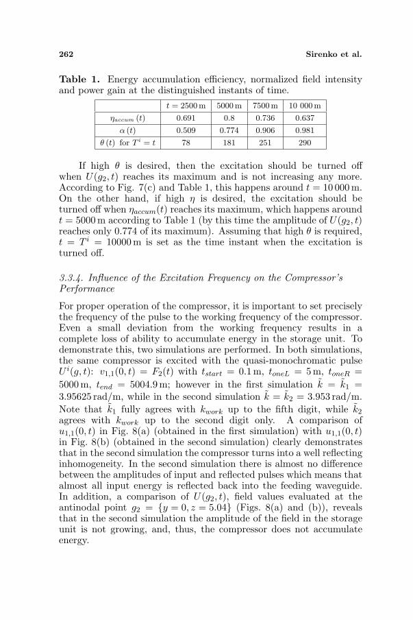
262 Sirenko et al.

Table 1. Energy accumulation efficiency, normalized field intensityand power gain at the distinguished instants of time.

t = 2500 m 5000m 7500 m 10 000m

ηaccum (t) 0.691 0.8 0.736 0.637

α (t) 0.509 0.774 0.906 0.981

θ (t) for T i = t 78 181 251 290

If high θ is desired, then the excitation should be turned offwhen U(g2, t) reaches its maximum and is not increasing any more.According to Fig. 7(c) and Table 1, this happens around t = 10 000 m.On the other hand, if high η is desired, the excitation should beturned off when ηaccum(t) reaches its maximum, which happens aroundt = 5000m according to Table 1 (by this time the amplitude of U(g2, t)reaches only 0.774 of its maximum). Assuming that high θ is required,t = T i = 10000 m is set as the time instant when the excitation isturned off.

3.3.4. Influence of the Excitation Frequency on the Compressor’sPerformance

For proper operation of the compressor, it is important to set preciselythe frequency of the pulse to the working frequency of the compressor.Even a small deviation from the working frequency results in acomplete loss of ability to accumulate energy in the storage unit. Todemonstrate this, two simulations are performed. In both simulations,the same compressor is excited with the quasi-monochromatic pulseU i(g, t): v1,1(0, t) = F2(t) with tstart = 0.1m, toneL = 5 m, toneR =5000m, tend = 5004.9 m; however in the first simulation k = k1 =3.95625 rad/m, while in the second simulation k = k2 = 3.953 rad/m.Note that k1 fully agrees with kwork up to the fifth digit, while k2

agrees with kwork up to the second digit only. A comparison ofu1,1(0, t) in Fig. 8(a) (obtained in the first simulation) with u1,1(0, t)in Fig. 8(b) (obtained in the second simulation) clearly demonstratesthat in the second simulation the compressor turns into a well reflectinginhomogeneity. In the second simulation there is almost no differencebetween the amplitudes of input and reflected pulses which means thatalmost all input energy is reflected back into the feeding waveguide.In addition, a comparison of U(g2, t), field values evaluated at theantinodal point g2 = {y = 0, z = 5.04} (Figs. 8(a) and (b)), revealsthat in the second simulation the amplitude of the field in the storageunit is not growing, and, thus, the compressor does not accumulateenergy.


0 1500 3000 4500 6000 0 1500 3000 4500 6000 [ ]t m

(a) (b)

1.0

0.0

–1.0

15

0

–15

( )1,1 0,u t ( )1,1 0,u t

( )2 ,U g t ( )2 ,U g t

Figure 8. Influence of the central frequency k of the excitationpulse on the compressor’s ability to accumulate energy: (a) Thecentral frequency coincides exactly with the working one k = kwork =3.95625 rad/m; (b) The central frequency is slightly incorrect k =3.953 rad/m.

3.3.5. Influence of the Wall Loss on the Compressor’s Performance

The design and analysis above is performed assuming that the wallsof the compressor are PEC. To make the model more realistic, andquantify the effects of this on the results, a compressor with wallsconstructed from non-perfectly conducting metal is studied. To modelthe effect of the loss, PEC walls from inside are inplaced with a 0.02mthick layer of copper (εr = 1.0, σ0 = 5.7 · 107 S/m), see Fig. 9(a). Thismore “realistic” compressor is excited with the quasi-monochromaticpulse U i(g, t): v1,1(0, t) = F2(t) with k = 3.95625 rad/m, tstart = 0.1 m,toneL = 5m, toneR = 5000 m, tend = 5004.9m. Introduction of the lossylayer does not lead to any visible difference in the processes of energyaccumulation (compare Figs. 9(b)–(e) with Fig. 6(c) or with Fig. 8(a),but note that in the cases presented in Fig. 6 the duration of excitationis shorter). The introduction of the lossy layer changes negligibly theeigenfrequency of the storage unit (because the geometrical parametersof the storage unit are affected), but the important fact is that the wallsloss does not affect essentially the energy accumulation process.

264 Sirenko et al.

( )1,1 0,v t

1.0

0.0

–1.0

0.1

0.0

–0.1

1.0

0.0

–1.0

20

0

–20

( )1,1 0,u t

( )1,2 2,u L t ( )2 ,U g t

0 2000 4000 6000 [ ]t m 0 2000 4000 6000 [ ]t m

0 2000 4000 6000 [ ]t m0 2000 4000 6000 [ ]t m

(b) (c)

(d) (e)

absorbing layer thickness is 0.02 m

1L 2L

(a)

Figure 9. Compressor with the absorbing walls excited by along quasi-monochromatic pulse: (a) Geometry of the compressor;(b)–(d) Amplitudes of the incident, reflected and transmitted pulseson the virtual boundaries L1 (z = 0) and L2 (z = L2);(e) Electric field (Ex component) intensity in the antinodal pointg2 = {y = 0, z = 5.04}.

3.4. Final Design and Discussions on Performance

Finally, setting TE0,1,12 oscillation on the frequency kwork =3.95625 rad/m as the working one, the Q-factor of the compressoris determined: Q = 7912.5 (see (13), Rek = 3.95625 and Imk =−0.00025). The duration of excitation is set as T i = 10000 m, andthe switch operates as following: until the instant of time t = 10000 mit is locked, and starting from t = 10001 m it is unlocked. On theshort time interval 10000 ≤ t ≤ 10001 the specific conductivity of the


medium inside the discharge tubes changes from σ0 = 5.7 · 104 S/mdown to σ0 = 0. The whole compressor operates as following: duringthe energy accumulation interval 0 < t < 10000m it is excited withthe long quasi-monochromatic pulse U i(g, t): v1,1(0, t) = F2(t) withk = kwork, tstart = 0.1m, toneL = 5m, toneR = 9995 m, tend = 10000 m,the excitation ends at the moment of time t = T i = 10000m, theswitch unlocks and a high-power short RF pulse is exhausted into theoutput waveguide through the virtual boundary L2 during the timeT s

2 ≈ 10025.5 − 10004 = 21.5m (Fig. 7(d)). The duration of theoutput (compressed) pulse T s

2 is a little longer than double length ofthe storage unit d2 (see Fig. 1), it is expected as the compressor withunlocked switch is not a resonant structure and all the accumulatedenergy immediately released. It should be noted here that duringthe exhaust interval 10004 < t < 10025.5m the amplitude of theinstantaneous power of the compressed pulse P s

2 (t) is 325 times and16250 times higher than the maximum amplitudes of the instantaneouspowers P i

1(t) and P s2 (t) (associated with the excitation and the pulse

seeped out into the output waveguide) during the energy accumulationinterval 0 < t < 10000m (Fig. 7).

Thus, for the compressor with the storage unit’s length of d2 =10.0m (see Fig. 1), the working frequency kwork = 3.95625 rad/m (theworking wavelength λwork ≈ 1.588m), the following characteristics areobtained: the optimal duration of excitation for the highest power gainT i = 10 000 m = 33.3564µs, the duration of compressed output pulseT s

2 = 21.5m = 71.7163 ns, the degree of compression β = T i/T s2 ≈ 465,

the efficiency η = W s2 ( 10004; 10025.5)/W i

1(0; T i) ≈ 0.6238, the powergain θ = β ·η ≈ 290. The compressor’s efficiency η is a bit smaller thanthe efficiency of energy accumulation ηaccum(T i) because a fraction ofthe accumulated energy is distributed among the short intensive spikein the reflected signal and the tail following the main output pulse.It should be noted here that due to the scalability of the Maxwell’sequations, it is straightforward to transfer the results obtained usingthe scheme presented in this paper to any other geometrically similarstructure. If the frequency is increased by a certain factor, then the(spatial) dimensions of the geometries and the time t (as it is measuredin meters) should be divided by that factor to obtain the same results.

It should be emphasized here that the rigorous real-time studyof the energy accumulation and exhaust processes allows preciseadjustment of the critical parameters of a compressor (such asgeometry of a coupling window (see Section 3.3.2), excitation frequency(see Section 3.3.4) and duration of excitation (see Section 3.3.3)) toobtain maximum efficiency or power gain. This is one of the advantagesof the presented time-domain rigorous modeling-based approach, as

266 Sirenko et al.

parameters of a model could be changed on the fly and effects of thesechanges could be obtained with high accuracy. Such optimizationmight be hard to achieve using simplified theories or experimental-based approach.

Having said that, the final characteristics given above may seemoveroptimistic, when compared to experimental findings presentedin [2, 10–12, 14] for similar types of compressors. This difference canmainly be attributed to the difference between the excitation durations;a relatively long duration of excitation is used in this paper, whichnaturally results in rather high values of the degree of compressionand the power gain for high-Q cavities. It should be noted here thatthis duration is found to be optimal to obtain the highest power gain;in the experimental results, such long duration might have not beenemployed due to practical limitations of the generators. If the durationof excitation in the example presented above is reduced, it can beobserved that the characteristics will get closer to the ones obtainedexperimentally.

4. BRIEF DESCRIPTION OF THE NUMERICALTECHNIQUE

It can be concluded without hesitation that this paper demonstratesthe advantages of the time-domain analysis over its frequency-domain(steady-state) counterpart for the design of microwave compressors.In this work, because of this reason, FDTD method is used forcharacterizing transient energy accumulation in compressors.

To enable the use of FDTD methods for solving the open initial-boundary value problem, which mathematically models the waveinteractions on compressors (Section 2.1), the computation domainhas to be truncated. Traditional methods involving perfectly matchedlayers and approximate absorbing boundary conditions [37] cannot beused in this work because of the enormous length of the simulationtimes needed to observe weakly-decaying highly-oscillatory fields (thenumber of time steps can easily exceed 1000000); these methods willsimply introduce numerical error build up for such long simulationtimes. To ensure the reliability of the final results at the end of longtime marching, exact absorbing conditions (EACs) proposed in [19–21] are utilized here. These conditions are derived using rigorousmathematical manipulations and consequently are mathematicallyexact. Papers [19, 20] focus on the derivation EACs for axiallysymmetric and 2-D plane-parallel waveguide problems, respectively.Paper [19] also describes a blocked FFT-based scheme for reducing thecomputational cost of the temporal convolutions present in non-local


EACs to O(T log2 T ) from O(T 2). It should be noted here that thisacceleration scheme is numerically exact.

These two advanced techniques, namely EACs and the blockedFFT-acceleration scheme, when combined with FDTD method, enablethe accurate and efficient analysis of weakly-decaying highly-oscillatorytransients on compressors. In addition, real-time observationcapability that comes with any time domain method renders theFDTD method with FFT-accelerated EACs a preferred design toolfor engineers.

5. CONCLUSION

It is impossible to design a microwave energy compressor without in-depth understanding of the non-monotonic physical behavior of thehighly resonant high power pulses present in the storage unit. Thiscan successfully be achieved by a design scheme that heavily dependson time-domain analysis. In this work, practically for the first time, allphysical processes inside a microwave energy compressor are studied intime-domain in detail from the very beginning of the excitation rightuntil the end of the accumulated energy’s exhaust. Additionally, effectsof compressor’s design and excitation parameters on performance ofcompressor are quantified.

The methodology and the results presented here are valuable indesign and fabrication of microwave compressors. In Part II of thispaper, the methodology developed here will be used to design a novelcombined compressor/radiator antenna element for a phased array.

REFERENCES

1. Bossart, R., P. Brown, J. Mourier, I. V. Syratchev, and L. Tanner,“High-power microwave pulse compression of klystrons by phase-modulation if high-Q storage cavities,” CERN CLIC-Notes,No. 592, 2004.

2. Vikharev, A. L., O. A. Ivanov, A. M. Gorbachev, S. V. Kuzikov,V. A. Isaev, V. A. Koldanov, M. A. Lobaev, J. L. Hirshfield,M. A. LaPointe, O. A. Nezhevenko, S. H. Gold, and A. K. Kinkead,“Active compression of RF pulses,” Quasi-optical Control ofIntense Microwave Transmission, J. L. Hirshfield and M. I. Petelin(eds.), 199–218, Springer, Netherlands, 2005.

3. Yushkov, Y. G., N. N. Badulin, A. P. Batsula, A. I. Mel’nikov,S. A. Novikov, S. V. Razin, and E. L. Shoshin, “A nanosecondpulse-compression microwave radar,” Telecommunications andRadio Engineering, Vol. 54, No. 2, 92–98, 2000.

268 Sirenko et al.

4. Schamiloglu, E., “High power microwave sources and applica-tions,” 2004 IEEE MTT-S Digest, 1001–1004, 2004.

5. Benford, J., “Space applications of high-power microwaves,” IEEETrans. Plasma Sci., Vol. 36, No. 3, 569–581, 2008.

6. Gaponov-Grekhov, A. V. and V. L. Granatstein, Applications ofHigh-power Microwaves, Artech House, Boston, 1994.

7. Bluhm, H., Pulsed Power Systems. Principles and Applications,Springer, Berlin, 2006.

8. Andreev, A. D., E. G. Farr, and E. Schamiloglu, “Asimplified theory of microwave pulse compression,” Circuit andElectromagnetic System Design Notes, No. 57, 2008.

9. Baum, C. E., “Options in microwave pulse compression,” Circuitand Electromagnetic System Design Notes, No. 68, 2010.

10. Vikharev, A. L., A. M. Gorbachev, O. A. Ivanov, V. A. Isaev,S. V. Kuzikov, B. Z. Movshevich, J. L. Hirshfield, and S. H. Gold,“Active Bragg compressor of 3-cm wavelength microwave pulses,”Radiophys. Quantum Electron., Vol. 51, No. 7, 539–555, 2008.

11. Artemenko, S. N., V. A. Avgustinovich, V. L. Kaminskii,P. Y. Chumerin, and Y. G. Yushkov, “Experimental investigationof a 25-MW microwave (3-cm range) compressor prototype,”Technical Physics, Vol. 45, No. 12, 1608–1611, 2000.

12. Tantawi, S. G., R. D. Ruth, A. E. Vlieks, and M. Zolotorev,“Active high-power RF pulse compression using optically switchedresonant delay lines,” IEEE Trans. Microw. Theory Tech., Vol. 45,No. 8, 1486–1492, 1997.

13. Vikharev, A. L., A. M. Gorbachev, O. A. Ivanov, V. A. Isaev,S. V. Kuzikov, A. L. Kolysko, and M. I. Petelin, “Active microwavepulse compressor utilizing an axisymmetric mode of a circularwaveguide,” Technical Physics Letters, Vol. 24, No. 10, 791–792,1998.

14. Farr, E. G., L. H. Bowen, W. D. Prather, and C. E. Baum,“Microwave pulse compression experiments at low and highpower,” Circuit and Electromagnetic System Design Notes, No. 63,2010.

15. Tamura, F. and S. G. Tantawi, “Development of high powerX-band semiconductor microwave switch for pulse compressionsystems of future linear colliders,” Phys. Rev. Spec. Top. Accel.Beams, Vol. 5, 062001, 2002.

16. Ivanov, O. A., A. A. Vikharev, A. M. Gorbachev, V. A. Isaev,M. A. Lobaev, A. L. Vikharev, S. V. Kuzikov, J. L. Hirshfield, andM. A. LaPointe, “Active quasioptical Ka-band rf pulse compressor


switched by a diffraction grating,” Phys. Rev. Spec. Top. Accel.Beams, Vol. 12, 093501, 2009.

17. Kuzmitchev, I. K., P. M. Melezhyk, V. L. Pazynin, K. Y. Sirenko,Y. K. Sirenko, O. S. Shafalyuk, and L. G. Velychko, “Modelsynthesis of energy compressors,” Radiophysics and Electronics:Sci. Works Collection, Vol. 13, No. 2, 166–172, 2008.

18. Chernobrovkin, R. E., I. V. Ivanchenko, A. M. Korolev,N. A. Popenko, and K. Y. Sirenko, “The novel microwave stop-band filter,” Active and Passive Electronic Components, Vol. 2008,2008.

19. Sirenko, K., V. Pazynin, Y. Sirenko, and H. Bagci, “An FFT-accelerated FDTD scheme with exact absorbing conditions forcharacterizing axially symmetric resonant structures,” Progress InElectromagnetics Research, Vol. 111, 331–364, 2011.

20. Sirenko, K. Y. and Y. K. Sirenko, “Exact absorbing conditionsin the initial boundary-value problems of the theory of openwaveguide resonators,” Comput. Math. Math. Phys., Vol. 45,No. 3, 490–506, 2005.

21. Sirenko, Y. K., S. Strom, and N. P. Yashina, Modeling andAnalysis of Transient Processes in Open Resonant Structures. NewMethods and Techniques, Springer, Berlin, 2007.

22. Hairer, E., C. H. Lubich, and M. Schlichte, “Fast numericalsolution of nonlinear Volterra convolution equations,” SIAM J.Sci. Stat. Comput., Vol. 6, No. 3, 532–541, 1985.

23. Yilmaz, A. E., D. S. Weile, B. Shanker, J.-M. Jin, andE. Michielssen, “Fast analysis of transient scattering in lossymedia,” IEEE Antennas Wireless Propagat. Lett., Vol. 1, No. 1,14–17, 2002.

24. Bagci, H., A. E. Yilmaz, and E. Michielssen, “A fast hybridTDIE-FDTD-MNA scheme for analyzing cable-induced transientcoupling into shielding enclosures,” Proc. IEEE Int. Symp.Electromagn. Compat., Vol. 3, 828–833, 2005.

25. Bagci, H., A. E. Yilmaz, V. Lomakin, and E. Michielssen, “Fastsolution of mixed-potential time-domain integral equations forhalf-space environments,” IEEE Trans. Geosci. Remote Sensing,Vol. 43, No. 2, 269–279, 2005.

26. Bagci, H., A. E. Yilmaz, and E. Michielssen, “FFT-acceleratedMOT-based solution of time-domain BLT equations,” Proc. IEEEInt. Antennas Propagat. Symp., 1175–1178, 2006.

27. Bagci, H., A. E. Yilmaz, J.-M. Jin, and E. Michielssen, “Fast andrigorous analysis of EMC/EMI phenomena on electrically large

270 Sirenko et al.

and complex structures loaded with coaxial cables,” IEEE Trans.Electromagn. Compat., Vol. 49, No. 2, 361–381, 2007.

28. Bagci, H., A. E. Yilmaz, and E. Michielssen, “An FFT-acceleratedtime-domain multiconductor transmission line simulator,” IEEETrans. Electromagn. Compat., Vol. 52, No. 1, 199–214, 2010.

29. Sirenko, Y. K., L. G. Velychko, and F. Erden, “Time-domain and frequency-domain methods combined in the studyof open resonance structures of complex geometry,” Progress InElectromagnetics Research, Vol. 44, 57–79, 2004.

30. Velychko, L. G., Y. K. Sirenko, and O. S. Shafalyuk, “Time-domain analysis of open resonators. Analytical grounds,” ProgressIn Electromagnetics Research, Vol. 61, 1–26, 2006.

31. Velychko, L. G. and Y. K. Sirenko, “Controlled changes in spectraof open quasi-optical resonators,” Progress In ElectromagneticsResearch B, Vol. 16, 85–105, 2009.

32. Karmel, P. R, G. D. Colef, and R. L. Camisa, Introduction toElectromagnetic and Microwave Engineering, John Wiley, NewYork, 1998.

33. Shestopalov, V. P., A. A. Kirilenko, and L. A. Rud’, ResonanceWave Scattering. Vol. 2. Waveguide Discontinuities, NaukovaDumka, Kiev, 1986 (in Russian).

34. Pozar, D. M., Microwave Engineering, Wiley, New York, 1998.35. Belous, O. I., A. A. Kirilenko, V. I. Tkachenko, A. I. Fisun, and

A. M. Fursov, “Excitation of an open stripline resonator by aplane waveguide,” Radiophys. Quantum Electron., Vol. 37, No. 3,181–189, 1994.

36. Sirenko, Y. K. and S. Strom, Modern Theory of Gratings.Resonant Scattering: Analysis Techniques and Phenomena,Springer, Berlin, 2010.

37. Taflove, A. and S. C. Hagness, Computational Electrodynamics:The Finite-difference Time-domain Method, Artech House,Boston, 2005.

Documents

COMPRESSION AND RADIATION OF HIGH-POWER SHORT RF PULSES. I. ENERGY